Optimal design of work-in-process buffers

ARTICLE IN PRESS

0925-5273/$ - se

doi:10.1016/j.ijp

�Correspondi

rials, Departme

gineering, Univ

465 Porto, Port

fax: +351 22 50

E-mail addre

(M. Matos), en

Int. J. Production Economics 99 (2006) 144–155

www.elsevier.com/locate/ijpe

Optimal design of work-in-process buffers

Jose Fariaa,�, Manuel Matosa,b, Eusebio Nunesc

aDepartment of Electrical and Computers Engineering, FEUP—Faculty of Engineering, University of Porto,

Rua Roberto Frias s/n, 4200-465 Porto, PortugalbINESC Porto, Rua Roberto Frias, 4200-465 Porto, Portugal

cSchool of Engineering, University of Minho, Campus de Gualtar, 4710-057 Braga, Portugal

Available online 5 February 2005

Abstract

When customers demand for very short lead-times and for a strict respect of the delivery schedules, it becomes

difficult to avoid the existence of relatively large work-in-process buffers. As the buffers will also increase dramatically

the production costs, their design (location and capacity) should be carefully analyzed and optimized, a task that

becomes rather complex for large production systems. This paper firstly introduces a series of fundamental concepts

related to the reliability of production systems. Then, the rationale of an analysis method oriented to this class of

systems will be presented, together with its two main components, the modelling framework and the evaluation

algorithm. The method allows analysing several issues of the design and operation of the production systems, namely

the redundancy of equipment, the layout of the cells and the maintenance policies. To illustrate its practical usefulness

and enlighten the kind of results that the method can provide, a numerical example concerning the design of work-in-

process buffers of a just-in-time manufacturing system will be presented in the final part of the paper.

r 2005 Elsevier B.V. All rights reserved.

Keywords: Production systems; Reliability; Modelling; Evaluation; Economical analysis

1. Introduction

Nowadays, in order to remain competitive,manufacturing companies have to offer their

e front matter r 2005 Elsevier B.V. All rights reserve

e.2004.12.019

ng author. Laboratory of Catalysis and Mate-

nt of Chemical Engineering, Faculty of En-

ersity of Porto, Rua Roberto Frias s/n, 4200-

gal. Tel.: +351 22 508 1831;

8 1443.

sses: [email protected] (J. Faria), [email protected]

[email protected] (E. Nunes).

clients high-quality products at low cost and shortlead times (very short, in fact). These demandingrequirements are driving manufacturing compa-nies to increase their cooperation within value-added networks, where participants are tied byjust-in-time (jit) deliveries and where the failure ofa single manufacturing unit may have a dramaticconsequence on the overall performance of thenetwork. In spite of the worldwide intensive effortsmade during the last two decades in order toreduce working inventory levels through the

d.

www.elsevier.com/locate/dsw

ARTICLE IN PRESS

J. Faria et al. / Int. J. Production Economics 99 (2006) 144–155 145

adoption of jit techniques, there are situationssuch that the existence of relatively largework-in-process (wip) buffers can not be avoided,as they are the only way to guarantee the strictdeliver schedules required by the networkedoperation. Buffers filter the unbalance of manu-facturing cells having different production ratesand prevent the propagation of the disturbancesfrom the faulty manufacturing cells to the down-stream cells. However, they have a major draw-back—the dramatic increase of the operationalcost—so that their design should come from aneconomical analysis (Mahadevan and Narendran,1993) that balances the implementation cost(stored materials and occupied area) with the levelof service provided to the consumers (Berg et al.,1994) and the productivity improvement achievedby the fact that the overall production flowbecomes less sensitive to the failures of theindividual equipments.

This paper presents a reliability analysis methodthat will help managers in the design of the work-in-process buffers. Existing methods and tools forthe analysis and performance evaluation of pro-duction systems often impose severe restrictions onthe structure and behaviour of the systems thatlimit its application to relatively simple systems.For example Giordano (2002) considers theoptimization of the safety stock for a single-parttype, single unreliable machine production system,Van Ryzin et al. (1993) investigates optimalproduction control for a tandem of two machines,and Moinzadeh (1997) analyses an unreliablebottleneck assuming constant production anddemand rate, constant restoration time andexponential failure processes. In comparison, themethod that will be presented here considerablyrelax the basic assumptions and extends theapplication scope. Some of its main features arethe ability to deal with processes having arbitrarydistributions (and not only exponential distribu-tions as it often happens in reliability tools), theuse of a hierarchical modelling framework, thatallows representing the overall structure of thesystem and the internal behaviour of each manu-facturing unit at different modelling levels; the useof a standard canonical model to represent thebehaviour of each production subsystem; and the

evaluation of the overall reliability indices from aglobal system model obtained from the aggrega-tion of the subsystems’ canonical models.

After this introduction, a structural and beha-vioural analysis of the production systems will bepresented in Section 2, in order to introduce a setof concepts related to the reliability of thesesystems that will clarify the rationale and therequirements of the method. Sections 3 and 4 willdiscuss the two components of the method: Themodelling framework and the evaluation algo-rithm. The practical application of the methodwill be illustrated in Section 5, through anumerical example concerning the design of thebuffers of a just-in-time manufacturing system.Finally, Section 6 discusses current limitations ofthe method and some extensions that are beingdeveloped.

2. Production systems analysis

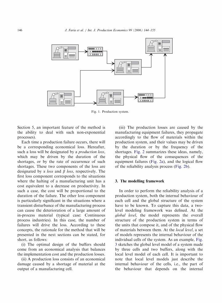
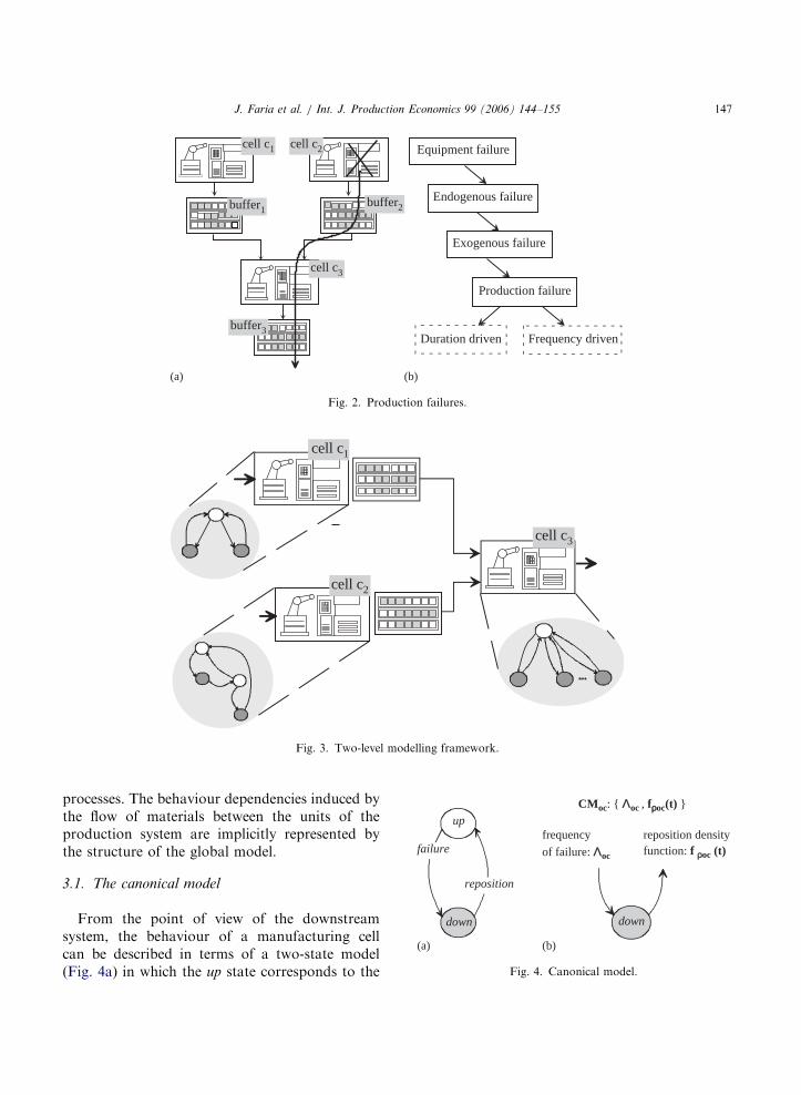
A production system is seen as a networkarrangement of cells that interact according to aproducer/consumer scheme. As shown in Fig. 1,the output of a manufacturing cell may be linkeddirectly to the input of one or more downstreamcells but, also, it may exist an intermediate bufferbetween the cells, containing wip material. Aproduction failure will occur when the normal flowof materials within the production system isdisturbed and a materials shortage occurs. Ashortage at the output of a cell may occur becausethat cell has halted its operation due to anendogenous failure, i.e., a failure of one of itsinternal equipments, or to an exogenous failure,i.e., a failure of a external equipment that hascaused a material shortage at the input of the cell.When a production failure occurs at a cell, itwill not be propagated immediately to the down-stream cells if there is a buffer at the output of thefailed cell. In such case, there will be a propagation

delay before the downstream cells ‘‘see’’ thematerials shortage. Typically, this will be a non-exponential random delay that depends on thequantity of material existing in the buffer when theshortage has occurred (as it will be discussedwithin the context of the numerical example of

ARTICLE IN PRESS

Fig. 1. Production system.

J. Faria et al. / Int. J. Production Economics 99 (2006) 144–155146

Section 5, an important feature of the method isthe ability to deal with such non-exponentialprocesses).

Each time a production failure occurs, there willbe a corresponding economical loss. Hereafter,such a loss will be designated by a production loss,which may be driven by the duration of theshortages, or by the rate of occurrence of suchshortages. These two components of the loss aredesignated by a loss and b loss, respectively. Thefirst loss component corresponds to the situationswhere the halting of a manufacturing unit has acost equivalent to a decrease on productivity. Insuch a case, the cost will be proportional to theduration of the failure. The other loss componentis particularly significant in the situations where atransient disturbance of the manufacturing processcan cause the deterioration of a large amount ofin-process material (typical case: Continuousprocess industries). In this case, the number offailures will drive the loss. According to theseconcepts, the rationale for the method that will bepresented in the next sections can be stated, forshort, as follows:

(i) The optimal design of the buffers shouldcome from an economical analysis that balancesthe implementation cost and the production losses.

(ii) A production loss consists of an economicaldamage caused by a shortage of material at theoutput of a manufacturing cell.

(iii) The production losses are caused by themanufacturing equipment failures, they propagateaccordingly to the flow of materials within theproduction system, and their values may be drivenby the duration or by the frequency of theshortages. Fig. 2 summarizes these ideas, namely,the physical flow of the consequences of theequipment failures (Fig. 2a), and the logical flowof the reliability analysis process (Fig. 2b).

3. The modelling framework

In order to perform the reliability analysis of aproduction system, both the internal behaviour ofeach cell and the global structure of the systemhave to be known. To capture this data, a two-level modeling framework was defined. At theglobal level, the model represents the overallstructure of the production system in terms ofthe units that compose it, and of the physical flowof materials between them. At the local level, a setof models represents the internal behaviour of theindividual cells of the system. As an example, Fig.3 sketches the global level model of a system madeby three cells and two buffers, along with thelocal level model of each cell. It is important tonote that local level models just describe theinternal behaviour of the cells, i.e., the part ofthe behaviour that depends on the internal

ARTICLE IN PRESS

Endogenous failure

Exogenous failure

Production failure

Duration driven Frequency driven

(a) (b)

buffer1

Equipment failurecell c1 cell c2

cell c3

buffer2

buffer3

Fig. 2. Production failures.

cell c2

cell c3

cell c1

Fig. 3. Two-level modelling framework.

up

downdown

(a) (b)

reposition

failurefrequency

of failure: ΛΛoc

reposition densityfunction: f ρoc (t)

CMoc: { Λoc , fρoc(t) }

Fig. 4. Canonical model.


processes. The behaviour dependencies induced bythe flow of materials between the units of theproduction system are implicitly represented bythe structure of the global model.

3.1. The canonical model

From the point of view of the downstreamsystem, the behaviour of a manufacturing cellcan be described in terms of a two-state model(Fig. 4a) in which the up state corresponds to the

ARTICLE IN PRESS


situations where the cell produces its outputaccordingly to the schedule, and the down state,represents the situations where the cell is haltedand the normal flow of materials is interrupted.For the failure processes, normally, it is reasonableto assume that the time between failures isexponentially distributed, but the same can notbe said for the reposition processes. Often, theseprocesses are deterministic or quasi-deterministic,so that their probability density functions are closeto the Dirac or to the step function, as it will beseen in Section 5. Therefore, the behaviour of anupstream cell c will be fully characterized by thecouplet fLoc; f rocðtÞg where Loc is the rate of thefailure and fro(t) is the probability density functionof the reposition process (Fig. 4b). Hereafter, thiscouplet will be designated as the output canonical

model of the cell c, and it will be denoted by Moc.As pointed out before, the output unavailability of

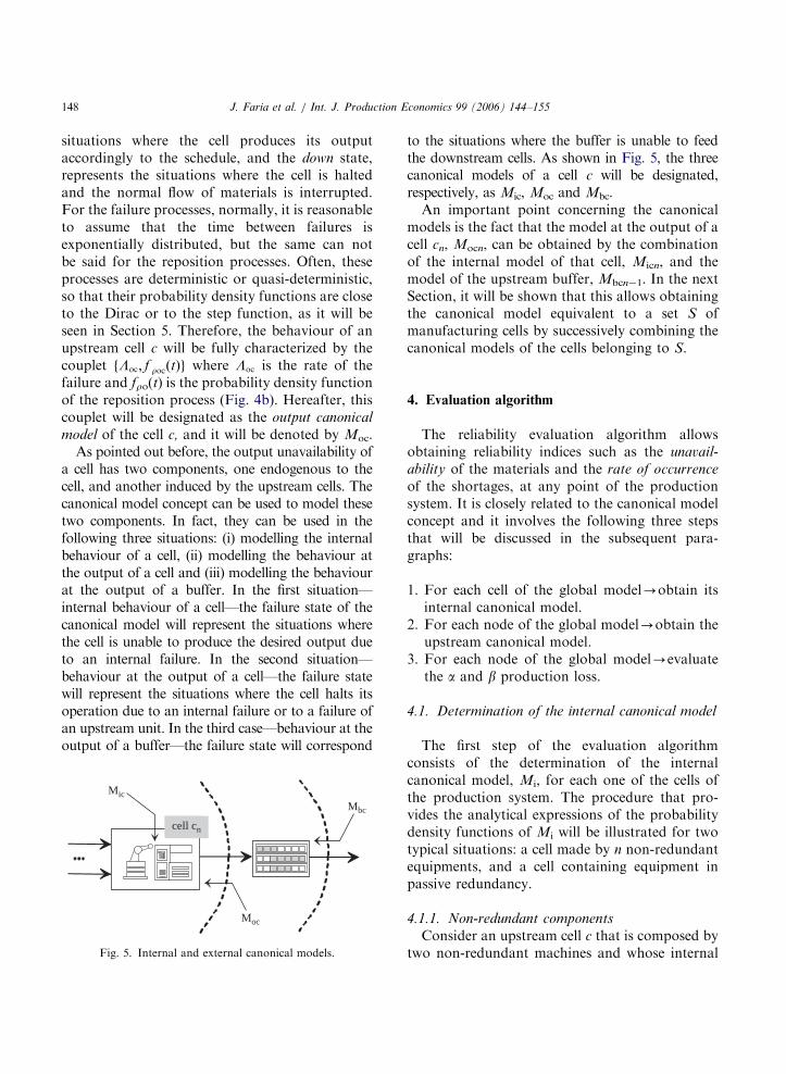
a cell has two components, one endogenous to thecell, and another induced by the upstream cells. Thecanonical model concept can be used to model thesetwo components. In fact, they can be used in thefollowing three situations: (i) modelling the internalbehaviour of a cell, (ii) modelling the behaviour atthe output of a cell and (iii) modelling the behaviourat the output of a buffer. In the first situation—internal behaviour of a cell—the failure state of thecanonical model will represent the situations wherethe cell is unable to produce the desired output dueto an internal failure. In the second situation—behaviour at the output of a cell—the failure statewill represent the situations where the cell halts itsoperation due to an internal failure or to a failure ofan upstream unit. In the third case—behaviour at theoutput of a buffer—the failure state will correspond

Mic

Moc

Mbc

cell cn

Fig. 5. Internal and external canonical models.

to the situations where the buffer is unable to feedthe downstream cells. As shown in Fig. 5, the threecanonical models of a cell c will be designated,respectively, as Mic, Moc and Mbc.

An important point concerning the canonicalmodels is the fact that the model at the output of acell cn, Mocn, can be obtained by the combinationof the internal model of that cell, Micn, and themodel of the upstream buffer, Mbcn�1. In the nextSection, it will be shown that this allows obtainingthe canonical model equivalent to a set S ofmanufacturing cells by successively combining thecanonical models of the cells belonging to S.

4. Evaluation algorithm

The reliability evaluation algorithm allowsobtaining reliability indices such as the unavail-

ability of the materials and the rate of occurrence

of the shortages, at any point of the productionsystem. It is closely related to the canonical modelconcept and it involves the following three stepsthat will be discussed in the subsequent para-graphs:

1.
For each cell of the global model-obtain itsinternal canonical model.
2.
For each node of the global model-obtain theupstream canonical model.
3.
For each node of the global model-evaluatethe a and b production loss.
4.1. Determination of the internal canonical model

The first step of the evaluation algorithmconsists of the determination of the internalcanonical model, Mi, for each one of the cells ofthe production system. The procedure that pro-vides the analytical expressions of the probabilitydensity functions of Mi will be illustrated for twotypical situations: a cell made by n non-redundantequipments, and a cell containing equipment inpassive redundancy.

4.1.1. Non-redundant components

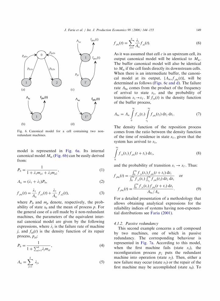
Consider an upstream cell c that is composed bytwo non-redundant machines and whose internal

ARTICLE IN PRESS

p 1n

(a)

1 1'

1

2

0

(b)

(c)

(d)

1µ

p 2nµ

p 1nλ

p cγ

p 2nλ

fρρic(t)

fρoc(t)

fρbc(t)

fρoc(t)

Λic Λoc

Λoc

1"

Fig. 6. Canonical model for a cell containing two non-

redundant machines.


model is represented in Fig. 6a. Its internalcanonical model Mic (Fig. 6b) can be easily derivedfrom:

P0 ¼1

1 þ l1mm1 þ l2mm2

; (1)

Lic ¼ ðl1 þ l2ÞP0; (2)

f ricðtÞ ¼l1

Lic

f m1ðtÞ þl2

Lic

f m2ðtÞ; (3)

where P0 and mp denote, respectively, the prob-ability of state s0 and the mean of process p. Forthe general case of a cell made by k non-redundantmachines, the parameters of the equivalent inter-nal canonical model are given by the followingexpressions, where lj is the failure rate of machinej, and fmj(t) is the density function of its repairprocess, pmj:

P0 ¼1

1 þPk

j¼1ljmmj

; (4)

Lic ¼Xk

j¼1

lj ; (5)

f ricðtÞ ¼Xk

j¼1

lj

Lic

f mjðtÞ: (6)

As it was assumed that cell c is an upstream cell, itsoutput canonical model will be identical to Mic.The buffer canonical model will also be identicalto Mic if the cell feeds directly its downstream cells.When there is an intermediate buffer, the canoni-cal model at its output, fLbc; f rbcðtÞg; will bedetermined as follows (Figs. 6c and d). The failurerate Lbc comes from the product of the frequencyof arrival to state s1, and the probability oftransition s1-s10. If fgc(t) is the density functionof the buffer process,

Lbc ¼ Lic

Z1

0

f gcðt1Þ

Z1

t1

f ricðt2Þ dt2 dt1: (7)

The density function of the reposition processcomes from the ratio between the density functionof the time of residence in state s10, given that thesystem has arrived to s1,

Z1

0

f gcðt1Þ f ricðt þ t1Þ dt1; (8)

and the probability of transition s1 ! s10 : Thus:

f rbcðtÞ ¼

R1

0f gcðt1Þ f ricðt þ t1Þ dt1R1

0f gcðt1Þ

R1

t1f ricðt2Þ dt2 dt1

or

f rbcðtÞ ¼

R1

0f gcðt1Þ f ricðt þ t1Þ dt1

Lbc=Lic

: ð9Þ

For a detailed presentation of a methodology thatallows obtaining analytical expressions for thereliability indices of systems having non-exponen-tial distributions see Faria (2001).

4.1.2. Passive redundancy

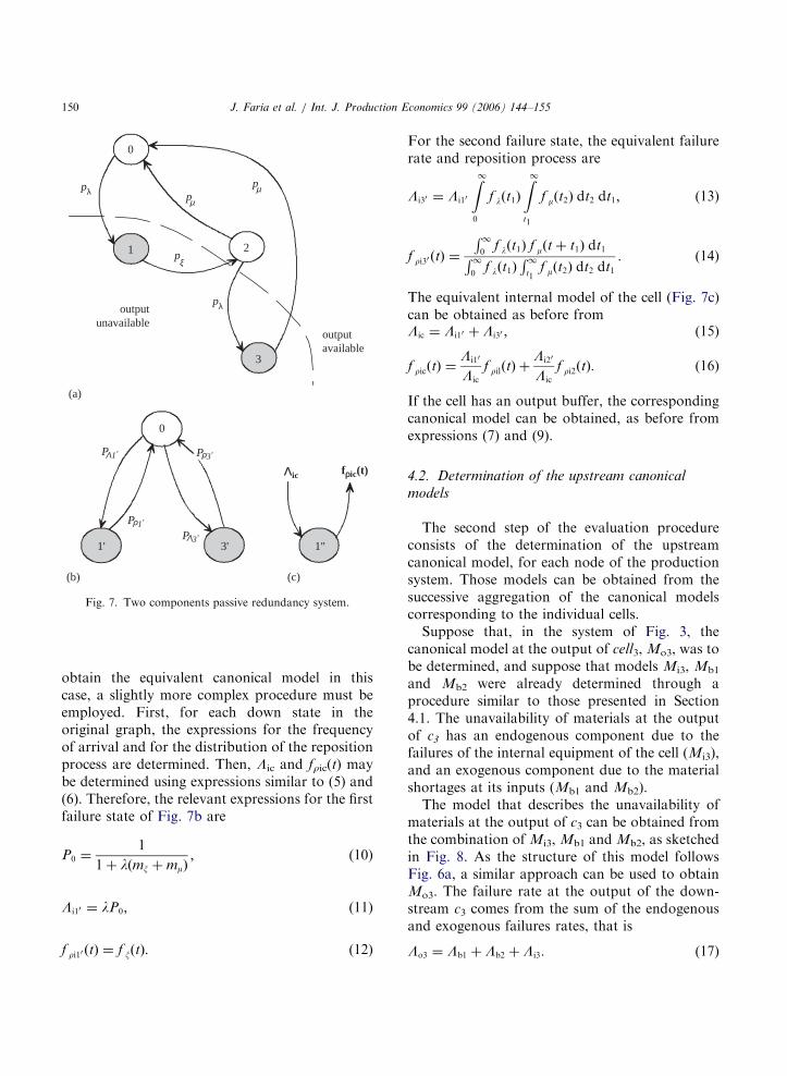
This second example concerns a cell composedby two machines, one of which in passiveredundancy. The corresponding behaviour isrepresented in Fig. 7a. According to this model,when the first machine fails (state s1), thereconfiguration process px puts the redundantmachine into operation (state s2). Then, either anew failure may occur (state s3) or the repair of thefirst machine may be accomplished (state s0). To

ARTICLE IN PRESS

pλ

pλ

0

3

21

(a)

3'

0

1'

(b) (c)

1"

outputavailable

outputunavailable

pµ

pµ

pξ

fρic(t)

P 1'

Λic

ρP 3'Λ

P 1'Λ P 3'ρ

Fig. 7. Two components passive redundancy system.


obtain the equivalent canonical model in thiscase, a slightly more complex procedure must beemployed. First, for each down state in theoriginal graph, the expressions for the frequencyof arrival and for the distribution of the repositionprocess are determined. Then, Lic and fric(t) maybe determined using expressions similar to (5) and(6). Therefore, the relevant expressions for the firstfailure state of Fig. 7b are

P0 ¼1

1 þ lðmx þ mmÞ; (10)

Li10 ¼ lP0; (11)

f ri10 ðtÞ ¼ f xðtÞ: (12)

For the second failure state, the equivalent failurerate and reposition process are

Li30 ¼ Li10

Z1

0

f lðt1Þ

Z1

t1

f mðt2Þ dt2 dt1; (13)

f ri30 ðtÞ ¼

R1

0f lðt1Þ f mðt þ t1Þ dt1R1

0f lðt1Þ

R1

t1f mðt2Þ dt2 dt1

: (14)

The equivalent internal model of the cell (Fig. 7c)can be obtained as before fromLic ¼ Li10 þ Li30 ; (15)

f ricðtÞ ¼Li10

Lic

f rilðtÞ þLi20

Lic

f ri2ðtÞ: (16)

If the cell has an output buffer, the correspondingcanonical model can be obtained, as before fromexpressions (7) and (9).

4.2. Determination of the upstream canonical

models

The second step of the evaluation procedureconsists of the determination of the upstreamcanonical model, for each node of the productionsystem. Those models can be obtained from thesuccessive aggregation of the canonical modelscorresponding to the individual cells.

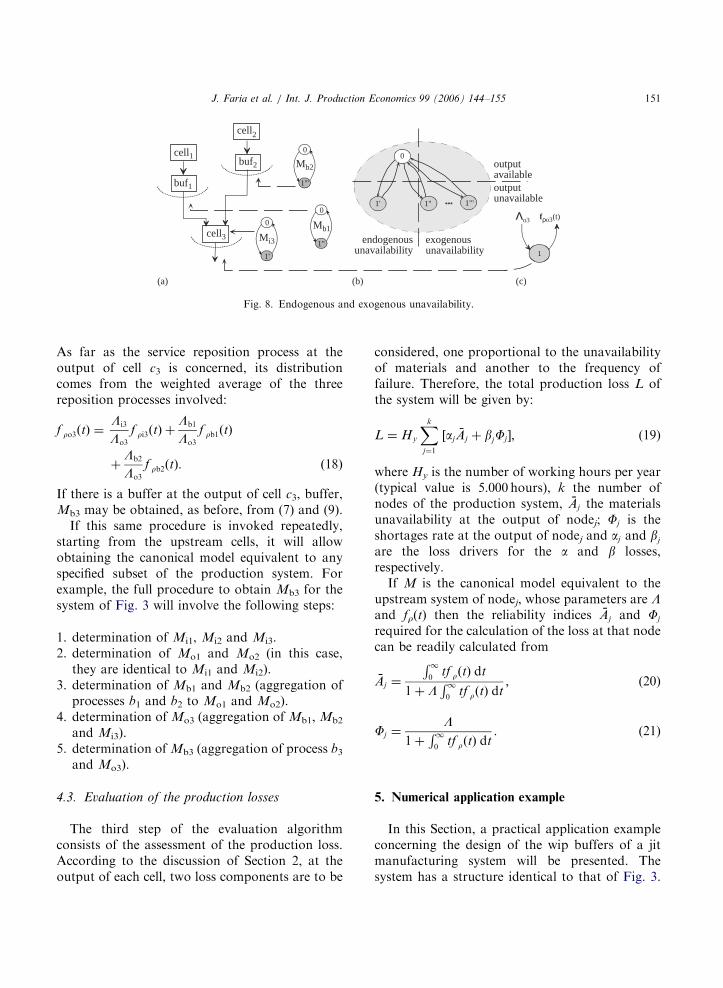
Suppose that, in the system of Fig. 3, thecanonical model at the output of cell3, Mo3, was tobe determined, and suppose that models Mi3, Mb1

and Mb2 were already determined through aprocedure similar to those presented in Section4.1. The unavailability of materials at the outputof c3 has an endogenous component due to thefailures of the internal equipment of the cell (Mi3),and an exogenous component due to the materialshortages at its inputs (Mb1 and Mb2).

The model that describes the unavailability ofmaterials at the output of c3 can be obtained fromthe combination of Mi3, Mb1 and Mb2, as sketchedin Fig. 8. As the structure of this model followsFig. 6a, a similar approach can be used to obtainMo3. The failure rate at the output of the down-stream c3 comes from the sum of the endogenousand exogenous failures rates, that is

Lo3 ¼ Lb1 þ Lb2 þ Li3: (17)

ARTICLE IN PRESS

0

1'''

1"'1' 1"

0

buf1

Mb2

Mb10

1'

Mi3

cell2

cell1

0

1"

(c)

1

(b)(a)

outputunavailable

outputavailable

endogenousunavailability

exogenousunavailability

fρo3(t)Λo3

buf2

cell3

Fig. 8. Endogenous and exogenous unavailability.


As far as the service reposition process at theoutput of cell c3 is concerned, its distributioncomes from the weighted average of the threereposition processes involved:

f ro3ðtÞ ¼Li3

Lo3

f ri3ðtÞ þLb1

Lo3

f rb1ðtÞ

þLb2

Lo3

f rb2ðtÞ: ð18Þ

If there is a buffer at the output of cell c3, buffer,Mb3 may be obtained, as before, from (7) and (9).

If this same procedure is invoked repeatedly,starting from the upstream cells, it will allowobtaining the canonical model equivalent to anyspecified subset of the production system. Forexample, the full procedure to obtain Mb3 for thesystem of Fig. 3 will involve the following steps:

1.
determination of Mi1, Mi2 and Mi3. 2. determination of Mo1 and Mo2 (in this case,
they are identical to Mi1 and Mi2).
3. determination of Mb1 and Mb2 (aggregation of
processes b1 and b2 to Mo1 and Mo2).
4. determination of Mo3 (aggregation of Mb1, Mb2
and Mi3).
5. determination of Mb3 (aggregation of process b3
and Mo3).

4.3. Evaluation of the production losses

The third step of the evaluation algorithmconsists of the assessment of the production loss.According to the discussion of Section 2, at theoutput of each cell, two loss components are to be

considered, one proportional to the unavailabilityof materials and another to the frequency offailure. Therefore, the total production loss L ofthe system will be given by:

L ¼ Hy

Xk

j¼1

½ajAj þ bjFj�; (19)

where Hy is the number of working hours per year(typical value is 5.000 hours), k the number ofnodes of the production system, Aj the materialsunavailability at the output of nodej; Fj is theshortages rate at the output of nodej and aj and bj

are the loss drivers for the a and b losses,respectively.

If M is the canonical model equivalent to theupstream system of nodej, whose parameters are Land fr(t) then the reliability indices Aj and Fj

required for the calculation of the loss at that nodecan be readily calculated from

Aj ¼

R1

0tf rðtÞ dt

1 þ LR1

0tf rðtÞ dt

; (20)

Fj ¼L

1 þR1

0tf rðtÞ dt

: (21)

5. Numerical application example

In this Section, a practical application exampleconcerning the design of the wip buffers of a jitmanufacturing system will be presented. Thesystem has a structure identical to that of Fig. 3.

ARTICLE IN PRESS

(b)

(a)

t t

t t

t t

I

(c)

I

I

fb(t)

fb(t)

fb(t)

∆

∆

∆

∆

Fig. 9. Types of probability density functions.


It contains two manufacturing cells (cell c1 and cellc2) that feed an assembly cell (cell c3) operating jit,which means that the finished parts produced at itsoutput are delivered directly to the clients withoutany temporary storage. Cell c1 is made by twoidentical non-redundant machines, whereas cell c2

is made by two machines in passive redundancy, sothat their internal canonical models are identical tothose analysed in Section 3.1. Cell c3 is made by alarge assembly line that is modelled as a singleequipment, i.e., overall failure and repair processesare assigned to this cell.

It is assumed that the relevant production lossesare those corresponding to the shortage ofmaterials at the output of c3. There is a componentproportional to the duration of the shortagesða driver ¼ 2000h h�1

Þ; and another componentproportional to the rate of occurrence of theshortages ðb driver ¼ 1000hÞ: In order to minimizethe impact of the failures of cell c1 and cell2 uponthe output of the production system, two inter-mediate buffers, b1 and b2, will be implemented.The annual implementation cost of these twobuffers, cb1 and cb2 are, respectively, 10:000Db1h

and 15:000Db2h; where Db1 is the capacity of bi,expressed in terms of the equivalent hours ofproduction the buffer is able to store.

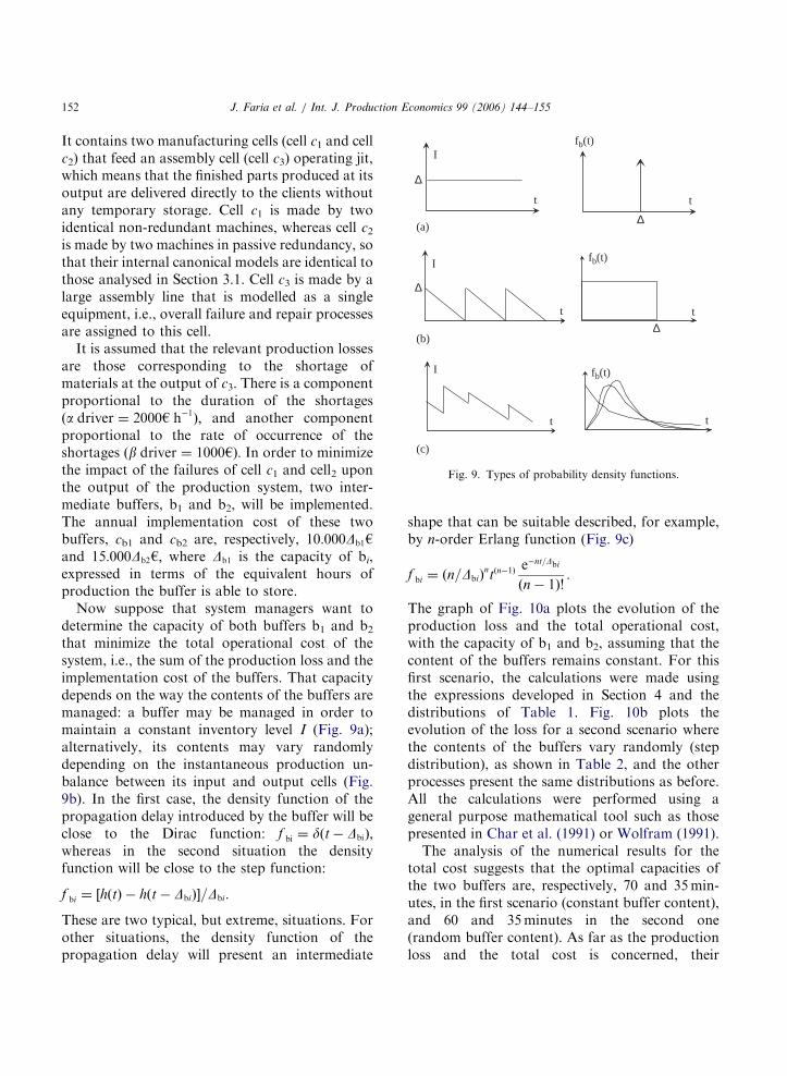
Now suppose that system managers want todetermine the capacity of both buffers b1 and b2

that minimize the total operational cost of thesystem, i.e., the sum of the production loss and theimplementation cost of the buffers. That capacitydepends on the way the contents of the buffers aremanaged: a buffer may be managed in order tomaintain a constant inventory level I (Fig. 9a);alternatively, its contents may vary randomlydepending on the instantaneous production un-balance between its input and output cells (Fig.9b). In the first case, the density function of thepropagation delay introduced by the buffer will beclose to the Dirac function: f bi ¼ dðt � DbiÞ;whereas in the second situation the densityfunction will be close to the step function:

f bi ¼ ½hðtÞ � hðt � DbiÞ�=Dbi:

These are two typical, but extreme, situations. Forother situations, the density function of thepropagation delay will present an intermediate

shape that can be suitable described, for example,by n-order Erlang function (Fig. 9c)

f bi ¼ ðn=DbiÞntðn�1Þ e�nt=Dbi

ðn � 1Þ!:

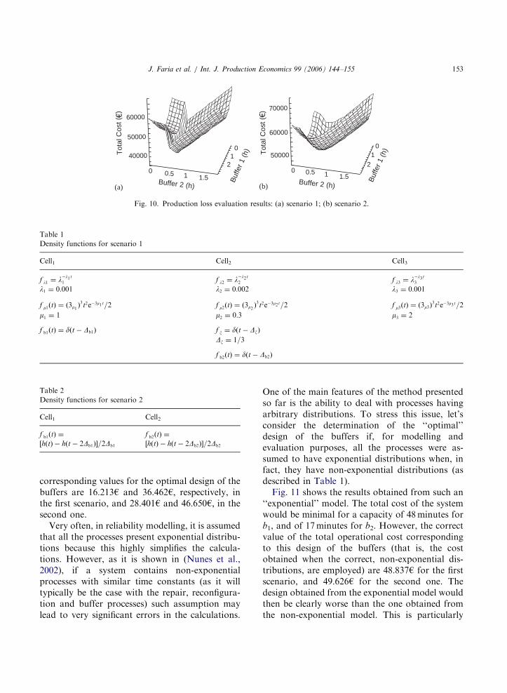
The graph of Fig. 10a plots the evolution of theproduction loss and the total operational cost,with the capacity of b1 and b2, assuming that thecontent of the buffers remains constant. For thisfirst scenario, the calculations were made usingthe expressions developed in Section 4 and thedistributions of Table 1. Fig. 10b plots theevolution of the loss for a second scenario wherethe contents of the buffers vary randomly (stepdistribution), as shown in Table 2, and the otherprocesses present the same distributions as before.All the calculations were performed using ageneral purpose mathematical tool such as thosepresented in Char et al. (1991) or Wolfram (1991).

The analysis of the numerical results for thetotal cost suggests that the optimal capacities ofthe two buffers are, respectively, 70 and 35 min-utes, in the first scenario (constant buffer content),and 60 and 35 minutes in the second one(random buffer content). As far as the productionloss and the total cost is concerned, their

ARTICLE IN PRESS

0

2

1 1.5

50000

60000

40000

60000

70000

50000

0 0.5

1

01

20 0.5 1 1.5

(a) (b)

Tot

al C

ost (

)

Tot

al C

ost (

)

Buf

fer 1

(h)

Buf

fer 1

(h)

Buffer 2 (h)Buffer 2 (h)

Fig. 10. Production loss evaluation results: (a) scenario 1; (b) scenario 2.

Table 1

Density functions for scenario 1

Cell1 Cell2 Cell3

f l1 ¼ l�l1 t

1 f l2 ¼ l�l2 t

2 f l3 ¼ l�l3 t

3

l1 ¼ 0:001 l2 ¼ 0:002 l3 ¼ 0:001

f m1ðtÞ ¼ ð3m1Þ3t2e�3m1 t=2 f m2ðtÞ ¼ ð3m2

Þ3t2e�3m2 t=2 f m3ðtÞ ¼ ð3m3Þ

3t2e�3m3 t=2

m1 ¼ 1 m2 ¼ 0:3 m3 ¼ 2

f b1ðtÞ ¼ dðt � Db1Þ f x ¼ dðt � DxÞ

Dx ¼ 1=3

f b2ðtÞ ¼ dðt � Db2Þ

Table 2

Density functions for scenario 2

Cell1 Cell2

f b1ðtÞ ¼

½hðtÞ � hðt � 2Db1Þ�=2Db1

f b2ðtÞ ¼

½hðtÞ � hðt � 2Db2Þ�=2Db2


corresponding values for the optimal design of thebuffers are 16:213h and 36:462h; respectively, inthe first scenario, and 28:401h and 46:650h; in thesecond one.

Very often, in reliability modelling, it is assumedthat all the processes present exponential distribu-tions because this highly simplifies the calcula-tions. However, as it is shown in (Nunes et al.,2002), if a system contains non-exponentialprocesses with similar time constants (as it willtypically be the case with the repair, reconfigura-tion and buffer processes) such assumption maylead to very significant errors in the calculations.

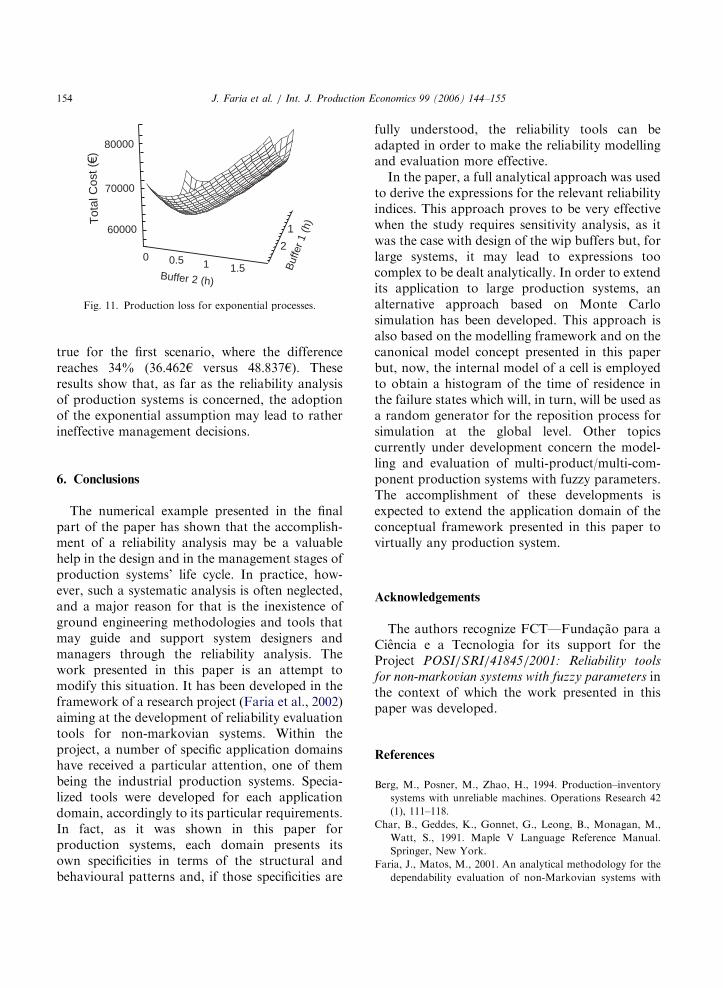
One of the main features of the method presentedso far is the ability to deal with processes havingarbitrary distributions. To stress this issue, let’sconsider the determination of the ‘‘optimal’’design of the buffers if, for modelling andevaluation purposes, all the processes were as-sumed to have exponential distributions when, infact, they have non-exponential distributions (asdescribed in Table 1).

Fig. 11 shows the results obtained from such an‘‘exponential’’ model. The total cost of the systemwould be minimal for a capacity of 48 minutes forb1, and of 17 minutes for b2. However, the correctvalue of the total operational cost correspondingto this design of the buffers (that is, the costobtained when the correct, non-exponential dis-tributions, are employed) are 48:837h for the firstscenario, and 49:626h for the second one. Thedesign obtained from the exponential model wouldthen be clearly worse than the one obtained fromthe non-exponential model. This is particularly

ARTICLE IN PRESS

70000

80000

60000 1

20 0.5 1 1.5

Tot

al C

ost (

)

Buf

fer

1 (h

)

Buffer 2 (h)

Fig. 11. Production loss for exponential processes.


true for the first scenario, where the differencereaches 34% (36:462h versus 48:837h). Theseresults show that, as far as the reliability analysisof production systems is concerned, the adoptionof the exponential assumption may lead to ratherineffective management decisions.

6. Conclusions

The numerical example presented in the finalpart of the paper has shown that the accomplish-ment of a reliability analysis may be a valuablehelp in the design and in the management stages ofproduction systems’ life cycle. In practice, how-ever, such a systematic analysis is often neglected,and a major reason for that is the inexistence ofground engineering methodologies and tools thatmay guide and support system designers andmanagers through the reliability analysis. Thework presented in this paper is an attempt tomodify this situation. It has been developed in theframework of a research project (Faria et al., 2002)aiming at the development of reliability evaluationtools for non-markovian systems. Within theproject, a number of specific application domainshave received a particular attention, one of thembeing the industrial production systems. Specia-lized tools were developed for each applicationdomain, accordingly to its particular requirements.In fact, as it was shown in this paper forproduction systems, each domain presents itsown specificities in terms of the structural andbehavioural patterns and, if those specificities are

fully understood, the reliability tools can beadapted in order to make the reliability modellingand evaluation more effective.

In the paper, a full analytical approach was usedto derive the expressions for the relevant reliabilityindices. This approach proves to be very effectivewhen the study requires sensitivity analysis, as itwas the case with design of the wip buffers but, forlarge systems, it may lead to expressions toocomplex to be dealt analytically. In order to extendits application to large production systems, analternative approach based on Monte Carlosimulation has been developed. This approach isalso based on the modelling framework and on thecanonical model concept presented in this paperbut, now, the internal model of a cell is employedto obtain a histogram of the time of residence inthe failure states which will, in turn, will be used asa random generator for the reposition process forsimulation at the global level. Other topicscurrently under development concern the model-ling and evaluation of multi-product/multi-com-ponent production systems with fuzzy parameters.The accomplishment of these developments isexpected to extend the application domain of theconceptual framework presented in this paper tovirtually any production system.

Acknowledgements

The authors recognize FCT—Fundac- ao para aCiencia e a Tecnologia for its support for theProject POSI/SRI/41845/2001: Reliability tools

for non-markovian systems with fuzzy parameters inthe context of which the work presented in thispaper was developed.

References

Berg, M., Posner, M., Zhao, H., 1994. Production–inventory

systems with unreliable machines. Operations Research 42

(1), 111–118.

Char, B., Geddes, K., Gonnet, G., Leong, B., Monagan, M.,

Watt, S., 1991. Maple V Language Reference Manual.

Springer, New York.

Faria, J., Matos, M., 2001. An analytical methodology for the

dependability evaluation of non-Markovian systems with

ARTICLE IN PRESS


multiple components. Journal of Reliability Engineering

and System Safety 74, 193–210.

Faria, J., Matos, M., Nunes, E., 2002. Reliability tools for non-

markovian systems with fuzzy parameters. Project POSI/

SRI/41845/2001, Fundac- ao para a Ciencia e a Tecnologia,

http://sifeup.fe.up.pt/sifeup/, June 2002.

Giordano, M., Martinelli, F., 2002. Optimal safety stock for

unreliable, finite buffer, single machine manufacturing

systems. IEEE International Conference on Robotics and

Automation, Washington, USA, vol. 3, May 2002,

pp. 2339–2344.

Mahadevan, B., Narendran, T., 1993. Buffer levels and choice of

material handling device in Flexible Manufacturing Systems.

European Journal of Operational Research 69, 166–176.

Moinzadeh, K., Aggarwal, P., 1997. Analysis of a production/

inventory system subject to random disruptions. Manage-

ment Science 43 (11), 1577–1588.

Nunes, E., Faria, J.A., Matos, M.A., 2002. A comparative

analysis of dependability assessment methodologies. Pro-

ceedings of the lm13 ESREL Conference, Lyon, France,

May 2002.

Van Ryzin, G., Lou, S., Gershwin, S., 1993. Production control

for tandem two-machines system. Transactions of the

Institute of Electrical Engineers 25 (5), 5–20.

Wolfram, S., 1991. Mathematic: A System for Doing

Mathematics by Computer, second ed. Addison-Wesley,

Reading, MA.

http://sifeup.fe.up.pt/sifeup/

Documents

Optimal design of work-in-process buffers