Optimal Design of Shell-and-Tube Heat Exchangers by Different Strategies of Differential Evolution

B. V. Babu* and S. A. Munawar

Department of Chemical Engineering Birla Institute of Technology and Science

PILANI-333 031 Rajasthan, India.

Abstract

This paper presents the application of Differential Evolution (DE) for the optimal design of shell-and-tube heat exchangers. The main objective in any heat exchanger design is the estimation of the minimum heat transfer area required for a given heat duty, as it governs the overall cost of the heat exchanger. Lakhs of configurations are possible with various design variables such as outer diameter, pitch, and length of the tubes; tube passes; baffle spacing; baffle cut etc. Hence the design engineer needs an efficient strategy in searching for the global minimum. In the present study for the first time DE, an improved version of Genetic Algorithms (GAs), has been successfully applied with different strategies for 1,61,280 design configurations using Bell�s method to find the heat transfer area. In the application of DE 9680 combinations of the key parameters are considered. For comparison, GAs are also applied for the same case study with 1080 combinations of its parameters. For this optimal design problem, it is found that DE, an exceptionally simple evolution strategy, is significantly faster compared to GA and yields the global optimum for a wide range of the key parameters. Keywords: Shell-and-Tube Heat Exchanger; Heat Exchanger Design; Optimization; Evolutionary Computation; Genetic Algorithms; Differential Evolution ______________________________________________________________________________________________________________________

1. Introduction

The transfer of heat to and from process fluids is an essential part of most of the chemical processes. Therefore, Heat Exchangers (HEs) are used extensively and regularly in process and allied industries and are very important during design and operation. The most commonly used type of heat exchanger is the shell-and-tube heat exchanger, the optimal design of which is the main objective of this study. Computer software marketed by companies such as HTRI and HTFS are used extensively in the thermal design and rating of HEs. These packages incorporate various design options for the heat exchangers including the variations in the tube diameter, tube pitch, shell type, number of tube passes, baffle spacing, baffle cut, etc.

A primary objective in the Heat Exchanger Design (HED) is the estimation of the minimum heat transfer area required for a given heat duty, as it governs the overall cost of the HE. But there is no concrete objective function that can be expressed explicitly as a function of the design

*Corresponding author: Group Leader, Engineering Technology Group, Engineering Services Division

E-mail: bvbabu@bits-pilani.ac.in; Fax: 0091 1596 44183; Ph: 0091 1596 45073 Ext. 205

variables and in fact many number of discrete combinations of the design variables are possible as is elaborated below. The tube diameter, tube length, shell types etc. are all standardized and are available only in certain sizes and geometry. And so the design of a shell-and-tube heat exchanger usually involves a trial and error procedure where for a certain combination of the design variables the heat transfer area is calculated and then another combination is tried to check if there is any possibility of reducing the heat transfer area. Since several discrete combinations of the design configurations are possible, the designer needs an efficient strategy to quickly locate the design configuration having the minimum heat exchanger cost. Thus the optimal design of heat exchanger can be posed as a large scale, discrete, combinatorial optimization problem (Chaudhuri et al., 1997).

Most of the traditional optimization techniques based on gradient methods have the possibility of getting trapped at local optimum depending upon the degree of non-linearity and initial guess. Hence, these traditional optimization techniques do not ensure global optimum and also have limited applications. In the recent past, some expert systems based on natural phenomena (Evolutionary Computation) such as Simulated Annealing (Kirkpatrick et al., 1983) and Genetic Algorithms (Goldberg, 1989; Davis, 1991) have been developed to overcome this problem.

Simulated Annealing (SA) is a probabilistic nontraditional optimization technique, which resembles the thermodynamic process of cooling of molten metals to achieve the minimum energy state. Rutenbar (1989) gave a detailed discussion of the working principle of SA and its applications. SA has diffused widely into many diverse applications. The various applications of SA include: traveling salesman problem (Cerny, 1985; Allwright & Carpenter, 1989), scheduling of serial multi-component batch processes (Das et al., 1990), heat exchanger network synthesis (Dolan et al., 1990; Athier et al., 1997a & 1997b), preliminary design of multi-product non-continuous plants (Patel et al., 1991), separation sequence synthesis (Floquet et al., 1994), synthesis of utility systems (Maia et al., 1995), reactor networks synthesis (Cordero et al., 1997) etc.

Genetic Algorithms (GA) are computerized search and optimization algorithms based on the mechanics of natural genetics and natural selection. They mimic the �survival of the fittest� principle of nature to make a search process. The key parameters of control in GA are: N, the population size; pc, the crossover probability; and pm, the mutation probability (Goldberg, 1989; Deb, 1996). Since their inception, GAs have evolved like the species they try to mimic and have been applied successfully in many diverse fields. The various applications of GAs are: process design and optimization (Androulakis & Venkatasubramanian, 1991), computer-aided molecular design (Venkatasubramanian et al., 1994), heat integrated processes (Stair & Fraga, 1995), parameter estimations for kinetic models of catalytic processes (Moros et al., 1996), optimal design of ammonia synthesis reactor (Upreti & Deb, 1996), on-line optimization of culture temperature for ethanol fermentation (Moriyama & Shimizu, 1996), synthesis and optimization of non-ideal distillation system (Fraga & Senos Matias, 1996), estimating rate constants of heterogeneous catalytic reactions (Wolf & Moros, 1997), molecular scale catalyst design (Mcleod et al., 1997), estimation of heat transfer parameters in trickle bed reactors (Babu & Vivek, 1999) etc.

Chaudhuri et al., (1997) used Simulated Annealing for the optimal design of heat exchangers and developed a command procedure, to run the HTRI design program coupled to the annealing algorithm, iteratively. They have compared the results of the SA program with a base case design and concluded that significant savings in the heat transfer area and hence the HE cost can be obtained using SA. Manish et al., (1999) used a genetic algorithm framework to solve this optimal problem of HED along with SA and compared the performance of SA and GAs in solving this problem. They also presented GA strategies to improve the performance of the optimization framework. They concluded that these algorithms result in considerable savings in computational time compared to an exhaustive search, and have an advantage over other methods in obtaining multiple solutions of the same quality, thus providing more flexibility to the designer.

This paper demonstrates the first successful application of Differential Evolution, an improved version of GA, to the optimal heat exchanger design problem. Differential Evolution (DE), a recent optimization technique, is an exceptionally simple evolution strategy that is significantly faster and robust at numerical optimization and is more likely to find a function�s true global optimum (Price & Storn, 1997). Unlike simple GA that uses a binary coding for representing problem parameters, DE uses real coding of floating point numbers. The mutation operator here is addition instead of bit-wise flipping used in GA. And DE uses non-uniform crossover and tournament selection operators to create new solution strings. Among the DE�s advantages are its simple structure, ease of use, speed and robustness. It can be used for optimizing functions with real variables and many local optima.

In the recent past, DE has been successfully used in various diverse fields: digital filter design (Storn, 1995), neural network learning (Masters & Land, 1997), fuzzy-decision-making problems of fuel ethanol production (Wang et al., 1998), design of fuzzy logic controllers (Sastry et al., 1998), batch fermentation process (Chiou & Wang, 1999; Wang & Cheng, 1999), multi-sensor fusion (Joshi & Sanderson, 1999), dynamic optimization of continuous polymer reactor (Lee et al., 1999) etc. DE can also be used for parameter estimations. Babu & Sastry (1999) used DE for the estimation of effective heat transfer parameters in trickle-bed reactors using radial temperature profile measurements. They concluded that DE takes less computational time to converge compared to the existing techniques without compromising on the accuracy of the parameter estimates.

In our earlier study, we have used DE for the same optimal problem of shell-and-tube HED but with only the usual DE/rand/1/bin strategy (Babu & Munawar, 2000). In the present study, all the ten different strategies of DE (Price and Storn, 2000) are explored to suggest the best suitable strategy for this optimal problem. Also for each strategy the best DE key parameter combinations are suggested for this problem along with the suitable seed for the pseudo random number generator. The objectives of the present study are: (1) Application of DE for a case study taken up, for the optimal design of a shell-and-tube heat exchanger, with the results of a proprietary program for the same optimal design, as the base case, (2) Application of various DE strategies for this case study with a generalized pressure drop constraint, and (3) comparison of the results with GA.

In the next section, the general procedure of shell-and-tube heat exchanger design is discussed followed by the optimal problem formulation. In this study, Bell�s method is used to find the heat transfer area for a given design configuration along with the pressure drop constraint. An exhaustive search will require 1,61,280 function evaluations to locate the global minimum heat exchanger cost. For the case study taken up, all the ten different strategies of DE are applied over a wide range of the key parameter combinations considered. The performance of DE and GA is compared with respect to some criteria identified and defined in this study. It is found that DE, an exceptionally simple evolution strategy is significantly faster compared to GA, yields the global optimum over a wide range of the key parameters and proves to be a potential source for accurate and faster optimization.

2. The Optimal HED problem

The proper use of basic heat transfer knowledge in the design of practical heat transfer equipment is an art. The designer must be constantly aware of the differences between the idealized conditions for which the basic knowledge was obtained versus the real conditions of the mechanical expression of his design and its environment. The result must satisfy process and operational requirements (such as availability, flexibility, and maintainability) and do so economically. Heat exchanger design is not a highly accurate art under the best of conditions (Perry & Green, 1993).

2.1. Generalized Design Procedure for Heat Exchangers

The design of a process heat exchanger usually proceeds through the following steps (Perry & Green, 1993):

• Process conditions (stream compositions, flow rates, temperatures, pressures) must be specified. • Required physical properties over the temperature and pressure ranges of interest must be obtained. • The type of heat exchanger to be employed is chosen. • A preliminary estimate of the size of the exchanger is made, using a heat transfer coefficient appropriate

to the fluids, the process, and the equipment. • A first design is chosen, complete in all details necessary to carryout the design calculations. • The design chosen is now evaluated or rated, as to its ability to meet the process specifications with

respect to both heat duty and pressure drop. • Based on this result a new configuration is chosen if necessary and the above step is repeated. If the first

design was inadequate to meet the required heat load, it is usually necessary to increase the size of the exchanger, while still remaining within specified or feasible limits of pressure drop, tube length, shell diameter, etc. This will sometimes mean going to multiple exchanger configurations. If the first design more than meets heat load requirements or does not use all the allowable pressure drop, a less expensive exchanger can usually be designed to fulfil process requirements.

• The final design should meet process requirements (within the allowable error limits) at lowest cost. The lowest cost should include operation and maintenance costs and credit for ability to meet long-term process changes as well as installed (capital) cost. Exchangers should not be selected entirely on a lowest first cost basis, which frequently results in future penalties.

The flow chart given in Fig. 1 (Sinnott, 1993) gives the sequence of steps and the loops involved in the optimal design of a shell-and-tube heat exchanger.

Fig. 1

2.2. The optimal problem formulation

The objective function and the optimal problem of shell-and-tube HED of the present study are represented as shown in Table-1, similar to the problem formulation of Manish et al., (1999).

Table-1

The objective function can be minimization of HE cost C(X) or heat transfer area A(X) and X is a solution string representing a design configuration. The design variable x1 takes 12 values for tube outer diameter in the range of 0.25� to 2.5� (0.25�, 0.375�, 0.5�, 0.625�, 0.75�, 0.875�, 1.0�, 1.25�, 1.5�, 1.75�, 2�, 2.5�). x2 represents the tube pitch - either square or triangular - taking two values represented by 1 and 2. x3 takes the shell head types: floating head, fixed tube sheet, U tube, and pull through floating head represented by the numbers 1, 2, 3 and 4 respectively. x4 takes number of tube passes 1-1, 1-2, 1-4, 1-6, 1-8 represented by numbers from 1 to 5. The variable x5 takes eight values of the various tube lengths in the range 6� to 24� (6�, 8�, 10�, 12�, 16�, 20�, 22�, 24�) represented by numbers 1 to 8. x6 takes six values for the variable baffle spacing, in the range 0.2 to 0.45 times the shell diameter (0.2, 0.25, 0.3, 0.35, 0.4, 0.45). x7 takes seven values for the baffle cut in the range 15 to 45 percent (0.15, 0.2, 0.25, 0.3, 0.35, 0.4, 0.45).

In the present study, the pressure drop on the fluids exchanging heat is considered to be the feasibility constraint. Generally a pressure drop of more than 1 bar is not desirable for the flow of fluid through a HE. For a given design configuration, whenever the pressure drop exceeds the specified limit, a high value for the heat transfer area is returned so that as an infeasible configuration it will be eliminated in the next

iteration of the optimization routine. The total number of design combinations with these variables are 12 x 2 x 4 x 5 x 8 x 6 x 7 = 1,61,280. This means that if an exhaustive search is to be performed it will take at the maximum 1,61,280 function evaluations before arriving at the global minimum heat exchanger cost. So the strategy which takes few function evaluations is the best one. Considering minimization of heat transfer area as the objective function, differential evolution technique is applied to find the optimum design configuration with pressure drop as the constraint. For the case study considered, the performance of DE is compared with GA and the results are discussed in the fourth section.

3. Differential evolution: at a glance

We all must accept that �Nature knows the best!� and we, the human beings try to mimic nature and its natural phenomenon in our efforts for the development of technology and resources. Few of the outcomes of such efforts are the evolution of nontraditional optimization techniques (Evolutionary computation) such as Simulated Annealing (SA), Genetic Algorithms (GA), and Differential Evolution (DE). In the recent past, these algorithms have been successfully applied for solving complex engineering optimization problems and are widely known to diffuse very close to the global optimum solution.

A genetic algorithm that is well adapted to solving a combinatorial task like the traveling salesman problem may fail miserably when used to minimize functions with real variables and many local optima. The concept of binary coding used by simple GA limits the resolution with which an optimum can be located to the precision set by the number of bits in the integer. So, the simple GA was later modified to work with the real variables as well. Just as floating point numbers are more appropriate than integers for representing points in continuous space, addition is more appropriate than random bit flipping for searching the continuum (Price & Storn, 1997). Consider, for example to change a binary 16 (10000) into a binary 15 (01111) with bit-wise flipping would require inverting all the five bits. In most bit flipping schemes a mutation of this magnitude would be rare. Alternately under addition, 16 become 15 simply by adding -1. Adopting addition as the mutation operator to restore the adjacency of nearby points is not, however, a panacea. Then the fundamental question concerning addition would be how much to add. The simple adaptive scheme used by DE ensures that these mutation increments are automatically scaled to the correct magnitude. Similarly DE uses a non-uniform crossover in that the parameter values of the child vector are inherited in unequal proportions from the parent vectors. For reproduction, DE uses a tournament selection where the child vector competes against one of its parents.

The overall structure of the DE algorithm resembles that of most other population based searches. The parallel version of DE maintains two arrays, each of which holds a population of NP, D-dimensional, real valued vectors. The primary array holds the current vector population, while the secondary array accumulates vectors that are selected for the next generation. In each generation, NP competitions are held to determine the composition of the next generation. Every pair of vectors ( Xa, Xb ) defines a vector differential: Xa - Xb. When Xa and Xb are chosen randomly, their weighted differential is used to perturb another randomly chosen vector Xc. This process can be mathematically written as X'

c = Xc + F ( Xa - Xb ). The scaling factor F is a user supplied constant in the range (0 < F ≤ 1.2). The optimal value of F for most of the functions lies in the range of 0.4 to 1.0 (Price & Storn, 1997). Then in every generation, each primary array vector, Xi is targeted for crossover with a vector like X'

c to produce a trial vector Xt. Thus the trial vector is the child of two parents, a noisy random vector and the target vector against which it must compete. The non-uniform crossover is used with a crossover constant CR, in the range 0 ≤ CR ≤ 1. CR actually represents the probability that the child vector inherits the parameter values from the noisy random vector. When CR = 1, for example, every trial vector parameter is certain to come from X'

c. If, on the other hand, CR=0, all but one trial vector parameter comes from the target vector. To ensure that Xt differs from Xi by at least one parameter, the final trial vector parameter always comes from the noisy random vector, even when CR = 0. Then the cost of the trial vector is compared with that of the target vector, and the vector

that has the lowest cost of the two would survive for the next generation. In all, just three factors control evolution under DE, the population size, NP; the weight applied to the random differential, F; and the crossover constant, CR.

3.1. Different strategies of DE

Different strategies can be adopted in DE algorithm depending upon the type of problem for which DE is applied. The strategies can vary based on the vector to be perturbed, number of difference vectors considered for perturbation, and finally the type of crossover used. The following are the ten different working strategies proposed by Price & Storn (2000):

1. DE/best/1/exp 2. DE/rand/1/exp 3. DE/rand-to-best/1/exp 4. DE/best/2/exp 5. DE/rand/2/exp 6. DE/best/1/bin 7. DE/rand/1/bin 8. DE/rand-to-best/1/bin 9. DE/best/2/bin 10. DE/rand/2/bin

The general convention used above is DE/x/y/z. DE stands for Differential Evolution, x represents a string denoting the vector to be perturbed, y is the number of difference vectors considered for perturbation of x, and z stands for the type of crossover being used (exp: exponential; bin: binomial). Thus, the working algorithm outlined above is the seventh strategy of DE i.e. DE/rand/1/bin. Hence the perturbation can be either in the best vector of the previous generation or in any randomly chosen vector. Similarly for perturbation either single or two vector differences can be used. For perturbation with a single vector difference, out of the three distinct randomly chosen vectors, the weighted vector differential of any two vectors is added to the third one. Similarly for perturbation with two vector differences, five distinct vectors, other than the target vector are chosen randomly from the current population. Out of these, the weighted vector difference of each pair of any four vectors is added to the fifth one for perturbation. In exponential crossover, the crossover is performed on the D variables in one loop until it is within the CR bound. The first time a randomly picked number between 0 and 1 goes beyond the CR value, no crossover is performed and the remaining D variables are left intact. In binomial crossover, the crossover is performed on each of the D variables whenever a randomly picked number between 0 and 1 is within the CR value. So for high values of CR, the exponential and binomial crossovers yield similar results. The strategy to be adopted for each problem is to be determined separately by trial and error. A strategy that works out to be the best for a given problem may not work well when applied for a different problem.

3.2. Choosing NP, F, and CR

Choosing NP, F, and CR depends on the specific problem applied, and is often difficult. But some general guidelines are available. Normally, NP should be about 5 to 10 times the number of parameters in a vector. As for F, it lies in the range 0.4 to 1.0. Initially F = 0.5 can be tried then F and/or NP is increased if the population converges prematurely. A good first choice for CR is 0.1, but in general CR should be as large as possible (Price & Storn, 1997). The best combination of these key parameters of DE for each of the strategies mentioned earlier is again different. Price & Storn (2000) have mentioned some simple rules for choosing the best strategy as well as the corresponding key parameters. Among DE�s advantages are its simple structure, ease of use, speed and robustness. Already, DE has been successfully applied for solving

several complex problems and is now being identified as a potential source for accurate and faster optimization.

4. Results and discussions

The algorithm of Differential Evolution as given by Price and Storn (2000), is in general applicable for continuous function optimization. The upper and lower bounds of the design variables are initially specified. Then, after mutation because of the addition of the weighted random differential the parameter values may even go beyond the specified boundary limits. So, irrespective of the boundary limits initially specified, DE finds the global optimum by exploring beyond the limits. Hence, when applied to discrete function optimization the parameter values have to be limited to the specified bounds. In the present problem, since each design variable has a different upper bound when represented by means of integers, the same DE code given by Price and Storn (2000) cannot be used. We have used the normalized values for all the design variables and randomly initialized all the design variables between 0 and 1. Whenever it is required to find the heat transfer area using Bell�s method for a given design configuration, these normalized values are converted back to their corresponding boundary limits. The pseudo code of the DE algorithm used in the present study for the optimal heat exchanger design problem is given below:

• Choose a strategy and a seed for the random number generator. • Initialize the values of D, NP, CR, F and MAXGEN. • Initialize all the vectors of the population randomly. Since the upper bounds are all different for each variable in

this problem, the variables are all normalized. Hence generate a random number between 0 and 1 for all the design variables for initialization.

for i = 1 to NP { for j = 1 to D xi,j = random number } • Evaluate the cost of each vector. Cost here is the area of the shell-and-tube heat exchanger for the given design

configuration, calculated by a separate function cal_area() using Bell� method. for i = 1 to NP

Ci = cal_area() • Find out the vector with the lowest cost i.e. the best vector so far. Cmin = C1 and best =1 for i = 2 to NP { if (Ci < Cmin) then Cmin = Ci and best = i } • Perform mutation, crossover, selection and evaluation of the objective function for a specified number of

generations. While (gen < MAXGEN) { for i = 1 to NP { • For each vector Xi (target vector), select three distinct vectors Xa, Xb and Xc (select five, if two vector differences

are to be used) randomly from the current population (primary array) other than the vector Xi do

{ r1 = random number * NP r2 = random number * NP r3 = random number * NP } while (r1 = i) OR (r2 = i) OR (r3 = i) OR (r1 = r2) OR (r2 = r3) OR (r1 = r3) • Perform crossover for each target vector Xi with its noisy vector Xn,i and create a trial vector, Xt,i. The noisy vector

is created by performing mutation. If CR = 0 inherit all the parameters from the target vector Xi, except one which should be from Xn,i.

for exponential crossover { p = random number * 1 r = random number * D n = 0 do

{ Xn, i = Xa, i + F ( X b, i - X c, i ) /* add two weighted vector differences for r = ( r+1 ) % D two vector perturbation. For best / random

increment r by 1 vector perturbation the weighted vector } while ( ( p<CR ) and ( r<D ) ) difference is added to the best / random vector of the current population. */

} for binomial crossover { p = random number * 1

r = random number * D for n = 1 to D { if ( ( p<CR ) or ( p = D-1 ) ) /* change at least one parameter if CR=0 */ Xn, i = Xa, i + F ( X b, i - X c, i ) r = (r+1)%D }

} if ( Xn, i > 1 ) Xn, i = 1 /* for discrete function optimization check the if ( Xn, i < 0 ) Xn, i = 0 values to restrict to the limits */

/* 1 - normalized upper bound; 0 � normalized lower bound */

• Perform selection for each target vector, Xi by comparing its cost with that of the trial vector, Xt,i ; whichever has the lowest cost will survive for the next generation.

Ct,i = cal_area() if ( Ct,i < Ci ) new Xi = Xt,i

else new Xi = X i } /* for i=1 to NP */ } • Print the results.

The entire scheme of optimization of shell-and-tube heat exchanger design is performed by the DE algorithm, while intermittently it is required to evaluate the heat transfer area for a given design configuration. This task is accomplished through the separate function cal_area() which employs Bell�s method of heat exchanger design. Bell�s method gives accurate estimates of the shell-side heat transfer coefficient and pressure drop compared to Kern's method, as it takes into account the factors for leakage, bypassing, flow in window zone etc. The various correction factors in Bell�s method include: temperature correction factor, tube-side heat transfer and friction factor, shell-side heat transfer and friction factor, tube row correction factor, window correction factor for heat transfer and pressure drop, bypass correction factor for heat transfer and pressure drop, friction factor for cross-flow tube banks, baffle geometrical factors etc. These correction factors are reported in the literature in the form of nomographs (Sinnott, 1993; Perry & Green, 1993). In the present study, the data on these correction factors from the nomographs are fitted into polynomial equations and incorporated in the computer program.

As a case study the following problem for the design of a shell-and-tube heat exchanger (Sinnott, 1993) is considered:

20,000 kg/hr of kerosene leaves the base of a side-stripping column at 200oC and is to be cooled to 90oC with 70,000 kg/hr light crude oil coming from storage at 40oC. The kerosene enters the exchanger at a pressure of 5 bar and the crude oil at 6.5 bar. A pressure drop of 0.8 bar is permissible on both the streams. Allowance should be made for fouling by including fouling factor of 0.00035 (W/m2 0C)�1 on the crude stream and 0.0002 (W/m2 0C)�1 on the kerosene side.

By performing the enthalpy balance, the heat duty for this case study is found to be 1509.4 kW and the outlet temperature of crude oil to be 78.6oC. The crude is dirtier than the kerosene and so is assigned through the tube-side and kerosene to the shell-side. Using a proprietary program (HTFS, STEP5) the lowest cost design meeting the above specifications is reported to be a heat transfer area of 55 m2 based on outside diameter (Sinnott, 1993). Considering the result of the above program as the base case design, in the present study DE is applied for the same problem with all the ten different strategies.

As a heuristic, the pressure drop in a HE normally should not exceed 1 bar. Hence, the DE strategies are applied for this case study separately with both 0.8 bar and 1 bar as the constraints. In both the cases, the same global minimum heat exchanger area of 34.44 m2 is obtained using DE as against 55 m2 reported by Sinnott, 1993. But, in the subsequent analysis, the results for 1 bar as the constraint are referred here in drawing the generalized conclusions.

A seed value for the pseudo random number generator should be selected by trial and error. In principle any positive integer can be taken. Integers 3, 5, 7, 10, 15 and 20 are tried with all the strategies for a NP value of 70 (10 times D). The F values are varied from 0.1 to 1.1 in steps of 0.1 and CR values from 0 to 1 in steps of 0.1, leading to 121 combinations of F and CR for each seed. When DE program is executed for all the above combinations, the global minimum HE area for the above heat duty is found to be 34.44 m2 as against 55 m2 for the base case design � indicating that DE is likely to converge to the true global optimum. For each seed, out of the 121 combinations of F and CR considered, the percentage of the combinations converging to this global minimum (CDE) in less than 30 generations is listed for each strategy in Table-2. The average CDE for each seed as well as for each strategy are also listed in Table-2. This average can be considered to be a measure of the likeliness in achieving the global minimum.

Table-2

From this table it is evident that the individual values of CDE cover a wide range from 28.1 to 81.8 - indicating that DE is more likely to find the global optimum. Combining this above observation with the earlier one, it can be concluded that DE is more likely to find a function�s true global optimum compared to the base case design. The average CDE for each seed ranges from 40.7 to 64.8. In this range, the average CDE for seeds 5, 7 and 10 is above 54 and so these seeds are good relative to others. With a benchmark of 40 for the individual CDE values as well, seeds 5, 7 and 10 stand good from the rest. Thus with these seeds, there is more likeliness of achieving the global minimum. Whereas with seeds 3, 5 and 20 there are more of CDE values below 40 and hence not considered to be good from likeliness point of view.

The average CDE for different strategies varies from 44.2 to 59.4 and hence all are good if an average CDE of 40 is considered to be the benchmark. With the same benchmark for CDE values also is taken, then, excepting strategy numbers 2, 7 and 8 all other strategies are good. Considering �speed � as the other criteria, to further consolidate the effect of strategies on each seed and vice versa, the best combinations of F and CR - taking the minimum number of generations to converge to the global minimum (Gmin) - are listed in Table-3.

Table-3

The Criteria for choosing a good seed from �speed� point view could be: (1) It should yield the global minimum in less number of generations, and (2) It should yield the same over a wide range of F and CR for most of the strategies. Following the first criteria with a benchmark of - achieving the global minimum in not more than two generations � seed 3 is eliminated. Satisfying the second criteria also, only seeds 7 and 10 remain. But comparing the overall performance of seeds 7 and 10, seed 10 yields the global minimum in two generations for more number of combinations of F and CR (18 times) than for seed 7 (11 times). Also, when random numbers are generated between 1 and 10 using seed 10, it is observed that it generates more 1�s which is required in the design configuration leading to the global minimum. Though seed 5 was good from the �more likeliness� point of view (from Table-2), but with �speed� as the other criteria it got eliminated. Similarly with seed 15, using DE/rand/2/exp, with F = 0.6 and CR = 0.9, though the global minimum is achieved in one generation itself, still it is not considered as more number of generations are taken to converge with other strategies and other combinations of F and CR. From the �speed� point of view it can be observed from Table-3 that the strategy numbers 2, 5, 7, and 10 are good. Hence, from both �more likeliness� and �speed� point of view, for different seeds, strategy numbers 1, 3, 4, 6, and 9 are good.

From the above results, it is also observed that, if for a given seed the random numbers generated are already good, then by using DE/best/1/...(strategy numbers 1 and 6) the global minimum is achieved in few generations itself. For example, with seeds 3 and 10 the global minimum is achieved in two generations itself with DE/best/1/... strategies. To summarize the effect of seed on each strategy, from Table-3, the best seeds and the number of combinations of F and CR in which the global minimum is achieved are listed for each strategy in Table-4 along with Gmin.

Table-4

The seed value of 10 works well for four out of the ten strategies considered for a total of 19 combinations of F and CR. Seed 7 does well with 3 strategies, but for a total of 10 combinations of F and CR only. From this table also, it is clear that the seed value of 10 is better out of all the seeds considered.

Once a good seed is chosen, the next step is to study the effect of the key parameters of DE to find the best combinations of NP, F and CR for each strategy. For this, the DE algorithm for the optimal HED problem is executed for all the ten strategies for various values of NP, F and CR with MAXGEN = 15. The population size, NP is normally about five to ten times the number of parameters in a vector D (Price & Storn, 1997). To further explore the effect of the key parameters in detail, the NP values are varied from 10 to 100 in steps of 10 and F & CR values are varied again as before. The reason for taking MAXGEN = 15 can be explained as follows. As can be seen from Table-3, at the maximum 12 generations are taken to converge to the global minimum with NP=70. Hence, to study the effect of NP, the MAXGEN is restricted to only 15 so that with other NP values if more number of generations are taken then NP=70 itself can be claimed to be the best population size.

With MAXGEN = 15, and for the selected seed value of 10, the percentage of the combinations converging to the global minimum (CDE) are listed for each strategy in Table-5 for different NP values.

Table-5

Though the NP values are varied from 10 to 100, the results for NP = 10, 20, and 30 are neither shown in Table-5 nor considered in the subsequent analysis for the following reasons: (1) The global minimum is not achieved for any of the combinations of F and CR with some strategies for these NP values, and (2) To have the same basis for comparison with GA, for which the N values are varied from 32 to 100 (the reasons for taking the above range of N for GA is explained later). From this table, it is seen that the individual CDE values cover a wide range from 0.8 to 66.1. The average CDE for each NP as well as for each strategy are also listed in Table-5. This average is again a measure of the likeliness of achieving the global minimum. The average CDE for different NP varies from 6.3 to 31.3. With a benchmark of 10 for this average CDE, it can be observed that, NP value of 70 and above stand good from the rest. From �more likeliness� point of view, with a benchmark of 20 for CDE values, again NP values of 70 and above are good. But for NP values of 100 and above it is observed that the likeliness decreases. The average CDE for different strategies in Table-5 varies from 6.0 to 32.1. With a benchmark of 15 for this average CDE, from �more likeliness� point of view, strategy numbers 1, 3, 4, 6, 8, and 9 stand good from the rest.

Considering �speed� again as the other criteria, the best combinations of F and CR � taking the least number of generations to converge to the global minimum (Gmin) � are listed in Table-6, for various strategies with different NP values.

Table-6

From this table it can be seen that for certain combinations of F and CR, DE is able to converge to the global minimum in a single generation also. From the �speed� point of view also again it is evident that the NP

values of 70 and above are good � indicating that at least a population size of 10 times D is essential to have more likeliness in achieving the global minimum. It is in agreement with the simple rules proposed by Price & Storn (1997). And strategy numbers 1, 4, 6, and 9 are good. Hence, from �more likeliness� as well as �speed� point of view, for different NP values, strategy numbers 1, 4, 6, and 9 are good.

Combining the results of variations in seed and NP, from �more likeliness� as well as �speed� point of view, it can be concluded that DE/best/�(strategy numbers 1, 4, 6, and 9) are good. Hence, for this optimal HED problem, the best vector perturbations either with a single or two vector differences are the best with either exponential or binomial crossovers.

The Number of Function Evaluations (NFE) are related to the population size, NP as NFE = NP * (Gmin + 1) (plus one corresponds to the function evaluations of the initial population). It can be inferred from Table-6 (using NP and Gmin values to compute NFE) that NFE varies from only 100 to 1300, out of the 1,61,280 possible function evaluations considered. Hence, the best combination corresponding to the least function evaluations from Table-6 is for NP = 50 and DE/best/1/exp strategy, with 100 function evaluations as it converges in one generation itself. For this combination DE took 0.1 seconds of CPU time on a 266 MHz Pentium-II processor.

Now, to study the effect of F and CR on various strategies, the DE algorithm is executed for the present optimal problem, for different values of F and CR. For the selected seed value of 10 and NP = 70, the F values are varied from 0.5 to 1.0 in steps of 0.1 and CR values from 0 to 1 in steps of 0.1. For the ten different strategies considered in the above range of F and CR, 21 plots are made for number of generations versus CR values with F as a parameter; and 18 plots for the number of generations versus F values with CR as a parameter. Typical graphs are shown in Figs. 2 to 9. The numbers given in the legend correspond to the strategy. Whenever the global minimum is obtained, it is observed that DE converges in less than 70 generations for strategies 1, 4, 6, and 9; and in less than 100 generations for the rest of the strategies. This implies that for any particular combination of the key parameters, if convergence is not achieved in less than 100 generations, then it is never achieved. So the points at 100 generations in the graphs correspond to the misconvergence and hence represent local minima (other than 34.44 m2 and obviously higher values of area).

Fig. 2, 3, 4 Fig. 5, 6 Fig. 7, 8, 9

For studying the effect of F and CR on each strategy, the criterion considered is �speed�. So, it should yield the global minimum in less number of generations. In Figs. 2, 3, and 4, from the �speed� point of view, it can be seen that with F as a parameter, in general (excluding the misconvergence points) DE/best/1/...(strategy numbers 1 and 6) are better than DE/best/2/.. (strategy numbers 4 and 9) unlike from �more likeliness� point of view (Table-2 & Table-5), where DE/best/2/.. is better than DE/best/1/.. as the former one takes less number of generations. Similar trends are observed for CR also as a parameter. It means that if best vector perturbation is to be tried then, from the �speed� point of view, it is worth trying it with single vector perturbation first to see quickly if there is any convergence. If misconvergence occurs DE/best/2/.. can be tried as it has more likeliness of achieving the global minimum. With DE/best/1/.. it is observed that at low values of F binomial crossover is better than exponential crossover (Fig. 2); and as F values are increased there is no marked difference in the performance of exponential and binomial crossover. From the �speed� point of view this observation is again clearly evident from Tables-3 and 6. But for DE/best/2/.. binomial crossover seems to be better than that of exponential, as it yields the global minimum in less number of generations at medium to higher values of F (excluding the misconvergence points) (Figs. 3 and 4). This observation is also clearly evident from the �speed� point of view in Tables-3 and 6. Similar trends are observed with CR also as a parameter.

If misconvergence occurs with DE/best/..., either DE/rand-to-best/1/... or DE/rand/...seem to be the immediate good options. In Figs. 5, 6, and 9, from the �speed� point of view DE/rand/2/... is seen to be better than DE/rand/1/... at high values of F and CR. The same observation is drawn from �speed� point of view, in Tables-3 and 6 as well - indicating that if random vector perturbation is to be used then, from the �speed� point of view, it is better to use it with two vector differences. From Figs. 7 and 8, with DE/rand/1/.., exponential crossover seems to be a better option. For the optimal HED problem considered, it is concluded from the preceding discussions that for variations in seed and NP, from �more likeliness� as well as �speed� point of view DE/best/.. strategies are better than DE/rand/.. From these results it is also observed that the DE strategies are more sensitive to the values of CR than to F. Extreme values of CR are worth to be tried first. From Fig. 9 it can be observed that there is no difference in the performance of exponential and binomial crossover at CR=1.0, which is quite obvious from the nature of these operators. The priority order of the strategies to be employed for a given optimal problem may vary from what is observed above. Selection of a good seed is indeed the first hurdle before investigating the right combination of the key parameters and the choice of the strategy. Some of these observations made in present the study form the supportive evidence of the recommendations and suggestions, made for other applications by Price and Storn (2000).

For comparison, Genetic Algorithms with binary coding for the design variables are also applied for the same case study with Roulette-wheel selection, single-point crossover, and bit-wise mutation as the operators for creating the new population. The GA algorithm is executed for various values of N - the population size, pc � the crossover probability and pm � the mutation probability. With a seed value of 10 for the pseudo random number generator, N is varied from 32 to 100 in steps of 4; pc from 0.5 to 0.95 in steps of 0.05; and pm from 0.05 to 0.3 in steps of 0.05, leading to a total of 1080 combinations. The reasons for not considering the N values of 30 and below are same as those already explained for NP while discussing the results with DE. N/2 has to be an even number for single-point crossover and hence the starting value of 32 and the step size of 4 are taken. The step size is smaller for GA compared to DE, as it can be seen later that GA has less likeliness so more search space is required. For each population size, 60 combinations of pc and pm are possible in this range. For the case study considered, the same global minimum heat transfer area is obtained (34.44m2) by using GA also. The minimum number of generations required by GA to converge to the global minimum (Gmin), in the above range of the key parameters is listed in Table-7 along with the Number of Function Evaluations (NFE).

Table-7

For each combination of N and pc listed in this table, GA is converging to the global minimum heat transfer area of 34.44 m2 for all the six values of pm from 0.05 to 0.3 in steps of 0.05. While executing the GA program, it is observed that more number of generations are taken by GA to converge and hence, the maximum number of generations (MAXGEN) is specified as 100. For a given N, the percentage of the combinations converging to the global minimum (CGA) in less than 100 generations, out of the 60 possible combinations of pc and pm considered, is also listed in Table-7. As can be seen, CGA ranges from 10 to 50 only as against the individual CDE (Table-5), which varies from 0.8 to 66.1. Comparing the individual CDE range for one of the best strategy DE/best/2/bin from Table-5, which varies 11.6 to 66.1 (except one that is 3.3), CGA is relatively less. From Table-7, the average CGA is calculated to be 20.9, whereas the average CDE from Table-5 is above 22 for four out of the ten strategies (strategy numbers 1, 4, 6 and 9). But the CDE values are reported in Table-5 for MAXGEN of only 15. It is interesting to note that, had the basis of MAXGEN been same (i.e. 100) for both GA and DE then, it is quite obvious that the CDE values would have been very high (may be close to 100) � indicating that DE has �more likeliness� of achieving the global optimum compared to GA � as it has a wide range of the individual CDE values. And also DE has more strategies to choose from, which is an advantage over GA. As a measure of �likeliness� another criteria is identified and defined � the percentage of the key parameter combinations converging to the global

minimum, out of the total number of combinations considered (Ctot). In Table-7, out of the 1080 combinations of the key parameters considered with GA, only 138 combinations (i.e. Ctot = 12.8) are converging to the global minimum in less than 100 generations. Whereas in DE, out of the total of 9680 possible combination of key parameters considered 1395 combinations (i.e. Ctot = 14.4) are converging to global minimum in less than 15 generations itself.

The relation between NFE and the number of generations in GA also, remains the same as in DE. ( NFE = N * (Gmin + 1) ). Using GA, with a seed value of 10, NFE varies from 288 to 8148 as against a small range of 100 to 1300 only for DE (Table-6), which is an indication of the tremendous �speed� of the DE algorithm. The above two observations clearly demonstrate that for the case study taken up, the DE algorithm is significantly faster, has more likeliness in achieving the global optimum and so is efficient compared to GA.

It is also evident from Table-7 that, the best combination corresponding to the least function evaluations is for N = 48, pc = 0.75, and pm 0.05 to 0.3 (entire range of pm), with 288 function evaluations as it converges in 5 generations itself. For this combination of parameters GA took 0.46 seconds of CPU time (on a 266 MHz Pentium-II processor) to obtain 34.44 m2 area.

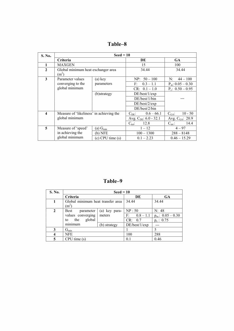
The summary of the results from the preceding discussions, for the selected seed value of 10 is listed in Table-8.

Table-8

The performance of DE and GA can be compared from this table with respect to the various criteria identified and defined. Out of the entire range of key parameter combinations considered, the range of the individual key parameter values converging to the global minimum heat exchanger area of 34.44 m2, along with the best strategies recommended are listed for DE and GA. For comparison of DE and GA, the characteristic criteria identified are the �likeliness� and the �speed� in achieving the global minimum. As a measure of �likeliness� the following parameters are defined: CDE and average CDE for DE; CGA and average CGA for GA; Ctot for both GA and DE. Similarly, as a measure of �speed� the parameters defined are: Gmin; NFE; and CPU time. From the range of the values of these identified parameters for the above criteria listed in Table-8, it is evident that DE has shown remarkable performance within 15 generations itself from both �likeliness� and �speed� point of view, which GA could not show even in 100 generations. Hence, it can be concluded that DE is significantly faster at optimization and has more likeliness in achieving the global optimum. The results shown in this comprehensive table, consolidate all the observations made and the conclusions drawn from the preceding discussions. So, the authors recommend the above range of the key parameter values (as listed in Table-8) for the optimal design of a shell-and-tube heat exchanger using differential evolution.

The performance of DE and GA is compared for the present problem in Table-9, with respect to the �best� parameters � parameter values converging to the global minimum out of the entire range considered.

Table-9

For NP=50, with DE/best/1/exp strategy, CR=0.7 and F = 0.8 to 1.1 (any value in steps of 0.1), as already been mentioned DE took one generation, 100 function evaluations and 0.1 seconds of CPU time. But with GA, for N = 48, pc = 0.75 and pm = 0.05 to 0.3 (any value in steps of 0.05) it took 5 generations, 288 function evaluations and 0.46 seconds of CPU time.

From Table-9, it can be seen that DE is almost 4.6 times faster than GA. And by using DE, there is 78.3 % savings in the computational time compared to GA. Comparing the results of the proprietary program (HTFS, STEP5) with these algorithms (both DE and GA), there is 37.4 % saving in the heat transfer area for

the case study considered. For the optimal shell-and-tube HED problem considered, the best population size using both DE and GA is seen to be around 7 times the number of design variables with about 70 percent crossover probability. Hence, for the heat duty of the case study taken up, the best design configuration of the shell-and-tube heat exchanger with respect to the design variables considered, corresponds to the global minimum heat exchanger area of 34.44 m2. The best design variables are listed in Table-10 along with the best key parameters of the DE algorithm used for this optimization.

Table-10

5. Conclusions

This paper demonstrates the first successful application of Differential Evolution for the optimal design of shell-and-tube heat exchangers. A generalized procedure has been developed to run the DE algorithm coupled with a function that uses Bell�s method of heat exchanger design, to find the global minimum heat exchanger area. For the case study taken up, application of all the ten different working strategies of DE are explored. The performance of DE and GA is compared. From this study we conclude that: 1. The population-based algorithms such as GAs and DE provide significant improvement in the optimal

designs, by achieving the global optimum, compared to the traditional designs. 2. For the present optimal shell-and-tube HED problem:

• The best population size, using both DE and GA, is about 7 times the number of design variables, • From �more likeliness� as well as �speed� point of view, DE/best/... strategies are better than

DE/rand/... for the selected seed value of 10, • DE/best/1/.. strategy is found to be the best out of the presently available ten strategies of DE.

3. Differential Evolution, a simple evolution strategy is significantly faster compared to GA. 4. DE achieves the global minimum over a wide range of its key parameters � indicating the �likeliness� of

achieving the true global optimum. 5. And DE proves to be a potential source for accurate and faster optimization.

Nomenclature

Ao - heat transfer area based on outer surface, m2 A(X) - objective function heat transfer area, m2 CDE - percentage of the combinations converging to the global mini-

-mum of 34.44 m2 of heat exchanger area, out of the 121 comb- -inations of F and CR considered (Tables-2 & 5)

CGA - percentage of the combinations converging to the global mini- -mum of 34.44 m2 of heat exchanger area, out of the 60 comb- -inations of pc and pm considered (Tables-7 & 9)

Cp - heat capacity at constant pressure, J/kg K CPU time - the time taken on 266MHz Pentium-II processor CR - crossover constant Ctot - percentage of the key parameter combinations converging to

the global minimum, out of the total number of combina- tions considered

C(X) - objective function heat exchanger cost D - number of design variables or dimension of the parameter vector F - weight applied to the random differential Ft - LMTD correction factor Gmin - minimum number of generations required to converge to the global minimum

k - thermal conductivity, W/m K N - population size in GA NP - population size in DE pc - crossover probability in GA pm - mutation probability in DE Q - heat duty, W r - random number ∆Tlm - log-mean temperature difference ∆Tm - mean temperature difference Uo.ass - assumed value of overall heat transfer coefficient based on

outside area, W/m2 0C U0,cal - calculated value of overall heat transfer coefficient based on

outside area, W/m2 0C x - a design variable X - a design configuration

Greek Symbols

ρ - density, kg/m3 µ - viscosity, kg/m s

Abbreviations

DE - Differential Evolution GA - Genetic Algorithms HE - Heat Exchanger HED - Heat Exchanger Design HTFS - Heat Transfer Flow Systems HTRI - Heat Transfer Research Institute LMTD - Log-Mean Temperature Difference MAXGEN - Maximum Number of Generations specified NFE - Number of Function Evaluations SA - Simulated Annealing

References

Allwright, J. R. A. & Carpenter, D. B. (1989). A distributed implementation of simulated annealing for the traveling salesman problem. Parall. Comput., 10, 335-338.

Androulakis, I. P. & Venkatasubramanian, V. (1991). A genetic algorithm framework for process design and optimization. Comput. Chem. Engng., 15(4), 217-228.

Athier, G., Floquet, P., Pibouleau, L., & Domenech, S. (1997a). Process optimization by simulated annealing and NLP procedures. Application to heat exchanger network synthesis. Comput. Chem. Engng., 21, S475-S480.

Athier, G., Floquet, P., Pibouleau, L., & Domenech, S. (1997b). Synthesis of heat exchanger network by simulated annealing and NLP procedures. A.I.Ch.E. J.,43(11), 3007-3020.

Babu, B. V. & Munawar, S. A. (2000). Differential Evolution for the optimal design of heat exchangers, Proceedings of All-India seminar on Chemical Engineering Progress on Resource Development: A Vision 2010 and Beyond, IE (I), Bhubaneswar, India, March 11, 2000.

Babu, B. V. & Sastry, K. K. N. (1999). Estimation of heat transfer parameters in a trickle-bed reactor using differential evolution and orthogonal collocation, Comp. Chem. Engng., 23, 327 - 339.

Babu, B. V. & Vivek, N. (1999). Genetic algorithms for estimating heat transfer parameters in trickle bed reactors, Proceedings of 52nd Annual session of IIChE (CHEMCON-99), Chandigarh, India, December 20 � 23, 1999.

Cerny, V. (1985). Thermodynamical approach to the traveling salesman problem: An efficient simulation algorithm. J. Opim. Theo. Appl., 45, 41-51.

Chaudhuri, P. D., Urmila, M. D. & Jefery, S.L. (1997). An automated approach for the optimal design of heat exchangers, Ind. Engng. Chem. Res., 36, 3685 - 3693.

Chiou, J. P. & Wang, F. S. (1999). Hybrid method of evolutionary algorithms for static and dynamic optimization problems with application to a fed-batch fermentation process. Comput. Chem. Engng., 23(9), 1277-1291.

Cordero, J. C., Davin, A., Floquet, P., Pibouleau, L., & Domenech, S. (1997). Synthesis of optimal reactor networks using mathematical programming and simulated annealing. Comput. Chem. Engng., 21, S47-S52.

Das, H., Cummings, P. T., & Levan, M. D. (1990). Scheduling of serial multiproduct batch processes via simulated annealing. Comput. Chem. Engng., 14(12), 1351-1362.

Davis, L. (1991). Handbook of genetic algorithms. Newyork: Van Nostrand Reinhold.

Deb, K. (1996). Optimization for engineering design: Algorithms and examples, New Delhi: Prentice-Hall.

Dolan, W. V., Cummings, P. T., & Levan, M. D. (1990). Algorithmic efficiency of simulated annealing for heat exchanger networks. Comput. Chem. Engng., 14(10), 1039-1050.

Floquet, P., Pibouleau, L., & Domenech, S. (1994). Separation sequence synthesis: How to use simulated annealing procedure?. Comput. Chem. Engng., 18(11/12), 1141-1148.

Fraga, E. S. & Senos Matias, T. R. (1996). Synthesis and optimization of a nonideal distillation system using a parallel genetic algorithm. Comput. Chem. Engng., 20, S79-S84.

Goldberg, D. E. (1989). Genetic algorithms in search, optimization, and machine learning, Reading, MA: Addison-Wesley.

Joshi, R. & Sanderson, A. C. (1999). Minimal representation multisensor fusion using differential evolution. IEEE Transcations on Systems, Man and Cybernetics, Part A 29(1), 63-76.

Kirkpatrik, S., Gelatt, C. D. & Vechhi, M. P. (1983). Optimization by simulated annealing, Science, 220(4568), 671-680.

Lee, M. H., Han, C., & Chang, K. S. (1999). Dynamic optimization of a continuous polymer reactor using a modified differential evolution. Ind. Engng. Chem. Res., 38(12), 4825-4831.

Maia, L. O. A., Vidal de Carvalho, L. A., & Qassim, R. Y. (1995). Synthesis of utility systems by simulated annealing. Comput. Chem. Engng., 19(4), 481-488.

Manish, C. T., Yan Fu & Urmila, M. D. (1999). Optimal design of heat exchangers: A genetic algorithm framework, Ind. Engng. Chem. Res., 38, 456- 467.

Masters, T. & Land, W. (1997). A new training algorithm for the general regression neural network. 1997 IEEE International conference on Systems, Man and Cybernetics, Computational cybernetics and Simulation, 3, 1990-1994.

McLeod, A. S., Johnston, M. E., & Gladden, L. F. (1997). Development of a genetic algorithm for molecular scale catalyst design. J. Catal., 167, 279-285.

Moriyama, H. & Shimizu, K. (1996). On-line optimization of culture temperature for ethanol fermentation using a genetic algorithm. J. Chem. Technol. Biotechnol., 66, 217-222.

Moros, R., Kalies, H., Rex, H. G., & Schaffarczyk. St. (1996). A genetic algorithm for generating initial parameter estimations for kinetic models of catalytic processes. Comput. Chem. Engng., 20, 1257-1270.

Patel, A. N., Mah, R. S. H., & Karimi, I. A. (1991). Preliminary design of multiproduct noncontinuous plants using simulated annealing. Comput. Chem. Engng., 15(7), 451-469.

Perry, R. H. & Green, D. (1993). Perry�s chemical engineers� handbook, 6th ed., New York: McGHI Editions, Chem. Engng. Series.

Price, K. & Storn, R. (1997). Differential evolution, Dr. Dobb�s J., 18-24.

Price, K. & Storn, R. (2000). Web site of Price and Storn as on April, 2000. http://www.ICSI.Berkeley.edu/~storn/code.html

Rutenbar, R. A. (1989). Simulated annealing algorithms: An overview, IEEE Circuits Devices Magazine, 100, 19-26.

Sastry, K. K. N., Behra, L., & Nagrath, I. J. (1998). Differential evolution based fuzzy logic controller for nonlinear process control. Fundamenta Informaticae: Special Issue on Soft Comput.

Sinnott, R. K. (1993). Coulson & Richardson�s Chemical Engineering (Design), 6, 2nd ed., Newyork: Pergamon.

Stair, C. & Fraga, E. S. (1995). Optimization of unit operating conditions for heat integrated processes using genetic algorithms. Proc. 1995. Inst. Chem. Engng. Research Event, Inst. Chem. Engrs., 95-97.

Storn, R. (1995). Differential evolution design of an IIR-filter with requirements for magnitude and group delay. TR-95-018, ICSI.

Upreti, S. R. & Deb, K. (1996). Optimal design of an ammonia synthesis reactor using genetic algorithms. Comput. Chem. Engng., 21, 87-93.

Venkatasubramanian, V., Chan, K., & Caruthers, J. M. (1994). Computer-aided molecular design using genetic algorithms. Comput. Chem. Engng., 18, 833-844.

Wang, F. S., Jing, C. H., & Tsao, G. T. (1998). Fuzzy-decision-making problems of fuel ethanol production, using a genetically engineered yeast. Ind. Engng. Chem. Res., 37(8), 3434-3443.

Wang, F. S. & Cheng, W. M. (1999). Simultaneous optimization of feeding rate and operation parameters for fed-batch fermentation processes. Biotechnol. Prog., 15(5), 949-952.

Wolf, D. & Moros, R. (1997). Estimating rate constants of heterogeneous catalytic reactions without supposition of rate determining surface steps- An application of genetic algorithm. Chem. Engng. Sci., 52, 1189-1199.

List of Tables

Table-1 Problem formulation for the optimal design of a shell-and-tube heat exchanger Table-2 Effect of seed on DE strategies w.r.t. CDE Table-3 Effect of seed on DE strategies w.r.t. Gmin Table-4 Effect of seed on DE strategies w.r.t. number of combinations of F and CR Table-5 Effect of NP on DE strategies w.r.t. CDE

Table-6 Effect of NP on DE strategies w.r.t. Gmin Table-7 GA parameters converging to the global minimum Table-8 Comparison of DE and GA w.r.t. various criteria for the entire range of parameters Table-9 Comparison of DE and GA w.r.t. various criteria for the best

parameters Table-10 Summary of the proposed final design for the case study

List of Figures

Fig. 1 Design algorithm for shell-and-tube heat exchangers Fig. 2 Comparison of DE strategies for best vector perturbation with F as a parameter [ (a) F=0.5; (b) F=0.6 ] Fig. 3 Comparison of DE strategies for best vector perturbation with F as a parameter [ (a) F=0.7; (b) F=0.8 ] Fig. 4 Comparison of DE strategies for best vector perturbation with F as a parameter [ (a) F=0.9; (b) F=1.0 ] Fig. 5 Comparison of DE strategies for random vector perturbation with F as a

parameter [ (a) F=0.7; (b) F=0.8 ] Fig. 6 Comparison of DE strategies for random vector perturbation with F as a

parameter [ (a) F=0.9; (b) F=1.0 ] Fig. 7 Comparison of DE strategies for random vector perturbation with CR as a

parameter [ (a) CR=0; (b) CR=0.3 ] Fig. 8 Comparison of DE strategies for random vector perturbation with CR as a

parameter [ (a) CR=0.5; (b) CR=0.7 ] Fig. 9 Comparison of DE strategies for random vector perturbation with CR as a

parameter [ (a) CR=0.9; (b) CR=1.0 ]

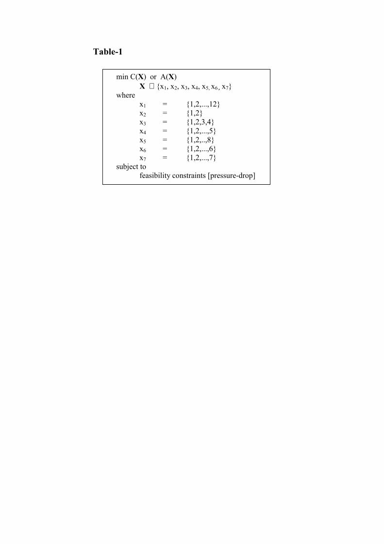
Table-1

min C(X) or A(X) X ∈ {x1, x2, x3, x4, x5, x6 ̧x7}

where x1 = {1,2,...,12} x2 = {1,2} x3 = {1,2,3,4} x4 = {1,2,...,5} x5 = {1,2,..,8} x6 = {1,2,...,6} x7 = {1,2,...,7}

subject to feasibility constraints [pressure-drop]

Table-2

NP = 70 & MAXGEN = 30

S. No. Strategy Seed = 3

CDE

Seed = 5

CDE

Seed = 7

CDE

Seed = 10

CDE

Seed = 15

CDE

Seed = 20

CDE

Average of CDE w.r.t. seed

1 DE/best/1/exp

41.3 62.0 52.1 48.0 57.0 45.5 51.0

2 DE/rand/1/exp

36.4 72.0 68.6 51.2 61.1 39.7 54.8

3 DE/rand-to-best/1/exp

44.6 53.0 46.3 43.0 48.8 43.0 46.5

4 DE/best/2/exp

44.6 72.7 72.0 66.1 53.7 47.1 59.4

5 DE/rand/2/exp

28.1 72.0 53.7 48.8 46.3 43.0 48.7

6 DE/best/1/bin

37.2 57.0 44.6 68.6 47.1 47.9 50.4

7 DE/rand/1/bin

44.6 81.8 59.5 37.2 60.0 38.8 53.7

8 DE/rand-to-best/1/bin

37.2 48.0 42.1 63.6 38.8 35.5 44.2

9 DE/best/2/bin

48.8 61.2 57.0 64.5 52.1 58.7 57.1

10 DE/rand/2/bin 43.8 68.6 48.0 55.4 39.7 68.6 54.0 Average of CDE

w.r.t. strategies 40.7 64.8 54.4 54.6 50.5 46.8

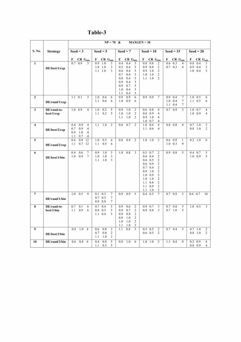
Table-3

NP = 70 & MAXGEN = 30

S. No. Strategy Seed = 3

F CR Gmin

Seed = 5

F CR Gmin

Seed = 7

F CR Gmin

Seed = 10

F CR Gmin

Seed = 15

F CR Gmin

Seed = 20

F CR Gmin 1

DE/best/1/exp

0.7 0.9 3 0.9 1.0 3 1.0 1.0 3 1.1 1.0 3

0.4 0.4 5 0.5 0.4 5 0.6 0.4 5 0.7 0.4 5 0.8 0.4 5 0.9 0.4 5 0.9 0.7 5 1.0 0.4 5 1.1 0.4 5

0.8 0.8 2 0.9 0.8 2 0.9 1.0 2 1.0 1.0 2 1.1 1.0 2

0.6 0.3 4 0.7 0.3 4

0.8 0.4 3 0.9 0.4 3 1.0 0.4 3

2

DE/rand/1/exp

1.1 0.1 3 1.0 0.6 6 1.1 0.6 6

0.9 0.9 6 1.0 0.9 6

0.9 0.9 7 0.9 0.4 7 1.0 0.4 7 1.1 0.4 7

1.0 0.5 6 1.1 0.5 6

3 DE/rand-to-best/1/exp

1.0 0.9 4 1.0 0.2 5 1.1 0.2 5

0.9 1.0 2 1.0 1.0 2 1.1 1.0 2

0.6 0.8 4 0.8 0.9 4 0.9 1.0 4 1.0 0.7 4

0.7 0.9 3

1.0 0.7 4 1.0 0.9 4

4

DE/best/2/exp

0.4 0.9 4 0.7 0.9 4 0.9 1.0 4 1.1 0.7 4

1.1 1.0 2 0.8 0.7 2 1.0 0.6 4 1.1 0.6 4

0.8 0.8 4 0.7 1.0 2 0.8 1.0 2

5

DE/rand/2/exp

0.6 0.9 12 1.1 0.7 12

1.0 0.5 6 1.1 0.5 6

0.8 0.9 2 1.0 1.0 3 0.6 0.9 1 1.0 0.3 9

0.2 1.0 6

6

DE/best/1/bin

0.4 0.6 7 1.0 0.9 7

0.9 1.0 3 1.0 1.0 3 1.1 1.0 3

1.0 0.8 3 0.5 0.7 2 0.6 0.4 2 0.6 0.5 2 0.6 0.9 2 0.7 0.4 2 0.9 1.0 2 1.0 0.9 2 1.0 1.0 2 1.1 0.8 2 1.1 0.9 2 1.1 1.0 2

0.9 0.8 5 0.4 0.7 5 1.0 0.9 5

7

DE/rand/1/bin

1.0 0.5 9 0.1 0.3 7 0.7 0.5 7 0.8 0.8 7

0.9 0.9 5 0.4 0.5 7 0.7 0.9 3 0.6 0.7 10

8 DE/rand-to-best/1/bin

0.7 0.1 6 1.1 0.9 6

0.7 0.4 5 0.8 0.5 5 1.1 0.4 5

0.9 0.6 2 0.9 0.7 2 0.9 0.8 2 0.9 1.0 2 1.0 1.0 2 1.1 1.0 2

0.9 0.7 3 0.9 0.8 3

0.7 0.8 5 0.7 1.0 5

1.0 0.5 3

9

DE/best/2/bin

0.9 1.0 4 0.6 0.8 2 0.7 0.8 2 1.1 1.0 2

1.1 0.8 3 0.5 0.5 2 0.6 0.5 2

0.7 0.4 5 0.7 1.0 2 0.8 1.0 2

10 DE/rand/2/bin 0.6 0.8 6 0.4 0.8 5 1.1 0.5 5

0.9 1.0 6 1.0 1.0 3 1.1 0.4 9 0.2 0.9 4 0.8 0.9 4

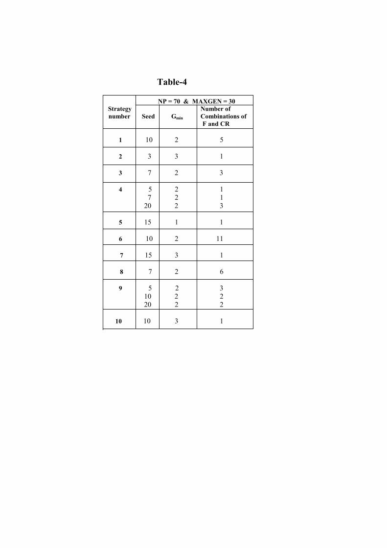
Table-4

NP = 70 & MAXGEN = 30 Strategy Number of number Seed Gmin Combinations of F and CR 1 10 2 5 2 3 3 1 3 7 2 3 4 5 2 1

7 2 1 20 2 3 5 15 1 1 6 10 2 11 7 15 3 1 8 7 2 6 9 5 2 3 10 2 2 20 2 2 10 10 3 1

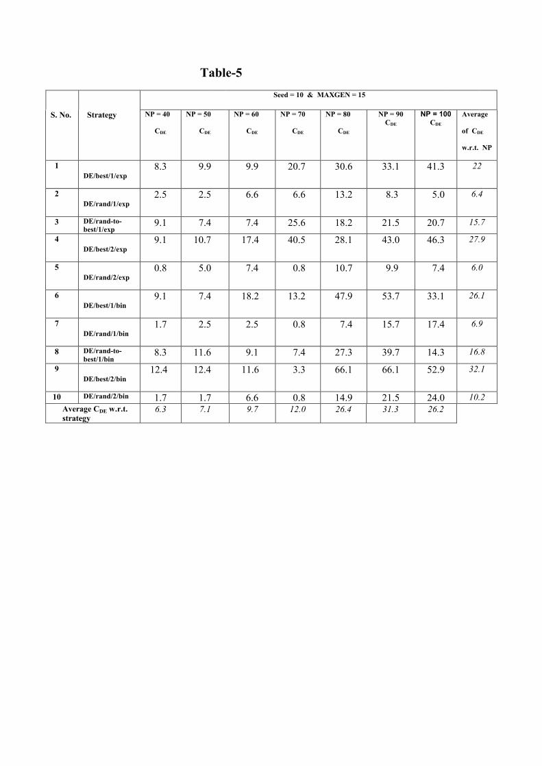
Table-5

Seed = 10 & MAXGEN = 15

S. No. Strategy NP = 40

CDE

NP = 50

CDE

NP = 60

CDE

NP = 70

CDE

NP = 80

CDE

NP = 90 CDE

NP = 100 CDE

Average

of CDE

w.r.t. NP

1 DE/best/1/exp

8.3 9.9 9.9 20.7 30.6 33.1 41.3 22

2 DE/rand/1/exp

2.5 2.5 6.6 6.6 13.2 8.3 5.0 6.4

3 DE/rand-to-best/1/exp

9.1 7.4 7.4 25.6 18.2 21.5 20.7 15.7

4 DE/best/2/exp

9.1 10.7 17.4 40.5 28.1 43.0 46.3 27.9

5 DE/rand/2/exp

0.8 5.0 7.4 0.8 10.7 9.9 7.4 6.0

6 DE/best/1/bin

9.1 7.4 18.2 13.2 47.9 53.7 33.1 26.1

7 DE/rand/1/bin

1.7 2.5 2.5 0.8 7.4 15.7 17.4 6.9

8 DE/rand-to-best/1/bin

8.3 11.6 9.1 7.4 27.3 39.7 14.3 16.8

9 DE/best/2/bin

12.4 12.4 11.6 3.3 66.1 66.1 52.9 32.1

10 DE/rand/2/bin 1.7 1.7 6.6 0.8 14.9 21.5 24.0 10.2 Average CDE w.r.t.

strategy 6.3 7.1 9.7 12.0 26.4 31.3 26.2

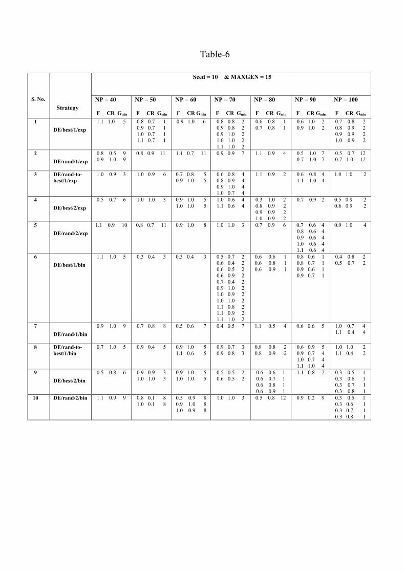
Table-6

Seed = 10 & MAXGEN = 15

S. No.

Strategy NP = 40

F CR Gmin

NP = 50

F CR Gmin

NP = 60

F CR Gmin

NP = 70

F CR Gmin

NP = 80

F CR Gmin

NP = 90

F CR Gmin

NP = 100

F CR Gmin 1

DE/best/1/exp

1.1 1.0 5 0.8 0.7 1 0.9 0.7 1 1.0 0.7 1 1.1 0.7 1

0.9 1.0 6 0.8 0.8 2 0.9 0.8 2 0.9 1.0 2 1.0 1.0 2 1.1 1.0 2

0.6 0.8 1 0.7 0.8 1

0.6 1.0 2 0.9 1.0 2

0.7 0.8 2 0.8 0.9 2 0.9 0.9 2 1.0 0.9 2

2

DE/rand/1/exp

0.8 0.5 9 0.9 1.0 9

0.8 0.9 11 1.1 0.7 11 0.9 0.9 7 1.1 0.9 4 0.5 1.0 7 0.7 1.0 7

0.5 0.7 12 0.7 1.0 12

3 DE/rand-to-best/1/exp

1.0 0.9 3 1.0 0.9 6 0.7 0.8 5 0.9 1.0 5

0.6 0.8 4 0.8 0.9 4 0.9 1.0 4 1.0 0.7 4

1.1 0.9 2 0.6 0.8 4 1.1 1.0 4

1.0 1.0 2

4

DE/best/2/exp

0.5 0.7 6 1.0 1.0 3 0.9 1.0 5 1.0 1.0 5

1.0 0.6 4 1.1 0.6 4

0.3 1.0 2 0.8 0.9 2 0.9 0.9 2 1.0 0.9 2

0.7 0.9 2 0.5 0.9 2 0.6 0.9 2

5

DE/rand/2/exp

1.1 0.9 10 0.8 0.7 11 0.9 1.0 8 1.0 1.0 3 0.7 0.9 6 0.7 0.6 4 0.8 0.6 4 0.9 0.6 4 1.0 0.6 4 1.1 0.6 4

0.9 1.0 4

6

DE/best/1/bin

1.1 1.0 5 0.3 0.4 3 0.3 0.4 3 0.5 0.7 2 0.6 0.4 2 0.6 0.5 2 0.6 0.9 2 0.7 0.4 2 0.9 1.0 2 1.0 0.9 2 1.0 1.0 2 1.1 0.8 2 1.1 0.9 2 1.1 1.0 2

0.6 0.6 1 0.6 0.8 1 0.6 0.9 1

0.8 0.6 1 0.8 0.7 1 0.9 0.6 1 0.9 0.7 1

0.4 0.8 2 0.5 0.7 2

7

DE/rand/1/bin

0.9 1.0 9 0.7 0.8 8 0.5 0.6 7 0.4 0.5 7 1.1 0.5 4 0.6 0.6 5 1.0 0.7 4 1.1 0.4 4

8 DE/rand-to-best/1/bin

0.7 1.0 5 0.9 0.4 5 0.9 1.0 5 1.1 0.6 5

0.9 0.7 3 0.9 0.8 3

0.8 0.8 2 0.8 0.9 2

0.6 0.9 5 0.9 0.7 4 1.0 0.7 4 1.1 1.0 4

1.0 1.0 2 1.1 0.4 2

9

DE/best/2/bin

0.5 0.8 6 0.9 0.9 3 1.0 1.0 3

0.9 1.0 5 1.0 1.0 5

0.5 0.5 2 0.6 0.5 2

0.6 0.6 1 0.6 0.7 1 0.6 0.8 1 0.6 0.9 1

1.1 0.8 2 0.3 0.5 1 0.3 0.6 1 0.3 0.7 1 0.3 0.8 1

10 DE/rand/2/bin 1.1 0.9 9 0.8 0.1 8 1.0 0.1 8

0.5 0.9 8 0.9 1.0 8 1.0 0.9 8

1.0 1.0 3 0.5 0.8 12 0.9 0.2 9 0.3 0.5 1 0.3 0.6 1 0.3 0.7 1 0.3 0.8 1

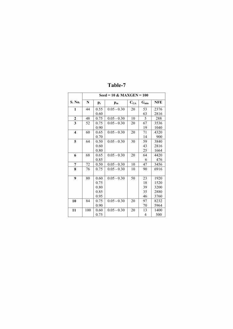
Table-7

Seed = 10 & MAXGEN = 100

S. No. N pc pm CGA Gmin NFE

1 44

0.55 0.60

0.05 - 0.30 20

53 63

2376 2816

2 48 0.75 0.05 - 0.30 10 5 288 3 52 0.75

0.90 0.05 - 0.30 20 67

19 3536 1040

4 60 0.65 0.70

0.05 - 0.30 20 71 14

4320 900

5 64 0.50 0.60 0.80

0.05 - 0.30 30 59 43 25

3840 2816 1664

6 68 0.65 0.85

0.05 - 0.30 20 64 6

4420 476

7 72 0.50 0.05 - 0.30 10 47 3456 8 76 0.75 0.05 - 0.30 10 90 6916

9 80 0.60

0.75 0.80 0.85 0.95

0.05 - 0.30 50 23 18 39 35 46

1920 1520 3200 2880 3760

10 84 0.75 0.90

0.05 - 0.30 20 97 70

8232 5964

11 100 0.60 0.75

0.05 - 0.30 20 13 4

1400 500

Table�8

Seed = 10 S. No. Criteria DE GA

1 MAXGEN 15 100 2 Global minimum heat exchanger area

(m2) 34.44 34.44

NP: 50 � 100 N: 44 � 100 F: 0.3 � 1.1 Pm: 0.05 � 0.30

(a) key parameters

CR: 0.1 � 1.0 Pc: 0.50 � 0.95 DE/best/1/exp DE/best/1/bin DE/best/2/exp

3 Parameter values converging to the global minimum

(b)strategy

DE/best/2/bin

---

CDE: 0.6 � 66.1 CGA: 10 - 50 Avg. CDE: 6.0 - 32.1 Avg. CGA: 20.9

4 Measure of �likeliness� in achieving the global minimum

Ctot: 12.8 Ctot : 14.4 (a) Gmin 1 � 12 4 � 97 (b) NFE 100 � 1300 288 � 8148

5 Measure of �speed� in achieving the global minimum (c) CPU time (s) 0.1 � 2.23 0.46 � 15.29

Table�9

Seed = 10 S. No. Criteria DE GA

1 Global minimum heat transfer area (m2)

34.44 34.44

NP : 50 N: 48 F: 0.8 � 1.1 pm : 0.05 � 0.30

(a) key para-meters

CR: 0.7 pc : 0.75

2 Best parameter values converging to the global minimum (b) strategy DE/best/1/exp ---

3 Gmin 1 5 4 NFE 100 288 5 CPU time (s) 0.1 0.46

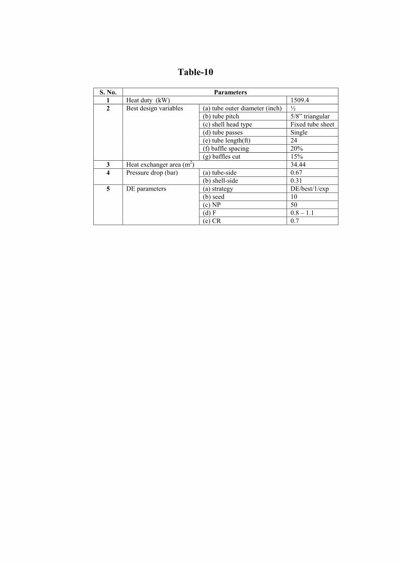
Table-10

S. No. Parameters 1 Heat duty (kW) 1509.4

(a) tube outer diameter (inch) ½ (b) tube pitch 5/8� triangular (c) shell head type Fixed tube sheet (d) tube passes Single (e) tube length(ft) 24 (f) baffle spacing 20%

2 Best design variables

(g) baffles cut 15% 3 Heat exchanger area (m2) 34.44

(a) tube-side 0.67 4 Pressure drop (bar) (b) shell-side 0.31 (a) strategy DE/best/1/exp (b) seed 10 (c) NP 50 (d) F 0.8 � 1.1

5 DE parameters

(e) CR 0.7