Optimal design of a CO2 capture unit with

assessment of solvent degradation

Grégoire Léonard

Mai 2013

Thèse présentée en vue de l’obtention du grade de

Docteur en Sciences de l’Ingénieur

II

III

Summary

In response to increasing environmental concerns and globally growing energy demand, CO2

capture, re-use and storage technologies have been proposed to reduce the emissions of

carbon dioxide resulting from fossil fuel combustion. In the present thesis, the post-

combustion CO2 capture with amine solvents is studied for the case of fossil fuel-fired power

plants. This end-of-pipe technology treats the flue gas after the combustion so that operating

power plants can be retrofitted to rapidly reduce their CO2 emissions. However, different

drawbacks still limit the development of this technology. At the operational level, the two

main drawbacks are the high energy requirement for desorbing CO2 (leading to a decrease by

about 30% of the plant efficiency) and the environmental impact related to the emissions of

amine solvent and its degradation products to the atmosphere. The main originality of the

present work is to simultaneously consider both aspects within a global model of the CO2

capture process assessing solvent degradation. This study has been performed in two phases.

In the first phase, experimental data about oxidative and thermal degradation of the solvent

have been gained by using newly-developed test benches. The influence of process operating

parameters on solvent degradation and on the formation of degradation products has been

quantified by appropriate analytical techniques. It results from this study that the main

mechanism of solvent degradation is the oxidative degradation. This is the case in laboratory

conditions as well as in industrial CO2 capture pilots for which degraded solvent samples

could be obtained. Lab experiments show that this type of degradation is enhanced when the

O2 concentration in the flue gas, the gas-liquid contact or the temperature are increased.

Moreover, it appears that the presence of dissolved metals in the solvent catalyzes the

oxidative degradation. On the contrary, the presence of CO2 reduces the rate of oxidative

degradation. Adding degradation inhibitors also reduces the oxidative degradation, more or

less successfully depending on the tested inhibitor. Regarding thermal degradation, significant

degradation is only observed in the presence of CO2 and at a high temperature (140°C).

Thermal degradation is not influenced by the presence of dissolved metals, but some

degradation inhibitors have a negative influence on the solvent thermal stability.

The second phase has consisted in developing a model of the CO2 capture process using the

Aspen Plus software package. This kind of model allows the evaluation of the process energy

requirement. The main innovation of this thesis was to propose kinetics parameters for the

oxidative and the thermal degradations based on the results of the experimental study, and to

include this kinetics into the process model. This model has led to the identification of

oxidative degradation in the absorber as the major cause of solvent loss in the process, which

is in agreement with results reported in CO2 capture pilot plants. The emission of ammonia

(main oxidative degradation product of the amine solvent) has also been confirmed to be one

of the main environmental issues of the CO2 capture process. Furthermore, the resulting

model is used to evaluate the influence of operating conditions both on the process energy

requirement and on its environmental impact. The largest energy savings are observed when

increasing the stripper pressure and the solvent concentration, while the most significant

increases of the solvent consumption are due to the increased oxygen concentration in the flue

gas and to the higher solvent concentration. Two process improvements have also been tested

(absorber intercooling and lean vapor compression), leading to a significant decrease of the

total process energy requirement with low influence on solvent degradation. Thanks to this

model, optimum operating conditions have been proposed for CO2 capture, reducing the

process energy requirement by 12% at equivalent solvent consumption rate.

IV

However, the solvent consumption rate is under-predicted by the model in comparison to pilot

plant studies. Thus, different perspectives are proposed to improve the model, among others

by considering the effect of dissolved metals and flue gas contaminants like SOx and NOx in

the degradation kinetics. Moreover, this methodology has been developed for an aqueous

solution of monoethanolamine (MEA), which is the benchmark solvent for CO2 capture.

Alternative promising solvents may be considered following the same methodology to further

improve the CO2 capture process.

Finally, this kind of model could and should be used for the design of CO2 capture plants to

consider not only the process energy penalty, but also its environmental penalty which is

particularly relevant for large-scale applications.

V

Résumé

En réponse à la prise de conscience des problématiques environnementales et à la demande

croissante en énergie, les techniques de capture, utilisation et stockage du CO2 ont été

proposées pour réduire les émissions de CO2 résultant de la combustion de ressources fossiles.

Dans cette thèse, la capture post-combustion du CO2 au moyen de solvants aminés a été

étudiée pour le cas des centrales électriques au charbon et au gaz naturel. Cette technologie

traite les gaz de combustion, permettant ainsi d’équiper des centrales existantes afin de

rapidement diminuer leurs émissions de CO2. Cependant, différents freins limitent encore le

développement de cette technique. Au niveau opératoire, les deux principaux désavantages

sont un besoin énergétique élevé pour la désorption du CO2 (entraînant une diminution de

près de 30% du rendement de la centrale) et un impact environnemental lié aux émissions du

solvant aminé et de ses produits de dégradation dans l’atmosphère. La principale originalité

de ce travail est de considérer simultanément ces deux aspects au sein d’un modèle global du

procédé de capture du CO2 incluant la dégradation des solvants. Cette étude a été menée en

deux étapes.

Dans la première étape, des données expérimentales sur la dégradation oxydative et thermique

des solvants ont été obtenues sur des bancs d’essais développés dans le cadre de cette thèse.

L’influence des paramètres opératoires sur la dégradation des solvants et sur la formation de

produits de dégradation a été quantifiée par des techniques analytiques appropriées. Il ressort

de cette étude que le principal mécanisme de dégradation des solvants est la dégradation

oxydative, que ce soit dans les conditions du laboratoire ou dans des pilotes industriels de

capture du CO2 pour lesquels des échantillons de solvant dégradés ont pu être obtenus. Les

tests en laboratoire montrent que ce type de dégradation est accéléré lorsque la teneur en O2

des gaz de combustion, le contact gaz-liquide ou la température sont augmentés. De plus, il

apparaît que la présence de métaux dissous dans le solvant catalyse la dégradation oxydative.

Au contraire, la présence de CO2 diminue le taux de dégradation oxydative. L’ajout

d’inhibiteurs de dégradation oxydative diminue également ce type de dégradation avec plus

ou moins de succès selon l’inhibiteur testé. En ce qui concerne la dégradation thermique, elle

n’intervient de façon significative qu’en présence de CO2 et à haute température (140°C). Elle

n’est pas influencée par la présence de métaux, mais certains inhibiteurs de dégradation

oxydative ont une influence négative sur la stabilité thermique du solvant.

La seconde étape a consisté à développer un modèle du procédé de capture du CO2 au moyen

du logiciel de simulation Aspen Plus. Ce type de modèle permet d’évaluer le besoin

énergétique du procédé. La principale innovation de cette thèse a été de proposer une

cinétique de dégradation oxydative et thermique du solvant sur base des résultats de l’étude

expérimentale, et d’inclure cette cinétique dans le modèle du procédé. La dégradation

oxydative du solvant se produisant dans l’absorbeur a été identifiée comme la principale

contribution à la consommation de solvant, confirmant les résultats observés dans des

installations pilotes de capture du CO2. Il est également montré que l’émission d’ammoniac

(principal produit de la dégradation oxydative du solvant aminé) constitue un des plus grands

défis environnementaux du procédé de capture. De plus, le modèle résultant a permis

d’évaluer l’influence des conditions opératoires à la fois sur le besoin énergétique du procédé

et sur son impact environnemental. Les réductions les plus importantes des besoins

énergétiques du procédé ont été obtenues en augmentant la pression de régénération et la

concentration du solvant. Les augmentations les plus prononcées de la consommation de

solvant sont dues à l’augmentation de la concentration en oxygène dans les gaz de fumée et à

l’augmentation de la concentration de solvant. Deux modifications de procédé ont également

VI

été étudiées (refroidissement intermédiaire dans l’absorbeur et compression de vapeur

pauvre), réduisant significativement le besoin énergétique du procédé tout en montrant peu

d’influence sur la consommation de solvant. Grâce à ce modèle, des conditions opératoires

optimales ont été proposées, permettant de réduire le besoin énergétique du procédé de 12% à

consommation de solvant égale.

Cependant, le modèle sous-estime la consommation de solvant observée dans les installations

pilotes. En conséquence, différentes pistes d’amélioration sont proposées, considérant

notamment l’effet des métaux dissous et des impuretés présentes dans les gaz de combustion

(NOx et SOx) dans le modèle. De plus, cette méthodologie développée pour une solution

aqueuse de monoethanolamine (MEA, le solvant de référence pour la capture de CO2)

pourrait également être appliquée à d’autres solvants prometteurs pour la capture post-

combustion du CO2.

Finalement, ce type de modèle pourrait et devrait être utilisé lors du design d’installations de

capture du CO2 en vue de considérer non seulement l’impact énergétique de l’installation sur

la centrale, mais également son impact environnemental qui s’avère particulièrement

important dans le cas d’applications à grande échelle.

VII

Acknowledgements

First of all, I would like to sincerely thank Professor Georges Heyen for giving me the

opportunity to learn and to evolve as a member of the Laboratory for Analysis and Synthesis

of Chemical Systems. His advices have always been judicious and he was always available to

answer my questions, and I am very grateful for that.

I also thank Professor Dominique Toye for welcoming me in her team at the experimental hall

for applied chemistry. I am also very grateful for the constructive discussions that have

guided the realization of this work and improved its quality.

I also want to thank the other members of the thesis committee for their interest and

participation to the evaluation of this work: Professor Diane Thomas from the University of

Mons, Mrs Marie-Laure Thielens from Laborelec and Doctor Ludovic Raynal from the IFP

Energies Nouvelles, as well as Professor Pierre Dewallef, Professor Angélique Léonard and

Professor Michel Crine form the University of Liège.

I am very grateful to the Belgian FRIA-FNRS for the financial support of this PhD Thesis

during four years, giving me the opportunity to develop the present research project.

I also address a special thanks to the company Laborelec who partially funded this work and

provided technical support. I especially thank you Hélène Lepaumier, for the relevant advices

and the enthusiastic discussions about solvent degradation, Frédéric Mercier, Han Huynh,

Fabrice Blandina, and Philippe Demlenne for the nice collaboration and the enriching

exchanges.

Then, I also sincerely thank Ms Ségolène Belletante, student at the INP Ensiacet Toulouse,

Ms Marion Bascougnano, formerly student at the IUT Paul Cézanne Aix- Marseille, and Mr

Bruno Cabeza Mogador, formerly student at the University of Liège, for their participation to

this PhD thesis. Without their support, it would have been impossible to obtain all the

experimental and modeling results presented in this work. Their support and their motivation

in this research project have been considerably appreciated.

I also thank the PhD students met during the time of this work and that have contributed to its

achievement. I especially thank Lionel Dubois from the University of Mons for the

enthusiastic collaboration and the constant availability, as well as Alexander Voice from the

University of Texas at Austin, for the enriching discussions and the sending of inhibited

amine solvents that have been tested in this work.

Many thanks are addressed to the people of the Chemical Engineering Department that have

contributed to make this work possible by their helpful technical advices, and to the whole

department staff for the nice working atmosphere during this research project.

Finally, my last thanks go to my family, to my parents that have always supported and

encouraged my choices, and to Séverine for her patience and her love.

VIII

IX

Table of content

Summary III

Résumé V

Acknowledgements VII

Chapter I: Introduction

1. General context 3

2. Carbon capture and storage 5

2.1 Basic techniques for CO2 capture 5

2.2 CO2 capture processes 8

2.3 Transport, utilization and storage 13

3. Post-combustion capture with amine solvents 17

3.1 Process description 17

3.2 Main post-combustion capture projects 18

3.3 Advantages and drawbacks of post-combustion capture with amine solvents 20

4. Objectives 22

Chapter II: Experimental study of amine solvent degradation

1. Introduction 25

2. State of the art 27

2.1 Degradation mechanisms 27

2.2 Main studies published about MEA degradation 32

2.3 Influence of dissolved metals 37

2.4 Possible answers to amine degradation 39

3. Experimental methods 46

3.1 Semi-batch degradation test rig 46

3.2 Batch degradation cylinders 49

3.3 Analytical methods 49

4. Semi-batch experiments 62

4.1 Base case 62

X

4.2 Influence of the gas feed 63

4.3 Influence of the agitation rate 68

4.4 Influence of the test duration 72

4.5 Influence of the temperature 73

4.6 Influence of additives 77

4.7 Experimental error 82

5. Batch Experiments 85

5.1 Influence of CO2 85

5.2 Influence of temperature 87

5.3 Influence of degradation inhibitors 89

6. Conclusions 92

Chapter III: Simulation of the CO2 capture process

1. Introduction 95

2. State of the art 97

2.1 Thermodynamic model 97

2.2 Reactive absorption 101

2.3 Main modeling studies about CO2 capture with MEA 113

3. Model construction 128

3.1 Mobile Pilot Unit models 129

3.2 Esbjerg Pilot Plant models 133

4. Simulation results 143

4.1 Equilibrium and rate-based model comparison 143

4.2 Dynamic modeling 146

4.3 Degradation modeling 150

5. Conclusions 163

Chapter IV: Conclusions and perspectives

1. Conclusions 166

2. Perspectives 168

XI

Bibliography 170

Figure index 186

Table index 191

Abbreviation list 192

Appendices 194

Appendix 1: Influence of dissolved metals on MEA degradation 195

Appendix 2: Influence of degradation inhibitors for the MEA solvent 205

Appendix 3: Risk analysis for the Degradation Test Rig. 214

Appendix 4: Error analysis 225

Appendix 5: Experimental results 227

List of publications 238

Introduction

2

Chapter I

Introduction

“To believe with certainty, we must begin by doubting”

Polish quote

Introduction

3

1. General context

One of the biggest challenges our modern society has to face is the preservation of the

environment combined with a growing world energy demand driven by the fast increase of

the world population and the expectation of a higher standard of living. To face these

challenges, it is necessary to re-evaluate and improve our way of dealing with energy.

Reducing energy wastes on the production side as well as on the end-use side and promoting

renewable energies are the best solutions towards sustainable energy systems. A third solution

that could be rapidly applied at a large scale is to reduce the impact of the energy

transformation steps on the environment. This can be accomplished by reducing the amount

of emitted greenhouse gases, especially CO2 which is the most widely produced greenhouse

gas.

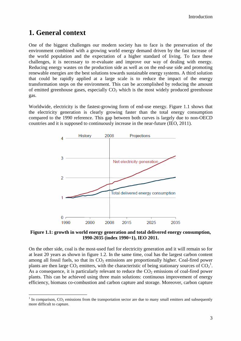
Worldwide, electricity is the fastest-growing form of end-use energy. Figure 1.1 shows that

the electricity generation is clearly growing faster than the total energy consumption

compared to the 1990 reference. This gap between both curves is largely due to non-OECD

countries and it is supposed to continuously increase in the near-future (IEO, 2011).

Figure 1.1: growth in world energy generation and total delivered energy consumption,

1990-2035 (index 1990=1), IEO 2011.

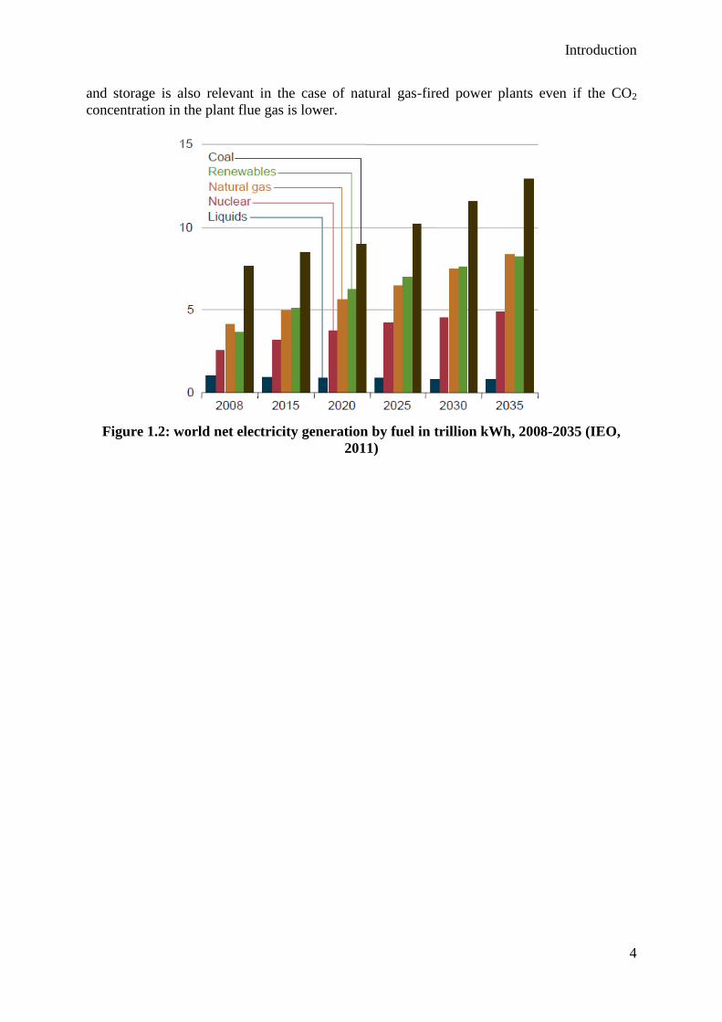
On the other side, coal is the most-used fuel for electricity generation and it will remain so for

at least 20 years as shown in figure 1.2. In the same time, coal has the largest carbon content

among all fossil fuels, so that its CO2 emissions are proportionally higher. Coal-fired power

plants are then large CO2 emitters, with the characteristic of being stationary sources of CO21.

As a consequence, it is particularly relevant to reduce the CO2 emissions of coal-fired power

plants. This can be achieved using three main solutions: continuous improvement of energy

efficiency, biomass co-combustion and carbon capture and storage. Moreover, carbon capture

1 In comparison, CO2 emissions from the transportation sector are due to many small emitters and subsequently

more difficult to capture.

Introduction

4

and storage is also relevant in the case of natural gas-fired power plants even if the CO2

concentration in the plant flue gas is lower.

Figure 1.2: world net electricity generation by fuel in trillion kWh, 2008-2035 (IEO,

2011)

Introduction

5

2. Carbon capture and storage

The goal of carbon capture and storage (CCS) is to capture the carbon dioxide where it is

emitted, to transport it and to store it in geological formations. The captured CO2 remains

underground and does not contribute anymore to the greenhouse gas effect. An alternative

solution to geological storage is the valorization of the captured CO2.

CCS simultaneously faces the reduction of CO2 emissions and the large use of fossil fuels,

lately enhanced by the growing exploitation of unconventional shale gas. One of its main

advantages is that it can be rapidly implemented to mitigate CO2 emissions worldwide. It is

thus a key technology for keeping the CO2 concentration in the atmosphere by 450 ppm, so

that the global temperature rise can be limited to 2°C (WEO 2013). This technology can help

to perform the transition from our carbon-based society with its greenhouse gases emissions

concerns towards a society based on sustainable energy systems. However, long-term use of

CCS is not recommended due to its high energy cost and to the limited availability of fossil

fuels (Piessens et al., 2010).

In the present section, some techniques for capturing CO2 from a flue gas stream are briefly

presented. Three main processes using these techniques are described. Some insight is also

given into transport, valorization and storage of CO2.

2.1 Basic techniques for CO2 capture

The main techniques for CO2 capture are presented in this section. They are techniques for

isolating the carbon dioxide present in a gas stream. In the case of a fossil fuel-fired power

plant, CO2 is captured from a flue gas stream containing mainly nitrogen, water and oxygen,

which are environmentally harmless.

Chemical absorption

The most used CO2 separation technique is the chemical absorption, also called reactive

absorption. This is the preferred technique when the CO2 partial pressure is low,

independently of the process pressure. A chemical reaction takes place between CO2 and the

chemical solvent at moderate or low temperature. This reaction can be reversed by increasing

the temperature. However, the high energy requirement for the solvent regeneration is the

main drawback of this technique.

Many characteristics must be evaluated when looking for an optimal chemical solvent.

Among others, the ideal solvent has a low absorption enthalpy, so that the regeneration is

easier. Its reaction with CO2 is rapid and its CO2 loading capacity important. Furthermore, it

is not toxic or corrosive and it does not degrade in the conditions of the capture process. In the

same time, it degrades to harmless products in case of leakage to the environment. Its vapor

pressure is low to prevent evaporation losses. Last but not least, it is also cheap and

industrially available.

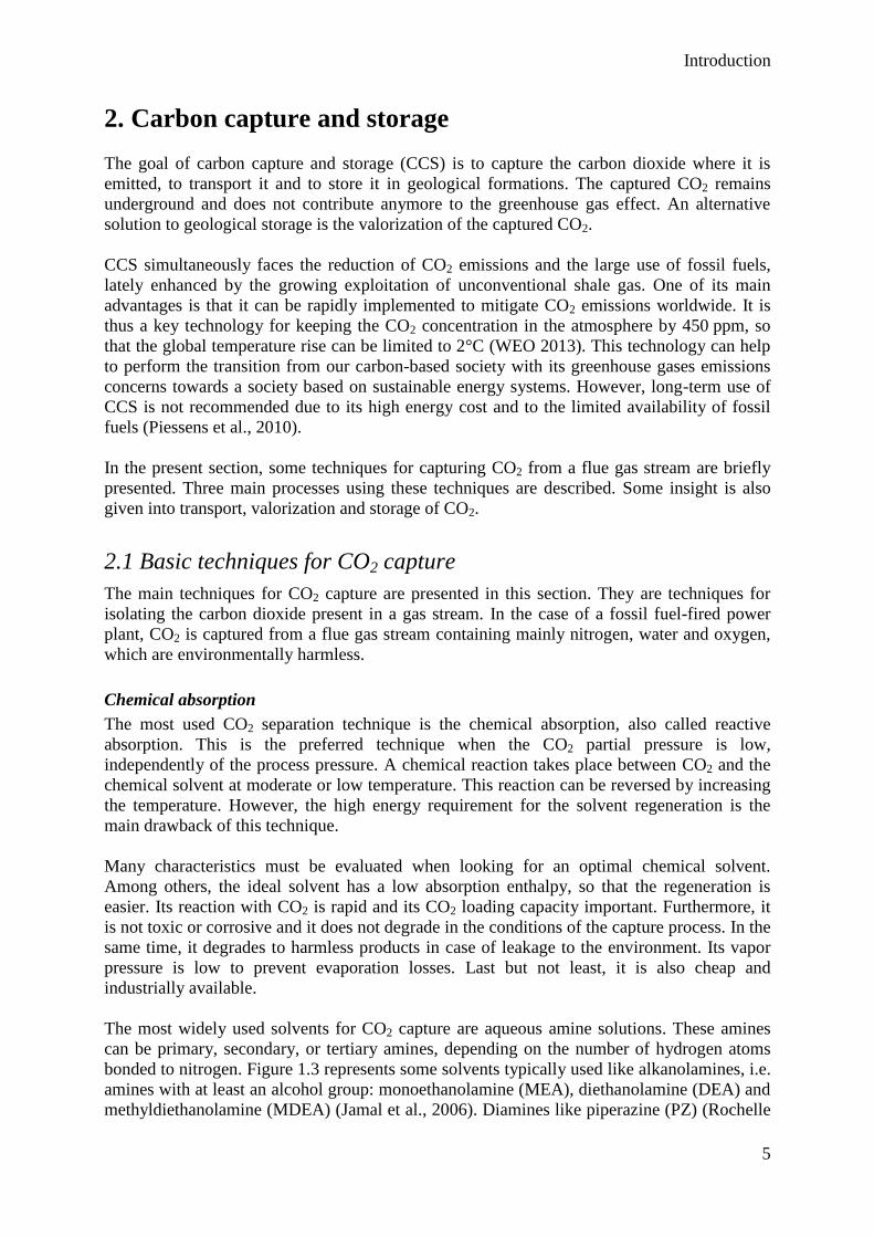
The most widely used solvents for CO2 capture are aqueous amine solutions. These amines

can be primary, secondary, or tertiary amines, depending on the number of hydrogen atoms

bonded to nitrogen. Figure 1.3 represents some solvents typically used like alkanolamines, i.e.

amines with at least an alcohol group: monoethanolamine (MEA), diethanolamine (DEA) and

methyldiethanolamine (MDEA) (Jamal et al., 2006). Diamines like piperazine (PZ) (Rochelle

Introduction

6

et al., 2011) or ethylenediamine (EDA) are also represented, as well as a sterically hindered

amine, 2-amino-2-methylpropanol (AMP).

MEA DEA MDEA

AMP EDA PZ

Figure 1.3: typically used alkanolamines for chemical absorption of CO2

Many alternatives to conventional amine solvents have been proposed in the last decade.

Among them, chilled ammonia (Ciferno et al., 2009) and potassium carbonate (K2CO3)

(Rochelle et al., 2003) have been widely studied. New generations of chemical solvents have

been developed, including amino-acids (Jockenhövel et al., 2009a) and ionic liquids

(Heldebrant et al., 2009). Demixing solvents seem to be another promising alternative, taking

advantage of the phase separation between a CO2 rich loaded amine and a CO2 lean loaded

one (Raynal et al., 2011). However, due to the numerous properties that an ideal solvent

should have, research in this field is still on-going.

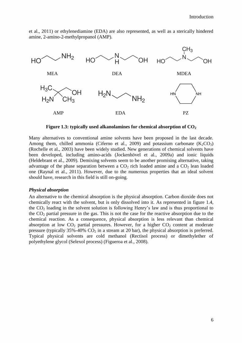
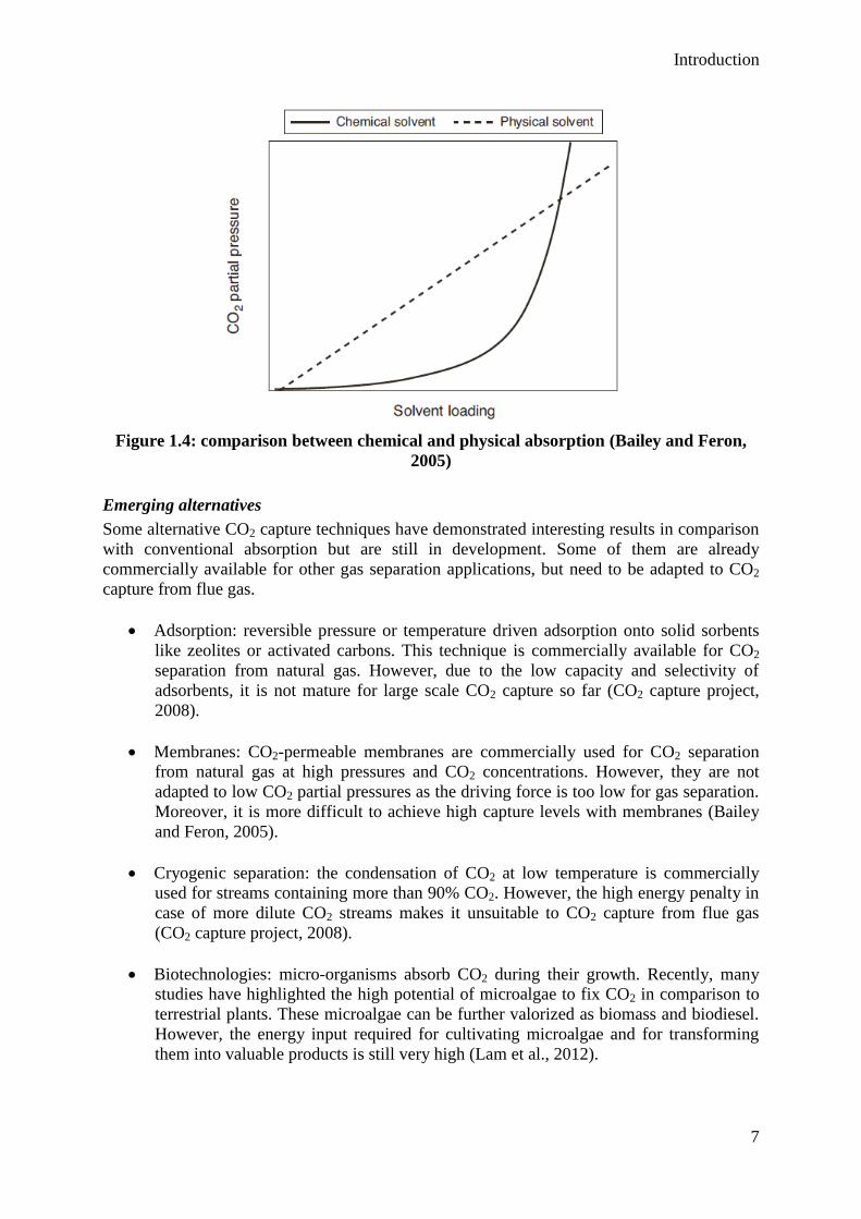
Physical absorption

An alternative to the chemical absorption is the physical absorption. Carbon dioxide does not

chemically react with the solvent, but is only dissolved into it. As represented in figure 1.4,

the CO2 loading in the solvent solution is following Henry’s law and is thus proportional to

the CO2 partial pressure in the gas. This is not the case for the reactive absorption due to the

chemical reaction. As a consequence, physical absorption is less relevant than chemical

absorption at low CO2 partial pressures. However, for a higher CO2 content at moderate

pressure (typically 35%-40% CO2 in a stream at 20 bar), the physical absorption is preferred.

Typical physical solvents are cold methanol (Rectisol process) or dimethylether of

polyethylene glycol (Selexol process) (Figueroa et al., 2008).

Introduction

7

Figure 1.4: comparison between chemical and physical absorption (Bailey and Feron,

2005)

Emerging alternatives

Some alternative CO2 capture techniques have demonstrated interesting results in comparison

with conventional absorption but are still in development. Some of them are already

commercially available for other gas separation applications, but need to be adapted to CO2

capture from flue gas.

Adsorption: reversible pressure or temperature driven adsorption onto solid sorbents

like zeolites or activated carbons. This technique is commercially available for CO2

separation from natural gas. However, due to the low capacity and selectivity of

adsorbents, it is not mature for large scale CO2 capture so far (CO2 capture project,

2008).

Membranes: CO2-permeable membranes are commercially used for CO2 separation

from natural gas at high pressures and CO2 concentrations. However, they are not

adapted to low CO2 partial pressures as the driving force is too low for gas separation.

Moreover, it is more difficult to achieve high capture levels with membranes (Bailey

and Feron, 2005).

Cryogenic separation: the condensation of CO2 at low temperature is commercially

used for streams containing more than 90% CO2. However, the high energy penalty in

case of more dilute CO2 streams makes it unsuitable to CO2 capture from flue gas

(CO2 capture project, 2008).

Biotechnologies: micro-organisms absorb CO2 during their growth. Recently, many

studies have highlighted the high potential of microalgae to fix CO2 in comparison to

terrestrial plants. These microalgae can be further valorized as biomass and biodiesel.

However, the energy input required for cultivating microalgae and for transforming

them into valuable products is still very high (Lam et al., 2012).

Introduction

8

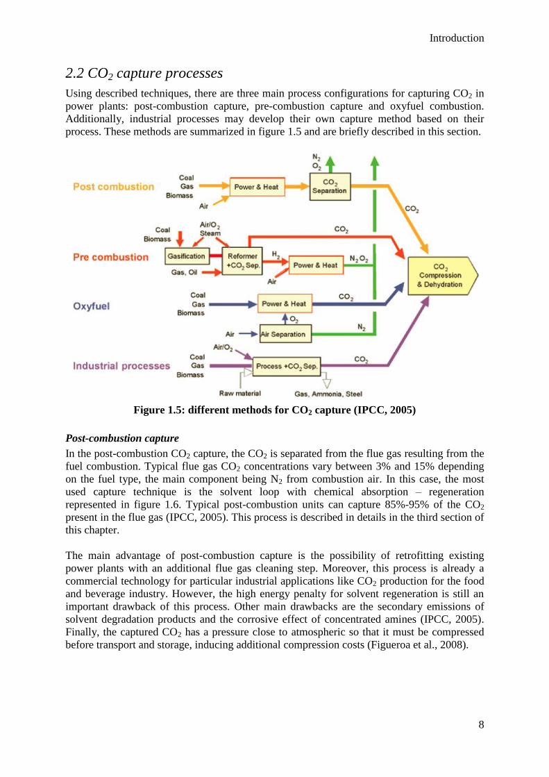
2.2 CO2 capture processes

Using described techniques, there are three main process configurations for capturing CO2 in

power plants: post-combustion capture, pre-combustion capture and oxyfuel combustion.

Additionally, industrial processes may develop their own capture method based on their

process. These methods are summarized in figure 1.5 and are briefly described in this section.

Figure 1.5: different methods for CO2 capture (IPCC, 2005)

Post-combustion capture

In the post-combustion CO2 capture, the CO2 is separated from the flue gas resulting from the

fuel combustion. Typical flue gas CO2 concentrations vary between 3% and 15% depending

on the fuel type, the main component being N2 from combustion air. In this case, the most

used capture technique is the solvent loop with chemical absorption – regeneration

represented in figure 1.6. Typical post-combustion units can capture 85%-95% of the CO2

present in the flue gas (IPCC, 2005). This process is described in details in the third section of

this chapter.

The main advantage of post-combustion capture is the possibility of retrofitting existing

power plants with an additional flue gas cleaning step. Moreover, this process is already a

commercial technology for particular industrial applications like CO2 production for the food

and beverage industry. However, the high energy penalty for solvent regeneration is still an

important drawback of this process. Other main drawbacks are the secondary emissions of

solvent degradation products and the corrosive effect of concentrated amines (IPCC, 2005).

Finally, the captured CO2 has a pressure close to atmospheric so that it must be compressed

before transport and storage, inducing additional compression costs (Figueroa et al., 2008).

Introduction

9

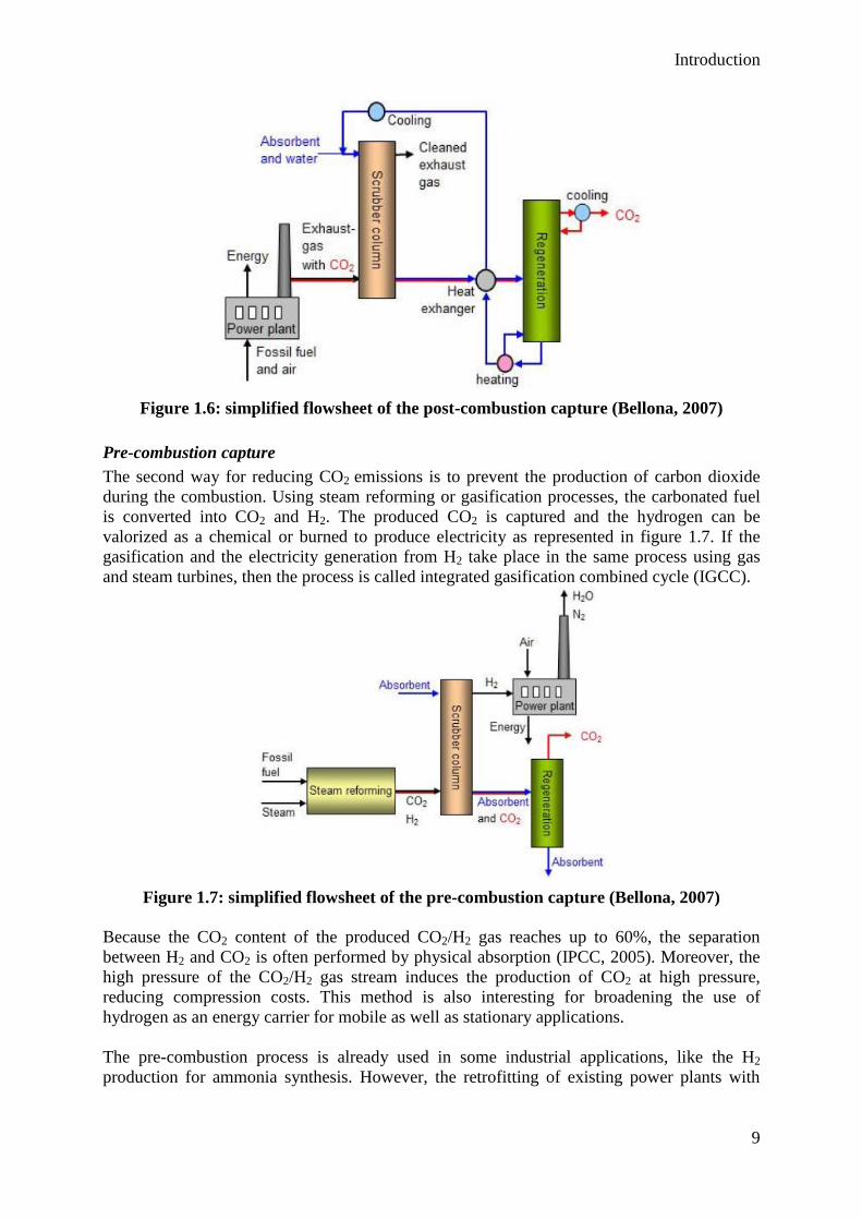
Figure 1.6: simplified flowsheet of the post-combustion capture (Bellona, 2007)

Pre-combustion capture

The second way for reducing CO2 emissions is to prevent the production of carbon dioxide

during the combustion. Using steam reforming or gasification processes, the carbonated fuel

is converted into CO2 and H2. The produced CO2 is captured and the hydrogen can be

valorized as a chemical or burned to produce electricity as represented in figure 1.7. If the

gasification and the electricity generation from H2 take place in the same process using gas

and steam turbines, then the process is called integrated gasification combined cycle (IGCC).

Figure 1.7: simplified flowsheet of the pre-combustion capture (Bellona, 2007)

Because the CO2 content of the produced CO2/H2 gas reaches up to 60%, the separation

between H2 and CO2 is often performed by physical absorption (IPCC, 2005). Moreover, the

high pressure of the CO2/H2 gas stream induces the production of CO2 at high pressure,

reducing compression costs. This method is also interesting for broadening the use of

hydrogen as an energy carrier for mobile as well as stationary applications.

The pre-combustion process is already used in some industrial applications, like the H2

production for ammonia synthesis. However, the retrofitting of existing power plants with

Introduction

10

pre-combustion capture is not applicable (Figueroa et al., 2008) and developing gas turbines

for electricity generation from H2 still remains an important challenge (Bellona, 2013).

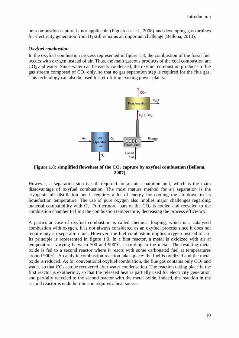
Oxyfuel combustion

In the oxyfuel combustion process represented in figure 1.8, the combustion of the fossil fuel

occurs with oxygen instead of air. Thus, the main gaseous products of the coal combustion are

CO2 and water. Since water can be easily condensed, the oxyfuel combustion produces a flue

gas stream composed of CO2 only, so that no gas separation step is required for the flue gas.

This technology can also be used for retrofitting existing power plants.

Figure 1.8: simplified flowsheet of the CO2 capture by oxyfuel combustion (Bellona,

2007)

However, a separation step is still required for an air-separation unit, which is the main

disadvantage of oxyfuel combustion. The most mature method for air separation is the

cryogenic air distillation but it requires a lot of energy for cooling the air down to its

liquefaction temperature. The use of pure oxygen also implies major challenges regarding

material compatibility with O2. Furthermore, part of the CO2 is cooled and recycled to the

combustion chamber to limit the combustion temperature, decreasing the process efficiency.

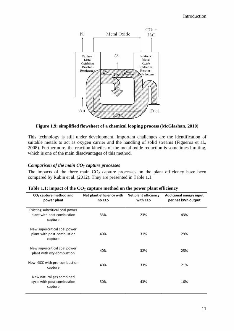
A particular case of oxyfuel combustion is called chemical looping, which is a catalyzed

combustion with oxygen. It is not always considered as an oxyfuel process since it does not

require any air-separation unit. However, the fuel combustion implies oxygen instead of air.

Its principle is represented in figure 1.9. In a first reactor, a metal is oxidized with air at

temperatures varying between 700 and 900°C, according to the metal. The resulting metal

oxide is fed to a second reactor where it reacts with some carbonated fuel at temperatures

around 900°C. A catalytic combustion reaction takes place: the fuel is oxidized and the metal

oxide is reduced. As for conventional oxyfuel combustion, the flue gas contains only CO2 and

water, so that CO2 can be recovered after water condensation. The reaction taking place in the

first reactor is exothermic, so that the released heat is partially used for electricity generation

and partially recycled to the second reactor with the metal oxide. Indeed, the reaction in the

second reactor is endothermic and requires a heat source.

Introduction

11

Figure 1.9: simplified flowsheet of a chemical looping process (McGlashan, 2010)

This technology is still under development. Important challenges are the identification of

suitable metals to act as oxygen carrier and the handling of solid streams (Figueroa et al.,

2008). Furthermore, the reaction kinetics of the metal oxide reduction is sometimes limiting,

which is one of the main disadvantages of this method.

Comparison of the main CO2 capture processes

The impacts of the three main CO2 capture processes on the plant efficiency have been

compared by Rubin et al. (2012). They are presented in Table 1.1.

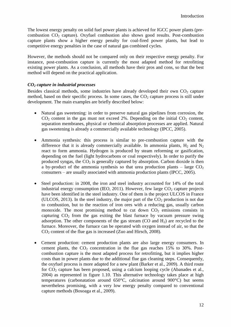
Table 1.1: impact of the CO2 capture method on the power plant efficiency

CO2 capture method and power plant

Net plant efficiency with no CCS

Net plant efficiency with CCS

Additional energy input per net kWh output

Existing subcritical coal power plant with post combustion

capture 33% 23% 43%

New supercritical coal power plant with post-combustion

capture 40% 31% 29%

New supercritical coal power plant with oxy-combustion

40% 32% 25%

New IGCC with pre-combustion capture

40% 33% 21%

New natural gas combined cycle with post-combustion

capture 50% 43% 16%

Introduction

12

The lowest energy penalty on solid fuel power plants is achieved for IGCC power plants (pre-

combustion CO2 capture). Oxyfuel combustion also shows good results. Post-combustion

capture plants show a higher energy penalty for coal-fired power plants, but lead to

competitive energy penalties in the case of natural gas combined cycles.

However, the methods should not be compared only on their respective energy penalty. For

instance, post-combustion capture is currently the most adapted method for retrofitting

existing power plants. As a conclusion, all methods have their pros and cons, so that the best

method will depend on the practical application.

CO2 capture in industrial processes

Besides classical methods, some industries have already developed their own CO2 capture

method, based on their specific process. In some cases, the CO2 capture process is still under

development. The main examples are briefly described below:

Natural gas sweetening: in order to preserve natural gas pipelines from corrosion, the

CO2 content in the gas must not exceed 2%. Depending on the initial CO2 content,

separation membranes, physical or chemical absorption processes are applied. Natural

gas sweetening is already a commercially available technology (IPCC, 2005).

Ammonia synthesis: this process is similar to pre-combustion capture with the

difference that it is already commercially available. In ammonia plants, H2 and N2

react to form ammonia. Hydrogen is produced by steam reforming or gasification,

depending on the fuel (light hydrocarbons or coal respectively). In order to purify the

produced syngas, the CO2 is generally captured by absorption. Carbon dioxide is then

a by-product of the ammonia synthesis so that urea production plants – large CO2

consumers – are usually associated with ammonia production plants (IPCC, 2005).

Steel production: in 2008, the iron and steel industry accounted for 14% of the total

industrial energy consumption (IEO, 2011). However, few large CO2 capture projects

have been identified in the steel industry. One of them is the project ULCOS in France

(ULCOS, 2013). In the steel industry, the major part of the CO2 production is not due

to combustion, but to the reaction of iron ores with a reducing gas, usually carbon

monoxide. The most promising method to cut down CO2 emissions consists in

capturing CO2 from the gas exiting the blast furnace by vacuum pressure swing

adsorption. The other components of the gas stream (CO and H2) are recycled to the

furnace. Moreover, the furnace can be operated with oxygen instead of air, so that the

CO2 content of the flue gas is increased (Zuo and Hirsch, 2008).

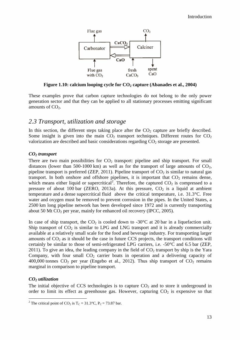
Cement production: cement production plants are also large energy consumers. In

cement plants, the CO2 concentration in the flue gas reaches 15% to 30%. Post-

combustion capture is the most adapted process for retrofitting, but it implies higher

costs than in power plants due to the additional flue gas cleaning steps. Consequently,

the oxyfuel process is more adapted for a new plant (Barker et al., 2009). A third route

for CO2 capture has been proposed, using a calcium looping cycle (Abanades et al.,

2004) as represented in figure 1.10. This alternative technology takes place at high

temperatures (carbonatation around 650°C, calcination around 900°C) but seems

nevertheless promising, with a very low energy penalty compared to conventional

capture methods (Bosoaga et al., 2009).

Introduction

13

Figure 1.10: calcium looping cycle for CO2 capture (Abanades et al., 2004)

These examples prove that carbon capture technologies do not belong to the only power

generation sector and that they can be applied to all stationary processes emitting significant

amounts of CO2.

2.3 Transport, utilization and storage

In this section, the different steps taking place after the CO2 capture are briefly described.

Some insight is given into the main CO2 transport techniques. Different routes for CO2

valorization are described and basic considerations regarding CO2 storage are presented.

CO2 transport

There are two main possibilities for CO2 transport: pipeline and ship transport. For small

distances (lower than 500-1000 km) as well as for the transport of large amounts of CO2,

pipeline transport is preferred (ZEP, 2011). Pipeline transport of CO2 is similar to natural gas

transport. In both onshore and offshore pipelines, it is important that CO2 remains dense,

which means either liquid or supercritical2. Therefore, the captured CO2 is compressed to a

pressure of about 100 bar (ZERO, 2013a). At this pressure, CO2 is a liquid at ambient

temperature and a dense supercritical fluid above the critical temperature, i.e. 31.3°C. Free

water and oxygen must be removed to prevent corrosion in the pipes. In the United States, a

2500 km long pipeline network has been developed since 1972 and is currently transporting

about 50 Mt CO2 per year, mainly for enhanced oil recovery (IPCC, 2005).

In case of ship transport, the CO2 is cooled down to -30°C at 20 bar in a liquefaction unit.

Ship transport of CO2 is similar to LPG and LNG transport and it is already commercially

available at a relatively small scale for the food and beverage industry. For transporting larger

amounts of CO2 as it should be the case in future CCS projects, the transport conditions will

certainly be similar to those of semi-refrigerated LPG carriers, i.e. -50°C and 6.5 bar (ZEP,

2011). To give an idea, the leading company in the field of CO2 transport by ship is the Yara

Company, with four small CO2 carrier boats in operation and a delivering capacity of

400,000 tonnes CO2 per year (Engebo et al., 2012). Thus ship transport of CO2 remains

marginal in comparison to pipeline transport.

CO2 utilization

The initial objective of CCS technologies is to capture CO2 and to store it underground in

order to limit its effect as greenhouse gas. However, capturing CO2 is expensive so that

2 The critical point of CO2 is TC = 31.3°C, PC = 73.87 bar.

Introduction

14

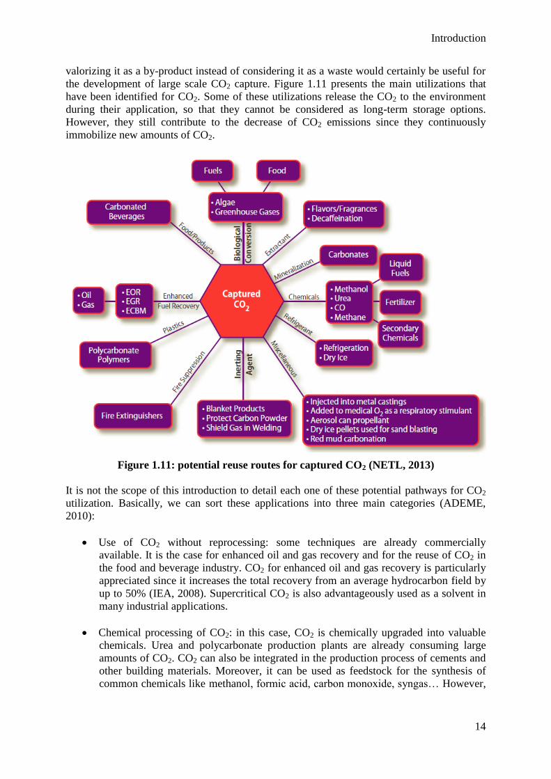
valorizing it as a by-product instead of considering it as a waste would certainly be useful for

the development of large scale CO2 capture. Figure 1.11 presents the main utilizations that

have been identified for CO2. Some of these utilizations release the CO2 to the environment

during their application, so that they cannot be considered as long-term storage options.

However, they still contribute to the decrease of CO2 emissions since they continuously

immobilize new amounts of CO2.

Figure 1.11: potential reuse routes for captured CO2 (NETL, 2013)

It is not the scope of this introduction to detail each one of these potential pathways for CO2

utilization. Basically, we can sort these applications into three main categories (ADEME,

2010):

Use of CO2 without reprocessing: some techniques are already commercially

available. It is the case for enhanced oil and gas recovery and for the reuse of CO2 in

the food and beverage industry. CO2 for enhanced oil and gas recovery is particularly

appreciated since it increases the total recovery from an average hydrocarbon field by

up to 50% (IEA, 2008). Supercritical CO2 is also advantageously used as a solvent in

many industrial applications.

Chemical processing of CO2: in this case, CO2 is chemically upgraded into valuable

chemicals. Urea and polycarbonate production plants are already consuming large

amounts of CO2. CO2 can also be integrated in the production process of cements and

other building materials. Moreover, it can be used as feedstock for the synthesis of

common chemicals like methanol, formic acid, carbon monoxide, syngas… However,

Introduction

15

this upgrading of CO2 always requires energy, so that these processes are

economically viable only in a few cases so far (ADEME, 2010).

Biological processing of CO2: as an alternative to chemical processes for upgrading

CO2, biological processes use sunlight as a cheap and sustainable source of energy.

Microalgae have a promising potential in capturing CO2 and can be processed into

various products, including food, fuel and chemicals. The main challenge of this reuse

route is the high energy input for the biomass transformation into chemicals. CO2 is

also sometimes used for growth enhancement in greenhouse cultures (Yara, 2013).

The large number and the diversity of the reuse routes for captured CO2 seem very promising.

This would convert CCS to CCUS, i.e. carbon capture, utilization and storage (CSLF, 2011).

Indeed, a recent study has estimated that the various ways of CO2 utilization have the

potential of reducing CO2 emissions by 3.7 Gton per year, equivalent to about 10% of the

current annual emissions (Sridhar and Hill, 2011). Finally, reusing CO2 could contribute not

only to the reduction of greenhouse gas emissions, but also to a sustainable society by the

development of new economic activities.

CO2 storage

In the case of large scale implementation of CCS, gigantic amounts of CO2 would be

captured, so that the major part of the captured CO2 could not be reused but would be injected

underground. In geological structures, CO2 dissolve and progressively mineralize to carbonate

over several thousands of years. Different geological formations are studied for CO2 storage

(IPCC 2005):

(Depleted) oil and gas fields: this is related to the enhanced hydrocarbon recovery

technology which is already a mature technology.

Unmineable coal beds: CO2 storage in coal seams has a limited capacity potential, so

that it can be considered as a local solution only. However, it can gain interest if

recovering methane from coal layers is achievable by CO2 injection.

Deep saline aquifers: saline formations have the largest storage capacities but they

have been less studied than hydrocarbon fields. The Sleipner project in the North Sea

is the most famous example of CO2 storage in saline formations. Since 1996, about

1 Mt CO2 has been injected each year at Sleipner.

A geological structure for CO2 storage must satisfy three main characteristics (Cooper, 2009).

Firstly, its capacity must be sufficient, which is related to its size but first of all to the porosity

of its rock. Secondly, the rock permeability must allow the injection of CO2. And thirdly, a

gas tight cap rock formation must preserve the containment of the injected fluid. The storage

site should also be located at a minimal depth of 800m to ensure supercritical conditions for

efficient CO2 storage. To minimize transport costs, it should also be as close as possible to

CO2 emission sources.

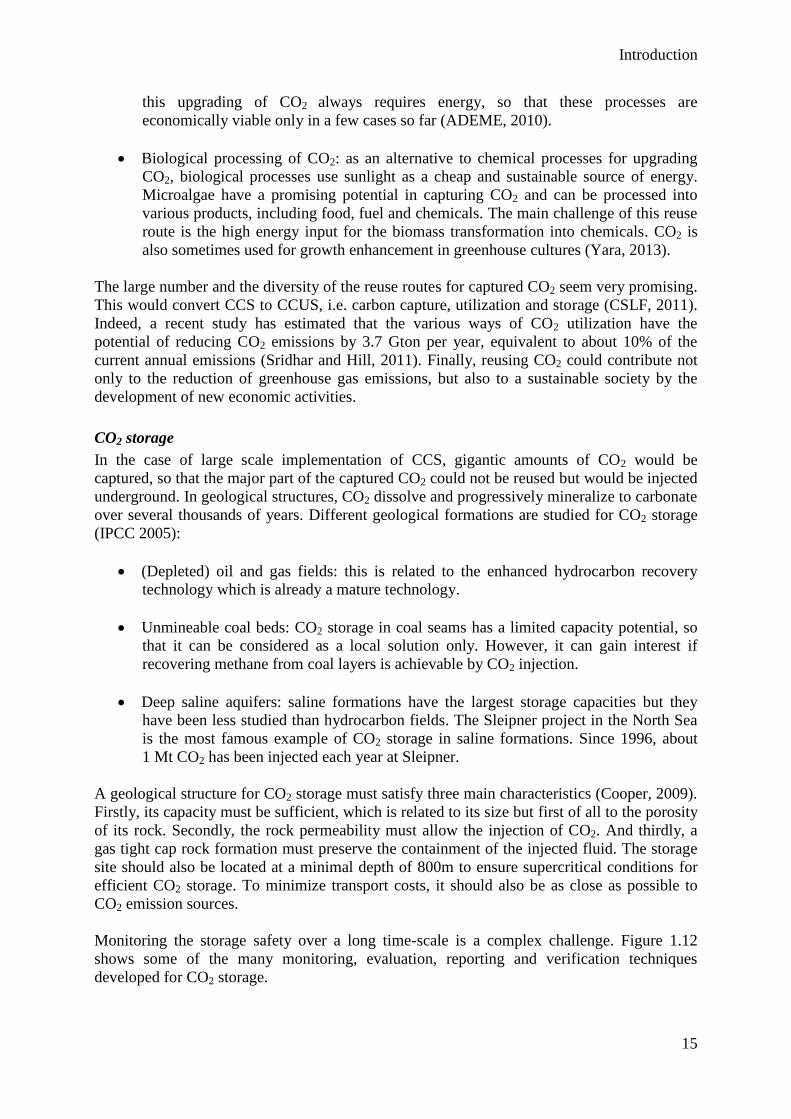
Monitoring the storage safety over a long time-scale is a complex challenge. Figure 1.12

shows some of the many monitoring, evaluation, reporting and verification techniques

developed for CO2 storage.

Introduction

16

Figure 1.12: monitoring techniques for CO2 storage (CO2 capture project, 2013)

Although the time scale is very different, geological storage of CO2 presents many similarities

with natural gas storage which is already a commercial technology. Natural gas storage acts

as a seasonal buffer for the distribution network: natural gas is stored in summer when the

demand is low and is recovered in winter when the demand increases (Fluxys, 2013). Storage

sites should also cope with any interruption of the natural gas delivery due to geopolitical

issues or to technical incidents. Consequently, experience from natural gas storage may be

useful for CO2 storage.

In conclusion, the different CO2 capture methods are part of a much larger process that

includes transport, reuse of CO2, storage, monitoring… To give a complete overview on CCS

(or rather CCUS), many non-technical considerations should also be mentioned, including

economic challenges, geopolitical considerations, public perception… These subjects will not

be described in the framework of this work, but more information about them can be found in

the scientific literature.

Introduction

17

3. Post-combustion capture with amine solvents

In the previous section, the main principles of carbon capture, utilization and storage have

been presented. In this section, the focus is set on the post-combustion CO2 capture by

reactive absorption in amine solvents, which is the object of the present work. First, the

process is described. Then, a list of existing pilot and commercial installations is presented.

Finally, advantages and drawbacks of this technology are discussed.

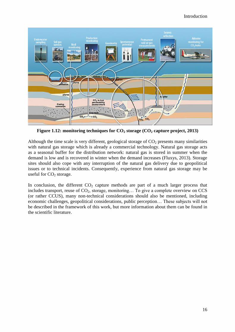
3.1 Process description

The benchmark solvent for the CO2 reactive absorption is an aqueous solution of 30 wt%

monoethanolamine (MEA, HO-CH2-CH2-NH2). The principle of this process is represented in

figure 1.13.

Figure 1.13: flowsheet of the chemical absorption process (Sintef, 2013)

In the case of a coal power plant, the flue gas contains3 14% CO2, 6% O2, 12% H2O and 68%

N2 (Laborelec, 2009). Different gas cleaning steps (not represented in figure 1.13) are

necessary to remove impurities from the flue gas before CO2 separation. Among others, sulfur

oxides can be almost completely removed by flue gas desulfurization (FGD) and nitrous

oxides by selective catalytic reduction (SCR). Thus, a wet pre-scrubbing treatment removes

any remaining SO2 and brings the flue gas to the desired temperature before CO2 capture.

After a compression step, the flue gas enters the absorption column or absorber. Carbon

dioxide reacts with the amine solvent at temperatures varying between 40 and 60°C (~55°C in

the case of MEA). This chemical absorption is an exothermic reaction. The absorption

3 Volume percentages. To give an idea, flue gas from natural gas fired power plants contains 7-10% CO2, and

flue gas from combined cycle gas turbine contains 3-4% CO2 (volume fraction on a dry basis) (IPCC, 2007).

Introduction

18

mechanism in the solvent can be summarized in two main steps: formation of a zwitterion

(1.1) and instantaneous removal of a proton by a base B to form a carbamate (1.2). In aqueous

solutions, the base B can be either water, an amine molecule or an OH- ion. Reaction 1.1 is

rate-determining (Danckwerts, 1979; Versteeg and Van Swaaij, 1988).

HO-CH2-CH2-NH2 + CO2 ↔ HO-CH2-CH2-NH-COO- H

+ (1.1)

HO-CH2-CH2-NH-COO- H

+ + B ↔ HO-CH2-CH2-NH-COO

- + BH

+ (1.2)

After the absorption, the treated flue gas usually flows through a water-wash section to reduce

the emissions of volatile solvent and degradation products. The washing section also regulates

the temperature of the flue gas in order to control the amount of water exiting the process. A

demister is also installed to prevent the emission of liquid droplets. The CO2-loaded solvent

(also referred to as “rich solvent”) is pumped to a regeneration column (also named

“stripper”) via a heat-exchanger where the rich solvent is pre-heated.

In the stripper, the solvent is regenerated at temperatures varying between 100 and 140°C

(~120°C in the case of MEA). The purpose of the reboiler at the stripper bottom is to supply

thermal energy for the solvent regeneration4. At this temperature, the absorption reaction is

reversed, so that CO2 is released from the solvent. The regenerated solvent (“lean solvent”) is

fed back to the absorber via the rich-lean heat exchanger where it pre-heats the rich solvent. A

further heat exchanger cools the regenerated solvent down to the desired absorber entrance

temperature.

The gaseous CO2 stream after desorption contains some water that is recycled to the process

by condensation, so that the final product may reach a CO2-purity of 99% by volume. Finally,

the objective that is generally pursued in post-combustion processes is the removal of 90% of

the CO2 present in the power plant flue gas stream (Laborelec, 2009).

3.2 Main post-combustion capture projects

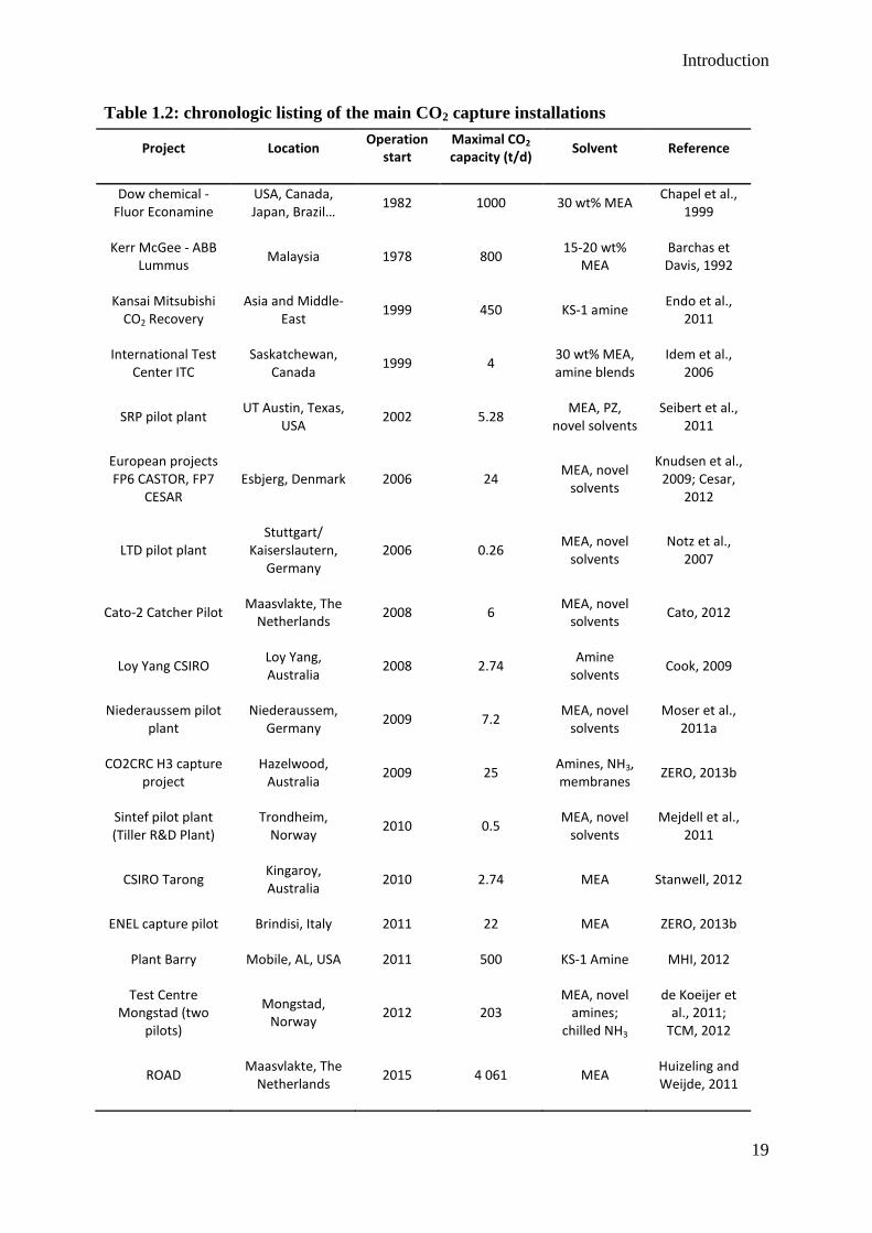
Table 1.2 lists the main post-combustion CO2 capture installations using amine solvents. The

first commercial capture plants were designed more than 30 years ago for commercial CO2

production. The intensive research on post-combustion CO2 capture for environmental

purpose has started in the 2000ies. Different pilot installations have been developed around

the world, with varying scale and objectives.

4 This heat is supplied under the form of low-pressure steam from the power plant. The steam is preferentially

extracted at the cross-over pipe between the intermediate and low pressure steam turbines (Jockenhövel et al.,

2009b).

Introduction

19

Table 1.2: chronologic listing of the main CO2 capture installations

Project Location Operation

start Maximal CO2 capacity (t/d)

Solvent Reference

Dow chemical - Fluor Econamine

USA, Canada, Japan, Brazil…

1982 1000 30 wt% MEA Chapel et al.,

1999

Kerr McGee - ABB Lummus

Malaysia 1978 800 15-20 wt%

MEA Barchas et Davis, 1992

Kansai Mitsubishi CO2 Recovery

Asia and Middle-East

1999 450 KS-1 amine Endo et al.,

2011

International Test Center ITC

Saskatchewan, Canada

1999 4 30 wt% MEA, amine blends

Idem et al., 2006

SRP pilot plant UT Austin, Texas,

USA 2002 5.28

MEA, PZ, novel solvents

Seibert et al., 2011

European projects FP6 CASTOR, FP7

CESAR Esbjerg, Denmark 2006 24

MEA, novel solvents

Knudsen et al., 2009; Cesar,

2012

LTD pilot plant Stuttgart/

Kaiserslautern, Germany

2006 0.26 MEA, novel

solvents Notz et al.,

2007

Cato-2 Catcher Pilot Maasvlakte, The

Netherlands 2008 6

MEA, novel solvents

Cato, 2012

Loy Yang CSIRO Loy Yang, Australia

2008 2.74 Amine

solvents Cook, 2009

Niederaussem pilot plant

Niederaussem, Germany

2009 7.2 MEA, novel

solvents Moser et al.,

2011a

CO2CRC H3 capture project

Hazelwood, Australia

2009 25 Amines, NH3, membranes

ZERO, 2013b

Sintef pilot plant (Tiller R&D Plant)

Trondheim, Norway

2010 0.5 MEA, novel

solvents Mejdell et al.,

2011

CSIRO Tarong Kingaroy, Australia

2010 2.74 MEA Stanwell, 2012

ENEL capture pilot Brindisi, Italy 2011 22 MEA ZERO, 2013b

Plant Barry Mobile, AL, USA 2011 500 KS-1 Amine MHI, 2012

Test Centre Mongstad (two

pilots)

Mongstad, Norway

2012 203 MEA, novel

amines; chilled NH3

de Koeijer et al., 2011;

TCM, 2012

ROAD Maasvlakte, The

Netherlands 2015 4 061 MEA

Huizeling and Weijde, 2011

Introduction

20

It appears from this list that the largest post-combustion capture installations have been

designed for commercial CO2 production more than ten years ago. The largest modern facility

for CO2 capture in Plant Barry uses a proprietary amine solvent, KS-1. For comparison

purpose, the ROAD project has been mentioned even if not operational yet. This is one of

many large-scale demonstration projects that have been planned recently but its realization is

still uncertain. In the last years, many demonstration projects have been delayed or cancelled

due to cost considerations (Rubin et al., 2012). However, there remains a critical need for

demonstration projects to prove the technical and economic feasibility of large-scale CO2

capture.

3.3 Advantages and drawbacks of post-combustion capture with

amine solvents

The main advantage of CO2 post-combustion capture is its availability for retrofitting existing

power plants (Figueroa et al., 2008). Among the different post-combustion techniques and at

the current state of technology, reactive absorption in amine solvents is often considered as

the most efficient method for CO2 capture, or at least the most feasible route to large-scale

implementation (Rubin et al., 2012; Svendsen et al., 2011). The main reason for that is the

large experience gained in various applications like natural gas sweetening or commercial

CO2 capture from flue gas. Moreover, the development of CO2 capture with amine solvents

was based on MEA, an amine that rapidly reacts with CO2 and has a high CO2 capacity on a

mass basis (Brúder and Svendsen, 2012). However, two main drawbacks still affect the CO2

chemical absorption in amine solvents, and especially in MEA: the high energy requirement

of the process and its environmental safety (Svendsen et al., 2011).

In the case of a new supercritical pulverized coal power plant with post-combustion capture,

the overall plant efficiency drops from 40% to 31%. This corresponds to an additional energy

input of 29% per net kWh output (Rubin et al., 2012). It is thus easy to understand that many

studies on CO2 capture have mainly focused on the reduction of the process energy penalty.

This has been partially achieved by using newly developed solvents and/or alternative process

configurations (among others Mimura et al., 1995; Chakma 1997; Rochelle et al., 2011;

Knudsen et al., 2011).

However the environmental safety of post-combustion capture with amine solvents also

represents a critical issue. Creating a new environmental problem when solving an initial one

must be strictly avoided (Svendsen et al., 2011). Two types of environmentally harmful

chemicals may be emitted by the CO2 capture process: the amine solvent and its degradation

products.

The vapor pressure of amine solvent above its aqueous solutions can be significant, so that

some amine may exit the process with the cleaned flue gas. In the case of MEA, solvent

emissions can be kept very low by an optimal operation of the washing section (Mertens et

al., 2012; Moser et al., 2011b). In comparison, significant emissions of AMP solvent were

recorded during a pilot plant test with AMP/PZ (Mertens et al., 2012). This is in accordance

with the higher volatility of AMP compared to MEA and PZ (Nguyen et al., 2010). Thus,

volatility is a further essential parameter when selecting a new solvent. Based on own

unpublished data, Svendsen et al. (2011) claim that optimal washing sections could bring

amine emissions down to 0.01-0.05 ppm.

Introduction

21

Amine degradation products may also be emitted by the capture process. Indeed, during the

absorption, the amine solvent is in contact with oxygen from the flue gas, inducing oxidative

degradation of the amine. It is also heated in presence of CO2 during the regeneration,

inducing thermal degradation with CO2. If SOx and NOx impurities have not been correctly

removed from the flue gas before the absorber, they may also cause amine solvent

degradation. The amine solvent can degrade into gaseous as well as liquid degradation

products that are classified as environmentally harmful emissions. Some recent studies at lab

and pilot scale have evidenced that the operating conditions of the capture process have a

direct impact on the formation and emission of degradation products (among others Mertens

et al., 2012; Voice and Rochelle, 2013). However, there still remains a knowledge gap about

the environmental impact of post-combustion CO2 capture with amines (Shao and Stangeland,

2009).

Introduction

22

4. Objectives

The main objective of this thesis is to gain a better understanding of the complex mutual

influences between amine solvent degradation and CO2 capture process. This objective

proceeds through two complementary approaches and their combination represents the main

originality of this work.

The first approach is the experimental study of amine solvent degradation. The objective is to

test the influence on degradation of operating parameters like temperature, agitation rate and

flue gas composition. The influence of dissolved metals and degradation inhibitors in the

solvent solution may also be studied since they may affect the degradation rate. However,

amine degradation is a slow phenomenon and it is necessary to accelerate it for collecting data

in a reasonable time framework. The main objectives of this task are the following:

Design and construction of a test rig for accelerating solvent degradation.

Development of analytical methods to characterize degraded solvents.

Evaluation of the relevance of accelerated degradation conditions.

Evaluation of the influence of operating parameters on degradation pathways.

Quantification of the influence of operating parameters on the degradation rate.

Quantification of the influence of dissolved metals and degradation inhibitors on the

degradation rate.

The second approach is the simulation and optimization of the post-combustion CO2 capture

process with amine solvents. The Aspen Plus®

software (Advanced System for Process

Engineering) has been selected as a powerful simulation tool to model CO2 capture. The main

objectives of this task are the following:

Development of a model for the simulation of the post-combustion capture process in

static and dynamic operation modes.

Evaluation of the relevance of this model to simulate industrial processes.

Identification of process parameters having a large influence on the energy

requirement of the CO2 capture.

Evaluation of alternative process configurations.

Propositions for an optimal design of the CO2 capture process.

Finally, the objective of this thesis is to combine both experimental and modeling approaches

in order to develop a model of CO2 capture taking solvent degradation into account. This is

the main originality of this work. Indeed, available models focused so far on the reduction of

the process energy penalty but only few of them did consider the impact of operating

conditions on the process environmental penalty.

Introduction

23

In the present work, the developed methodology is based on the current benchmark solvent

for CO2 capture, i.e. aqueous 30 wt% MEA. Developing a model for CO2 capture that

includes experimental degradation results should give a better understanding of the complex

interactions between amine solvent degradation and process operating conditions. Finally, the

objective is to propose optimal operating conditions that achieve a trade-off between energy

and environmental penalties of post-combustion CO2 capture.

This thesis has been performed in industrial partnership with the company Laborelec, member

of the GDF SUEZ group. Laborelec is a Belgian technical competence center in energy

processes and energy uses. It has been created in 1962 to offer technical expertise to

Electrabel, the main electricity supplier in Belgium (Laborelec, 2009). Its interest for CO2

capture is motivated by the objective of providing technical support to power plant operators

in future CO2 capture installations.

Chapter II

Experimental study of amine solvent degradation

“I think that in the description of natural problems we ought to begin not with the Scriptures,

but with experiments, and demonstrations.”

Galileo Galilei

Experimental study of amine solvent degradation

25

1. Introduction

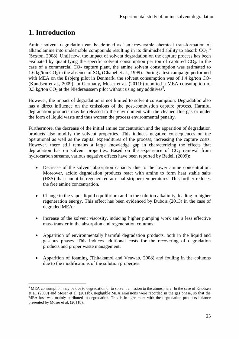
Amine solvent degradation can be defined as “an irreversible chemical transformation of

alkanolamine into undesirable compounds resulting in its diminished ability to absorb CO2.”

(Sexton, 2008). Until now, the impact of solvent degradation on the capture process has been

evaluated by quantifying the specific solvent consumption per ton of captured CO2. In the

case of a commercial CO2 capture plant, the amine solvent consumption was estimated to

1.6 kg/ton CO2 in the absence of SOx (Chapel et al., 1999). During a test campaign performed

with MEA on the Esbjerg pilot in Denmark, the solvent consumption was of 1.4 kg/ton CO2

(Knudsen et al., 2009). In Germany, Moser et al. (2011b) reported a MEA consumption of

0.3 kg/ton CO2 at the Niederaussem pilot without using any additives5.

However, the impact of degradation is not limited to solvent consumption. Degradation also

has a direct influence on the emissions of the post-combustion capture process. Harmful

degradation products may be released to the environment with the cleaned flue gas or under

the form of liquid waste and thus worsen the process environmental penalty.

Furthermore, the decrease of the initial amine concentration and the apparition of degradation

products also modify the solvent properties. This induces negative consequences on the

operational as well as the capital expenditures of the process, increasing the capture costs.

However, there still remains a large knowledge gap in characterizing the effects that

degradation has on solvent properties. Based on the experience of CO2 removal from

hydrocarbon streams, various negative effects have been reported by Bedell (2009):

Decrease of the solvent absorption capacity due to the lower amine concentration.

Moreover, acidic degradation products react with amine to form heat stable salts

(HSS) that cannot be regenerated at usual stripper temperatures. This further reduces

the free amine concentration.

Change in the vapor-liquid equilibrium and in the solution alkalinity, leading to higher

regeneration energy. This effect has been evidenced by Dubois (2013) in the case of

degraded MEA.

Increase of the solvent viscosity, inducing higher pumping work and a less effective

mass transfer in the absorption and regeneration columns.

Apparition of environmentally harmful degradation products, both in the liquid and

gaseous phases. This induces additional costs for the recovering of degradation

products and proper waste management.

Apparition of foaming (Thitakamol and Veawab, 2008) and fouling in the columns

due to the modifications of the solution properties.

5 MEA consumption may be due to degradation or to solvent emission to the atmosphere. In the case of Knudsen

et al. (2009) and Moser et al. (2011b), negligible MEA emissions were recorded in the gas phase, so that the

MEA loss was mainly attributed to degradation. This is in agreement with the degradation products balance

presented by Moser et al. (2011b).

Experimental study of amine solvent degradation

26

Increase of the solution corrosivity due to the presence of acids and chelating agents

among the degradation products. This last point has an impact on the choice of the

pipe and column materials, and consequently on the capital costs.

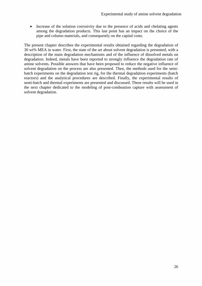
The present chapter describes the experimental results obtained regarding the degradation of

30 wt% MEA in water. First, the state of the art about solvent degradation is presented, with a

description of the main degradation mechanisms and of the influence of dissolved metals on

degradation. Indeed, metals have been reported to strongly influence the degradation rate of

amine solvents. Possible answers that have been proposed to reduce the negative influence of

solvent degradation on the process are also presented. Then, the methods used for the semi-

batch experiments on the degradation test rig, for the thermal degradation experiments (batch

reactors) and the analytical procedures are described. Finally, the experimental results of

semi-batch and thermal experiments are presented and discussed. These results will be used in

the next chapter dedicated to the modeling of post-combustion capture with assessment of

solvent degradation.

Experimental study of amine solvent degradation

27

2. State of the art

In this section, the different degradation mechanisms are described. Then, a summary of the

main research studies performed in the field of MEA degradation is presented. The influence

of dissolved metals on solvent degradation is also discussed. Finally, current solutions to

reduce the negative effects of degradation are presented.

2.1 Degradation mechanisms

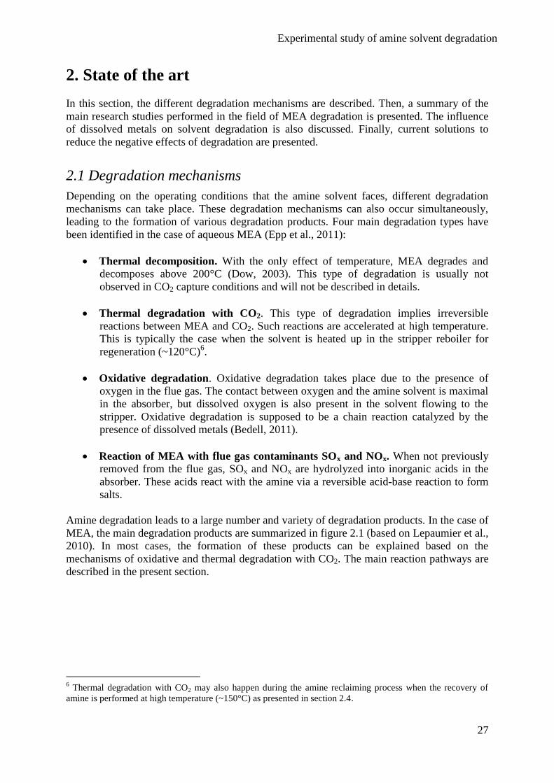
Depending on the operating conditions that the amine solvent faces, different degradation

mechanisms can take place. These degradation mechanisms can also occur simultaneously,

leading to the formation of various degradation products. Four main degradation types have

been identified in the case of aqueous MEA (Epp et al., 2011):

Thermal decomposition. With the only effect of temperature, MEA degrades and

decomposes above 200°C (Dow, 2003). This type of degradation is usually not

observed in CO2 capture conditions and will not be described in details.

Thermal degradation with CO2. This type of degradation implies irreversible

reactions between MEA and CO2. Such reactions are accelerated at high temperature.

This is typically the case when the solvent is heated up in the stripper reboiler for

regeneration (~120°C)6.

Oxidative degradation. Oxidative degradation takes place due to the presence of

oxygen in the flue gas. The contact between oxygen and the amine solvent is maximal

in the absorber, but dissolved oxygen is also present in the solvent flowing to the

stripper. Oxidative degradation is supposed to be a chain reaction catalyzed by the

presence of dissolved metals (Bedell, 2011).

Reaction of MEA with flue gas contaminants SOx and NOx. When not previously

removed from the flue gas, SOx and NOx are hydrolyzed into inorganic acids in the

absorber. These acids react with the amine via a reversible acid-base reaction to form

salts.

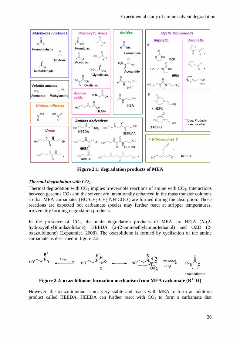
Amine degradation leads to a large number and variety of degradation products. In the case of

MEA, the main degradation products are summarized in figure 2.1 (based on Lepaumier et al.,

2010). In most cases, the formation of these products can be explained based on the

mechanisms of oxidative and thermal degradation with CO2. The main reaction pathways are

described in the present section.

6 Thermal degradation with CO2 may also happen during the amine reclaiming process when the recovery of

amine is performed at high temperature (~150°C) as presented in section 2.4.

Experimental study of amine solvent degradation

28

Figure 2.1: degradation products of MEA

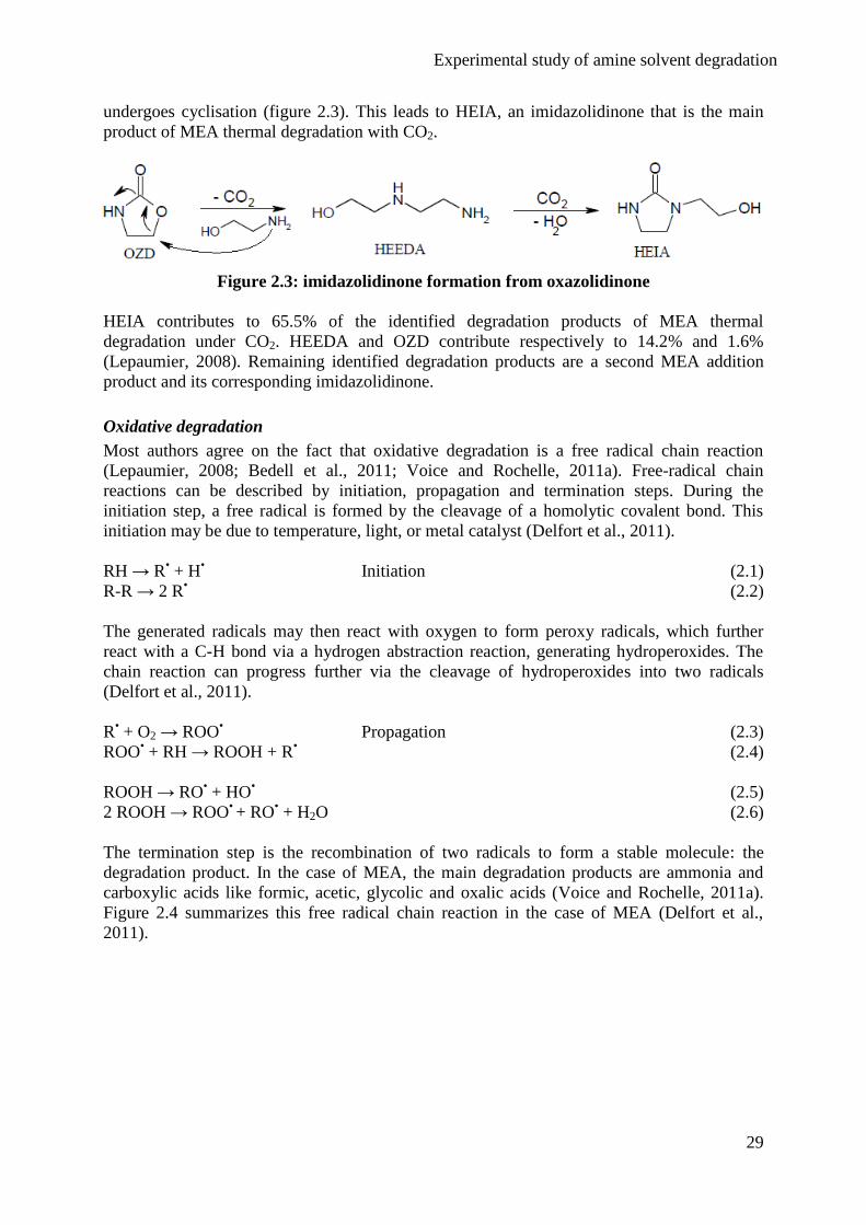
Thermal degradation with CO2

Thermal degradation with CO2 implies irreversible reactions of amine with CO2. Interactions

between gaseous CO2 and the solvent are intentionally enhanced in the mass transfer columns

so that MEA carbamates (HO-CH2-CH2-NH-COO-) are formed during the absorption. Those

reactions are expected but carbamate species may further react at stripper temperatures,

irreversibly forming degradation products.

In the presence of CO2, the main degradation products of MEA are HEIA (N-(2-

hydroxyethyl)imidazolidone), HEEDA (2-(2-aminoethylamino)ethanol) and OZD (2-

oxazolidinone) (Lepaumier, 2008). The oxazolidone is formed by cyclisation of the amine

carbamate as described in figure 2.2.

Figure 2.2: oxazolidinone formation mechanism from MEA carbamate (R1=H)

However, the oxazolidinone is not very stable and reacts with MEA to form an addition

product called HEEDA. HEEDA can further react with CO2 to form a carbamate that

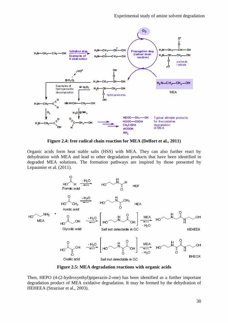
Experimental study of amine solvent degradation

29

undergoes cyclisation (figure 2.3). This leads to HEIA, an imidazolidinone that is the main

product of MEA thermal degradation with CO2.

Figure 2.3: imidazolidinone formation from oxazolidinone

HEIA contributes to 65.5% of the identified degradation products of MEA thermal

degradation under CO2. HEEDA and OZD contribute respectively to 14.2% and 1.6%

(Lepaumier, 2008). Remaining identified degradation products are a second MEA addition

product and its corresponding imidazolidinone.

Oxidative degradation

Most authors agree on the fact that oxidative degradation is a free radical chain reaction

(Lepaumier, 2008; Bedell et al., 2011; Voice and Rochelle, 2011a). Free-radical chain

reactions can be described by initiation, propagation and termination steps. During the

initiation step, a free radical is formed by the cleavage of a homolytic covalent bond. This

initiation may be due to temperature, light, or metal catalyst (Delfort et al., 2011).

RH → R• + H

• Initiation (2.1)

R-R → 2 R• (2.2)

The generated radicals may then react with oxygen to form peroxy radicals, which further

react with a C-H bond via a hydrogen abstraction reaction, generating hydroperoxides. The

chain reaction can progress further via the cleavage of hydroperoxides into two radicals

(Delfort et al., 2011).

R• + O2 → ROO

• Propagation (2.3)

ROO• + RH → ROOH + R

• (2.4)

ROOH → RO• + HO

• (2.5)

2 ROOH → ROO• + RO

• + H2O (2.6)

The termination step is the recombination of two radicals to form a stable molecule: the

degradation product. In the case of MEA, the main degradation products are ammonia and

carboxylic acids like formic, acetic, glycolic and oxalic acids (Voice and Rochelle, 2011a).

Figure 2.4 summarizes this free radical chain reaction in the case of MEA (Delfort et al.,

2011).

Experimental study of amine solvent degradation

30

Figure 2.4: free radical chain reaction for MEA (Delfort et al., 2011)

Organic acids form heat stable salts (HSS) with MEA. They can also further react by

dehydration with MEA and lead to other degradation products that have been identified in

degraded MEA solutions. The formation pathways are inspired by those presented by

Lepaumier et al. (2011).

Figure 2.5: MEA degradation reactions with organic acids

Then, HEPO (4-(2-hydroxyethyl)piperazin-2-one) has been identified as a further important

degradation product of MEA oxidative degradation. It may be formed by the dehydration of

HEHEEA (Strazisar et al., 2003).

Experimental study of amine solvent degradation

31

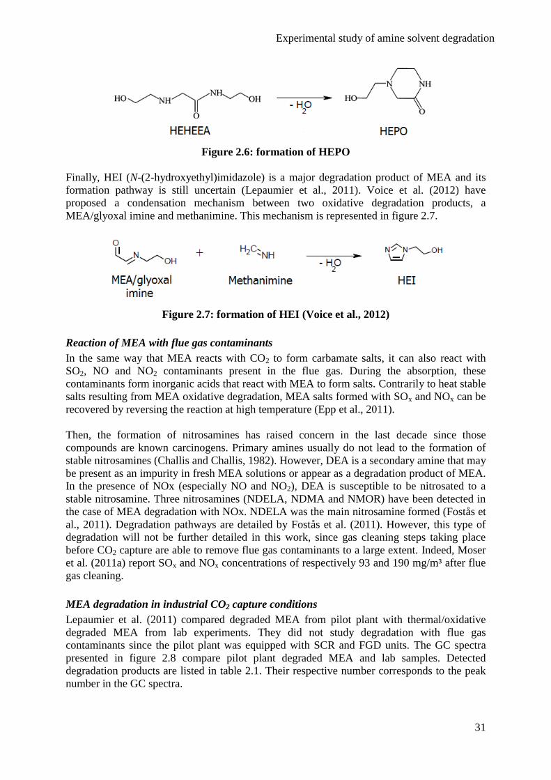
Figure 2.6: formation of HEPO

Finally, HEI (N-(2-hydroxyethyl)imidazole) is a major degradation product of MEA and its

formation pathway is still uncertain (Lepaumier et al., 2011). Voice et al. (2012) have

proposed a condensation mechanism between two oxidative degradation products, a

MEA/glyoxal imine and methanimine. This mechanism is represented in figure 2.7.

Figure 2.7: formation of HEI (Voice et al., 2012)

Reaction of MEA with flue gas contaminants

In the same way that MEA reacts with CO2 to form carbamate salts, it can also react with

SO2, NO and NO2 contaminants present in the flue gas. During the absorption, these

contaminants form inorganic acids that react with MEA to form salts. Contrarily to heat stable

salts resulting from MEA oxidative degradation, MEA salts formed with SOx and NOx can be

recovered by reversing the reaction at high temperature (Epp et al., 2011).

Then, the formation of nitrosamines has raised concern in the last decade since those

compounds are known carcinogens. Primary amines usually do not lead to the formation of

stable nitrosamines (Challis and Challis, 1982). However, DEA is a secondary amine that may

be present as an impurity in fresh MEA solutions or appear as a degradation product of MEA.

In the presence of NOx (especially NO and NO2), DEA is susceptible to be nitrosated to a

stable nitrosamine. Three nitrosamines (NDELA, NDMA and NMOR) have been detected in

the case of MEA degradation with NOx. NDELA was the main nitrosamine formed (Fostås et

al., 2011). Degradation pathways are detailed by Fostås et al. (2011). However, this type of

degradation will not be further detailed in this work, since gas cleaning steps taking place

before CO2 capture are able to remove flue gas contaminants to a large extent. Indeed, Moser

et al. (2011a) report SOx and NOx concentrations of respectively 93 and 190 mg/m³ after flue

gas cleaning.

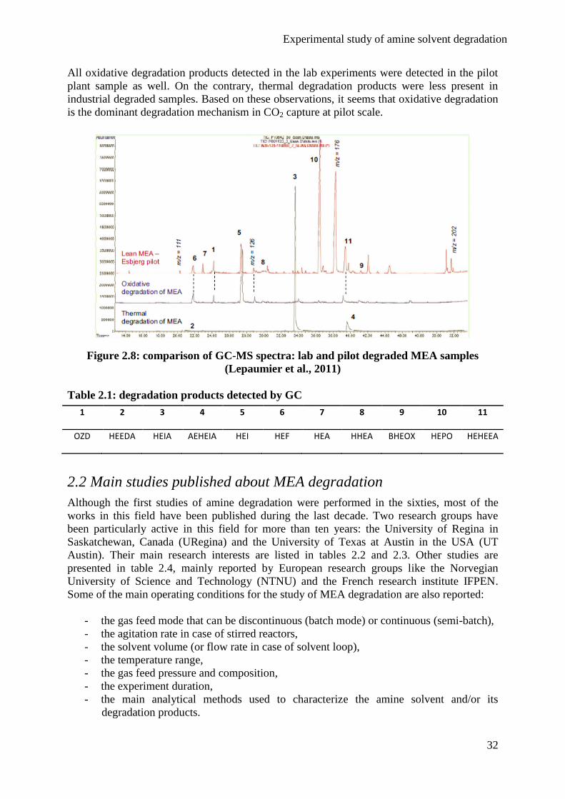
MEA degradation in industrial CO2 capture conditions

Lepaumier et al. (2011) compared degraded MEA from pilot plant with thermal/oxidative

degraded MEA from lab experiments. They did not study degradation with flue gas

contaminants since the pilot plant was equipped with SCR and FGD units. The GC spectra

presented in figure 2.8 compare pilot plant degraded MEA and lab samples. Detected

degradation products are listed in table 2.1. Their respective number corresponds to the peak

number in the GC spectra.

Experimental study of amine solvent degradation

32

All oxidative degradation products detected in the lab experiments were detected in the pilot

plant sample as well. On the contrary, thermal degradation products were less present in

industrial degraded samples. Based on these observations, it seems that oxidative degradation

is the dominant degradation mechanism in CO2 capture at pilot scale.

Figure 2.8: comparison of GC-MS spectra: lab and pilot degraded MEA samples

(Lepaumier et al., 2011)

Table 2.1: degradation products detected by GC

1 2 3 4 5 6 7 8 9 10 11

OZD HEEDA HEIA AEHEIA HEI HEF HEA HHEA BHEOX HEPO HEHEEA

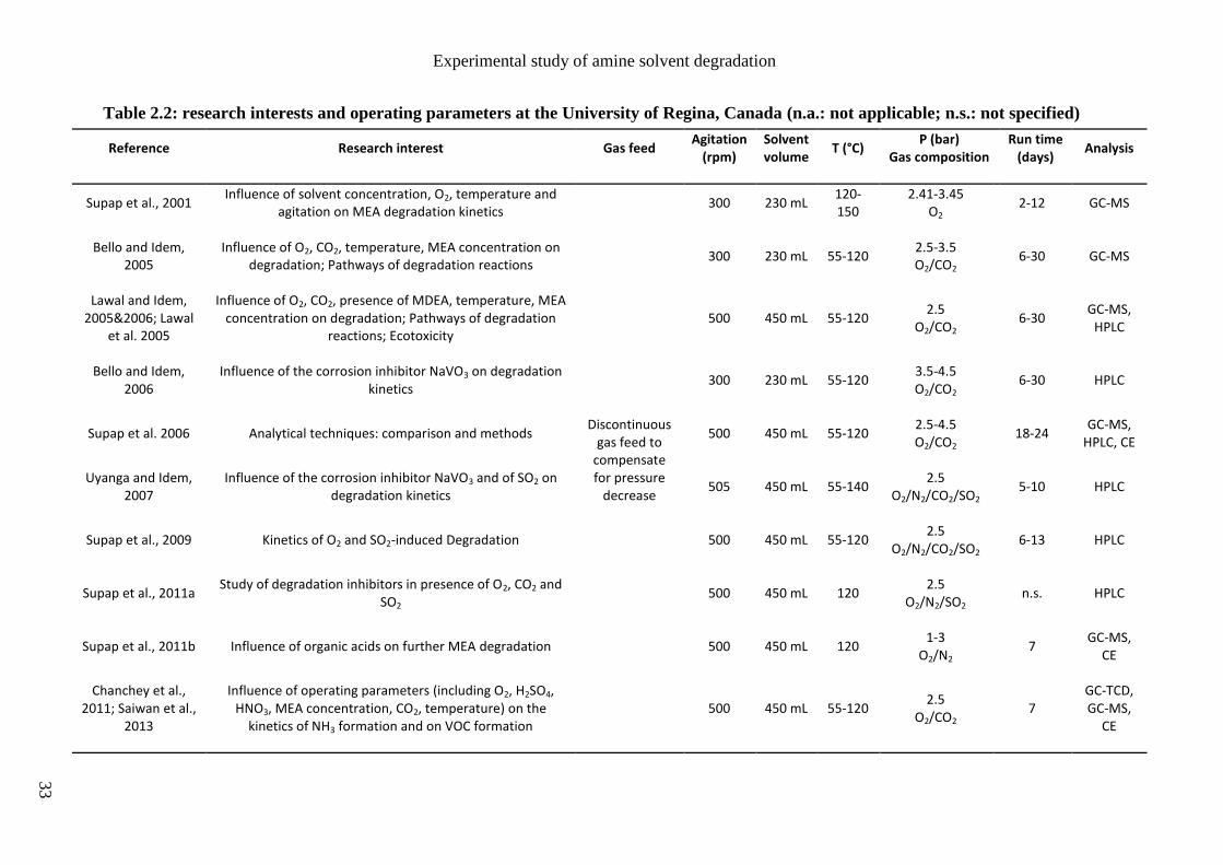
2.2 Main studies published about MEA degradation

Although the first studies of amine degradation were performed in the sixties, most of the

works in this field have been published during the last decade. Two research groups have

been particularly active in this field for more than ten years: the University of Regina in

Saskatchewan, Canada (URegina) and the University of Texas at Austin in the USA (UT

Austin). Their main research interests are listed in tables 2.2 and 2.3. Other studies are

presented in table 2.4, mainly reported by European research groups like the Norvegian

University of Science and Technology (NTNU) and the French research institute IFPEN.

Some of the main operating conditions for the study of MEA degradation are also reported:

- the gas feed mode that can be discontinuous (batch mode) or continuous (semi-batch),

- the agitation rate in case of stirred reactors,

- the solvent volume (or flow rate in case of solvent loop),

- the temperature range,

- the gas feed pressure and composition,

- the experiment duration,

- the main analytical methods used to characterize the amine solvent and/or its

degradation products.

Experimental study of amine solvent degradation

33

Table 2.2: research interests and operating parameters at the University of Regina, Canada (n.a.: not applicable; n.s.: not specified)

Reference Research interest Gas feed Agitation

(rpm) Solvent volume

T (°C) P (bar)

Gas composition Run time

(days) Analysis

Supap et al., 2001 Influence of solvent concentration, O2, temperature and

agitation on MEA degradation kinetics

Discontinuous gas feed to

compensate for pressure

decrease

300 230 mL 120-150

2.41-3.45 O2

2-12 GC-MS

Bello and Idem, 2005

Influence of O2, CO2, temperature, MEA concentration on degradation; Pathways of degradation reactions

300 230 mL 55-120 2.5-3.5 O2/CO2

6-30 GC-MS

Lawal and Idem, 2005&2006; Lawal

et al. 2005

Influence of O2, CO2, presence of MDEA, temperature, MEA concentration on degradation; Pathways of degradation

reactions; Ecotoxicity 500 450 mL 55-120

2.5 O2/CO2

6-30 GC-MS,

HPLC

Bello and Idem, 2006

Influence of the corrosion inhibitor NaVO3 on degradation kinetics

300 230 mL 55-120 3.5-4.5 O2/CO2

6-30 HPLC

Supap et al. 2006 Analytical techniques: comparison and methods 500 450 mL 55-120 2.5-4.5 O2/CO2

18-24 GC-MS,

HPLC, CE

Uyanga and Idem, 2007

Influence of the corrosion inhibitor NaVO3 and of SO2 on degradation kinetics

505 450 mL 55-140 2.5

O2/N2/CO2/SO2 5-10 HPLC

Supap et al., 2009 Kinetics of O2 and SO2-induced Degradation 500 450 mL 55-120 2.5

O2/N2/CO2/SO2 6-13 HPLC

Supap et al., 2011a Study of degradation inhibitors in presence of O2, CO2 and

SO2 500 450 mL 120

2.5 O2/N2/SO2

n.s. HPLC

Supap et al., 2011b Influence of organic acids on further MEA degradation 500 450 mL 120 1-3

O2/N2 7

GC-MS, CE

Chanchey et al., 2011; Saiwan et al.,

2013

Influence of operating parameters (including O2, H2SO4, HNO3, MEA concentration, CO2, temperature) on the

kinetics of NH3 formation and on VOC formation 500 450 mL 55-120

2.5 O2/CO2

7 GC-TCD, GC-MS,

CE

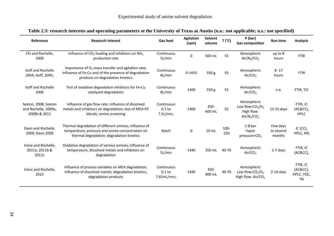
Experimental study of amine solvent degradation

34

Table 2.3: research interests and operating parameters at the University of Texas at Austin (n.a.: not applicable; n.s.: not specified)

Reference Research interest Gas feed Agitation

(rpm) Solvent volume

T (°C) P (bar)

Gas composition Run time Analysis

Chi and Rochelle, 2000

Influence of CO2-loading and inhibitors on NH3 production rate

Continuous 5L/min

0 500 mL 55 Atmospheric Air/N2/CO2

up to 8 hours

FTIR

Goff and Rochelle 2004; Goff, 2005;

Importance of O2-mass transfer and agitation rate; influence of Fe-Cu and of the presence of degradation

products on degradation kinetics

Continuous 8L/min

0-1450 550 g 55 Atmospheric

Air/CO2 8- 17 hours

FTIR

Goff and Rochelle 2006

Test of oxidative degradation inhibitors for Fe-Cu catalyzed degradation

Continuous 8L/min

1400 550 g 55 Atmospheric

Air/CO2 n.a. FTIR, TIC

Sexton, 2008; Sexton and Rochelle, 2009a,

2009b & 2011

Influence of gas flow rate; influence of dissolved metals and inhibitors on degradation; test of MEA-PZ

blends; amine screening

Continuous 0.1 to

7.5L/min; 1400

350- 400 mL

55

Atmospheric Low flow:CO2/O2

High flow: Air/N2/CO2

12-15 days FTIR, IC

(AC&CC), HPLC

Davis and Rochelle, 2009; Davis 2009

Thermal degradation of different amines; influence of temperature, pressure and amine concentration on

thermal degradation; degradation kinetics Batch 0 10 mL

100-150

1-8 bar Vapor

pressure+CO2

Few days to several months

IC (CC), HPLC, MS

Voice and Rochelle, 2011a, 2011b &

2011c

Oxidative degradation of various amines; influence of temperature, dissolved metals and inhibitors on

degradation

Continuous 5L/min

1440 350 mL 40-70 Atmospheric

Air/CO2 2-7 days

FTIR, IC (AC&CC),

Voice and Rochelle, 2013

Influence of process variables on MEA degradation; Influence of dissolved metals; degradation kinetics;

degradation products

Continuous 0.1 to

7.65mL/min; 1440

350-400 mL

40-70 Atmospheric

Low flow:CO2/O2

High flow: Air/CO2

2-14 days

FTIR, IC (AC&CC),

HPLC, TOC, TN

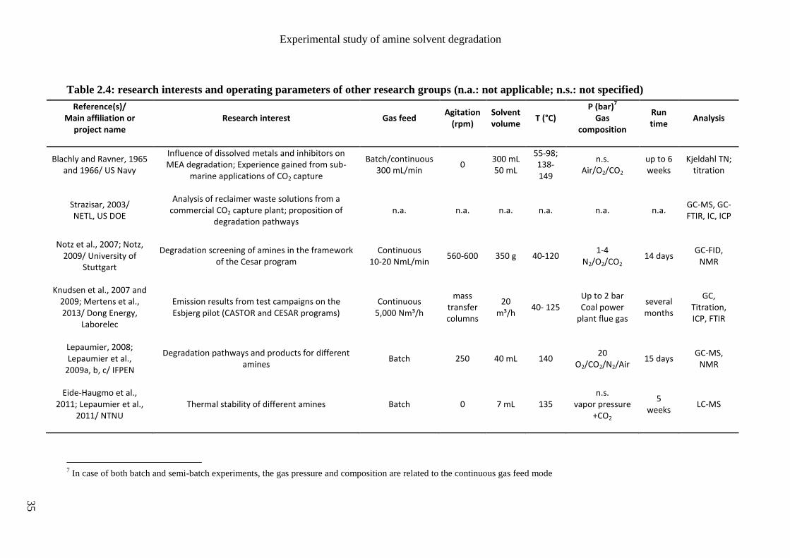
Experimental study of amine solvent degradation

35

Table 2.4: research interests and operating parameters of other research groups (n.a.: not applicable; n.s.: not specified)

Reference(s)/ Main affiliation or

project name Research interest Gas feed

Agitation (rpm)

Solvent volume

T (°C) P (bar)

7

Gas composition

Run time

Analysis

Blachly and Ravner, 1965 and 1966/ US Navy

Influence of dissolved metals and inhibitors on MEA degradation; Experience gained from sub-

marine applications of CO2 capture

Batch/continuous 300 mL/min

0 300 mL 50 mL

55-98; 138-149

n.s. Air/O2/CO2

up to 6 weeks

Kjeldahl TN; titration

Strazisar, 2003/ NETL, US DOE

Analysis of reclaimer waste solutions from a commercial CO2 capture plant; proposition of

degradation pathways n.a. n.a. n.a. n.a. n.a. n.a.

GC-MS, GC-FTIR, IC, ICP

Notz et al., 2007; Notz, 2009/ University of

Stuttgart

Degradation screening of amines in the framework of the Cesar program

Continuous 10-20 NmL/min

560-600 350 g 40-120 1-4

N2/O2/CO2 14 days

GC-FID, NMR

Knudsen et al., 2007 and 2009; Mertens et al., 2013/ Dong Energy,

Laborelec

Emission results from test campaigns on the Esbjerg pilot (CASTOR and CESAR programs)

Continuous 5,000 Nm³/h

mass transfer columns

20 m³/h

40- 125 Up to 2 bar Coal power

plant flue gas

several months

GC, Titration, ICP, FTIR

Lepaumier, 2008; Lepaumier et al.,

2009a, b, c/ IFPEN

Degradation pathways and products for different amines

Batch 250 40 mL 140 20

O2/CO2/N2/Air 15 days

GC-MS, NMR

Eide-Haugmo et al., 2011; Lepaumier et al.,

2011/ NTNU Thermal stability of different amines Batch 0 7 mL 135

n.s. vapor pressure

+CO2

5 weeks

LC-MS

7 In case of both batch and semi-batch experiments, the gas pressure and composition are related to the continuous gas feed mode

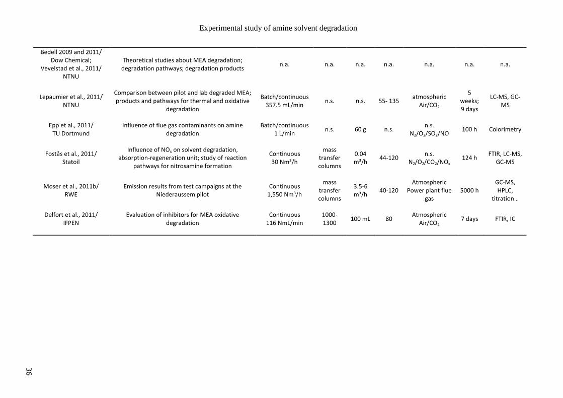
Experimental study of amine solvent degradation

36

Bedell 2009 and 2011/ Dow Chemical;

Vevelstad et al., 2011/ NTNU

Theoretical studies about MEA degradation; degradation pathways; degradation products

n.a. n.a. n.a. n.a. n.a. n.a. n.a.

Lepaumier et al., 2011/ NTNU

Comparison between pilot and lab degraded MEA; products and pathways for thermal and oxidative

degradation

Batch/continuous 357.5 mL/min

n.s. n.s. 55- 135 atmospheric

Air/CO2

5 weeks;9 days

LC-MS, GC-MS

Epp et al., 2011/ TU Dortmund

Influence of flue gas contaminants on amine degradation

Batch/continuous 1 L/min

n.s. 60 g n.s. n.s.

N2/O2/SO2/NO 100 h Colorimetry

Fostås et al., 2011/ Statoil

Influence of NOx on solvent degradation, absorption-regeneration unit; study of reaction

pathways for nitrosamine formation

Continuous 30 Nm³/h

mass transfer columns

0.04 m³/h

44-120 n.s.

N2/O2/CO2/NOx 124 h

FTIR, LC-MS, GC-MS

Moser et al., 2011b/ RWE

Emission results from test campaigns at the Niederaussem pilot

Continuous 1,550 Nm³/h

mass transfer columns

3.5-6 m³/h

40-120 Atmospheric

Power plant flue gas

5000 h GC-MS, HPLC,

titration…

Delfort et al., 2011/ IFPEN

Evaluation of inhibitors for MEA oxidative degradation

Continuous 116 NmL/min

1000-1300

100 mL 80 Atmospheric

Air/CO2 7 days FTIR, IC

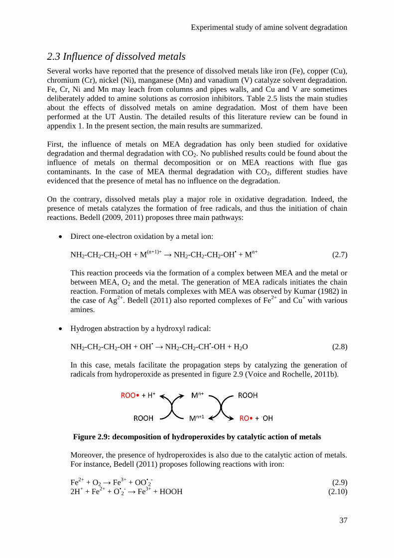
Experimental study of amine solvent degradation

37

2.3 Influence of dissolved metals

Several works have reported that the presence of dissolved metals like iron (Fe), copper (Cu),

chromium (Cr), nickel (Ni), manganese (Mn) and vanadium (V) catalyze solvent degradation.

Fe, Cr, Ni and Mn may leach from columns and pipes walls, and Cu and V are sometimes

deliberately added to amine solutions as corrosion inhibitors. Table 2.5 lists the main studies

about the effects of dissolved metals on amine degradation. Most of them have been

performed at the UT Austin. The detailed results of this literature review can be found in

appendix 1. In the present section, the main results are summarized.

First, the influence of metals on MEA degradation has only been studied for oxidative

degradation and thermal degradation with CO2. No published results could be found about the

influence of metals on thermal decomposition or on MEA reactions with flue gas

contaminants. In the case of MEA thermal degradation with CO2, different studies have

evidenced that the presence of metal has no influence on the degradation.

On the contrary, dissolved metals play a major role in oxidative degradation. Indeed, the

presence of metals catalyzes the formation of free radicals, and thus the initiation of chain

reactions. Bedell (2009, 2011) proposes three main pathways:

Direct one-electron oxidation by a metal ion:

NH2-CH2-CH2-OH + M(n+1)+

→ NH2-CH2-CH2-OH• + M

n+ (2.7)

This reaction proceeds via the formation of a complex between MEA and the metal or

between MEA, O2 and the metal. The generation of MEA radicals initiates the chain

reaction. Formation of metals complexes with MEA was observed by Kumar (1982) in

the case of Ag2+

. Bedell (2011) also reported complexes of Fe2+

and Cu+ with various

amines.

Hydrogen abstraction by a hydroxyl radical:

NH2-CH2-CH2-OH + OH• → NH2-CH2-CH

•-OH + H2O (2.8)

In this case, metals facilitate the propagation steps by catalyzing the generation of

radicals from hydroperoxide as presented in figure 2.9 (Voice and Rochelle, 2011b).

Figure 2.9: decomposition of hydroperoxides by catalytic action of metals

Moreover, the presence of hydroperoxides is also due to the catalytic action of metals.

For instance, Bedell (2011) proposes following reactions with iron:

Fe2+

+ O2 → Fe3+

+ OO•2-

(2.9)

2H+ + Fe

2+ + O

•2

- → Fe

3+ + HOOH (2.10)

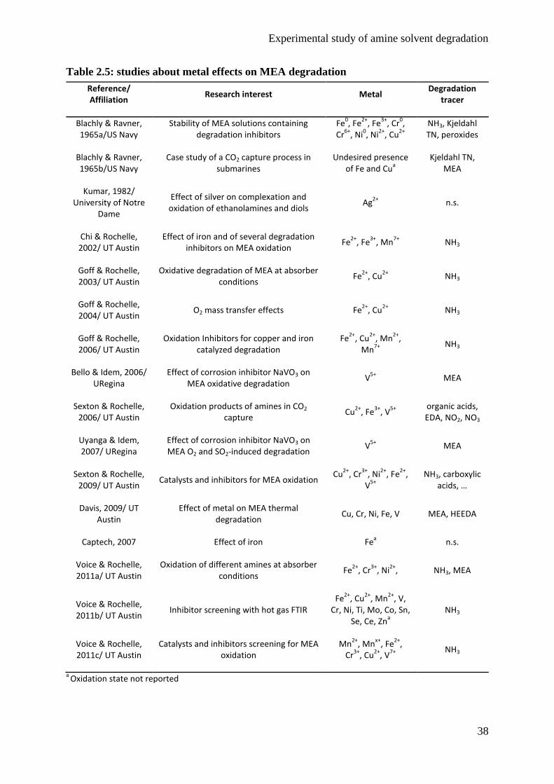
Experimental study of amine solvent degradation

38

Table 2.5: studies about metal effects on MEA degradation

Reference/ Affiliation

Research interest Metal Degradation

tracer

Blachly & Ravner, 1965a/US Navy

Stability of MEA solutions containing degradation inhibitors

Fe0, Fe

2+, Fe

3+, Cr

0,

Cr6+

, Ni0, Ni

2+, Cu

2+ NH3, Kjeldahl TN, peroxides

Blachly & Ravner, 1965b/US Navy

Case study of a CO2 capture process in submarines

Undesired presence of Fe and Cu

a Kjeldahl TN,

MEA

Kumar, 1982/ University of Notre

Dame

Effect of silver on complexation and oxidation of ethanolamines and diols

Ag2+

n.s.

Chi & Rochelle, 2002/ UT Austin

Effect of iron and of several degradation inhibitors on MEA oxidation

Fe2+

, Fe3+

, Mn7+

NH3

Goff & Rochelle, 2003/ UT Austin

Oxidative degradation of MEA at absorber conditions

Fe2+

, Cu2+

NH3

Goff & Rochelle, 2004/ UT Austin

O2 mass transfer effects Fe2+

, Cu2+

NH3

Goff & Rochelle, 2006/ UT Austin

Oxidation Inhibitors for copper and iron catalyzed degradation

Fe2+

, Cu2+

, Mn2+

, Mn

7+ NH3

Bello & Idem, 2006/ URegina

Effect of corrosion inhibitor NaVO3 on MEA oxidative degradation

V5+

MEA

Sexton & Rochelle, 2006/ UT Austin

Oxidation products of amines in CO2 capture

Cu2+

, Fe3+

, V5+ organic acids,

EDA, NO2, NO3

Uyanga & Idem, 2007/ URegina

Effect of corrosion inhibitor NaVO3 on MEA O2 and SO2-induced degradation

V5+

MEA

Sexton & Rochelle, 2009/ UT Austin

Catalysts and inhibitors for MEA oxidation Cu

2+, Cr

3+, Ni

2+, Fe

2+,

V5+

NH3, carboxylic acids, …

Davis, 2009/ UT Austin

Effect of metal on MEA thermal degradation

Cu, Cr, Ni, Fe, V

MEA, HEEDA

Captech, 2007 Effect of iron Fea n.s.

Voice & Rochelle, 2011a/ UT Austin

Oxidation of different amines at absorber conditions

Fe2+

, Cr3+

, Ni2+

, NH3, MEA

Voice & Rochelle, 2011b/ UT Austin

Inhibitor screening with hot gas FTIR Fe

2+, Cu

2+, Mn

2+, V,

Cr, Ni, Ti, Mo, Co, Sn, Se, Ce, Zn

a NH3

Voice & Rochelle, 2011c/ UT Austin

Catalysts and inhibitors screening for MEA oxidation

Mn2+

, Mnx+

, Fe2+

, Cr

3+, Cu

2+, V

7+ NH3

a Oxidation state not reported

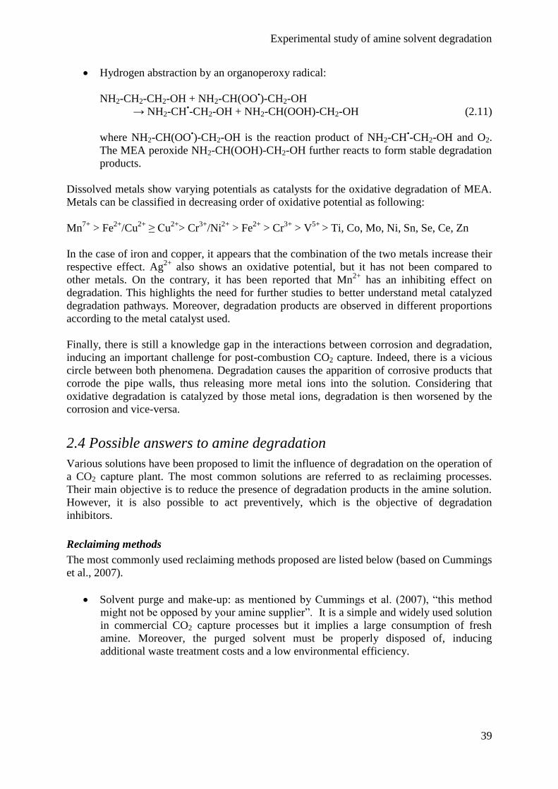
Experimental study of amine solvent degradation

39

Hydrogen abstraction by an organoperoxy radical:

NH2-CH2-CH2-OH + NH2-CH(OO•)-CH2-OH

→ NH2-CH•-CH2-OH + NH2-CH(OOH)-CH2-OH (2.11)

where NH2-CH(OO•)-CH2-OH is the reaction product of NH2-CH

•-CH2-OH and O2.

The MEA peroxide NH2-CH(OOH)-CH2-OH further reacts to form stable degradation

products.

Dissolved metals show varying potentials as catalysts for the oxidative degradation of MEA.

Metals can be classified in decreasing order of oxidative potential as following:

Mn7+

> Fe2+

/Cu2+

≥ Cu2+

> Cr3+

/Ni2+

> Fe2+

> Cr3+

> V5+

> Ti, Co, Mo, Ni, Sn, Se, Ce, Zn

In the case of iron and copper, it appears that the combination of the two metals increase their

respective effect. Ag2+

also shows an oxidative potential, but it has not been compared to

other metals. On the contrary, it has been reported that Mn2+

has an inhibiting effect on

degradation. This highlights the need for further studies to better understand metal catalyzed

degradation pathways. Moreover, degradation products are observed in different proportions

according to the metal catalyst used.

Finally, there is still a knowledge gap in the interactions between corrosion and degradation,

inducing an important challenge for post-combustion CO2 capture. Indeed, there is a vicious

circle between both phenomena. Degradation causes the apparition of corrosive products that

corrode the pipe walls, thus releasing more metal ions into the solution. Considering that

oxidative degradation is catalyzed by those metal ions, degradation is then worsened by the

corrosion and vice-versa.

2.4 Possible answers to amine degradation

Various solutions have been proposed to limit the influence of degradation on the operation of

a CO2 capture plant. The most common solutions are referred to as reclaiming processes.

Their main objective is to reduce the presence of degradation products in the amine solution.

However, it is also possible to act preventively, which is the objective of degradation

inhibitors.

Reclaiming methods

The most commonly used reclaiming methods proposed are listed below (based on Cummings

et al., 2007).

Solvent purge and make-up: as mentioned by Cummings et al. (2007), “this method

might not be opposed by your amine supplier”. It is a simple and widely used solution

in commercial CO2 capture processes but it implies a large consumption of fresh

amine. Moreover, the purged solvent must be properly disposed of, inducing

additional waste treatment costs and a low environmental efficiency.

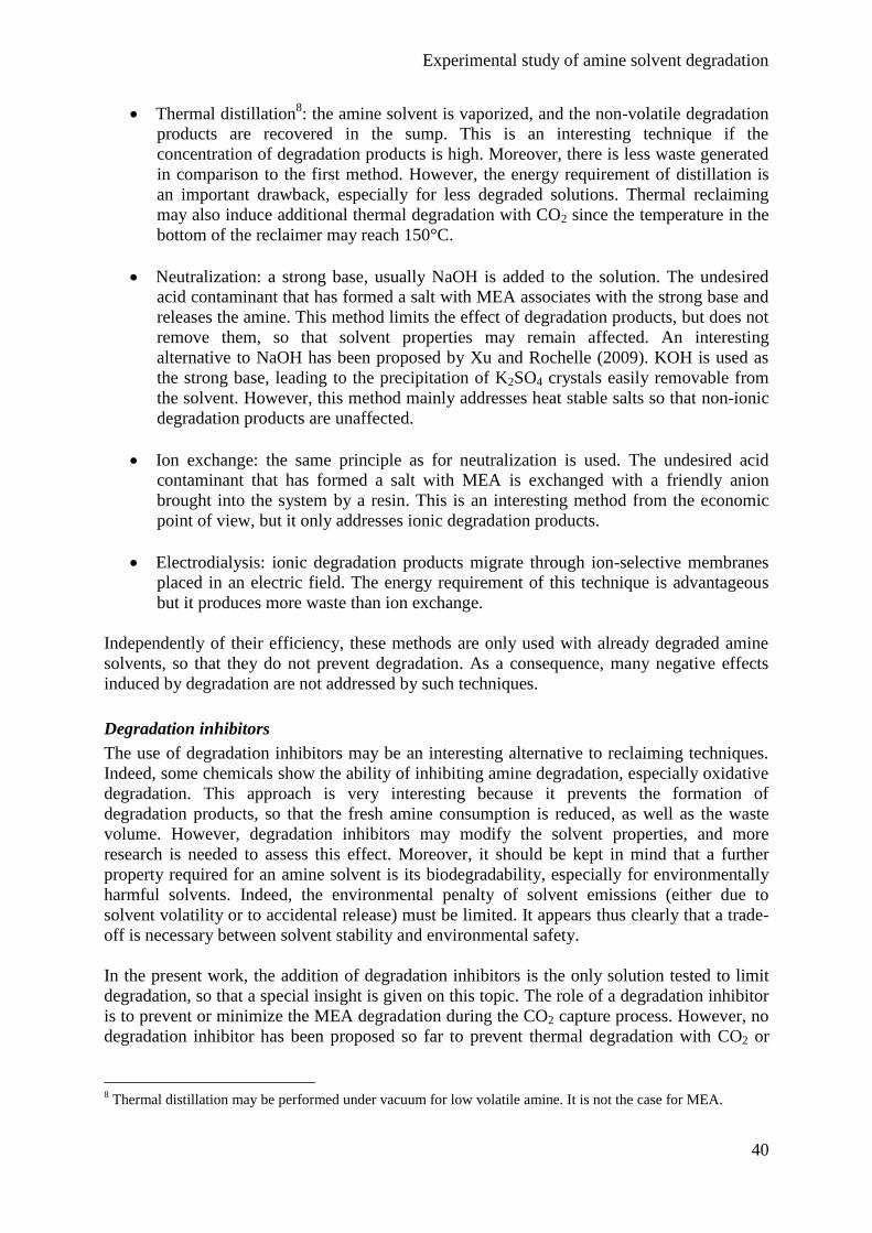
Experimental study of amine solvent degradation

40

Thermal distillation8: the amine solvent is vaporized, and the non-volatile degradation

products are recovered in the sump. This is an interesting technique if the

concentration of degradation products is high. Moreover, there is less waste generated

in comparison to the first method. However, the energy requirement of distillation is

an important drawback, especially for less degraded solutions. Thermal reclaiming

may also induce additional thermal degradation with CO2 since the temperature in the

bottom of the reclaimer may reach 150°C.

Neutralization: a strong base, usually NaOH is added to the solution. The undesired

acid contaminant that has formed a salt with MEA associates with the strong base and

releases the amine. This method limits the effect of degradation products, but does not

remove them, so that solvent properties may remain affected. An interesting

alternative to NaOH has been proposed by Xu and Rochelle (2009). KOH is used as

the strong base, leading to the precipitation of K2SO4 crystals easily removable from

the solvent. However, this method mainly addresses heat stable salts so that non-ionic

degradation products are unaffected.

Ion exchange: the same principle as for neutralization is used. The undesired acid

contaminant that has formed a salt with MEA is exchanged with a friendly anion

brought into the system by a resin. This is an interesting method from the economic

point of view, but it only addresses ionic degradation products.

Electrodialysis: ionic degradation products migrate through ion-selective membranes

placed in an electric field. The energy requirement of this technique is advantageous

but it produces more waste than ion exchange.

Independently of their efficiency, these methods are only used with already degraded amine

solvents, so that they do not prevent degradation. As a consequence, many negative effects

induced by degradation are not addressed by such techniques.

Degradation inhibitors

The use of degradation inhibitors may be an interesting alternative to reclaiming techniques.

Indeed, some chemicals show the ability of inhibiting amine degradation, especially oxidative

degradation. This approach is very interesting because it prevents the formation of

degradation products, so that the fresh amine consumption is reduced, as well as the waste

volume. However, degradation inhibitors may modify the solvent properties, and more

research is needed to assess this effect. Moreover, it should be kept in mind that a further

property required for an amine solvent is its biodegradability, especially for environmentally

harmful solvents. Indeed, the environmental penalty of solvent emissions (either due to

solvent volatility or to accidental release) must be limited. It appears thus clearly that a trade-

off is necessary between solvent stability and environmental safety.

In the present work, the addition of degradation inhibitors is the only solution tested to limit

degradation, so that a special insight is given on this topic. The role of a degradation inhibitor

is to prevent or minimize the MEA degradation during the CO2 capture process. However, no

degradation inhibitor has been proposed so far to prevent thermal degradation with CO2 or

8 Thermal distillation may be performed under vacuum for low volatile amine. It is not the case for MEA.

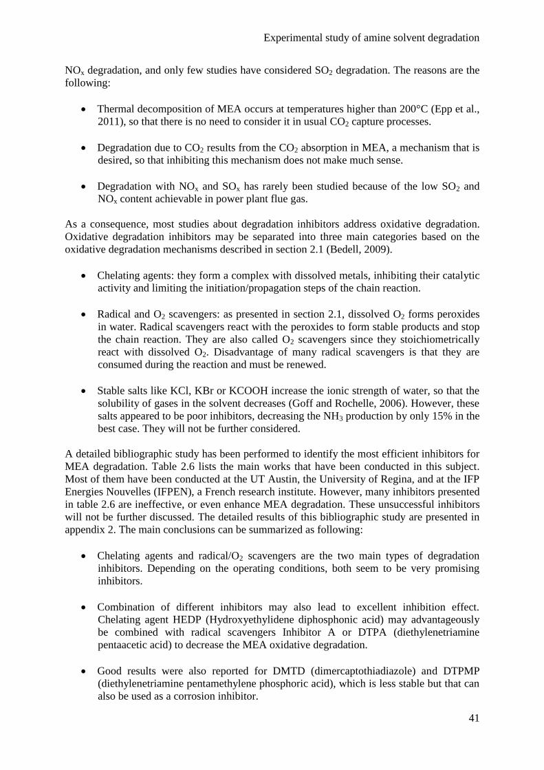
Experimental study of amine solvent degradation

41

NOx degradation, and only few studies have considered SO2 degradation. The reasons are the

following:

Thermal decomposition of MEA occurs at temperatures higher than 200°C (Epp et al.,

2011), so that there is no need to consider it in usual CO2 capture processes.

Degradation due to CO2 results from the CO2 absorption in MEA, a mechanism that is

desired, so that inhibiting this mechanism does not make much sense.

Degradation with NOx and SOx has rarely been studied because of the low SO2 and

NOx content achievable in power plant flue gas.

As a consequence, most studies about degradation inhibitors address oxidative degradation.

Oxidative degradation inhibitors may be separated into three main categories based on the

oxidative degradation mechanisms described in section 2.1 (Bedell, 2009).

Chelating agents: they form a complex with dissolved metals, inhibiting their catalytic

activity and limiting the initiation/propagation steps of the chain reaction.

Radical and O2 scavengers: as presented in section 2.1, dissolved O2 forms peroxides

in water. Radical scavengers react with the peroxides to form stable products and stop

the chain reaction. They are also called O2 scavengers since they stoichiometrically

react with dissolved O2. Disadvantage of many radical scavengers is that they are

consumed during the reaction and must be renewed.

Stable salts like KCl, KBr or KCOOH increase the ionic strength of water, so that the

solubility of gases in the solvent decreases (Goff and Rochelle, 2006). However, these

salts appeared to be poor inhibitors, decreasing the NH3 production by only 15% in the

best case. They will not be further considered.

A detailed bibliographic study has been performed to identify the most efficient inhibitors for

MEA degradation. Table 2.6 lists the main works that have been conducted in this subject.

Most of them have been conducted at the UT Austin, the University of Regina, and at the IFP

Energies Nouvelles (IFPEN), a French research institute. However, many inhibitors presented

in table 2.6 are ineffective, or even enhance MEA degradation. These unsuccessful inhibitors

will not be further discussed. The detailed results of this bibliographic study are presented in

appendix 2. The main conclusions can be summarized as following:

Chelating agents and radical/O2 scavengers are the two main types of degradation

inhibitors. Depending on the operating conditions, both seem to be very promising

inhibitors.

Combination of different inhibitors may also lead to excellent inhibition effect.

Chelating agent HEDP (Hydroxyethylidene diphosphonic acid) may advantageously

be combined with radical scavengers Inhibitor A or DTPA (diethylenetriamine

pentaacetic acid) to decrease the MEA oxidative degradation.

Good results were also reported for DMTD (dimercaptothiadiazole) and DTPMP

(diethylenetriamine pentamethylene phosphoric acid), which is less stable but that can

also be used as a corrosion inhibitor.

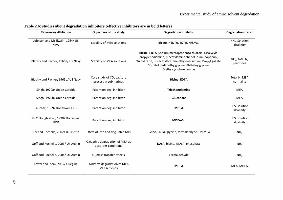
Experimental study of amine solvent degradation

42

Table 2.6: studies about degradation inhibitors (effective inhibitors are in bold letters)

Reference/ Affiliation Objectives of the study Degradation inhibitor Degradation tracer

Johnson and McElwain, 1964/ US Navy

Stability of MEA solutions Bicine, HEDTA, EDTA, NH4VO3 NH3, Solution

alcalinity

Blachly and Ravner, 1965a/ US Navy Stability of MEA solutions

Bicine, EDTA, Sodium mercaptobenzo thiazole, Disalycylal propylenediamine, p-acetylaminophenol, o-aminophenol,

Quinalizarin, bis-acetylacetene ethylenediimine, Propyl gallate, Sorbitol, n-dimethylglycine, Phthaloylglycine,

Diethylcyclohexylamine

NH3, total N, peroxides

Blachly and Ravner, 1965b/ US Navy Case study of CO2 capture

process in submarines Bicine, EDTA

Total N, MEA normality

Singh, 1970a/ Union Carbide Patent on deg. inhibitor Triethanolamine MEA

Singh, 1970b/ Union Carbide Patent on deg. inhibitor Gluconate MEA

Faucher, 1989/ Honeywell UOP Patent on deg. inhibitor MDEA HSS, solution

alcalinity

McCullough et al., 1990/ Honeywell UOP

Patent on deg. inhibitor MDEA-Sb HSS, solution

alcalinity

Chi and Rochelle, 2002/ UT Austin Effect of iron and deg. inhibitors Bicine, EDTA, glycine, formaldehyde, DMMEA NH3

Goff and Rochelle, 2003/ UT Austin Oxidative degradation of MEA at

absorber conditions EDTA, bicine, MDEA, phosphate NH3

Goff and Rochelle, 2004/ UT Austin O2 mass transfer effects Formaldehyde NH3

Lawal and Idem, 2005/ URegina Oxidative degradation of MEA-MDEA blends

MDEA MEA, MDEA

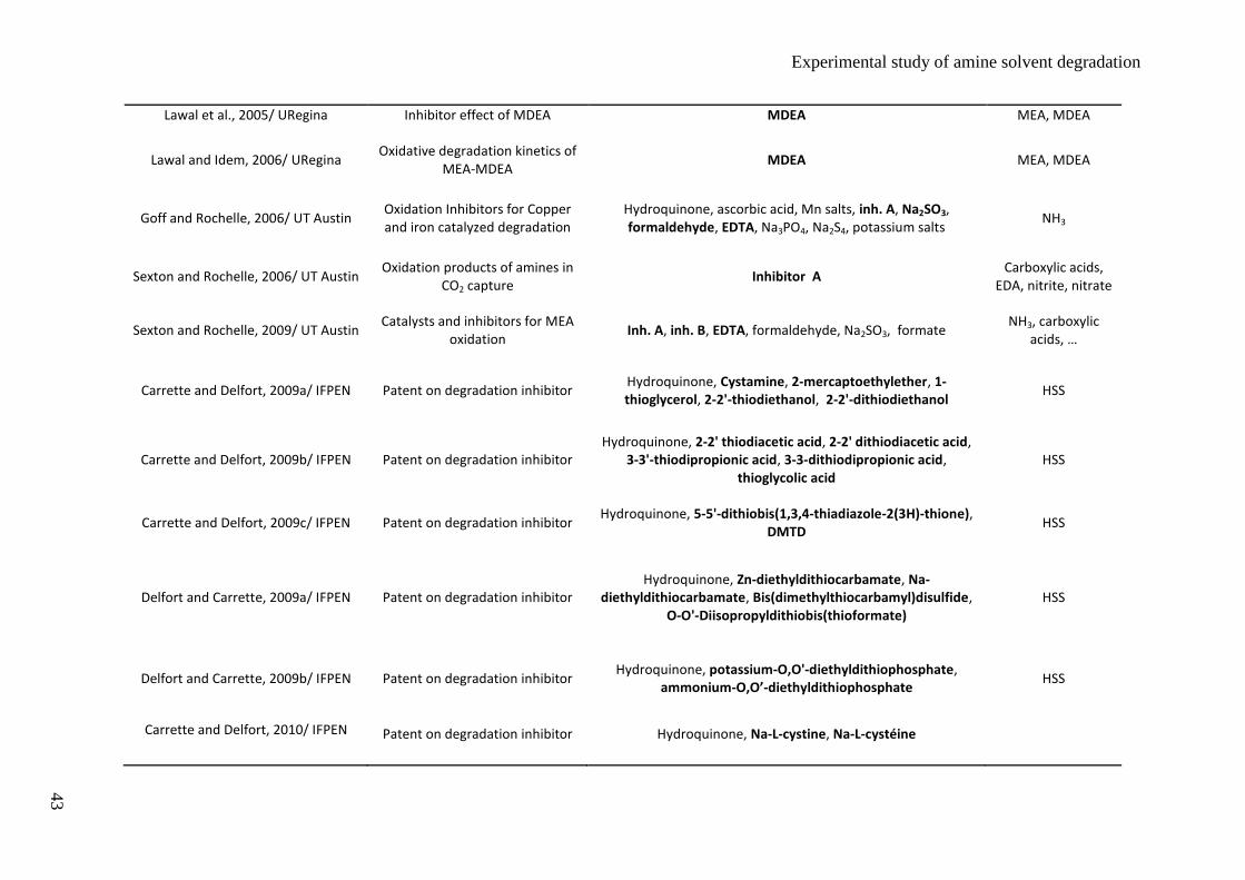
Experimental study of amine solvent degradation

Lawal et al., 2005/ URegina Inhibitor effect of MDEA MDEA MEA, MDEA

Lawal and Idem, 2006/ URegina Oxidative degradation kinetics of

MEA-MDEA MDEA MEA, MDEA

Goff and Rochelle, 2006/ UT Austin Oxidation Inhibitors for Copper and iron catalyzed degradation

Hydroquinone, ascorbic acid, Mn salts, inh. A, Na2SO3, formaldehyde, EDTA, Na3PO4, Na2S4, potassium salts

NH3

Sexton and Rochelle, 2006/ UT Austin Oxidation products of amines in

CO2 capture Inhibitor A

Carboxylic acids, EDA, nitrite, nitrate

Sexton and Rochelle, 2009/ UT Austin Catalysts and inhibitors for MEA

oxidation Inh. A, inh. B, EDTA, formaldehyde, Na2SO3, formate

NH3, carboxylic acids, …

Carrette and Delfort, 2009a/ IFPEN Patent on degradation inhibitor Hydroquinone, Cystamine, 2-mercaptoethylether, 1-thioglycerol, 2-2'-thiodiethanol, 2-2'-dithiodiethanol

HSS

Carrette and Delfort, 2009b/ IFPEN Patent on degradation inhibitor Hydroquinone, 2-2' thiodiacetic acid, 2-2' dithiodiacetic acid,

3-3'-thiodipropionic acid, 3-3-dithiodipropionic acid, thioglycolic acid

HSS

Carrette and Delfort, 2009c/ IFPEN Patent on degradation inhibitor Hydroquinone, 5-5'-dithiobis(1,3,4-thiadiazole-2(3H)-thione),

DMTD HSS

Delfort and Carrette, 2009a/ IFPEN Patent on degradation inhibitor Hydroquinone, Zn-diethyldithiocarbamate, Na-

diethyldithiocarbamate, Bis(dimethylthiocarbamyl)disulfide, O-O'-Diisopropyldithiobis(thioformate)

HSS

Delfort and Carrette, 2009b/ IFPEN Patent on degradation inhibitor Hydroquinone, potassium-O,O'-diethyldithiophosphate,

ammonium-O,O’-diethyldithiophosphate HSS

Carrette and Delfort, 2010/ IFPEN Patent on degradation inhibitor Hydroquinone, Na-L-cystine, Na-L-cystéine

43

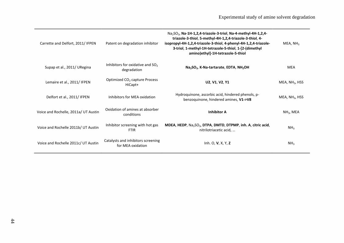
Experimental study of amine solvent degradation

44

Carrette and Delfort, 2011/ IFPEN Patent on degradation inhibitor

Na2SO3, Na-1H-1,2,4-triazole-3-triol, Na-4-methyl-4H-1,2,4-triazole-3-thiol, 5-methyl-4H-1,2,4-triazole-3-thiol, 4-

isopropyl-4H-1,2,4-triazole-3-thiol, 4-phenyl-4H-1,2,4-triazole-3-triol, 1-methyl-1H-tetrazole-5-thiol, 1-[2-(dimethyl

amino)ethyl]-1H-tetrazole-5-thiol

MEA, NH3

Supap et al., 2011/ URegina Inhibitors for oxidative and SO2

degradation Na2SO3, K-Na-tartarate, EDTA, NH2OH MEA

Lemaire et al., 2011/ IFPEN Optimized CO2 capture Process

HiCapt+ U2, V1, V2, Y1 MEA, NH3, HSS

Delfort et al., 2011/ IFPEN Inhibitors for MEA oxidation Hydroquinone, ascorbic acid, hindered phenols, p-

benzoquinone, hindered amines, V1->V8 MEA, NH3, HSS

Voice and Rochelle, 2011a/ UT Austin Oxidation of amines at absorber

conditions Inhibitor A NH3, MEA

Voice and Rochelle 2011b/ UT Austin Inhibitor screening with hot gas

FTIR MDEA, HEDP, Na2SO3, DTPA, DMTD, DTPMP, inh. A, citric acid,

nitrilotriacetic acid, … NH3

Voice and Rochelle 2011c/ UT Austin Catalysts and inhibitors screening

for MEA oxidation Inh. O, V, X, Y, Z NH3

Experimental study of amine solvent degradation

45

Finally, attention must also be paid at distinguishing degradation inhibitors from corrosion

inhibitors. Corrosion inhibitors like Cu and NaVO3 reduce the corrosive effect of the MEA

solution. However, they usually catalyze the oxidative degradation of MEA. On the contrary,

degradation inhibitors may contribute to a better solvent stability, but more research is needed

to assess their impact in pilot plant conditions and their influence on the solvent chemistry.

Experimental study of amine solvent degradation

46

3. Experimental methods

The experimental study of solvent degradation for CO2 capture was a new research field at the

University of Liège. This implied the development of an experimental test rig and procedures

that are presented in this section. First, the semi-batch degradation test rig where most

experiments were conducted is described. Then, the batch reactors used for the study of

thermal degradation under CO2 are also presented. Furthermore, it has been necessary to

develop in-house analytical methods to characterize degraded solvent solutions. Additional

analyses on degraded samples were also performed by other laboratories. These analytical

methods are also briefly described in this section.

3.1 Semi-batch degradation test rig

It has been evidenced that degradation takes place in industrial CO2 capture units. However,

degradation reactions show a slow kinetics. For instance, pilot scale tests during the CASTOR

project showed a decrease of the amine concentration by 4% in 45 days (Lepaumier, 2008).

For practical reasons, it is necessary to accelerate degradation in order to get experimental

data within a reasonable timeframe. However, experimental conditions should also remain as

representative as possible of the real CO2 capture conditions, so that degradation mechanisms

are similar.

The degradation test rig (DTR) developed at the University of Liège is represented in figure

2.10. During the design process, a special attention has been paid to enable flexible operating

conditions. The test rig is composed of five main parts:

1. Degradation reactor

2. Gas supply

3. Water balance control: gas saturator (3a) and condenser (3b)

4. Gas outlet and analysis

5. Data acquisition and control panel

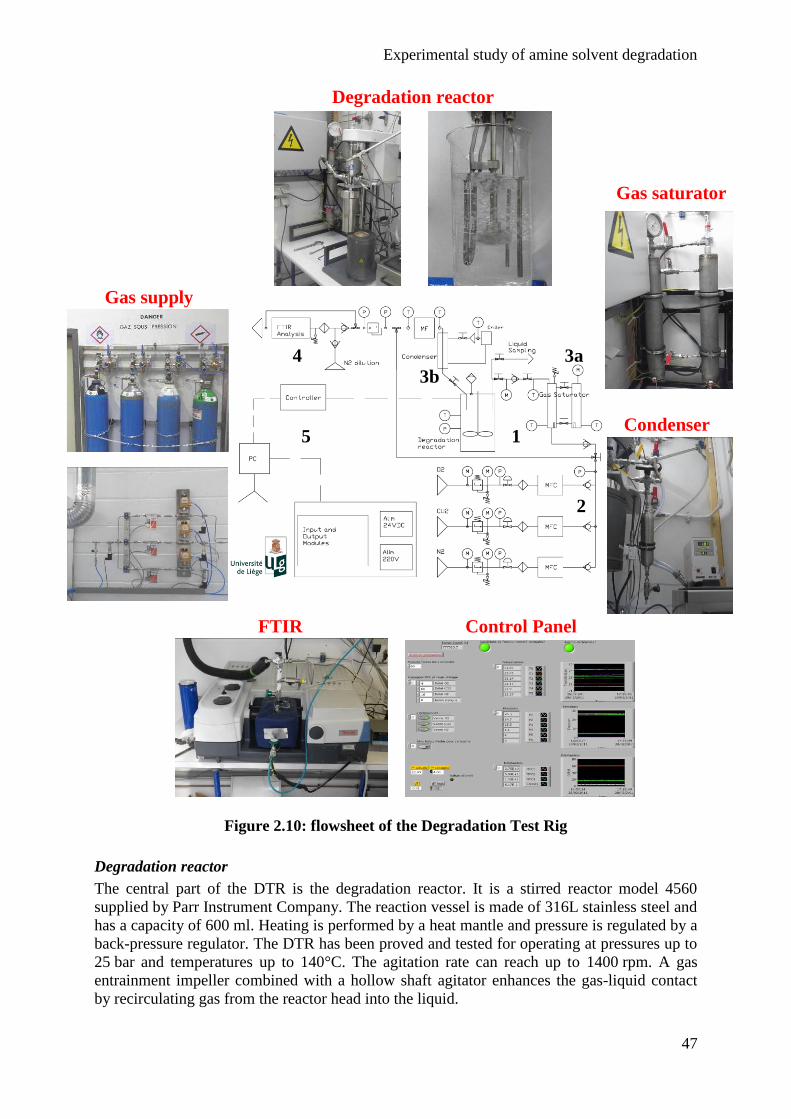
Experimental study of amine solvent degradation

47

Condenser

Figure 2.10: flowsheet of the Degradation Test Rig

Degradation reactor

The central part of the DTR is the degradation reactor. It is a stirred reactor model 4560

supplied by Parr Instrument Company. The reaction vessel is made of 316L stainless steel and

has a capacity of 600 ml. Heating is performed by a heat mantle and pressure is regulated by a

back-pressure regulator. The DTR has been proved and tested for operating at pressures up to

25 bar and temperatures up to 140°C. The agitation rate can reach up to 1400 rpm. A gas

entrainment impeller combined with a hollow shaft agitator enhances the gas-liquid contact

by recirculating gas from the reactor head into the liquid.

2

1

3a 4

5

3b

Degradation reactor

Gas supply

Gas saturator

FTIR Control Panel

Experimental study of amine solvent degradation

48

Gas supply

The DTR can be operated in batch or semi-batch mode depending on the gas feed mode

(continuous gas flow or not)9. The gas feed is composed by mixing up to three different gases,

usually O2, CO2 and N2. The proportion of each gas can vary between 0 and 100%. The total

gas flow rate can reach up to 1590 ml/min in normal conditions (0°C and 1 bar).

Water balance control

Because degradation experiments last for several days with continuous gas flow, it is

important to pay attention at the water balance. Before entering the degradation reactor, the

gas is saturated with water. Then, the gas exiting the reactor flows through a condenser where

it is cooled down while the condensed water is recycled to the reactor. Without this

equipment, the entering dry flue gas would get loaded with water in the reactor and would

quickly remove water from the system.

Gas outlet and analysis

The exhaust gas can be analyzed in an on-line FTIR analyzer before being released to the

atmosphere. To prevent gas condensation in the pipes, the line between the back-pressure

regulator and the FTIR analyzer is heated at 150°C. Moreover, the gas is diluted with hot

nitrogen to facilitate the FTIR analysis.

Data acquisition and control panel

Two control systems are combined to operate the DTR. First, the temperature and agitation

rate of the reactor are controlled by a dedicated controller provided with the reactor. Measured

data are recorded by a computer. Then, other experimental parameters (other temperatures,

pressures, mass flows) are acquired and controlled using a Labview®

application.

Experimental protocol

First, 300 g of 30 wt% MEA solution is loaded into the reaction vessel. The solution is loaded

with CO2 until the pressure starts increasing, which means that the CO2 is not absorbed

anymore10

. The solution loading lasts for approximately one hour at 390 Nml/min CO2 and

400 rpm. The solution is then weighted and a 1.5 ml sample is taken. The experiment starts

when the heating it switched on. In order to control the water balance, the water temperature

in the gas saturator is kept constant at 35°C. The temperature of cooling water for the

condenser is regulated at 16.5°C11

. Gas analysis occurs online using the FTIR analyzer.

Liquid analysis does not occur on-line but a sampling port in the reactor head allows for

liquid sampling during the experiment. Liquid samples are immediately cooled down and kept

refrigerated to avoid further degradation. The experiments last for one or two weeks. At the

end of the experiment, a liquid sample is collected. Then, the solution is cooled down to

ambient temperature and degassed. It is weighted and stored at low temperature (~4°C).

A risk analysis about operating the DTR has been performed before the operation start. The

results of this analysis are reported in appendix 3.

9 On the liquid side, the DTR is always operated in batch mode.

10 In case of experiments with no CO2 in the flue gas, there is no previous CO2 loading.

11 The temperature difference between the saturator and the condenser is due to the pressure drop in the reactor

that leads to a lower specific humidity of the saturated gas in the condenser.

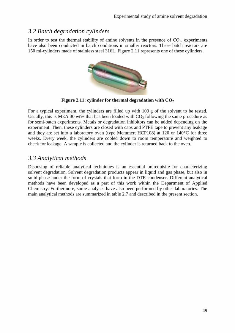
Experimental study of amine solvent degradation

49

3.2 Batch degradation cylinders

In order to test the thermal stability of amine solvents in the presence of CO2, experiments

have also been conducted in batch conditions in smaller reactors. These batch reactors are

150 ml-cylinders made of stainless steel 316L. Figure 2.11 represents one of these cylinders.

Figure 2.11: cylinder for thermal degradation with CO2

For a typical experiment, the cylinders are filled up with 100 g of the solvent to be tested.

Usually, this is MEA 30 wt% that has been loaded with CO2 following the same procedure as

for semi-batch experiments. Metals or degradation inhibitors can be added depending on the

experiment. Then, these cylinders are closed with caps and PTFE tape to prevent any leakage

and they are set into a laboratory oven (type Memmert HCP108) at 120 or 140°C for three

weeks. Every week, the cylinders are cooled down to room temperature and weighted to

check for leakage. A sample is collected and the cylinder is returned back to the oven.

3.3 Analytical methods

Disposing of reliable analytical techniques is an essential prerequisite for characterizing

solvent degradation. Solvent degradation products appear in liquid and gas phase, but also in

solid phase under the form of crystals that form in the DTR condenser. Different analytical

methods have been developed as a part of this work within the Department of Applied

Chemistry. Furthermore, some analyses have also been performed by other laboratories. The

main analytical methods are summarized in table 2.7 and described in the present section.

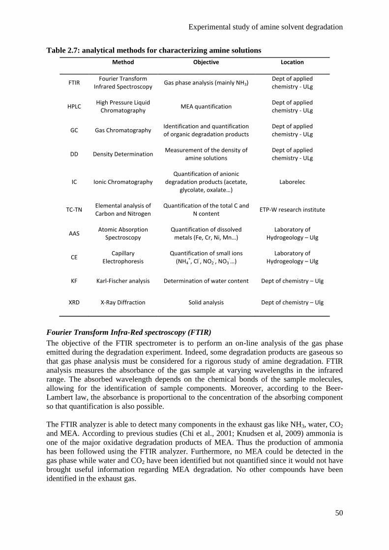
Experimental study of amine solvent degradation

50

Table 2.7: analytical methods for characterizing amine solutions

Method Objective Location

FTIR Fourier Transform

Infrared Spectroscopy Gas phase analysis (mainly NH3)

Dept of applied chemistry - ULg

HPLC High Pressure Liquid

Chromatography MEA quantification

Dept of applied chemistry - ULg

GC Gas Chromatography Identification and quantification of organic degradation products

Dept of applied chemistry - ULg

DD Density Determination Measurement of the density of

amine solutions Dept of applied chemistry - ULg

IC Ionic Chromatography Quantification of anionic

degradation products (acetate, glycolate, oxalate…)

Laborelec

TC-TN Elemental analysis of Carbon and Nitrogen

Quantification of the total C and N content

ETP-W research institute

AAS Atomic Absorption

Spectroscopy Quantification of dissolved

metals (Fe, Cr, Ni, Mn…) Laboratory of

Hydrogeology – Ulg

CE Capillary

Electrophoresis Quantification of small ions

(NH4+, Cl

-, NO2

-, NO3

-…)

Laboratory of Hydrogeology – Ulg

KF Karl-Fischer analysis Determination of water content Dept of chemistry – Ulg

XRD X-Ray Diffraction Solid analysis Dept of chemistry – Ulg

Fourier Transform Infra-Red spectroscopy (FTIR)

The objective of the FTIR spectrometer is to perform an on-line analysis of the gas phase

emitted during the degradation experiment. Indeed, some degradation products are gaseous so

that gas phase analysis must be considered for a rigorous study of amine degradation. FTIR

analysis measures the absorbance of the gas sample at varying wavelengths in the infrared

range. The absorbed wavelength depends on the chemical bonds of the sample molecules,

allowing for the identification of sample components. Moreover, according to the Beer-

Lambert law, the absorbance is proportional to the concentration of the absorbing component

so that quantification is also possible.

The FTIR analyzer is able to detect many components in the exhaust gas like NH3, water, CO2

and MEA. According to previous studies (Chi et al., 2001; Knudsen et al, 2009) ammonia is

one of the major oxidative degradation products of MEA. Thus the production of ammonia

has been followed using the FTIR analyzer. Furthermore, no MEA could be detected in the

gas phase while water and CO2 have been identified but not quantified since it would not have

brought useful information regarding MEA degradation. No other compounds have been

identified in the exhaust gas.

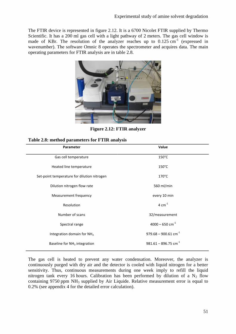
Experimental study of amine solvent degradation

51

The FTIR device is represented in figure 2.12. It is a 6700 Nicolet FTIR supplied by Thermo

Scientific. It has a 200 ml gas cell with a light pathway of 2 meters. The gas cell window is

made of KBr. The resolution of the analyzer reaches up to 0.125 cm-1

(expressed in

wavenumber). The software Omnic 8 operates the spectrometer and acquires data. The main

operating parameters for FTIR analysis are in table 2.8.

Figure 2.12: FTIR analyzer

Table 2.8: method parameters for FTIR analysis

Parameter Value

Gas cell temperature 150°C

Heated line temperature 150°C

Set-point temperature for dilution nitrogen 170°C

Dilution nitrogen flow rate 560 ml/min

Measurement frequency every 10 min

Resolution 4 cm-1

Number of scans 32/measurement

Spectral range 4000 – 650 cm-1

Integration domain for NH3 979.68 – 900.61 cm-1

Baseline for NH3 integration 981.61 – 896.75 cm-1

The gas cell is heated to prevent any water condensation. Moreover, the analyzer is

continuously purged with dry air and the detector is cooled with liquid nitrogen for a better

sensitivity. Thus, continuous measurements during one week imply to refill the liquid

nitrogen tank every 16 hours. Calibration has been performed by dilution of a N2 flow

containing 9750 ppm NH3 supplied by Air Liquide. Relative measurement error is equal to

0.2% (see appendix 4 for the detailed error calculation).

Experimental study of amine solvent degradation

52

Although the measurement error is very low, important perturbations may happen during on-

line FTIR monitoring, inducing some additional uncertainty on the NH3 production profile.

This problem is mainly due to the formation of crystals inside the condenser12

, which create a

solid plug and thus prevents the exhaust gas from exiting the condenser. This leads to a

pressure increase in the degradation reactor, triggering safety alarms that shut down the gas

supply. This may result in non-homogenous FTIR measurements.

The precipitation of crystals during amine degradation experiments was also reported by

several research groups (Tönnies, 2011; Lepaumier, 2011). However, this crystalline deposit

was not identified so far. Thermo-gravimetric differential scanning calorimetry (TG-DSC)

combined with mass spectrometry showed that the crystals start to decompose above 60°C

(figure 2.13), resulting in NH3, CO2 and water emission.

Figure 2.13: TG-DSC spectrum of a crystal sample

According to Meng (2004), the best identification method for ammonium salts is the X-Ray

Diffraction (XRD). Thus, the crystal has been analyzed by XRD at the Department of

Chemistry of the University of Liège. The observed spectrum corresponds perfectly with the

spectrum of ammonium carbonate (NH4HCO3) as shown in figure 2.14. Crystals of the same

type have been produced in almost all experiments with a gas feed containing O2 and CO2.

Finally, the precipitation of NH4HCO3 captures one mole of NH3 per mole of crystal,

inducing an error in the FTIR measurement of the NH3 production rate. As a consequence, the

production of NH3 (in mol) during degradation experiments was estimated as following:

(2.12)

12

A further problem was also recorded, probably due to foaming. Indeed, a large and sudden peak in the NH3

emission was sometimes detected by the FTIR. This was combined with a relative humidity of 100% at the gas

exhaust although the relative humidity of a saturated gas condensed at 4barg and 20°C should be equal to

19.98% at 1 barg and 20 °C. Foaming was suspected but could not be evidenced.

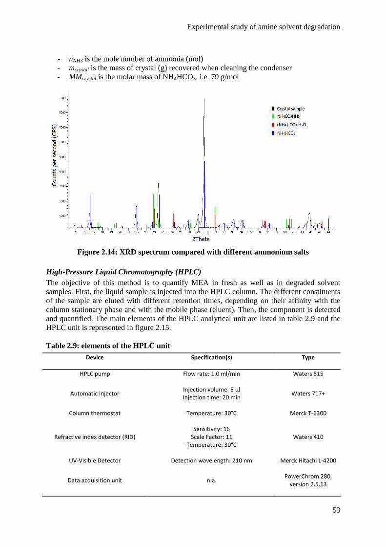
Experimental study of amine solvent degradation

53

- nNH3 is the mole number of ammonia (mol)

- mcrystal is the mass of crystal (g) recovered when cleaning the condenser

- MMcrystal is the molar mass of NH4HCO3, i.e. 79 g/mol

Figure 2.14: XRD spectrum compared with different ammonium salts

High-Pressure Liquid Chromatography (HPLC)

The objective of this method is to quantify MEA in fresh as well as in degraded solvent

samples. First, the liquid sample is injected into the HPLC column. The different constituents

of the sample are eluted with different retention times, depending on their affinity with the

column stationary phase and with the mobile phase (eluent). Then, the component is detected

and quantified. The main elements of the HPLC analytical unit are listed in table 2.9 and the

HPLC unit is represented in figure 2.15.

Table 2.9: elements of the HPLC unit

Device Specification(s) Type

HPLC pump Flow rate: 1.0 ml/min Waters 515

Automatic injector Injection volume: 5 µl Injection time: 20 min

Waters 717+

Column thermostat Temperature: 30°C Merck T-6300

Refractive index detector (RID) Sensitivity: 16

Scale Factor: 11 Temperature: 30°C

Waters 410

UV-Visible Detector Detection wavelength: 210 nm Merck Hitachi L-4200

Data acquisition unit n.a. PowerChrom 280,

version 2.5.13

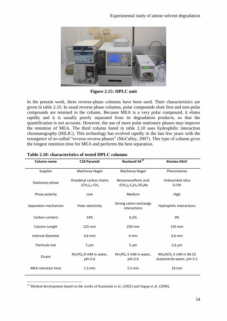
Experimental study of amine solvent degradation

54

Figure 2.15: HPLC unit

In the present work, three reverse-phase columns have been used. Their characteristics are

given in table 2.10. In usual reverse phase columns, polar compounds elute first and non-polar

compounds are retained in the column. Because MEA is a very polar compound, it elutes

rapidly and it is usually poorly separated from its degradation products, so that the

quantification is not accurate. However, the use of more polar stationary phases may improve

the retention of MEA. The third column listed in table 2.10 uses hydrophilic interaction

chromatography (HILIC). This technology has evolved rapidly in the last few years with the

resurgence of so-called “reverse-reverse phases” (McCalley, 2007). This type of column gives

the longest retention time for MEA and performs the best separation.

Table 2.10: characteristics of tested HPLC columns

Column name C18 Pyramid Nucleosil SA13

Kinetex HILIC

Supplier Macherey-Nagel Macherey-Nagel Phenomenex

Stationary phase Octadecyl carbon chains

-(CH2)17-CH3 Benzenesulfonic acid -(CH2)3-C6H4-SO3Na

Unbounded silica Si-OH

Phase polarity Low Medium High

Separation mechanism Polar selectivity Strong cation exchange

interactions Hydrophilic interactions

Carbon content 14% 6,5% 0%

Column Length 125 mm 250 mm 150 mm

Internal diameter 4,6 mm 4 mm 4,6 mm

Particule size 5 µm 5 µm 2,6 µm

Eluant KH2PO4 8 mM in water,

pH=2.6 KH2PO4 5 mM in water,

pH=2.6 NH4HCO2 5 mM in 90:10

Acetonitrile:water, pH=3.2

MEA retention time 1.5 min 5.5 min 16 min

13

Method development based on the works of Kaminski et al. (2002) and Supap et al. (2006).

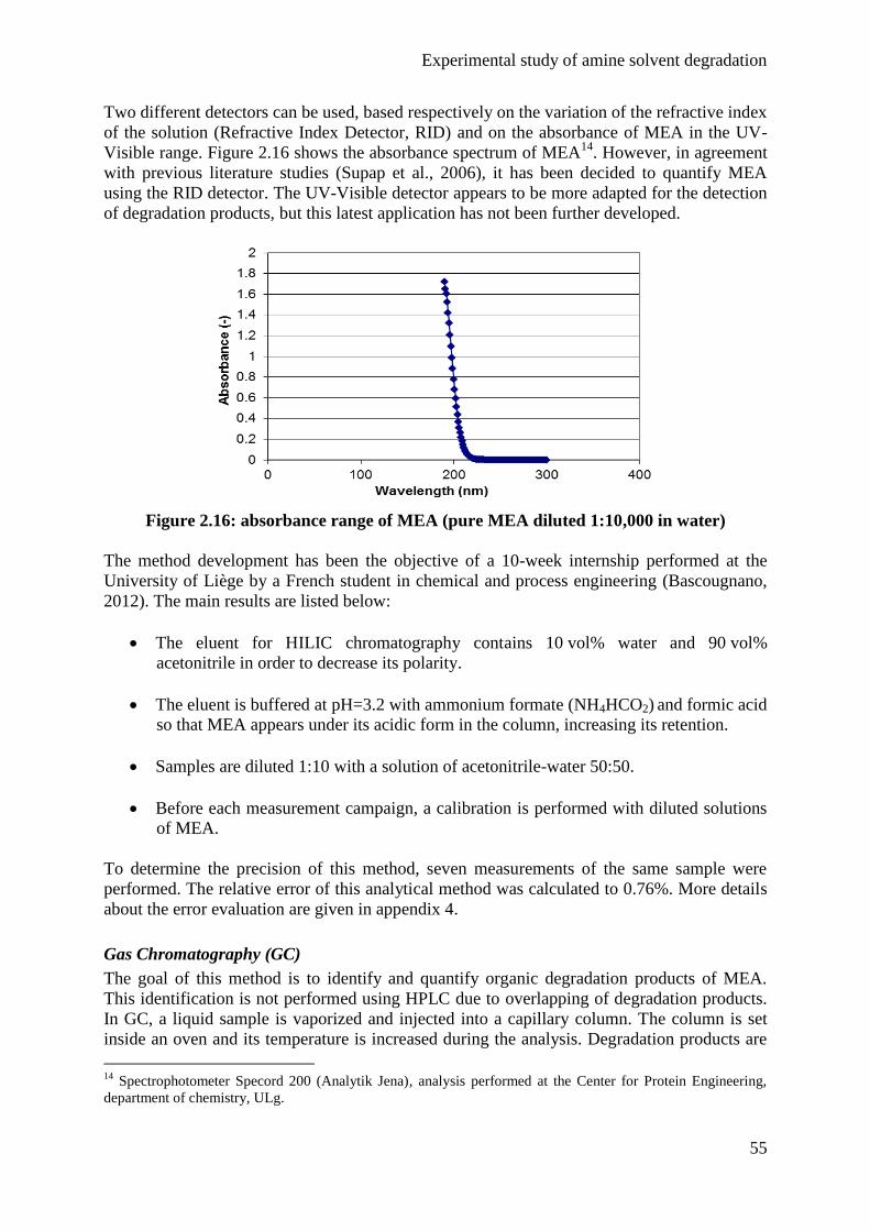
Experimental study of amine solvent degradation

55

Two different detectors can be used, based respectively on the variation of the refractive index

of the solution (Refractive Index Detector, RID) and on the absorbance of MEA in the UV-

Visible range. Figure 2.16 shows the absorbance spectrum of MEA14

. However, in agreement

with previous literature studies (Supap et al., 2006), it has been decided to quantify MEA

using the RID detector. The UV-Visible detector appears to be more adapted for the detection

of degradation products, but this latest application has not been further developed.

Figure 2.16: absorbance range of MEA (pure MEA diluted 1:10,000 in water)

The method development has been the objective of a 10-week internship performed at the

University of Liège by a French student in chemical and process engineering (Bascougnano,

2012). The main results are listed below:

The eluent for HILIC chromatography contains 10 vol% water and 90 vol%

acetonitrile in order to decrease its polarity.

The eluent is buffered at pH=3.2 with ammonium formate (NH4HCO2) and formic acid

so that MEA appears under its acidic form in the column, increasing its retention.

Samples are diluted 1:10 with a solution of acetonitrile-water 50:50.

Before each measurement campaign, a calibration is performed with diluted solutions

of MEA.

To determine the precision of this method, seven measurements of the same sample were

performed. The relative error of this analytical method was calculated to 0.76%. More details

about the error evaluation are given in appendix 4.

Gas Chromatography (GC)

The goal of this method is to identify and quantify organic degradation products of MEA.

This identification is not performed using HPLC due to overlapping of degradation products.

In GC, a liquid sample is vaporized and injected into a capillary column. The column is set

inside an oven and its temperature is increased during the analysis. Degradation products are

14

Spectrophotometer Specord 200 (Analytik Jena), analysis performed at the Center for Protein Engineering,

department of chemistry, ULg.

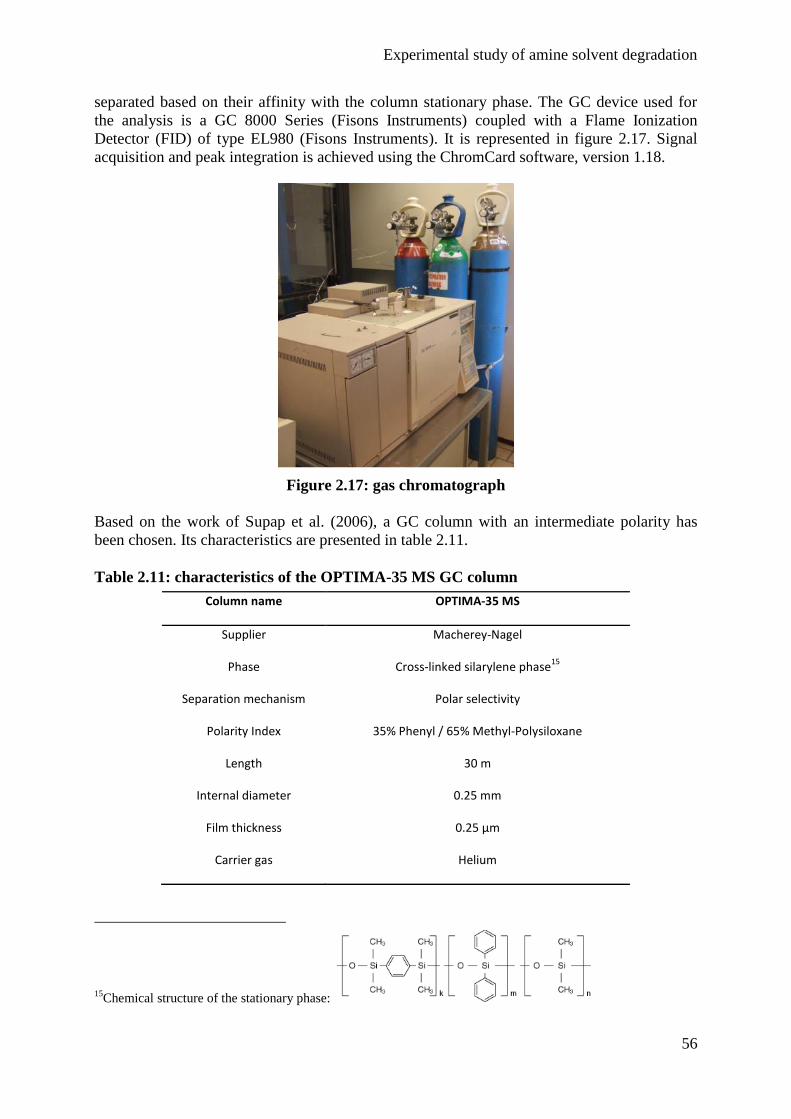
Experimental study of amine solvent degradation

56

separated based on their affinity with the column stationary phase. The GC device used for

the analysis is a GC 8000 Series (Fisons Instruments) coupled with a Flame Ionization

Detector (FID) of type EL980 (Fisons Instruments). It is represented in figure 2.17. Signal

acquisition and peak integration is achieved using the ChromCard software, version 1.18.

Figure 2.17: gas chromatograph

Based on the work of Supap et al. (2006), a GC column with an intermediate polarity has

been chosen. Its characteristics are presented in table 2.11.

Table 2.11: characteristics of the OPTIMA-35 MS GC column

Column name OPTIMA-35 MS

Supplier Macherey-Nagel

Phase Cross-linked silarylene phase15

Separation mechanism Polar selectivity

Polarity Index 35% Phenyl / 65% Methyl-Polysiloxane

Length 30 m

Internal diameter 0.25 mm

Film thickness 0.25 µm

Carrier gas Helium

15Chemical structure of the stationary phase:

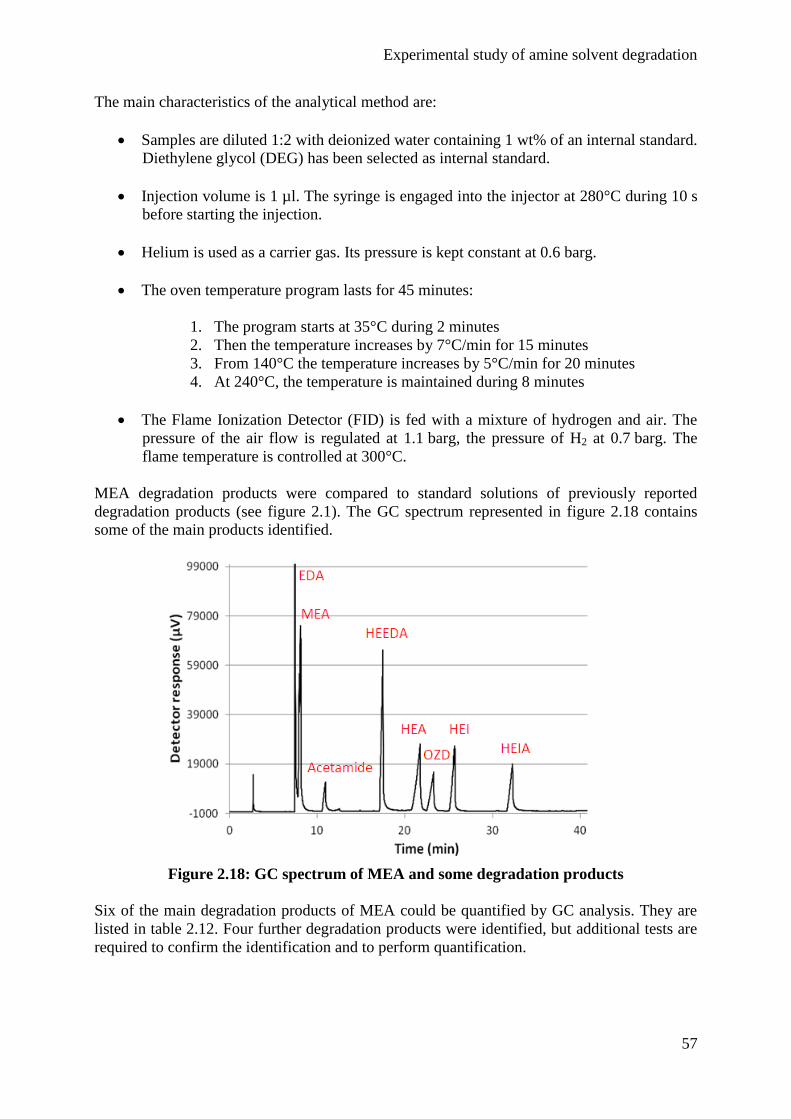
Experimental study of amine solvent degradation

57

The main characteristics of the analytical method are:

Samples are diluted 1:2 with deionized water containing 1 wt% of an internal standard.

Diethylene glycol (DEG) has been selected as internal standard.

Injection volume is 1 µl. The syringe is engaged into the injector at 280°C during 10 s

before starting the injection.

Helium is used as a carrier gas. Its pressure is kept constant at 0.6 barg.

The oven temperature program lasts for 45 minutes:

1. The program starts at 35°C during 2 minutes

2. Then the temperature increases by 7°C/min for 15 minutes

3. From 140°C the temperature increases by 5°C/min for 20 minutes

4. At 240°C, the temperature is maintained during 8 minutes

The Flame Ionization Detector (FID) is fed with a mixture of hydrogen and air. The

pressure of the air flow is regulated at 1.1 barg, the pressure of H2 at 0.7 barg. The

flame temperature is controlled at 300°C.

MEA degradation products were compared to standard solutions of previously reported

degradation products (see figure 2.1). The GC spectrum represented in figure 2.18 contains

some of the main products identified.

Figure 2.18: GC spectrum of MEA and some degradation products

Six of the main degradation products of MEA could be quantified by GC analysis. They are

listed in table 2.12. Four further degradation products were identified, but additional tests are

required to confirm the identification and to perform quantification.

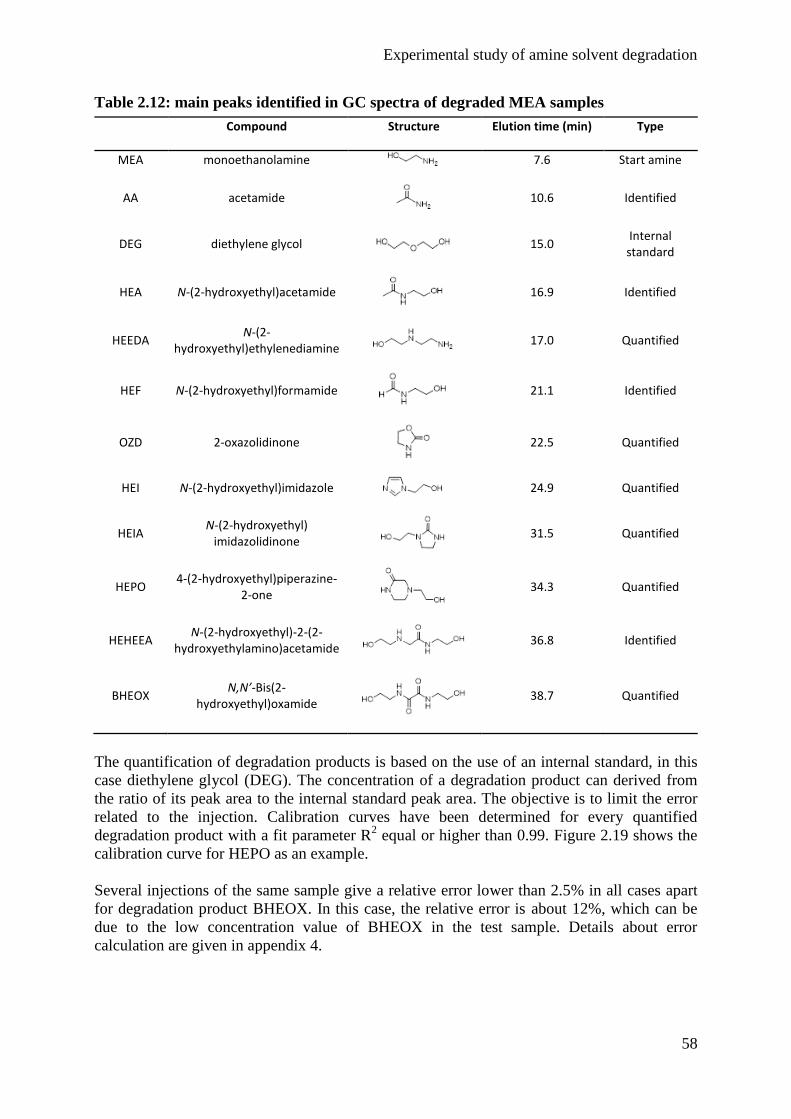
Experimental study of amine solvent degradation

58

Table 2.12: main peaks identified in GC spectra of degraded MEA samples

Compound Structure Elution time (min) Type

MEA monoethanolamine 7.6 Start amine

AA acetamide

10.6 Identified

DEG diethylene glycol 15.0 Internal standard

HEA N-(2-hydroxyethyl)acetamide

16.9 Identified

HEEDA N-(2-

hydroxyethyl)ethylenediamine 17.0 Quantified

HEF N-(2-hydroxyethyl)formamide

21.1 Identified

OZD 2-oxazolidinone

22.5 Quantified

HEI N-(2-hydroxyethyl)imidazole

24.9 Quantified

HEIA N-(2-hydroxyethyl)

imidazolidinone 31.5 Quantified

HEPO 4-(2-hydroxyethyl)piperazine-

2-one

34.3 Quantified

HEHEEA N-(2-hydroxyethyl)-2-(2-

hydroxyethylamino)acetamide 36.8 Identified

BHEOX N,N’-Bis(2-

hydroxyethyl)oxamide

38.7 Quantified

The quantification of degradation products is based on the use of an internal standard, in this

case diethylene glycol (DEG). The concentration of a degradation product can derived from

the ratio of its peak area to the internal standard peak area. The objective is to limit the error

related to the injection. Calibration curves have been determined for every quantified

degradation product with a fit parameter R2 equal or higher than 0.99. Figure 2.19 shows the

calibration curve for HEPO as an example.

Several injections of the same sample give a relative error lower than 2.5% in all cases apart

for degradation product BHEOX. In this case, the relative error is about 12%, which can be

due to the low concentration value of BHEOX in the test sample. Details about error

calculation are given in appendix 4.

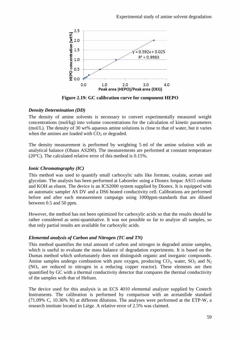
Experimental study of amine solvent degradation

59

Figure 2.19: GC calibration curve for component HEPO

Density Determination (DD)

The density of amine solvents is necessary to convert experimentally measured weight

concentrations (mol/kg) into volume concentrations for the calculation of kinetic parameters

(mol/L). The density of 30 wt% aqueous amine solutions is close to that of water, but it varies

when the amines are loaded with CO2 or degraded.

The density measurement is performed by weighting 5 ml of the amine solution with an

analytical balance (Ohaus AS200). The measurements are performed at constant temperature

(20°C). The calculated relative error of this method is 0.15%.

Ionic Chromatography (IC)

This method was used to quantify small carboxylic salts like formate, oxalate, acetate and

glycolate. The analysis has been performed at Laborelec using a Dionex Ionpac AS15 column

and KOH as eluent. The device is an ICS2000 system supplied by Dionex. It is equipped with

an automatic sampler AS DV and a DS6 heated conductivity cell. Calibrations are performed

before and after each measurement campaign using 1000ppm-standards that are diluted

between 0.5 and 50 ppm.

However, the method has not been optimized for carboxylic acids so that the results should be

rather considered as semi-quantitative. It was not possible so far to analyze all samples, so

that only partial results are available for carboxylic acids.

Elemental analysis of Carbon and Nitrogen (TC and TN)

This method quantifies the total amount of carbon and nitrogen in degraded amine samples,

which is useful to evaluate the mass balance of degradation experiments. It is based on the

Dumas method which unfortunately does not distinguish organic and inorganic compounds.

Amine samples undergo combustion with pure oxygen, producing CO2, water, SO2 and N2

(NOx are reduced to nitrogen in a reducing copper reactor). These elements are then

quantified by GC with a thermal conductivity detector that compares the thermal conductivity

of the samples with that of Helium.

The device used for this analysis is an ECS 4010 elemental analyzer supplied by Costech

Instruments. The calibration is performed by comparison with an acetanilide standard

(71.09% C, 10.36% N) at different dilutions. The analyses were performed at the ETP-W, a

research institute located in Liège. A relative error of 2.5% was claimed.

Experimental study of amine solvent degradation

60

Atomic absorption spectroscopy (AAS)

The concentration of dissolved metal was quantified by the Laboratory of Hydrogeology at

the University of Liège. The first objective of this method is to assess the qualitative evolution

of the corrosion in the degradation reactor. Indeed, the amount of dissolved metals is expected

to increase with more corrosive solutions and inversely, the presence of dissolved metals

catalyzes the oxidative degradation of amine solutions.

The degradation reactor is made of stainless steel 316L, so that the main metals that can leach

from the reactor vessel are Fe, Cr, Ni and Mn16

. Identification of metals in atomic absorption

spectroscopy is based on the absorption of specific wavelengths by metals. The Beer-Lambert

law is used to quantify the concentration of metals in the sample. Analyses were performed

using the flame spectrometer novAA®

300 supplied by Analytik Jena. Calibration tests were

performed with three solutions at 1.25, 2.5 and 6.5 mg/L for Fe, Cr, Ni and Mn. Prior to the

analysis, the amine sample was diluted with water and acidified with HCl or HNO3.

According to the operator, the relative standard deviations are usually below 10% for each

metal but they may reach up to 45% in case of low metal concentrations.

Capillary electrophoresis (CE)

This method was used to quantify some anionic and cationic degradation products like NH4+,

NO2-, NO3

-. Further anions like Cl

- and F

- were also analyzed due to their potential influence

on corrosion in the DTR. This analysis was performed at the Laboratory of Hydrogeology at

the University of Liège with a capillary ion analyzer 4000E supplied by Waters.

In capillary electrophoresis, the solution components are eluted along a capillary filled with

an electrolyte solution. The elution takes place under the influence of an electric field, so that

ions can be separated based on their size to charge ratio. Ions are detected by UV

spectrometry at 185 nm for cations and 254 nm for anions. Amine samples are diluted with

water, the dilution ratio depending on the sample conductivity. The quantification is

performed according an internal standard method. For cationic products, the internal standard

is Li+. For anionic products, it is ClO3

-. In the case of NH4

+ high uncertainties were reported

due to matrix perturbation. Indeed, carbonates are present in large amounts in loaded amine

samples and their peak may hide some other ions. Moreover, the measure of NH4+ may not be

relevant due to the high volatility of ammonia. As a consequence, values for NH4+ may rather

be considered as semi-quantitative.

Karl-Fischer titration of water (KF)

The Karl-Fischer analysis was performed by the Laboratory of Coordination and

Radiochemistry, part of the Department of Chemistry at the University of Liège. The

objective of this analysis is to determine the water content of amine solutions. This gives

some information about the water mass balance in the degradation reactor. The principle of

this method is a chemical titration based on the reaction of sulfur dioxide and iodine in the

presence of water:

2 H2O + SO2 + I2 → SO42−

+ 2 I− + 4 H

+ (2.13)

16

Silicon was also analyzed in some experiments because solution contamination due to a thread lubricant was

suspected. In this case, the concentrations of the calibration solutions were 50, 100 and 200mg/L.

Experimental study of amine solvent degradation

61

As long as water is available in the sample, it reacts with SO2 and iodine which is

progressively added to the sample. The titration end point is detected by potentiometry as

soon as I2 is in excess in the sample. Amine samples were diluted 1:20 with Ethanol. 100 µl

of the diluted solution have been titrated using an 831 KF Coulometer Metrohm apparatus.

The calibration was performed with aqueous solutions of MEA at concentrations of 12, 18,

24, 30 and 36 wt% MEA. The relative error of this method is lower than 1% (see appendix 4).

Experimental study of amine solvent degradation

62

4. Semi-batch experiments

Since the beginning of the first test campaign in March 2011, 13 two-week experiments and

23 one-week experiments have been conducted using the degradation test rig. In this section,

the main results of these 36 experiments are presented graphically and discussed. The detailed

figures can be found in appendix 5.

First, it was necessary to identify a base case for accelerated degradation in order to evaluate

the influence of different parameters. The relevance of this base case is evaluated by

comparing the results with degraded MEA samples from two different CO2 capture pilots.

Then, the influence of different process parameters is studied: O2 and CO2 content in the gas

feed, agitation rate, experiment length and temperature. The influence of dissolved metals and

degradation inhibitors is also studied. Finally, the repeatability of the results is evaluated, and

the error related to semi-batch degradation experiments is estimated.

4.1 Base case

The definition of a base case for accelerated degradation experiments is necessary to study the

influence of different operating parameters. The base case must present three main

characteristics:

Degradation must be observable

Degradation pathways must be similar to those occurring in CO2 capture plants

Parameter values must be in an intermediate range, so that they can be easily increased

or decreased

Different experiments have been performed to identify a suitable base case. Finally, the

conditions presented in table 2.13 have been selected.

Table 2.13: base case conditions for semi-batch degradation experiments

Parameter Value

Solvent 300 g of 30 wt% MEA loaded with CO2

(1.47 mol MEA)

Temperature 120°C

Pressure 4 barg

Agitation rate 600 rpm

Gas feed flow rate 160 Nml/min

Gas feed composition 5% O2 / 15% CO2 / 80% N2

Experiment duration 1 week

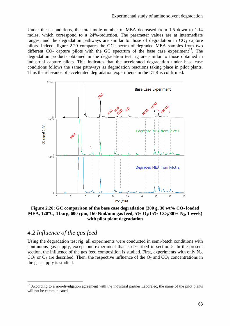
Experimental study of amine solvent degradation

63

Under these conditions, the total mole number of MEA decreased from 1.5 down to 1.14

moles, which correspond to a 24%-reduction. The parameter values are at intermediate

ranges, and the degradation pathways are similar to those of degradation in CO2 capture

pilots. Indeed, figure 2.20 compares the GC spectra of degraded MEA samples from two

different CO2 capture pilots with the GC spectrum of the base case experiment17

. The

degradation products obtained in the degradation test rig are similar to those obtained in

industrial capture pilots. This indicates that the accelerated degradation under base case

conditions follows the same pathways as degradation reactions taking place in pilot plants.

Thus the relevance of accelerated degradation experiments in the DTR is confirmed.

Figure 2.20: GC comparison of the base case degradation (300 g, 30 wt% CO2 loaded

MEA, 120°C, 4 barg, 600 rpm, 160 Nml/min gas feed, 5% O2/15% CO2/80% N2, 1 week)

with pilot plant degradation

4.2 Influence of the gas feed

Using the degradation test rig, all experiments were conducted in semi-batch conditions with

continuous gas supply, except one experiment that is described in section 5. In the present

section, the influence of the gas feed composition is studied. First, experiments with only N2,

CO2 or O2 are described. Then, the respective influence of the O2 and CO2 concentrations in

the gas supply is studied.

17

According to a non-divulgation agreement with the industrial partner Laborelec, the name of the pilot plants

will not be communicated.

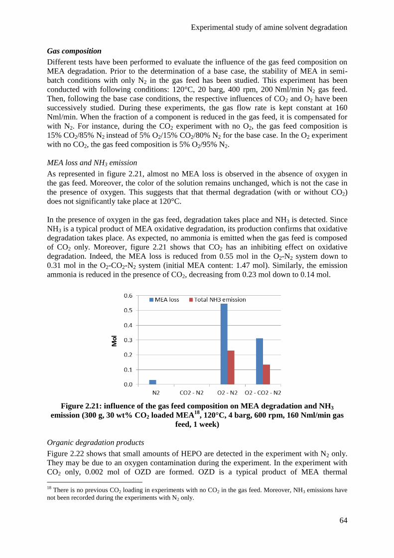
Experimental study of amine solvent degradation

64

Gas composition

Different tests have been performed to evaluate the influence of the gas feed composition on

MEA degradation. Prior to the determination of a base case, the stability of MEA in semi-

batch conditions with only N2 in the gas feed has been studied. This experiment has been

conducted with following conditions: 120°C, 20 barg, 400 rpm, 200 Nml/min N2 gas feed.

Then, following the base case conditions, the respective influences of CO2 and O2 have been

successively studied. During these experiments, the gas flow rate is kept constant at 160

Nml/min. When the fraction of a component is reduced in the gas feed, it is compensated for

with N2. For instance, during the CO2 experiment with no O2, the gas feed composition is

15% CO2/85% N2 instead of 5% O2/15% CO2/80% N2 for the base case. In the O2 experiment

with no CO2, the gas feed composition is 5% O2/95% N2.

MEA loss and NH3 emission

As represented in figure 2.21, almost no MEA loss is observed in the absence of oxygen in

the gas feed. Moreover, the color of the solution remains unchanged, which is not the case in

the presence of oxygen. This suggests that that thermal degradation (with or without CO2)

does not significantly take place at 120°C.

In the presence of oxygen in the gas feed, degradation takes place and NH3 is detected. Since

NH3 is a typical product of MEA oxidative degradation, its production confirms that oxidative

degradation takes place. As expected, no ammonia is emitted when the gas feed is composed

of CO2 only. Moreover, figure 2.21 shows that CO2 has an inhibiting effect on oxidative

degradation. Indeed, the MEA loss is reduced from 0.55 mol in the O2-N2 system down to

0.31 mol in the O2-CO2-N2 system (initial MEA content: 1.47 mol). Similarly, the emission

ammonia is reduced in the presence of CO2, decreasing from 0.23 mol down to 0.14 mol.

Figure 2.21: influence of the gas feed composition on MEA degradation and NH3

emission (300 g, 30 wt% CO2 loaded MEA18

, 120°C, 4 barg, 600 rpm, 160 Nml/min gas

feed, 1 week)

Organic degradation products

Figure 2.22 shows that small amounts of HEPO are detected in the experiment with N2 only.

They may be due to an oxygen contamination during the experiment. In the experiment with

CO2 only, 0.002 mol of OZD are formed. OZD is a typical product of MEA thermal

18

There is no previous CO2 loading in experiments with no CO2 in the gas feed. Moreover, NH3 emissions have

not been recorded during the experiments with N2 only.

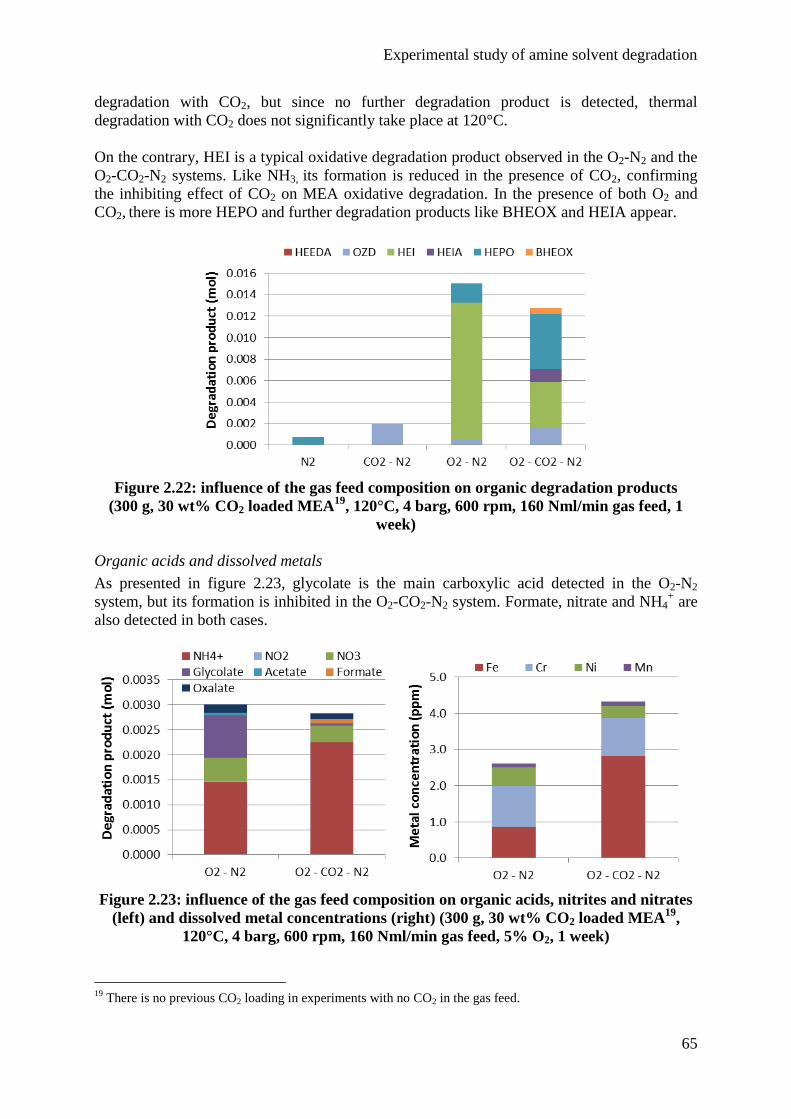
Experimental study of amine solvent degradation

65

degradation with CO2, but since no further degradation product is detected, thermal

degradation with CO2 does not significantly take place at 120°C.

On the contrary, HEI is a typical oxidative degradation product observed in the O2-N2 and the

O2-CO2-N2 systems. Like NH3, its formation is reduced in the presence of CO2, confirming

the inhibiting effect of CO2 on MEA oxidative degradation. In the presence of both O2 and

CO2, there is more HEPO and further degradation products like BHEOX and HEIA appear.

Figure 2.22: influence of the gas feed composition on organic degradation products

(300 g, 30 wt% CO2 loaded MEA19

, 120°C, 4 barg, 600 rpm, 160 Nml/min gas feed, 1

week)

Organic acids and dissolved metals

As presented in figure 2.23, glycolate is the main carboxylic acid detected in the O2-N2

system, but its formation is inhibited in the O2-CO2-N2 system. Formate, nitrate and NH4+ are

also detected in both cases.

Figure 2.23: influence of the gas feed composition on organic acids, nitrites and nitrates

(left) and dissolved metal concentrations (right) (300 g, 30 wt% CO2 loaded MEA19

,

120°C, 4 barg, 600 rpm, 160 Nml/min gas feed, 5% O2, 1 week)

19

There is no previous CO2 loading in experiments with no CO2 in the gas feed.

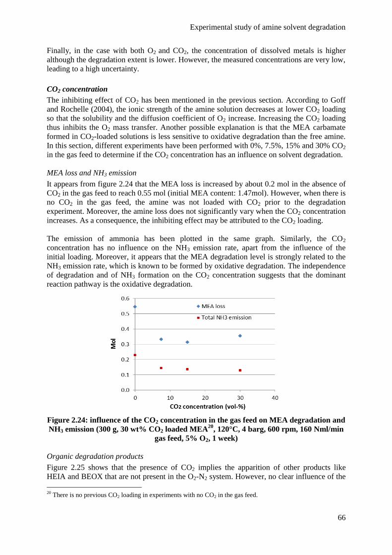
Experimental study of amine solvent degradation

66

Finally, in the case with both O2 and CO2, the concentration of dissolved metals is higher

although the degradation extent is lower. However, the measured concentrations are very low,

leading to a high uncertainty.

CO2 concentration

The inhibiting effect of CO2 has been mentioned in the previous section. According to Goff

and Rochelle (2004), the ionic strength of the amine solution decreases at lower CO2 loading

so that the solubility and the diffusion coefficient of O2 increase. Increasing the CO2 loading

thus inhibits the O2 mass transfer. Another possible explanation is that the MEA carbamate

formed in CO2-loaded solutions is less sensitive to oxidative degradation than the free amine.

In this section, different experiments have been performed with 0%, 7.5%, 15% and 30% CO2

in the gas feed to determine if the CO2 concentration has an influence on solvent degradation.

MEA loss and NH3 emission

It appears from figure 2.24 that the MEA loss is increased by about 0.2 mol in the absence of

CO2 in the gas feed to reach 0.55 mol (initial MEA content: 1.47mol). However, when there is

no CO2 in the gas feed, the amine was not loaded with CO2 prior to the degradation

experiment. Moreover, the amine loss does not significantly vary when the CO2 concentration

increases. As a consequence, the inhibiting effect may be attributed to the CO2 loading.

The emission of ammonia has been plotted in the same graph. Similarly, the CO2

concentration has no influence on the NH3 emission rate, apart from the influence of the

initial loading. Moreover, it appears that the MEA degradation level is strongly related to the

NH3 emission rate, which is known to be formed by oxidative degradation. The independence

of degradation and of NH3 formation on the CO2 concentration suggests that the dominant

reaction pathway is the oxidative degradation.

Figure 2.24: influence of the CO2 concentration in the gas feed on MEA degradation and

NH3 emission (300 g, 30 wt% CO2 loaded MEA20

, 120°C, 4 barg, 600 rpm, 160 Nml/min

gas feed, 5% O2, 1 week)

Organic degradation products

Figure 2.25 shows that the presence of CO2 implies the apparition of other products like

HEIA and BEOX that are not present in the O2-N2 system. However, no clear influence of the

20

There is no previous CO2 loading in experiments with no CO2 in the gas feed.

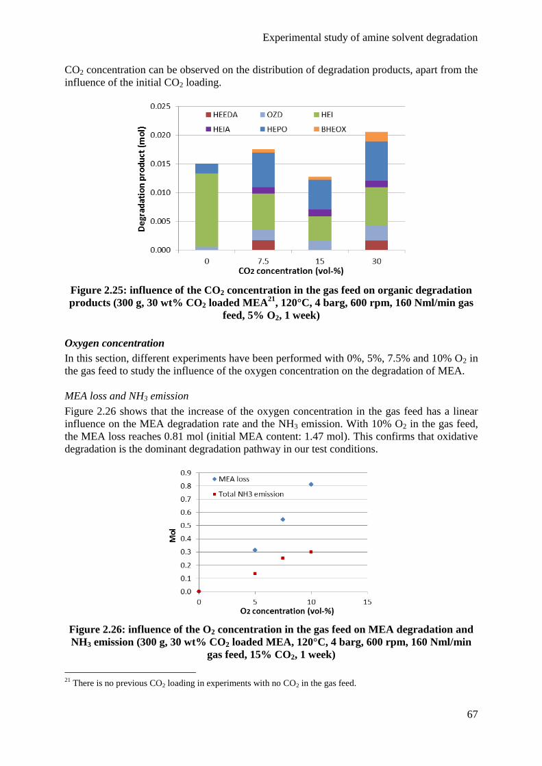
Experimental study of amine solvent degradation

67

CO2 concentration can be observed on the distribution of degradation products, apart from the

influence of the initial CO2 loading.

Figure 2.25: influence of the CO2 concentration in the gas feed on organic degradation

products (300 g, 30 wt% CO2 loaded MEA21

, 120°C, 4 barg, 600 rpm, 160 Nml/min gas

feed, 5% O2, 1 week)

Oxygen concentration

In this section, different experiments have been performed with 0%, 5%, 7.5% and 10% O2 in

the gas feed to study the influence of the oxygen concentration on the degradation of MEA.

MEA loss and NH3 emission

Figure 2.26 shows that the increase of the oxygen concentration in the gas feed has a linear

influence on the MEA degradation rate and the NH3 emission. With 10% O2 in the gas feed,

the MEA loss reaches 0.81 mol (initial MEA content: 1.47 mol). This confirms that oxidative

degradation is the dominant degradation pathway in our test conditions.

Figure 2.26: influence of the O2 concentration in the gas feed on MEA degradation and

NH3 emission (300 g, 30 wt% CO2 loaded MEA, 120°C, 4 barg, 600 rpm, 160 Nml/min

gas feed, 15% CO2, 1 week)

21

There is no previous CO2 loading in experiments with no CO2 in the gas feed.

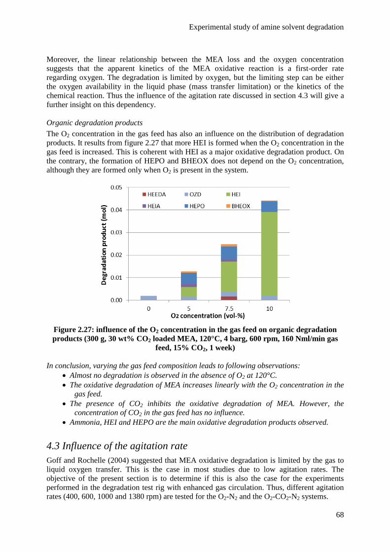
Experimental study of amine solvent degradation

68

Moreover, the linear relationship between the MEA loss and the oxygen concentration

suggests that the apparent kinetics of the MEA oxidative reaction is a first-order rate

regarding oxygen. The degradation is limited by oxygen, but the limiting step can be either

the oxygen availability in the liquid phase (mass transfer limitation) or the kinetics of the

chemical reaction. Thus the influence of the agitation rate discussed in section 4.3 will give a

further insight on this dependency.

Organic degradation products

The O2 concentration in the gas feed has also an influence on the distribution of degradation

products. It results from figure 2.27 that more HEI is formed when the O2 concentration in the

gas feed is increased. This is coherent with HEI as a major oxidative degradation product. On

the contrary, the formation of HEPO and BHEOX does not depend on the O2 concentration,

although they are formed only when O2 is present in the system.

Figure 2.27: influence of the O2 concentration in the gas feed on organic degradation

products (300 g, 30 wt% CO2 loaded MEA, 120°C, 4 barg, 600 rpm, 160 Nml/min gas

feed, 15% CO2, 1 week)

In conclusion, varying the gas feed composition leads to following observations:

Almost no degradation is observed in the absence of O2 at 120°C.

The oxidative degradation of MEA increases linearly with the O2 concentration in the

gas feed.

The presence of CO2 inhibits the oxidative degradation of MEA. However, the

concentration of CO2 in the gas feed has no influence.

Ammonia, HEI and HEPO are the main oxidative degradation products observed.

4.3 Influence of the agitation rate

Goff and Rochelle (2004) suggested that MEA oxidative degradation is limited by the gas to

liquid oxygen transfer. This is the case in most studies due to low agitation rates. The

objective of the present section is to determine if this is also the case for the experiments

performed in the degradation test rig with enhanced gas circulation. Thus, different agitation

rates (400, 600, 1000 and 1380 rpm) are tested for the O2-N2 and the O2-CO2-N2 systems.

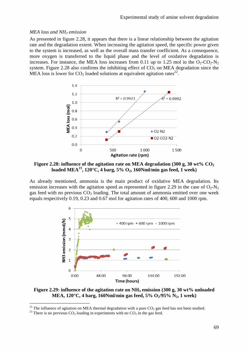
Experimental study of amine solvent degradation

69

MEA loss and NH3 emission

As presented in figure 2.28, it appears that there is a linear relationship between the agitation

rate and the degradation extent. When increasing the agitation speed, the specific power given

to the system is increased, as well as the overall mass transfer coefficient. As a consequence,

more oxygen is transferred to the liquid phase and the level of oxidative degradation is

increases. For instance, the MEA loss increases from 0.11 up to 1.25 mol in the O2-CO2-N2

system. Figure 2.28 also confirms the inhibiting effect of CO2 on MEA degradation since the

MEA loss is lower for CO2 loaded solutions at equivalent agitation rates22

.

Figure 2.28: influence of the agitation rate on MEA degradation (300 g, 30 wt% CO2

loaded MEA23

, 120°C, 4 barg, 5% O2, 160Nml/min gas feed, 1 week)

As already mentioned, ammonia is the main product of oxidative MEA degradation. Its

emission increases with the agitation speed as represented in figure 2.29 in the case of O2-N2

gas feed with no previous CO2 loading. The total amount of ammonia emitted over one week

equals respectively 0.19, 0.23 and 0.67 mol for agitation rates of 400, 600 and 1000 rpm.

Figure 2.29: influence of the agitation rate on NH3 emission (300 g, 30 wt% unloaded

MEA, 120°C, 4 barg, 160Nml/min gas feed, 5% O2/95% N2, 1 week)

22

The influence of agitation on MEA thermal degradation with a pure CO2 gas feed has not been studied. 23

There is no previous CO2 loading in experiments with no CO2 in the gas feed.

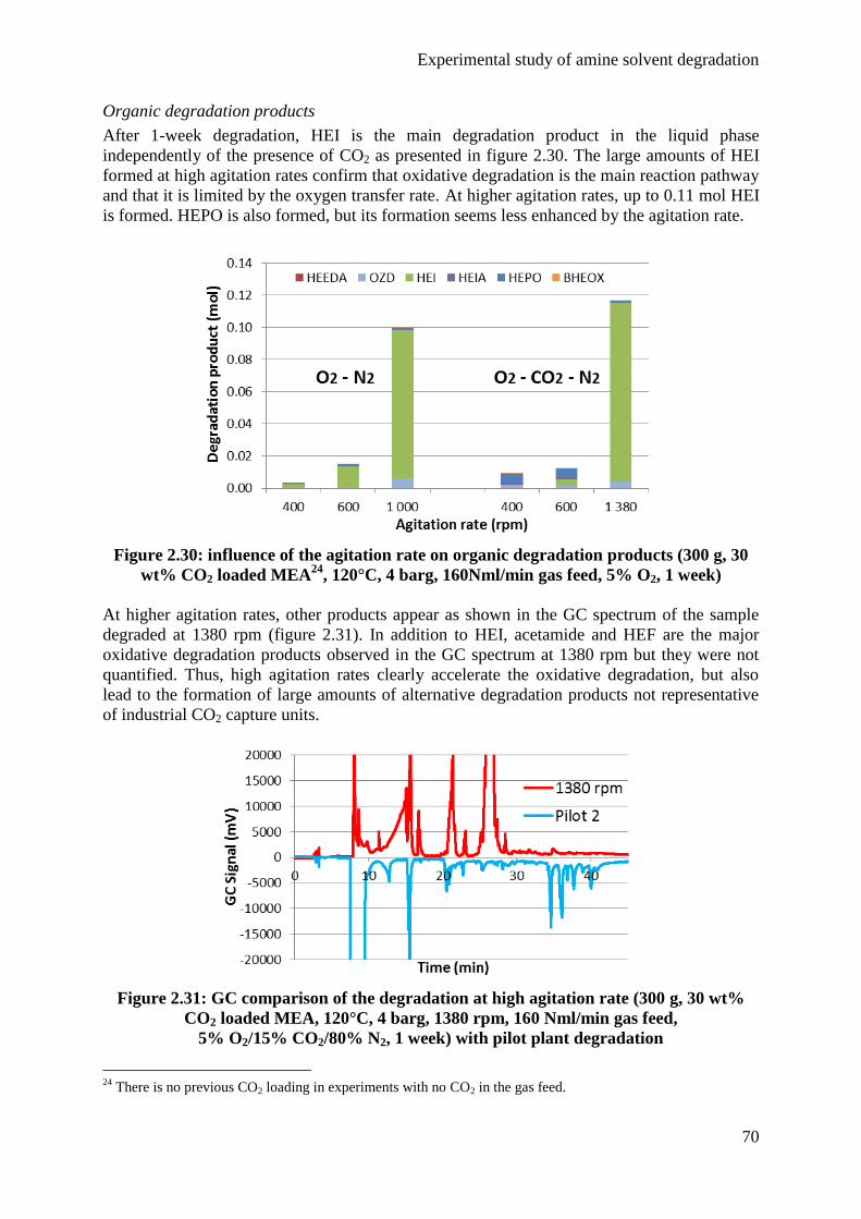
Experimental study of amine solvent degradation

70

Organic degradation products

After 1-week degradation, HEI is the main degradation product in the liquid phase

independently of the presence of CO2 as presented in figure 2.30. The large amounts of HEI

formed at high agitation rates confirm that oxidative degradation is the main reaction pathway

and that it is limited by the oxygen transfer rate. At higher agitation rates, up to 0.11 mol HEI

is formed. HEPO is also formed, but its formation seems less enhanced by the agitation rate.

Figure 2.30: influence of the agitation rate on organic degradation products (300 g, 30

wt% CO2 loaded MEA24

, 120°C, 4 barg, 160Nml/min gas feed, 5% O2, 1 week)

At higher agitation rates, other products appear as shown in the GC spectrum of the sample

degraded at 1380 rpm (figure 2.31). In addition to HEI, acetamide and HEF are the major

oxidative degradation products observed in the GC spectrum at 1380 rpm but they were not

quantified. Thus, high agitation rates clearly accelerate the oxidative degradation, but also

lead to the formation of large amounts of alternative degradation products not representative

of industrial CO2 capture units.

Figure 2.31: GC comparison of the degradation at high agitation rate (300 g, 30 wt%

CO2 loaded MEA, 120°C, 4 barg, 1380 rpm, 160 Nml/min gas feed,

5% O2/15% CO2/80% N2, 1 week) with pilot plant degradation

24

There is no previous CO2 loading in experiments with no CO2 in the gas feed.

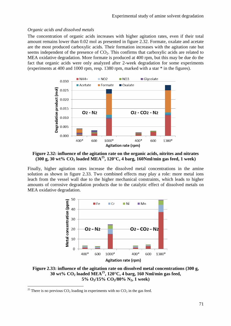
Experimental study of amine solvent degradation

71

Organic acids and dissolved metals

The concentration of organic acids increases with higher agitation rates, even if their total

amount remains lower than 0.02 mol as presented in figure 2.32. Formate, oxalate and acetate

are the most produced carboxylic acids. Their formation increases with the agitation rate but

seems independent of the presence of CO2. This confirms that carboxylic acids are related to

MEA oxidative degradation. More formate is produced at 400 rpm, but this may be due do the

fact that organic acids were only analyzed after 2-week degradation for some experiments

(experiments at 400 and 1000 rpm, resp. 1380 rpm, marked with a star * in the figures).

Figure 2.32: influence of the agitation rate on the organic acids, nitrites and nitrates

(300 g, 30 wt% CO2 loaded MEA25

, 120°C, 4 barg, 160Nml/min gas feed, 1 week)

Finally, higher agitation rates increase the dissolved metal concentrations in the amine

solution as shown in figure 2.33. Two combined effects may play a role: more metal ions

leach from the vessel wall due to the higher mechanical constraints, which leads to higher

amounts of corrosive degradation products due to the catalytic effect of dissolved metals on

MEA oxidative degradation.

Figure 2.33: influence of the agitation rate on dissolved metal concentrations (300 g,

30 wt% CO2 loaded MEA25

, 120°C, 4 barg, 160 Nml/min gas feed,

5% O2/15% CO2/80% N2, 1 week)

25

There is no previous CO2 loading in experiments with no CO2 in the gas feed.

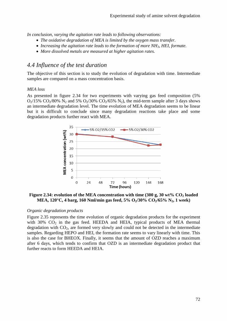
Experimental study of amine solvent degradation

72

In conclusion, varying the agitation rate leads to following observations:

The oxidative degradation of MEA is limited by the oxygen mass transfer.

Increasing the agitation rate leads to the formation of more NH3, HEI, formate.

More dissolved metals are measured at higher agitation rates.

4.4 Influence of the test duration

The objective of this section is to study the evolution of degradation with time. Intermediate

samples are compared on a mass concentration basis.

MEA loss

As presented in figure 2.34 for two experiments with varying gas feed composition (5%

O2/15% CO2/80% N2 and 5% O2/30% CO2/65% N2), the mid-term sample after 3 days shows

an intermediate degradation level. The time evolution of MEA degradation seems to be linear

but it is difficult to conclude since many degradation reactions take place and some

degradation products further react with MEA.

Figure 2.34: evolution of the MEA concentration with time (300 g, 30 wt% CO2 loaded

MEA, 120°C, 4 barg, 160 Nml/min gas feed, 5% O2/30% CO2/65% N2, 1 week)

Organic degradation products

Figure 2.35 represents the time evolution of organic degradation products for the experiment

with 30% CO2 in the gas feed. HEEDA and HEIA, typical products of MEA thermal

degradation with CO2, are formed very slowly and could not be detected in the intermediate

samples. Regarding HEPO and HEI, the formation rate seems to vary linearly with time. This

is also the case for BHEOX. Finally, it seems that the amount of OZD reaches a maximum

after 6 days, which tends to confirm that OZD is an intermediate degradation product that

further reacts to form HEEDA and HEIA.

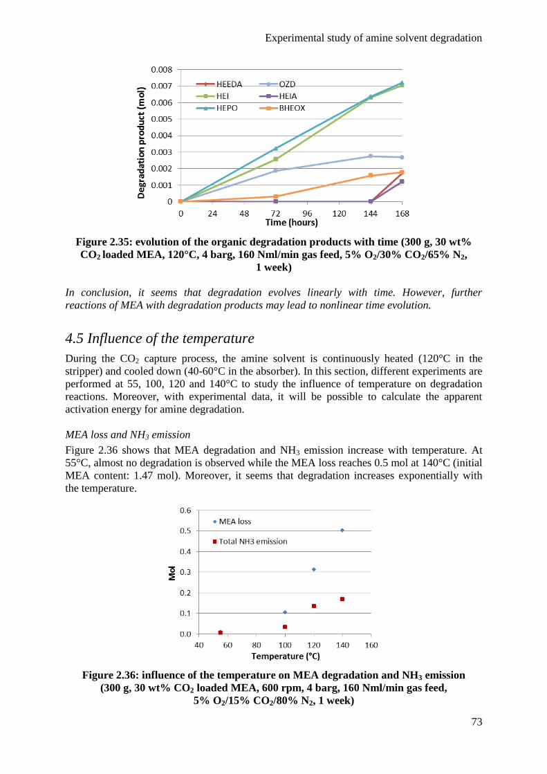
Experimental study of amine solvent degradation

73

Figure 2.35: evolution of the organic degradation products with time (300 g, 30 wt%

CO2 loaded MEA, 120°C, 4 barg, 160 Nml/min gas feed, 5% O2/30% CO2/65% N2,

1 week)

In conclusion, it seems that degradation evolves linearly with time. However, further

reactions of MEA with degradation products may lead to nonlinear time evolution.

4.5 Influence of the temperature

During the CO2 capture process, the amine solvent is continuously heated (120°C in the

stripper) and cooled down (40-60°C in the absorber). In this section, different experiments are

performed at 55, 100, 120 and 140°C to study the influence of temperature on degradation

reactions. Moreover, with experimental data, it will be possible to calculate the apparent

activation energy for amine degradation.

MEA loss and NH3 emission

Figure 2.36 shows that MEA degradation and NH3 emission increase with temperature. At

55°C, almost no degradation is observed while the MEA loss reaches 0.5 mol at 140°C (initial

MEA content: 1.47 mol). Moreover, it seems that degradation increases exponentially with

the temperature.

Figure 2.36: influence of the temperature on MEA degradation and NH3 emission

(300 g, 30 wt% CO2 loaded MEA, 600 rpm, 4 barg, 160 Nml/min gas feed,

5% O2/15% CO2/80% N2, 1 week)

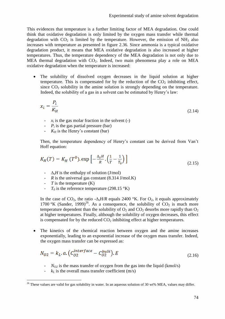
Experimental study of amine solvent degradation

74

This evidences that temperature is a further limiting factor of MEA degradation. One could

think that oxidative degradation is only limited by the oxygen mass transfer while thermal

degradation with CO2 is limited by the temperature. However, the emission of NH3 also

increases with temperature as presented in figure 2.36. Since ammonia is a typical oxidative

degradation product, it means that MEA oxidative degradation is also increased at higher

temperatures. Thus, the temperature dependency of the MEA degradation is not only due to

MEA thermal degradation with CO2. Indeed, two main phenomena play a role on MEA

oxidative degradation when the temperature is increased:

The solubility of dissolved oxygen decreases in the liquid solution at higher

temperature. This is compensated for by the reduction of the CO2 inhibiting effect,

since CO2 solubility in the amine solution is strongly depending on the temperature.

Indeed, the solubility of a gas in a solvent can be estimated by Henry’s law:

(2.14)

- xi is the gas molar fraction in the solvent (-)

- Pi is the gas partial pressure (bar)

- KH is the Henry’s constant (bar)

Then, the temperature dependency of Henry’s constant can be derived from Van’t

Hoff equation:

(2.15)

- ∆sH is the enthalpy of solution (J/mol)

- R is the universal gas constant (8.314 J/mol.K)

- T is the temperature (K)

- T0 is the reference temperature (298.15 °K)

In the case of CO2, the ratio -∆sH/R equals 2400 °K. For O2, it equals approximately

1700 °K (Sander, 1999)26

. As a consequence, the solubility of CO2 is much more

temperature dependent than the solubility of O2 and CO2 desorbs more rapidly than O2

at higher temperatures. Finally, although the solubility of oxygen decreases, this effect

is compensated for by the reduced CO2 inhibiting effect at higher temperatures.

The kinetics of the chemical reaction between oxygen and the amine increases

exponentially, leading to an exponential increase of the oxygen mass transfer. Indeed,

the oxygen mass transfer can be expressed as:

(2.16)

- NO2 is the mass transfer of oxygen from the gas into the liquid (kmol/s)

- kL is the overall mass transfer coefficient (m/s)

26

These values are valid for gas solubility in water. In an aqueous solution of 30 wt% MEA, values may differ.

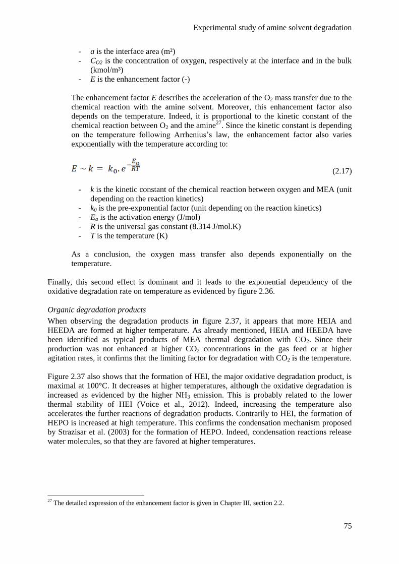
Experimental study of amine solvent degradation

75

- a is the interface area (m²)

- CO2 is the concentration of oxygen, respectively at the interface and in the bulk

(kmol/m³)

- E is the enhancement factor (-)

The enhancement factor E describes the acceleration of the O2 mass transfer due to the

chemical reaction with the amine solvent. Moreover, this enhancement factor also

depends on the temperature. Indeed, it is proportional to the kinetic constant of the

chemical reaction between O2 and the amine27

. Since the kinetic constant is depending

on the temperature following Arrhenius’s law, the enhancement factor also varies

exponentially with the temperature according to:

(2.17)

- k is the kinetic constant of the chemical reaction between oxygen and MEA (unit

depending on the reaction kinetics)

- k0 is the pre-exponential factor (unit depending on the reaction kinetics)

- Ea is the activation energy (J/mol)

- R is the universal gas constant (8.314 J/mol.K)

- T is the temperature (K)

As a conclusion, the oxygen mass transfer also depends exponentially on the

temperature.

Finally, this second effect is dominant and it leads to the exponential dependency of the

oxidative degradation rate on temperature as evidenced by figure 2.36.

Organic degradation products

When observing the degradation products in figure 2.37, it appears that more HEIA and

HEEDA are formed at higher temperature. As already mentioned, HEIA and HEEDA have

been identified as typical products of MEA thermal degradation with CO2. Since their

production was not enhanced at higher CO2 concentrations in the gas feed or at higher

agitation rates, it confirms that the limiting factor for degradation with CO2 is the temperature.

Figure 2.37 also shows that the formation of HEI, the major oxidative degradation product, is

maximal at 100°C. It decreases at higher temperatures, although the oxidative degradation is

increased as evidenced by the higher NH3 emission. This is probably related to the lower

thermal stability of HEI (Voice et al., 2012). Indeed, increasing the temperature also

accelerates the further reactions of degradation products. Contrarily to HEI, the formation of

HEPO is increased at high temperature. This confirms the condensation mechanism proposed

by Strazisar et al. (2003) for the formation of HEPO. Indeed, condensation reactions release

water molecules, so that they are favored at higher temperatures.

27

The detailed expression of the enhancement factor is given in Chapter III, section 2.2.

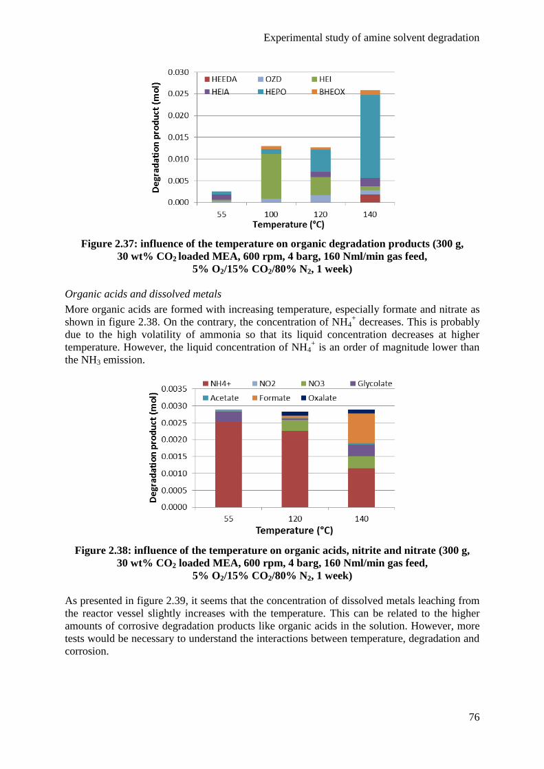
Experimental study of amine solvent degradation

76

Figure 2.37: influence of the temperature on organic degradation products (300 g,

30 wt% CO2 loaded MEA, 600 rpm, 4 barg, 160 Nml/min gas feed,

5% O2/15% CO2/80% N2, 1 week)

Organic acids and dissolved metals

More organic acids are formed with increasing temperature, especially formate and nitrate as

shown in figure 2.38. On the contrary, the concentration of NH4+ decreases. This is probably

due to the high volatility of ammonia so that its liquid concentration decreases at higher

temperature. However, the liquid concentration of NH4+ is an order of magnitude lower than

the NH3 emission.

Figure 2.38: influence of the temperature on organic acids, nitrite and nitrate (300 g,

30 wt% CO2 loaded MEA, 600 rpm, 4 barg, 160 Nml/min gas feed,

5% O2/15% CO2/80% N2, 1 week)

As presented in figure 2.39, it seems that the concentration of dissolved metals leaching from

the reactor vessel slightly increases with the temperature. This can be related to the higher

amounts of corrosive degradation products like organic acids in the solution. However, more

tests would be necessary to understand the interactions between temperature, degradation and

corrosion.

Experimental study of amine solvent degradation

77

Figure 2.39: influence of the temperature on dissolved metal concentrations (300 g,

30 wt% CO2 loaded MEA, 600 rpm, 4 barg, 160 Nml/min gas feed,

5% O2/15% CO2/80% N2, 1 week)

In conclusion, varying the temperature leads to following observations:

The oxidative degradation of MEA seems to increase exponentially with the

temperature. This could be explained by the dependency of the oxygen mass transfer

on temperature.

The formation of NH3, HEPO and formate increases with the temperature, while the

formation of HEI decreases.

4.6 Influence of additives

The objective of this section is to test the influence of dissolved metals on the MEA

degradation rate and to study the potential of inhibitors for reducing the degradation extent.

Dissolved metals

The effect of single metals on MEA degradation has already been described in the literature as

mentioned in section 2.3. Metals enhance the oxidative degradation of MEA due to their

catalytic effect in the formation of free radicals. However, metal leaching from the reactor

vessel has been almost not observed under base case conditions, since the dissolved metal

concentrations at the end of the experiment are lower than 3 ppm for Fe and lower or equal to

1 ppm for Cr, Ni and Mn. Thus, in order to study the influence of dissolved metals on MEA

degradation, a mix of stainless steel metals is added to the solution.

Based on the concentrations of iron, chromium, nickel and manganese measured during a

MEA test campaign on a real CO2 capture plant, corresponding amounts of metal salts have

been added in our experiments. The concentration of dissolved metals in the initial base case

experiment with metal mix has been analyzed by atomic absorption spectroscopy as presented

in table 2.14.

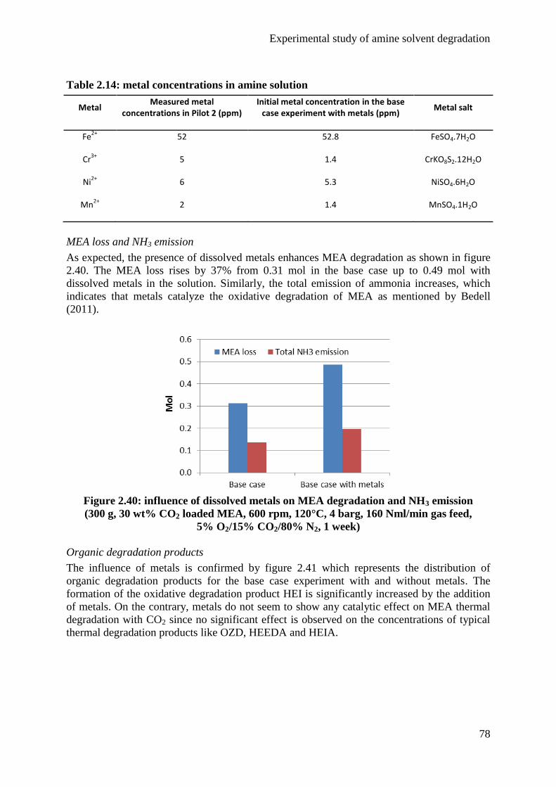
Experimental study of amine solvent degradation

78

Table 2.14: metal concentrations in amine solution

Metal Measured metal

concentrations in Pilot 2 (ppm) Initial metal concentration in the base

case experiment with metals (ppm) Metal salt

Fe2+

52 52.8 FeSO4.7H2O

Cr3+

5 1.4 CrKO8S2.12H2O

Ni2+

6 5.3 NiSO4.6H2O

Mn2+

2 1.4 MnSO4.1H2O

MEA loss and NH3 emission

As expected, the presence of dissolved metals enhances MEA degradation as shown in figure

2.40. The MEA loss rises by 37% from 0.31 mol in the base case up to 0.49 mol with

dissolved metals in the solution. Similarly, the total emission of ammonia increases, which

indicates that metals catalyze the oxidative degradation of MEA as mentioned by Bedell

(2011).

Figure 2.40: influence of dissolved metals on MEA degradation and NH3 emission

(300 g, 30 wt% CO2 loaded MEA, 600 rpm, 120°C, 4 barg, 160 Nml/min gas feed,

5% O2/15% CO2/80% N2, 1 week)

Organic degradation products

The influence of metals is confirmed by figure 2.41 which represents the distribution of

organic degradation products for the base case experiment with and without metals. The

formation of the oxidative degradation product HEI is significantly increased by the addition

of metals. On the contrary, metals do not seem to show any catalytic effect on MEA thermal

degradation with CO2 since no significant effect is observed on the concentrations of typical

thermal degradation products like OZD, HEEDA and HEIA.

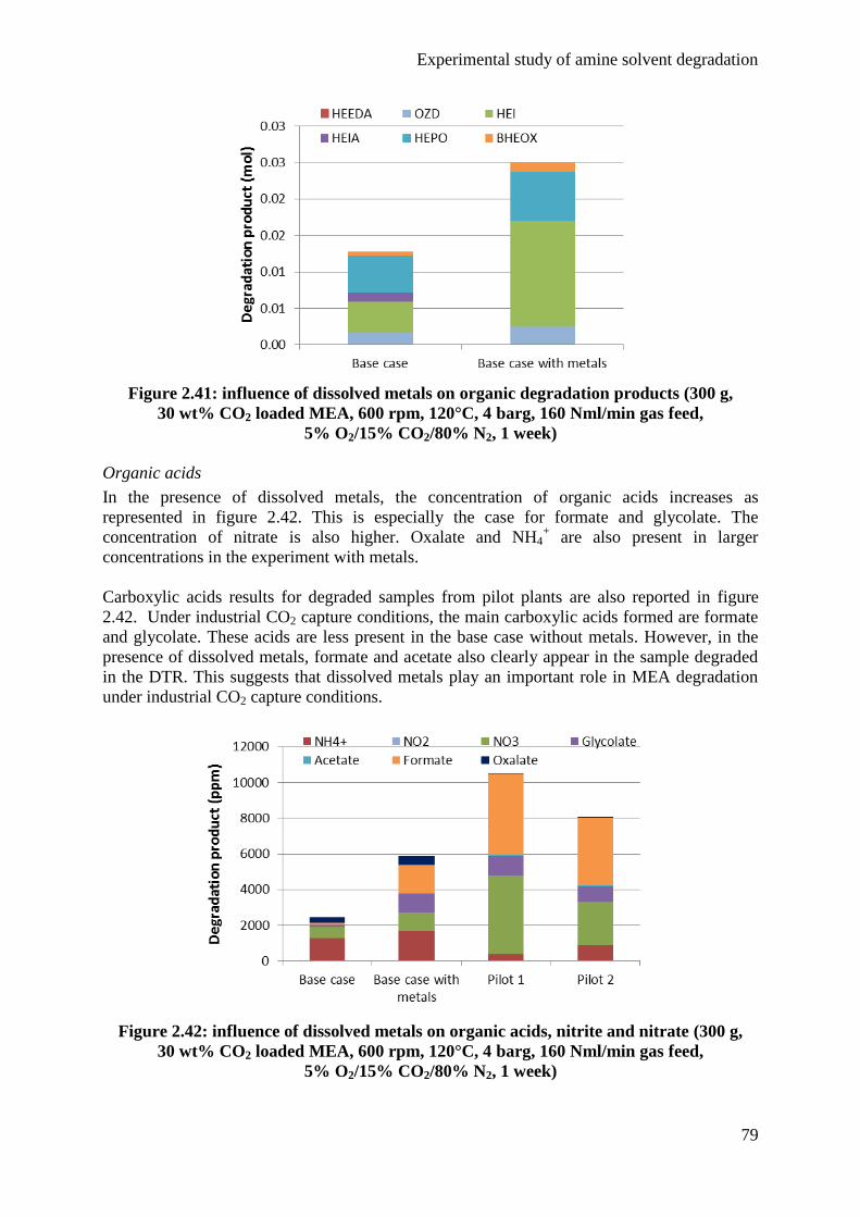
Experimental study of amine solvent degradation

79

Figure 2.41: influence of dissolved metals on organic degradation products (300 g,

30 wt% CO2 loaded MEA, 600 rpm, 120°C, 4 barg, 160 Nml/min gas feed,

5% O2/15% CO2/80% N2, 1 week)

Organic acids

In the presence of dissolved metals, the concentration of organic acids increases as

represented in figure 2.42. This is especially the case for formate and glycolate. The

concentration of nitrate is also higher. Oxalate and NH4+ are also present in larger

concentrations in the experiment with metals.

Carboxylic acids results for degraded samples from pilot plants are also reported in figure

2.42. Under industrial CO2 capture conditions, the main carboxylic acids formed are formate

and glycolate. These acids are less present in the base case without metals. However, in the

presence of dissolved metals, formate and acetate also clearly appear in the sample degraded

in the DTR. This suggests that dissolved metals play an important role in MEA degradation

under industrial CO2 capture conditions.

Figure 2.42: influence of dissolved metals on organic acids, nitrite and nitrate (300 g,

30 wt% CO2 loaded MEA, 600 rpm, 120°C, 4 barg, 160 Nml/min gas feed,

5% O2/15% CO2/80% N2, 1 week)

Experimental study of amine solvent degradation

80

Degradation inhibitors

Based on the literature review summarized in section 2.4, several degradation inhibitors have

been selected and tested in the degradation test rig. So far, these inhibitors have only been

tested in oxidative degradation conditions, i.e. at moderate temperature (~ 55°C-80°C) in the

presence of oxygen. The objective of the present study is to evaluate their influence on MEA

degradation in accelerated degradation conditions.

The following inhibitors have been tested in the degradation test rig:

The first one has been developed at the University of Texas at Austin. Its composition

has not been divulgated, so that it is called “inhibitor A”. One liter of MEA 30 wt%

containing 100 mMol/kg inhibitor A (between 0.5 and 5 wt%) has been received from

Alexander Voice, PhD student at the University of Texas at Austin. Inhibitor A is a

radical scavenger, which means that it reacts with free radicals and stops the

propagation of chain reactions.

The second degradation inhibitor has been patented by the French research institute

IFP Energies Nouvelles. It is called DMTD (dimercaptothiadiazole, C2H2N2S3) and it

also works by reacting with free radicals. 1 wt% of the degradation inhibitor was

added to the amine solution.

The third inhibitor is HEDP (hydroxyethylidene diphosphonic acid, C2H8O7P2 · H2O).

In this case, the inhibition mechanism is different. Indeed, HEDP is a chelating

molecule that forms complexes with metals, so that the catalytic effect of metals is

reduced. 1 wt% of the degradation inhibitor was added to the amine solution.

A combination of 100 mMol/kg inhibitor A with 1 wt% HEDP has also been studied

to observe the combined effect of chelating inhibitors and radical scavengers.

Finally, the thermal stability of different inhibitors including those already mentioned has

been studied in batch reactors (see section 5.3).

In order to get as close as possible to real CO2 capture operations, the metal mix described in

the previous section (Fe2+

, Cr3+

, Ni2+

, Mn2+

) is added to the amine solution with the inhibitor

to be tested. As a consequence, experiments with degradation inhibitors are compared to the

base case with metals described in the previous section. Other operating parameters remain

similar to the initial base case.

MEA loss and NH3 emission

Figure 2.43 presents the MEA loss and the total ammonia emission for each experiment. It

appears that Inhibitor A and DMTD are very efficient. Indeed, the degradation rate is reduced

and very little ammonia is emitted. The decrease of the ammonia emission indicates that

Inhibitor A and DMTD inhibit the oxidative degradation of MEA. On the contrary, HEDP is

not successful at limiting MEA degradation or NH3 emission in the test conditions. Moreover,

the combination of Inhibitor A with HEDP is less efficient than Inhibitor A only.

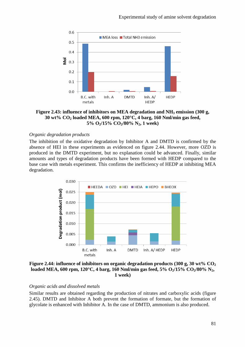
Experimental study of amine solvent degradation

81

Figure 2.43: influence of inhibitors on MEA degradation and NH3 emission (300 g,

30 wt% CO2 loaded MEA, 600 rpm, 120°C, 4 barg, 160 Nml/min gas feed,

5% O2/15% CO2/80% N2, 1 week)

Organic degradation products

The inhibition of the oxidative degradation by Inhibitor A and DMTD is confirmed by the

absence of HEI in these experiments as evidenced on figure 2.44. However, more OZD is

produced in the DMTD experiment, but no explanation could be advanced. Finally, similar

amounts and types of degradation products have been formed with HEDP compared to the

base case with metals experiment. This confirms the inefficiency of HEDP at inhibiting MEA

degradation.

Figure 2.44: influence of inhibitors on organic degradation products (300 g, 30 wt% CO2

loaded MEA, 600 rpm, 120°C, 4 barg, 160 Nml/min gas feed, 5% O2/15% CO2/80% N2,

1 week)

Organic acids and dissolved metals

Similar results are obtained regarding the production of nitrates and carboxylic acids (figure

2.45). DMTD and Inhibitor A both prevent the formation of formate, but the formation of

glycolate is enhanced with Inhibitor A. In the case of DMTD, ammonium is also produced.

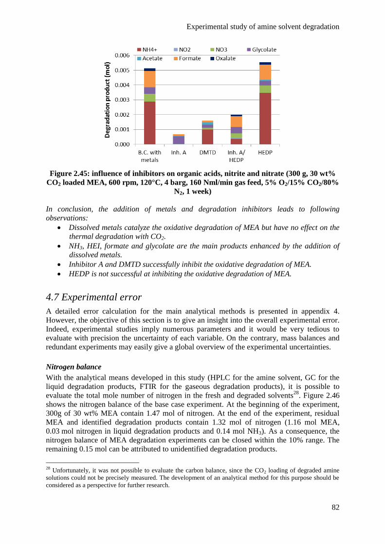
Experimental study of amine solvent degradation

82

Figure 2.45: influence of inhibitors on organic acids, nitrite and nitrate (300 g, 30 wt%

CO2 loaded MEA, 600 rpm, 120°C, 4 barg, 160 Nml/min gas feed, 5% O2/15% CO2/80%

N2, 1 week)

In conclusion, the addition of metals and degradation inhibitors leads to following

observations:

Dissolved metals catalyze the oxidative degradation of MEA but have no effect on the

thermal degradation with CO2.

NH3, HEI, formate and glycolate are the main products enhanced by the addition of

dissolved metals.

Inhibitor A and DMTD successfully inhibit the oxidative degradation of MEA.

HEDP is not successful at inhibiting the oxidative degradation of MEA.

4.7 Experimental error

A detailed error calculation for the main analytical methods is presented in appendix 4.

However, the objective of this section is to give an insight into the overall experimental error.

Indeed, experimental studies imply numerous parameters and it would be very tedious to

evaluate with precision the uncertainty of each variable. On the contrary, mass balances and

redundant experiments may easily give a global overview of the experimental uncertainties.

Nitrogen balance

With the analytical means developed in this study (HPLC for the amine solvent, GC for the

liquid degradation products, FTIR for the gaseous degradation products), it is possible to

evaluate the total mole number of nitrogen in the fresh and degraded solvents28

. Figure 2.46

shows the nitrogen balance of the base case experiment. At the beginning of the experiment,

300g of 30 wt% MEA contain 1.47 mol of nitrogen. At the end of the experiment, residual

MEA and identified degradation products contain 1.32 mol of nitrogen (1.16 mol MEA,

0.03 mol nitrogen in liquid degradation products and 0.14 mol NH3). As a consequence, the

nitrogen balance of MEA degradation experiments can be closed within the 10% range. The

remaining 0.15 mol can be attributed to unidentified degradation products.

28

Unfortunately, it was not possible to evaluate the carbon balance, since the CO2 loading of degraded amine

solutions could not be precisely measured. The development of an analytical method for this purpose should be

considered as a perspective for further research.

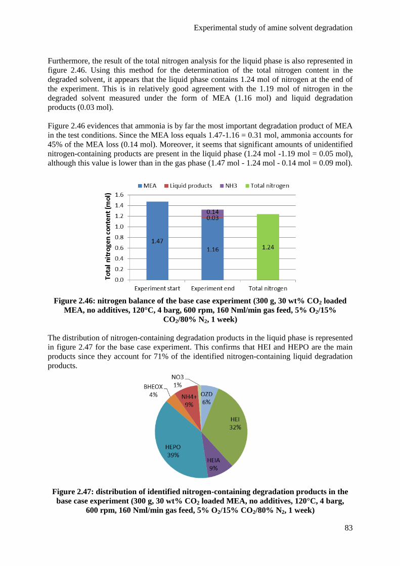
Experimental study of amine solvent degradation

83

Furthermore, the result of the total nitrogen analysis for the liquid phase is also represented in

figure 2.46. Using this method for the determination of the total nitrogen content in the

degraded solvent, it appears that the liquid phase contains 1.24 mol of nitrogen at the end of

the experiment. This is in relatively good agreement with the 1.19 mol of nitrogen in the

degraded solvent measured under the form of MEA (1.16 mol) and liquid degradation

products (0.03 mol).

Figure 2.46 evidences that ammonia is by far the most important degradation product of MEA

in the test conditions. Since the MEA loss equals 1.47-1.16 = 0.31 mol, ammonia accounts for

45% of the MEA loss (0.14 mol). Moreover, it seems that significant amounts of unidentified

nitrogen-containing products are present in the liquid phase (1.24 mol -1.19 mol = 0.05 mol),

although this value is lower than in the gas phase (1.47 mol - 1.24 mol - 0.14 mol = 0.09 mol).

Figure 2.46: nitrogen balance of the base case experiment (300 g, 30 wt% CO2 loaded

MEA, no additives, 120°C, 4 barg, 600 rpm, 160 Nml/min gas feed, 5% O2/15%

CO2/80% N2, 1 week)

The distribution of nitrogen-containing degradation products in the liquid phase is represented

in figure 2.47 for the base case experiment. This confirms that HEI and HEPO are the main

products since they account for 71% of the identified nitrogen-containing liquid degradation

products.

Figure 2.47: distribution of identified nitrogen-containing degradation products in the

base case experiment (300 g, 30 wt% CO2 loaded MEA, no additives, 120°C, 4 barg,

600 rpm, 160 Nml/min gas feed, 5% O2/15% CO2/80% N2, 1 week)

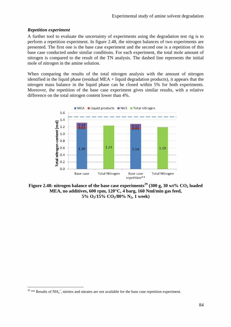
Experimental study of amine solvent degradation

84

Repetition experiment

A further tool to evaluate the uncertainty of experiments using the degradation test rig is to

perform a repetition experiment. In figure 2.48, the nitrogen balances of two experiments are

presented. The first one is the base case experiment and the second one is a repetition of this

base case conducted under similar conditions. For each experiment, the total mole amount of

nitrogen is compared to the result of the TN analysis. The dashed line represents the initial

mole of nitrogen in the amine solution.

When comparing the results of the total nitrogen analysis with the amount of nitrogen

identified in the liquid phase (residual MEA + liquid degradation products), it appears that the

nitrogen mass balance in the liquid phase can be closed within 5% for both experiments.

Moreover, the repetition of the base case experiment gives similar results, with a relative

difference on the total nitrogen content lower than 4%.

Figure 2.48: nitrogen balance of the base case experiments29

(300 g, 30 wt% CO2 loaded

MEA, no additives, 600 rpm, 120°C, 4 barg, 160 Nml/min gas feed,

5% O2/15% CO2/80% N2, 1 week)

29

** Results of NH4+, nitrites and nitrates are not available for the base case repetition experiment.

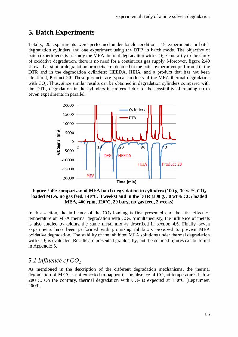
Experimental study of amine solvent degradation

85

5. Batch Experiments

Totally, 20 experiments were performed under batch conditions: 19 experiments in batch

degradation cylinders and one experiment using the DTR in batch mode. The objective of

batch experiments is to study the MEA thermal degradation with CO2. Contrarily to the study

of oxidative degradation, there is no need for a continuous gas supply. Moreover, figure 2.49

shows that similar degradation products are obtained in the batch experiment performed in the

DTR and in the degradation cylinders: HEEDA, HEIA, and a product that has not been

identified, Product 20. These products are typical products of the MEA thermal degradation

with CO2. Thus, since similar results can be obtained in degradation cylinders compared with

the DTR, degradation in the cylinders is preferred due to the possibility of running up to

seven experiments in parallel.

Figure 2.49: comparison of MEA batch degradation in cylinders (100 g, 30 wt% CO2

loaded MEA, no gas feed, 140°C, 3 weeks) and in the DTR (300 g, 30 wt% CO2 loaded

MEA, 400 rpm, 120°C, 20 barg, no gas feed, 2 weeks)

In this section, the influence of the CO2 loading is first presented and then the effect of

temperature on MEA thermal degradation with CO2. Simultaneously, the influence of metals

is also studied by adding the same metal mix as described in section 4.6. Finally, seven

experiments have been performed with promising inhibitors proposed to prevent MEA

oxidative degradation. The stability of the inhibited MEA solutions under thermal degradation

with CO2 is evaluated. Results are presented graphically, but the detailed figures can be found

in Appendix 5.

5.1 Influence of CO2

As mentioned in the description of the different degradation mechanisms, the thermal

degradation of MEA is not expected to happen in the absence of CO2 at temperatures below

200°C. On the contrary, thermal degradation with CO2 is expected at 140°C (Lepaumier,

2008).

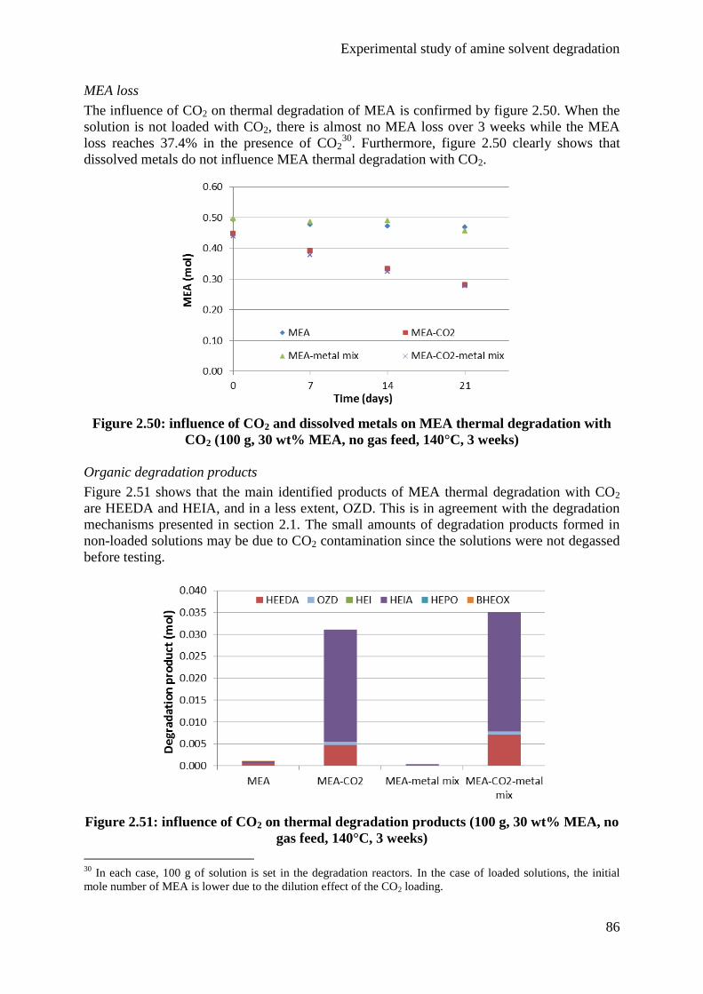
Experimental study of amine solvent degradation

86

MEA loss

The influence of CO2 on thermal degradation of MEA is confirmed by figure 2.50. When the

solution is not loaded with CO2, there is almost no MEA loss over 3 weeks while the MEA

loss reaches 37.4% in the presence of CO230

. Furthermore, figure 2.50 clearly shows that

dissolved metals do not influence MEA thermal degradation with CO2.

Figure 2.50: influence of CO2 and dissolved metals on MEA thermal degradation with

CO2 (100 g, 30 wt% MEA, no gas feed, 140°C, 3 weeks)

Organic degradation products

Figure 2.51 shows that the main identified products of MEA thermal degradation with CO2

are HEEDA and HEIA, and in a less extent, OZD. This is in agreement with the degradation

mechanisms presented in section 2.1. The small amounts of degradation products formed in

non-loaded solutions may be due to CO2 contamination since the solutions were not degassed

before testing.

Figure 2.51: influence of CO2 on thermal degradation products (100 g, 30 wt% MEA, no

gas feed, 140°C, 3 weeks)

30

In each case, 100 g of solution is set in the degradation reactors. In the case of loaded solutions, the initial

mole number of MEA is lower due to the dilution effect of the CO2 loading.

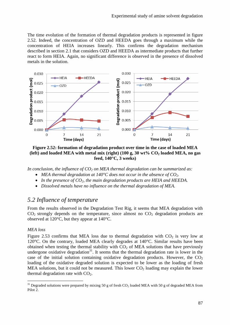
Experimental study of amine solvent degradation

87

The time evolution of the formation of thermal degradation products is represented in figure

2.52. Indeed, the concentration of OZD and HEEDA goes through a maximum while the

concentration of HEIA increases linearly. This confirms the degradation mechanism

described in section 2.1 that considers OZD and HEEDA as intermediate products that further

react to form HEIA. Again, no significant difference is observed in the presence of dissolved

metals in the solution.

Figure 2.52: formation of degradation product over time in the case of loaded MEA

(left) and loaded MEA with metal mix (right) (100 g, 30 wt% CO2 loaded MEA, no gas

feed, 140°C, 3 weeks)

In conclusion, the influence of CO2 on MEA thermal degradation can be summarized as:

MEA thermal degradation at 140°C does not occur in the absence of CO2.

In the presence of CO2, the main degradation products are HEIA and HEEDA.

Dissolved metals have no influence on the thermal degradation of MEA.

5.2 Influence of temperature

From the results observed in the Degradation Test Rig, it seems that MEA degradation with

CO2 strongly depends on the temperature, since almost no CO2 degradation products are

observed at 120°C, but they appear at 140°C.

MEA loss

Figure 2.53 confirms that MEA loss due to thermal degradation with CO2 is very low at

120°C. On the contrary, loaded MEA clearly degrades at 140°C. Similar results have been

obtained when testing the thermal stability with CO2 of MEA solutions that have previously

undergone oxidative degradation31

. It seems that the thermal degradation rate is lower in the

case of the initial solution containing oxidative degradation products. However, the CO2

loading of the oxidative degraded solution is expected to be lower as the loading of fresh

MEA solutions, but it could not be measured. This lower CO2 loading may explain the lower

thermal degradation rate with CO2.

31

Degraded solutions were prepared by mixing 50 g of fresh CO2 loaded MEA with 50 g of degraded MEA from

Pilot 2.

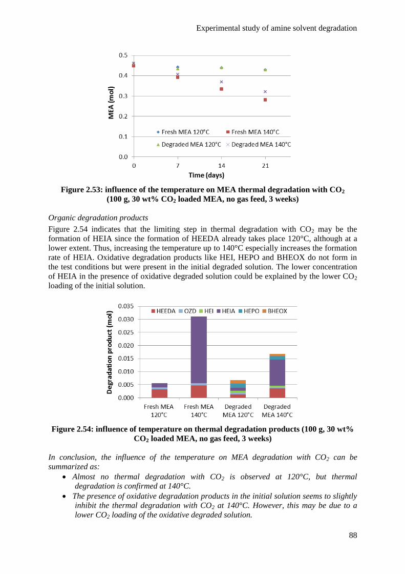
Experimental study of amine solvent degradation

88

Figure 2.53: influence of the temperature on MEA thermal degradation with CO2

(100 g, 30 wt% CO2 loaded MEA, no gas feed, 3 weeks)

Organic degradation products

Figure 2.54 indicates that the limiting step in thermal degradation with CO2 may be the

formation of HEIA since the formation of HEEDA already takes place 120°C, although at a

lower extent. Thus, increasing the temperature up to 140°C especially increases the formation

rate of HEIA. Oxidative degradation products like HEI, HEPO and BHEOX do not form in

the test conditions but were present in the initial degraded solution. The lower concentration

of HEIA in the presence of oxidative degraded solution could be explained by the lower CO2

loading of the initial solution.

Figure 2.54: influence of temperature on thermal degradation products (100 g, 30 wt%

CO2 loaded MEA, no gas feed, 3 weeks)

In conclusion, the influence of the temperature on MEA degradation with CO2 can be

summarized as:

Almost no thermal degradation with CO2 is observed at 120°C, but thermal

degradation is confirmed at 140°C.

The presence of oxidative degradation products in the initial solution seems to slightly

inhibit the thermal degradation with CO2 at 140°C. However, this may be due to a

lower CO2 loading of the oxidative degraded solution.

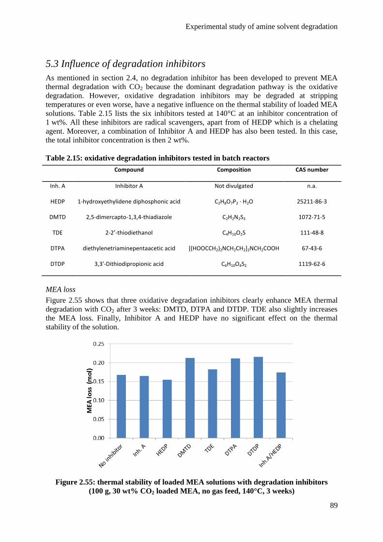
Experimental study of amine solvent degradation

89

5.3 Influence of degradation inhibitors

As mentioned in section 2.4, no degradation inhibitor has been developed to prevent MEA

thermal degradation with CO2 because the dominant degradation pathway is the oxidative

degradation. However, oxidative degradation inhibitors may be degraded at stripping

temperatures or even worse, have a negative influence on the thermal stability of loaded MEA

solutions. Table 2.15 lists the six inhibitors tested at 140°C at an inhibitor concentration of

1 wt%. All these inhibitors are radical scavengers, apart from of HEDP which is a chelating

agent. Moreover, a combination of Inhibitor A and HEDP has also been tested. In this case,

the total inhibitor concentration is then 2 wt%.

Table 2.15: oxidative degradation inhibitors tested in batch reactors

Compound Composition CAS number

Inh. A Inhibitor A Not divulgated n.a.

HEDP 1-hydroxyethylidene diphosphonic acid C2H8O7P2 · H2O 25211-86-3

DMTD 2,5-dimercapto-1,3,4-thiadiazole C2H2N2S3 1072-71-5

TDE 2-2’-thiodiethanol C4H10O2S 111-48-8

DTPA diethylenetriaminepentaacetic acid [(HOOCCH2)2NCH2CH2]2NCH2COOH 67-43-6

DTDP 3,3′-Dithiodipropionic acid C6H10O4S2 1119-62-6

MEA loss

Figure 2.55 shows that three oxidative degradation inhibitors clearly enhance MEA thermal

degradation with CO2 after 3 weeks: DMTD, DTPA and DTDP. TDE also slightly increases

the MEA loss. Finally, Inhibitor A and HEDP have no significant effect on the thermal

stability of the solution.

Figure 2.55: thermal stability of loaded MEA solutions with degradation inhibitors

(100 g, 30 wt% CO2 loaded MEA, no gas feed, 140°C, 3 weeks)

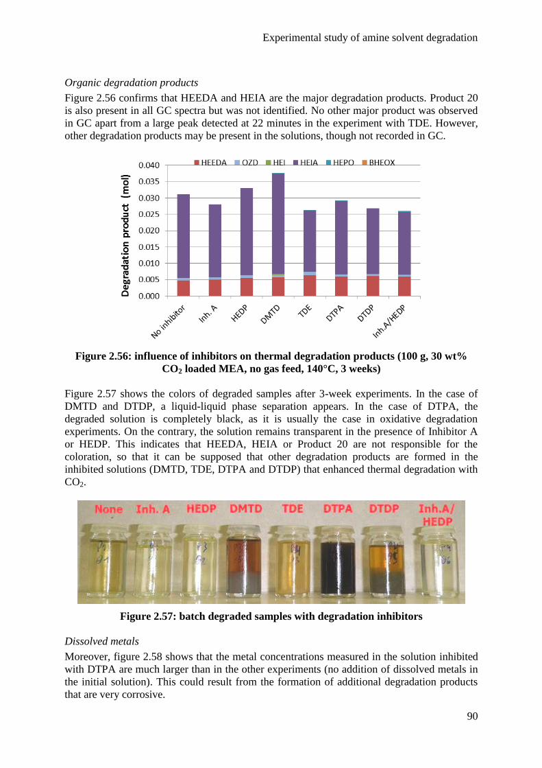
Experimental study of amine solvent degradation

90

Organic degradation products

Figure 2.56 confirms that HEEDA and HEIA are the major degradation products. Product 20

is also present in all GC spectra but was not identified. No other major product was observed

in GC apart from a large peak detected at 22 minutes in the experiment with TDE. However,

other degradation products may be present in the solutions, though not recorded in GC.

Figure 2.56: influence of inhibitors on thermal degradation products (100 g, 30 wt%

CO2 loaded MEA, no gas feed, 140°C, 3 weeks)

Figure 2.57 shows the colors of degraded samples after 3-week experiments. In the case of

DMTD and DTDP, a liquid-liquid phase separation appears. In the case of DTPA, the

degraded solution is completely black, as it is usually the case in oxidative degradation

experiments. On the contrary, the solution remains transparent in the presence of Inhibitor A

or HEDP. This indicates that HEEDA, HEIA or Product 20 are not responsible for the

coloration, so that it can be supposed that other degradation products are formed in the

inhibited solutions (DMTD, TDE, DTPA and DTDP) that enhanced thermal degradation with

CO2.

Figure 2.57: batch degraded samples with degradation inhibitors

Dissolved metals

Moreover, figure 2.58 shows that the metal concentrations measured in the solution inhibited

with DTPA are much larger than in the other experiments (no addition of dissolved metals in

the initial solution). This could result from the formation of additional degradation products

that are very corrosive.

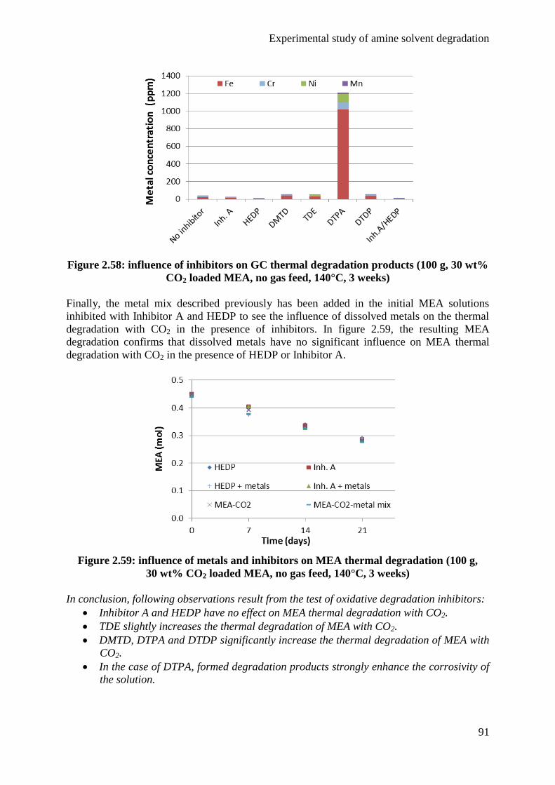
Experimental study of amine solvent degradation

91

Figure 2.58: influence of inhibitors on GC thermal degradation products (100 g, 30 wt%

CO2 loaded MEA, no gas feed, 140°C, 3 weeks)

Finally, the metal mix described previously has been added in the initial MEA solutions

inhibited with Inhibitor A and HEDP to see the influence of dissolved metals on the thermal

degradation with CO2 in the presence of inhibitors. In figure 2.59, the resulting MEA

degradation confirms that dissolved metals have no significant influence on MEA thermal

degradation with CO2 in the presence of HEDP or Inhibitor A.

Figure 2.59: influence of metals and inhibitors on MEA thermal degradation (100 g,

30 wt% CO2 loaded MEA, no gas feed, 140°C, 3 weeks)

In conclusion, following observations result from the test of oxidative degradation inhibitors:

Inhibitor A and HEDP have no effect on MEA thermal degradation with CO2.

TDE slightly increases the thermal degradation of MEA with CO2.

DMTD, DTPA and DTDP significantly increase the thermal degradation of MEA with

CO2.

In the case of DTPA, formed degradation products strongly enhance the corrosivity of

the solution.

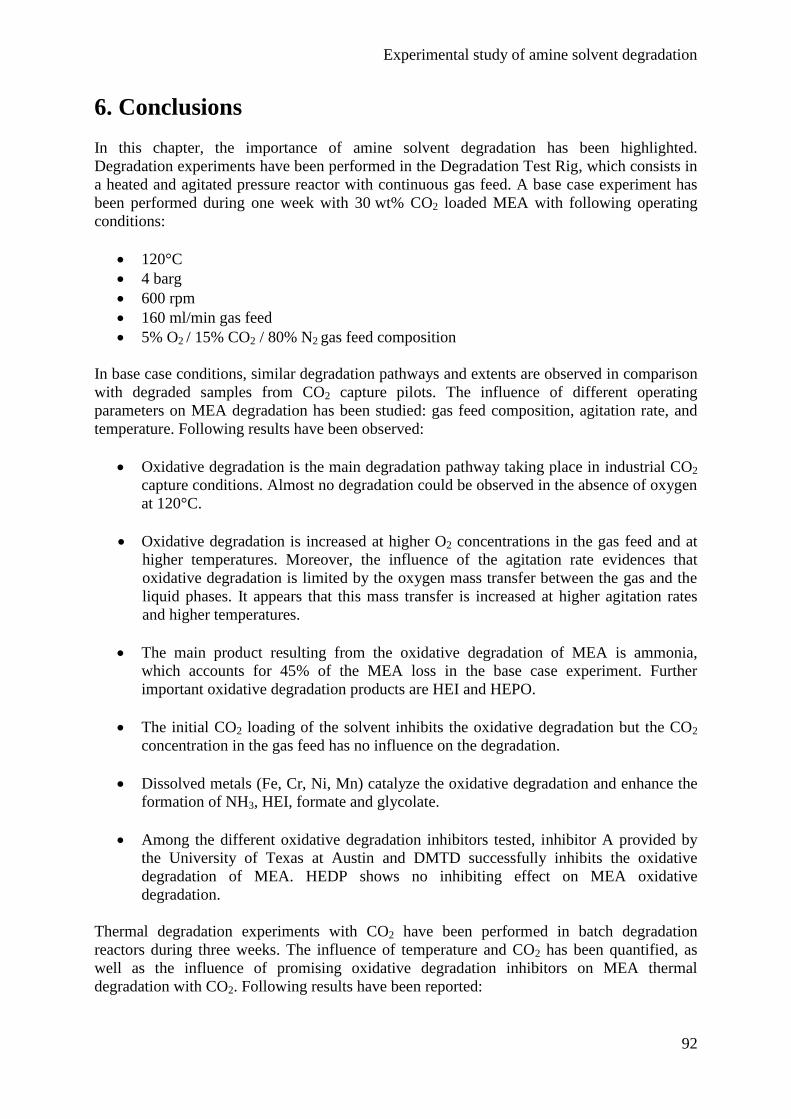
Experimental study of amine solvent degradation

92

6. Conclusions

In this chapter, the importance of amine solvent degradation has been highlighted.

Degradation experiments have been performed in the Degradation Test Rig, which consists in

a heated and agitated pressure reactor with continuous gas feed. A base case experiment has

been performed during one week with 30 wt% CO2 loaded MEA with following operating

conditions:

120°C

4 barg

600 rpm

160 ml/min gas feed

5% O2 / 15% CO2 / 80% N2 gas feed composition

In base case conditions, similar degradation pathways and extents are observed in comparison

with degraded samples from CO2 capture pilots. The influence of different operating

parameters on MEA degradation has been studied: gas feed composition, agitation rate, and

temperature. Following results have been observed:

Oxidative degradation is the main degradation pathway taking place in industrial CO2

capture conditions. Almost no degradation could be observed in the absence of oxygen

at 120°C.

Oxidative degradation is increased at higher O2 concentrations in the gas feed and at

higher temperatures. Moreover, the influence of the agitation rate evidences that

oxidative degradation is limited by the oxygen mass transfer between the gas and the

liquid phases. It appears that this mass transfer is increased at higher agitation rates

and higher temperatures.

The main product resulting from the oxidative degradation of MEA is ammonia,

which accounts for 45% of the MEA loss in the base case experiment. Further

important oxidative degradation products are HEI and HEPO.

The initial CO2 loading of the solvent inhibits the oxidative degradation but the CO2

concentration in the gas feed has no influence on the degradation.

Dissolved metals (Fe, Cr, Ni, Mn) catalyze the oxidative degradation and enhance the

formation of NH3, HEI, formate and glycolate.

Among the different oxidative degradation inhibitors tested, inhibitor A provided by

the University of Texas at Austin and DMTD successfully inhibits the oxidative

degradation of MEA. HEDP shows no inhibiting effect on MEA oxidative

degradation.

Thermal degradation experiments with CO2 have been performed in batch degradation

reactors during three weeks. The influence of temperature and CO2 has been quantified, as

well as the influence of promising oxidative degradation inhibitors on MEA thermal

degradation with CO2. Following results have been reported:

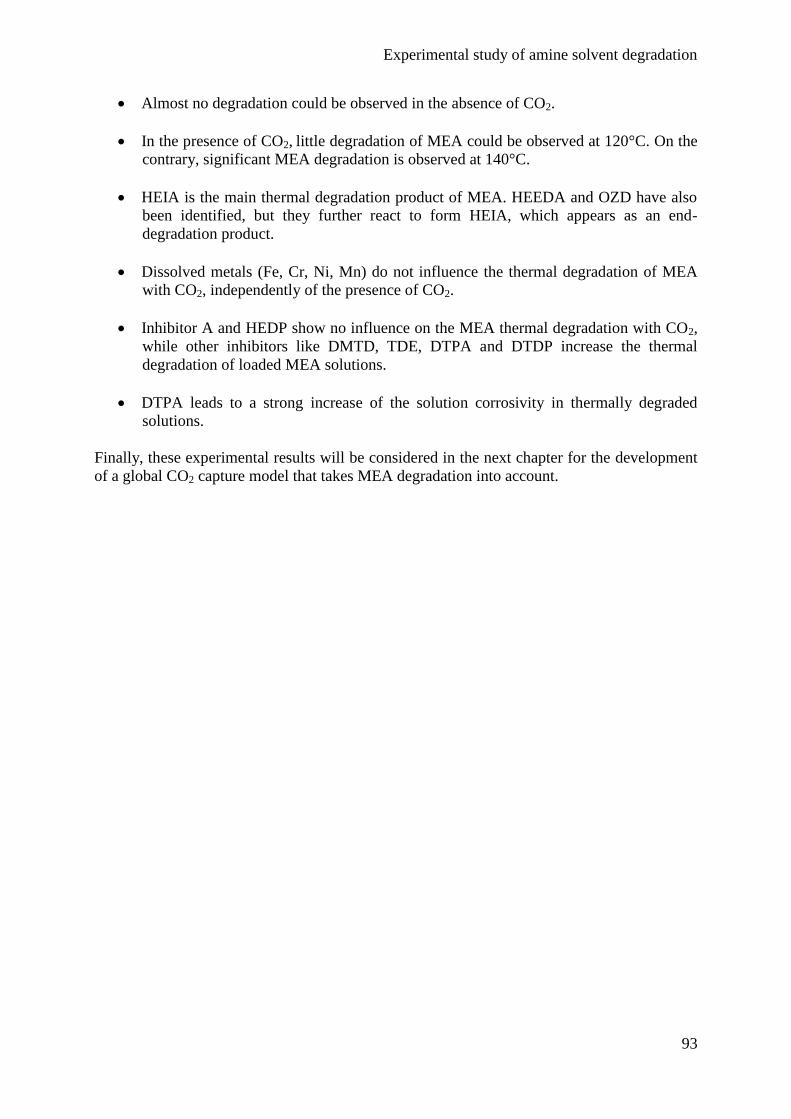
Experimental study of amine solvent degradation

93

Almost no degradation could be observed in the absence of CO2.

In the presence of CO2, little degradation of MEA could be observed at 120°C. On the

contrary, significant MEA degradation is observed at 140°C.

HEIA is the main thermal degradation product of MEA. HEEDA and OZD have also

been identified, but they further react to form HEIA, which appears as an end-

degradation product.

Dissolved metals (Fe, Cr, Ni, Mn) do not influence the thermal degradation of MEA

with CO2, independently of the presence of CO2.

Inhibitor A and HEDP show no influence on the MEA thermal degradation with CO2,

while other inhibitors like DMTD, TDE, DTPA and DTDP increase the thermal

degradation of loaded MEA solutions.

DTPA leads to a strong increase of the solution corrosivity in thermally degraded

solutions.

Finally, these experimental results will be considered in the next chapter for the development

of a global CO2 capture model that takes MEA degradation into account.

Simulation of the CO2 capture process

94

Chapter III

Simulation of the CO2 capture process

“Computers are useless. They can only give you answers.”

Pablo Picasso

Simulation of the CO2 capture process

95

1. Introduction

The main drawback of the CO2 capture process is its large penalty on the power plant

efficiency. Indeed, the energy requirements of CO2 capture units are much larger than the

energy requirement for other environmental control systems installed in current power plants

like desulfurization or denitrification systems. Recently designed supercritical power plants

with high efficiency are less affected by the CO2 capture energy penalty than old low-efficient

plants (Rubin et al., 2012). However, the overall plant efficiency still drops from 40% to 31%

in the case of a new supercritical pulverized coal power plant. This corresponds to an

additional energy input of 29% for a given electricity production.

The energy requirement of a post-combustion CO2 capture plant is composed of three main

parts (ibid.):

~ 60% for thermal solvent regeneration,

~ 30% for CO2 compression,

~ 10% for auxiliary equipment (fans, pumps…).

Moreover, CO2 capture units do not only affect the power plant efficiency. They also impact

the plant water consumption due to the need for cooling and make-up water.

Modeling the capture process is an important part of the technology development. On one

hand, steady-state simulation allows the identification of operating parameters that present the

largest optimization potential without running long and costly experiments. They may be used

to study the influence of process variables on the process efficiency as well as to virtually test

alternative flowsheet configurations that would otherwise induce large costs of equipment

transformation. The objective is to optimize the operating conditions in order to reduce the

process energy penalty. Furthermore, it will be shown in this work that steady-state

simulation can also contribute to the evaluation of the process environmental penalty. Indeed,

when degradation reactions are considered in the simulation, the influence of operating

parameters on the formation of degradation products can be studied. The objective of such

process models including degradation is to find a trade-off between process energy and

environmental penalties.

On the other hand, dynamic simulations are necessary to develop and test control strategies

for operating the capture unit. They may be used to study the process dynamic behavior,

including start-up and shut-down phases as well as transitions between different operating

modes in response to varying steam availability from the power plant.

In this chapter, different pathways are explored for the modeling of the CO2 capture process

with assessment of solvent degradation. First, the main simulation works regarding CO2

capture with amine solvents are briefly presented to give an insight in the state of the art.

Then, four different models are described and their results are discussed:

1. The equilibrium model is a basic model that does not consider any heat and mass

transfer limitations in the absorption and regeneration columns. Chemical kinetics

limitations are also neglected.

Simulation of the CO2 capture process

96

2. The rate-based model considers these limitations. It is compared with the equilibrium

model in order to determine which approach is best suited to describe CO2 capture

processes.

3. The dynamic model is based on the equilibrium model. It is used to study the dynamic

behavior of the process.

4. Finally, the degradation model has been developed in steady-state mode. It is an

improvement of the rate-based model which takes degradation reactions into account.

Moreover, design data have been retrieved from two different pilot plants. The first two

models describe a Mobile Pilot Unit for which the industrial partner Laborelec has been

implied in the design process. The last two models simulate the Esbjerg Pilot Plant, which is a

pilot capture plant developed in the framework of the European projects FP6 CASTOR and

FP7 CESAR.

The impact of operating conditions on the energy penalty is first discussed. Then, an example

of dynamic simulation is presented. Finally, the influence of some key process variables on

the solvent degradation is studied. Some process modifications are also presented and optimal

operating conditions are proposed for the CO2 capture process as a trade-off between

environmental and energy impacts.

Simulation of the CO2 capture process

97

2. State of the art

In this section, the main critical issues when modeling the CO2 capture process are reported

and the solutions proposed in the literature are described. First, the main thermodynamic

methods modeling the properties of amine solutions in the presence of CO2 are presented.

Indeed, electrolyte solutions like amine solvents require a special attention since they show

large deviations from ideality. Then, the phenomena taking place in the absorber and stripper

are considered, since they form the basis of the CO2 capture process. The main modeling

approaches for the hydrodynamics, mass transfer, and chemical reactions related to the

reactive absorption are discussed. Finally, significant steady-state simulation studies of the

CO2 capture process are also presented. Pilot plant models, optimization studies and

simulations of alternative flowsheet configurations are mentioned, as well as some attempts to

include degradation phenomena in the process model. Some dynamic studies of the process

are also mentioned.

2.1 Thermodynamic model

A good thermodynamic model is an essential prerequisite for modeling the CO2 capture

process. Indeed, the macroscopic properties of solvent solutions are determined by variables

like temperature, pressure and component activities in the solution. These variables are

themselves depending on molecular interactions taking place in multi-component solutions. A

suitable description of the molecular interactions is thus essential for estimating the solution

properties, and consequently, for any reliable process modeling.

In the case of solvents for the CO2 capture process, the amine solution contains large

quantities of ionic species called electrolytes. Due to strong inter-molecular interactions,

electrolyte solutions show large deviations from ideality. These non-idealities can be

estimated in two main ways (Austgen, 1989):

Empirical models are using experimentally fitted parameters to correlate equilibrium

relations in electrolyte solutions. They are of practical and simple use since they

require less complex calculations than theoretical models. However, they do not

rigorously calculate the composition of the liquid phase. Furthermore, they usually

show a low predictive potential outside the range of the experimental data used for

parameter fitting. The most used empirical model for amine solutions is the Kent-

Eisenberg model (Kent and Eisenberg, 1976). This model predicts phase equilibrium

data for CO2 and H2S in MEA and DEA solvents by setting all activity coefficients to

unity and determining the value of two equilibrium constants to force a fit with

experimental data. The Kent-Eisenberg model is still used for CO2 capture

applications (e.g. Fouad et al., 2012) and alternative empirical models have been

proposed as well. For instance, the model developed by Gabrielsen et al. (2005)

evaluates vapor-liquid equilibria of three amine systems (MEA, MDEA and DEA)

using four experimentally-regressed parameters. Another model computes apparent

activity coefficients to fit with experimental data for the MEA-H2O-CO2 and the

MDEA-H2O-CO2 systems (Hoff et al., 2004).

Semi-empirical models are based on theoretical assumptions but also imply parameter

adjustment based on experimental data. The main semi-empirical models are the

equations of state and the activity coefficient models. Due to their respective pros and

Simulation of the CO2 capture process

98

cons, these methods are often combined to represent electrolyte solutions. Equations

of state describe the gas phase properties while liquid phase properties are derived

from activity coefficient models. These two types of thermodynamic models are

detailed in the present section.

For comparison purposes, Tobiesen et al. (2008) have modeled and validated a stripping

column for MEA regeneration with two different thermodynamic models. Each model has

been fitted with two different experimental data sets, resulting into four thermodynamic

models. They observed similar model prediction accuracy with the empirical model proposed

by Hoff et al. (2004) and the semi-empirical model of Deshmukh and Mather (1981), as long

as the same experimental data set was used for adjusting thermodynamic model parameters.

However, this was not the case when different data sets were used, highlighting the

importance of reliable experimental data for fitting thermodynamic model parameters.

Activity coefficient models

The composition and subsequently the properties of a mixture depend on two types of

equilibria (Zemaitis et al., 1986)32

:

Phase equilibria are reached when the chemical potential of a component is the same

in all present phases.

Chemical equilibria are reached when the chemical potential of products equals the

chemical potential of reactants.

The variation of the chemical potential of a component with respect to its reference state is

represented by the following:

(3.1)

- µi is the chemical potential of component i (J/mol)

- µi0 is the chemical potential of component i at its reference state (J/mol)

- ai is the activity of component i (-)

- R is the universal gas constant (8.314 J/mol.K)

- T is the temperature (°K)

The reference state is an arbitrarily chosen standard state, usually the pure component at the

system temperature and pressure. This reference state is described as the symmetric reference

state. However, in the case of ions, it is impossible to isolate pure ions, so that the reference

state for ions is the infinite dilution in water. Similarly, the reference state for non-

condensable gases is the infinite dilution in the solvent. This so-called asymmetric reference

state is used in most thermodynamic model of electrolyte solutions. However, a recent study

has proposed the hypothetic state of pure fused salt as the reference state for ions, claiming

for a better consistency in non-aqueous solvents and mixed electrolyte solvents (Song et

Chen, 2009).

32

Solubility equilibria can be considered as a third equilibrium type, but they will not be discussed since no salt

precipitation is observed in the H2O-MEA-CO2 system under usual CO2 capture conditions.

Simulation of the CO2 capture process

99

The chemical activity of a component in a mixture can be described as its normalized active

concentration, or in other terms, as its availability towards a chemical reaction or phase

equilibrium. The relationship between a component’s activity and its mole fraction is

achieved using an activity coefficient γi:

(3.2)

- γi is the activity coefficient of component i (-)

- xi is the mole fraction of component i (-)

Using equations 3.1 and 3.2, the chemical potential of a component in a mixture becomes:

(3.3)

The third term of equation 3.3 is defined as the excess chemical potential µiex

. It reflects the

deviation of the actual chemical potential to ideality. In ideal mixtures, there is no interaction

between the different components so that all activity coefficients tend to unity and the third

term of equation 3.3 equals zero for each component. However, electrolyte solutions present

important deviations from ideality regarding their properties and phase equilibrium

characteristics. In this case, the activity coefficient must be determined for each component.

Besides, the chemical potential of a component can also be defined as the partial Gibbs free

energy at constant temperature, pressure and composition for any component j ≠ i:

(3.4)

- G is the Gibbs free energy (J)

- ni (resp. nj) is the mole number of component i (resp. component j) (mol)

Similarly to the excess chemical potential, the excess Gibbs free energy is defined as the

difference between the actual Gibbs free energy of the mixture and the Gibbs free energy of

an ideal mixture:

(3.5)

From equations 3.3, 3.4 and 3.5, it results that activity coefficients can be derived from the

excess Gibbs free energy:

(3.6)

Many different methods have been proposed to estimate the excess Gibbs free energy or the

activity coefficients of electrolyte systems (Renon, 1996). Most of them are based on the

Debye-Hückel theory that considers electrostatic attraction forces between oppositely charged

ions. The contribution of this ionic attraction must be considered when calculating the Gibbs

Simulation of the CO2 capture process

100

free energy of the system, combined with usual contributions of non-ionic species. Many

different formulations for this electrostatic potential energy have been proposed (e.g.

Guggenheim, 1935; Pitzer, 1973; Deshmukh and Mather, 1981).

Finally, the most used models are perhaps the local contribution models. They are based on a

local contribution model for non-electrolyte solutions, which is then corrected by adding

short-range interaction terms to Gibbs free energy to account for electrostatic interactions.

The basic non-electrolyte local contribution model is the NRTL (nonrandom two-liquid)

model developed by Renon and Prausnitz (1968), which assumes that the local composition

around a molecule is influenced by the interactions of this molecule with its environment. The

NRTL model possesses three main advantages that make it particularly well adapted as a

basis for electrolyte models (Chen, 2006):

It considers local interactions between nearest neighboring species, which is the

central modeling point of view for electrolyte solutions.

It is a model that can be formulated in a simple way from a calculation point of view.

It is widely accepted and used in the industry.

As a consequence, the electrolyte version of this model has been developed and it is currently

one of the most used models for CO2 capture solvents. This electrolyte nonrandom two-liquid

(eNRTL) model is based on two main assumptions (Chen et al., 1982; Chen and Evans,

1986):

Like-ion repulsion: repulsion forces between similarly charged ions (cations or anions)

are extremely large. As a consequence, there is no cation in the local environment of

other cations, and respectively no anion in the local environment of other anions.

Local electro-neutrality: the local ionic charge around a central particle equals zero.

The eNRTL model calculates the activity coefficients of a non-ideal mixture based on the

excess Gibbs free enthalpy of the mixture according to equation 3.7, in which the excess

Gibbs free energy is composed of three terms:

(3.7)

The first term in equation 3.7 is the Pitzer-Debye-Hückel contribution that accounts for long

range ion-ion electrostatic interactions. The reference state for this contribution is the ion

infinite dilution in the mixed solvent. To make it compatible with the reference state of

infinite dilution in water, the Born term is added. This term can be considered as a correction

for the difference between the dielectric constant of water and the mixed solvent for long-

range electrostatic interactions. The third term is the local (or short-range) interaction

contribution and it is the main particularity of the eNRTL model. This term contains binary

parameters that are adjusted on experimental data. More details about these different

contributions to the excess Gibbs energy in the eNRTL model can be found in the literature.

Finally, the eNRTL model has been refined by Bollas et al. (2008). Some simplifying

assumptions of the original model were removed to provide a more rigorous framework for

Simulation of the CO2 capture process

101

the simulation of multi-electrolyte solvents. This refined model has been applied to amine

solvents for CO2 capture by Hessen et al. (2010). However, the increased complexity of this

model makes its implementation unsuitable in its refined form. In conclusion, the initial

eNRTL model has been used in the present work.

Equations of state

Equations of state are very useful to describe thermodynamic properties of both liquid and

vapor phases over a wide range of temperatures and pressures. They require binary

parameters to be fit from experimental vapor-liquid equilibrium data. However, they are not

adapted to describe highly non-ideal mixtures like electrolyte solutions, so that they are only

used for the description of the vapor phase properties in electrolyte systems. Since equations

of state are not particular to electrolyte systems, the theoretical basis of these models are not

detailed in this work but can be easily found in the literature. The most used equations of state

for CO2 capture solvents are the following:

The Redlich-Kwong equation of state (Redlich and Kwong, 1949) is widely used,

especially for addressing hydrocarbon systems.

The Peng-Robinson equation of state (Peng and Robinson, 1976) leads to similar

results compared with the Redlich-Kwong equation in usual pressure and temperature

ranges.

A recent study (van Elk et al., 2009) uses the electrolyte equation of state proposed by

Fürst and Renon (1993) in both liquid and vapor phase. This equation considers an

expression of the Helmholtz free energy instead of the Gibbs free energy. However,

this model is still in development and requires experimental validation.

Finally, the PC-SAFT (Perturbed-Chain Statistical Associating Fluid Theory) equation

of state has been developed by Gross and Sadowski (2001) to describe complex

macromolecular systems. The PC-SAFT equation of state has been successfully

applied to the MEA-H2O-CO2 system by Zhang et al. (2011) to provide accurate vapor

phase fugacity coefficients even at high pressures.

In this work, the Redlich-Kwong equation of state is used for modeling gas phase properties.

2.2 Reactive absorption

CO2 capture in amine solvents is based on the reversible transfer of CO2 from the gas phase

into the liquid phase where it reacts with the amine solvent. The mass transfer and the

chemical reaction of CO2 are taking place in the mass transfer columns which are the central

part of the CO2 capture process. Thus, the fluid hydrodynamics in the columns also plays an

essential role. In other words, three main physical or chemical phenomena take place in the

CO2 capture process:

Hydrodynamics: amine solvent and flue gas flow in counter current through the

column packing. Their intimate contact is maximized by using appropriate column

packing in order to increase the specific interfacial area between gas and liquid and

thus to enhance the CO2 transfer.

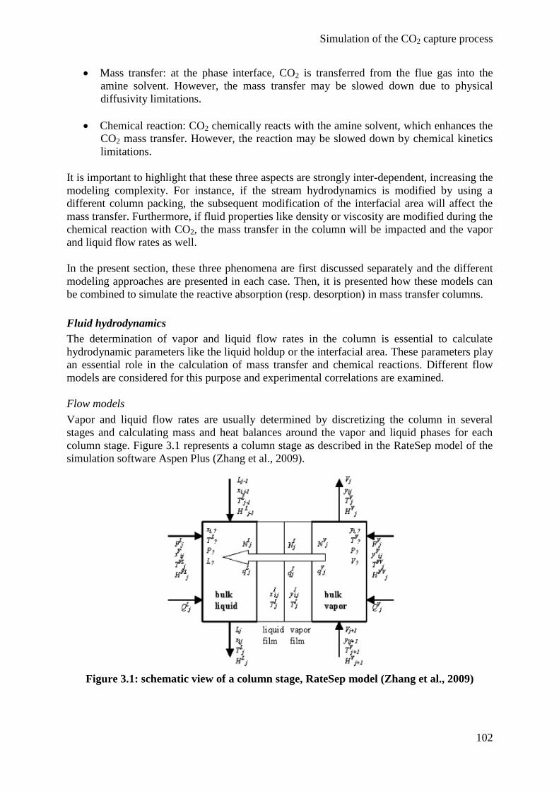
Simulation of the CO2 capture process

102

Mass transfer: at the phase interface, CO2 is transferred from the flue gas into the

amine solvent. However, the mass transfer may be slowed down due to physical

diffusivity limitations.

Chemical reaction: CO2 chemically reacts with the amine solvent, which enhances the

CO2 mass transfer. However, the reaction may be slowed down by chemical kinetics

limitations.

It is important to highlight that these three aspects are strongly inter-dependent, increasing the

modeling complexity. For instance, if the stream hydrodynamics is modified by using a

different column packing, the subsequent modification of the interfacial area will affect the

mass transfer. Furthermore, if fluid properties like density or viscosity are modified during the

chemical reaction with CO2, the mass transfer in the column will be impacted and the vapor

and liquid flow rates as well.

In the present section, these three phenomena are first discussed separately and the different

modeling approaches are presented in each case. Then, it is presented how these models can

be combined to simulate the reactive absorption (resp. desorption) in mass transfer columns.

Fluid hydrodynamics

The determination of vapor and liquid flow rates in the column is essential to calculate

hydrodynamic parameters like the liquid holdup or the interfacial area. These parameters play

an essential role in the calculation of mass transfer and chemical reactions. Different flow

models are considered for this purpose and experimental correlations are examined.

Flow models

Vapor and liquid flow rates are usually determined by discretizing the column in several

stages and calculating mass and heat balances around the vapor and liquid phases for each

column stage. Figure 3.1 represents a column stage as described in the RateSep model of the

simulation software Aspen Plus (Zhang et al., 2009).

Figure 3.1: schematic view of a column stage, RateSep model (Zhang et al., 2009)

Simulation of the CO2 capture process

103

Different flow models are proposed to take bulk properties into account for the determination

of liquid and vapor mass balances, basically considering either a plug flow with low back

mixing or a perfect mixing on each stage:

Mixed flow: the bulk properties for each phase are assumed to be the same as the

outlet conditions of that phase leaving the stage. For instance, the bulk properties of

the liquid on stage j are the same as the bulk properties of the liquid flowing down to

stage j+1.

Countercurrent flow: the bulk properties of each phase are an average between the

inlet and outlet bulk properties.

Vapor plug flow: the liquid bulk properties on a stage are the same as the outlet

conditions for the liquid phase, while the vapor bulk properties are an average between

the inlet and outlet bulk conditions. The outlet pressure is used.

Vapor plug flow with average pressure: bulk properties are determined in the same

way as by the vapor plug flow, only the average value between inlet and outlet

pressures is used.

However, Zhang et al. (2009) show that the flow model has a minor impact on the prediction

of the column performance. They observe no significant difference between the two vapor

plug flow models but report that the mixed flow model describes the column temperature

profile slightly better. As a consequence, the mixed flow model has been selected for the

present study.

An alternative to the discretization of the mass transfer columns in several stages is the use of

Computational Fluid Dynamics (CFD). This method has been recently applied for the detailed

determination of fluid hydrodynamics in CO2 capture columns (Raynal and Royon-Lebeau,

2007; Raynal et al., 2011). This alternative approach allows a rigorous calculation of velocity

fields and a description of the liquid and vapor phase distribution in the column. Moreover, it

can be advantageously used to determine the influence of fluid properties on the stream

hydrodynamics and on the mass transfer parameters. Scale-up of mass transfer columns can

also benefit of that rigorous approach.

Experimental correlations

CFD determination of column hydrodynamics is rather an alternative to measurements since it

requires complex calculations that could hardly be included in a global process simulation.

Thus, since mass transfer calculations require hydrodynamic parameters that cannot be

calculated rigorously, experimental correlations must be used. These correlations are fitted

using experimental data of three types:

Hydrodynamic data (flow velocity, liquid residence time, …)

Fluid properties (viscosity, diffusion coefficient, density, …)

Packing data (characteristic lengths of packing corrugation, specific area, …)

The main hydrodynamic and transfer parameters as well as some reference correlations for

their calculation are listed in table 3.1.

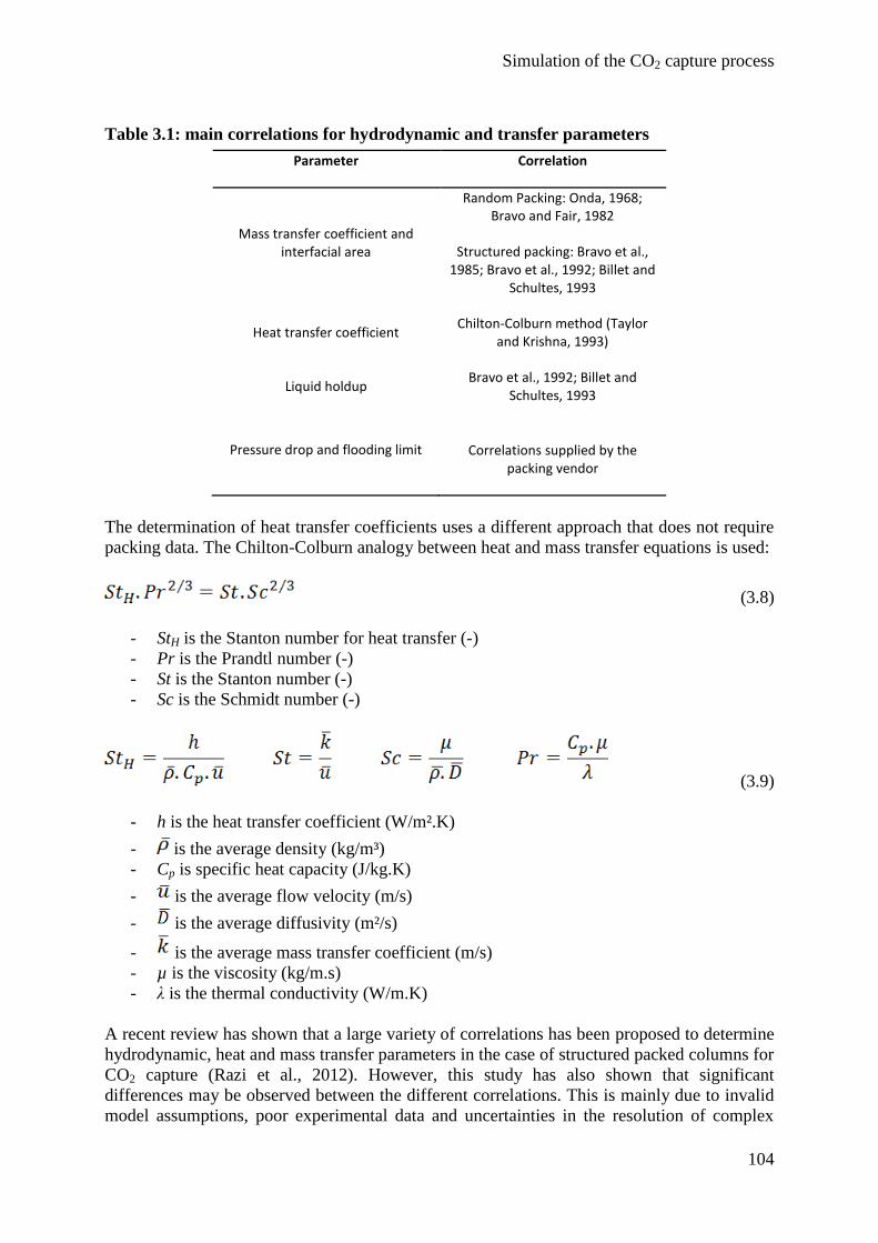
Simulation of the CO2 capture process

104

Table 3.1: main correlations for hydrodynamic and transfer parameters

Parameter Correlation

Mass transfer coefficient and interfacial area

Random Packing: Onda, 1968; Bravo and Fair, 1982

Structured packing: Bravo et al., 1985; Bravo et al., 1992; Billet and

Schultes, 1993

Heat transfer coefficient Chilton-Colburn method (Taylor

and Krishna, 1993)

Liquid holdup Bravo et al., 1992; Billet and

Schultes, 1993

Pressure drop and flooding limit Correlations supplied by the packing vendor

The determination of heat transfer coefficients uses a different approach that does not require

packing data. The Chilton-Colburn analogy between heat and mass transfer equations is used:

(3.8)

- StH is the Stanton number for heat transfer (-)

- Pr is the Prandtl number (-)

- St is the Stanton number (-)

- Sc is the Schmidt number (-)

(3.9)

- h is the heat transfer coefficient (W/m².K)

- is the average density (kg/m³)

- Cp is specific heat capacity (J/kg.K)

- is the average flow velocity (m/s)

- is the average diffusivity (m²/s)

- is the average mass transfer coefficient (m/s)

- µ is the viscosity (kg/m.s)

- λ is the thermal conductivity (W/m.K)

A recent review has shown that a large variety of correlations has been proposed to determine

hydrodynamic, heat and mass transfer parameters in the case of structured packed columns for

CO2 capture (Razi et al., 2012). However, this study has also shown that significant

differences may be observed between the different correlations. This is mainly due to invalid

model assumptions, poor experimental data and uncertainties in the resolution of complex

Simulation of the CO2 capture process

105

equation systems. For instance, Simon et al. (2011) have modeled a CO2 absorption column

using two different approaches for the determination of mass transfer coefficients. Indeed,

they compared the Billet and Schultes correlation (Billet and Schultes, 1999) with

experimentally determined mass transfer coefficients using a wetted-wall bench. They

observed that using laboratory determined mass transfer coefficients improves the model

prediction. The influence of the mass transfer correlation was also confirmed by Tönnies et al.

(2011) using rigorous rate-based calculations for the mass transfer model. Up to 26%

deviation was observed in the CO2 capture rate for the absorber, principally due to large

deviations in the estimation of the interfacial area. Indeed, values ranging from 106 to

471 m²/m³ were calculated, depending on the correlation.

To compensate for correlations uncertainties, simulation packages like Aspen Plus propose

additional factors for adjusting calculated interfacial areas and heat transfer coefficients to

experimental values, so that model validation can be facilitated by fitting these parameters.

The value calculated from the correlation is thus multiplied by this fitting factor provided by

the user to corroborate experimental results.

Finally, the correlations used in the present work are described in section 3.1 and no

experimental fitting parameter has been added.

Mass transfer

There are basically two ways to deal with the modeling of mass transfer phenomena in the

case of reactive absorption:

Equilibrium assumption: this modeling approach considers that mass transfer columns

are composed of successive equilibrium stages. On each stage, a perfect equilibrium is

achieved, so that the liquid phase flowing to the lower stage is in equilibrium with the

gas rising to the upper stage. Mass and heat transfer limitations are neglected.

The rate-based approach: this method implies the rigorous calculation of mass transfer

rates in the column at non-equilibrium conditions. Heat and mass transfer limitations

are taken into account.

Although the first approach is computationally less intensive, it tends to overestimate the

efficiency of the absorption (respectively desorption) process since mass and heat transfer

limitations are neglected. This approach can be corrected using Murphree stage efficiencies,

assuming that only a fraction of the fluid reaches the equilibrium while the remaining fraction

passes unchanged through the stage. This method implying Murphree efficiencies has been

applied to CO2 capture processes by Øi (2012). However, the concept of Murphree stage

efficiency does not rely on any theoretical basis, so that it has only a poor prediction potential.

On the contrary, the rate-based approach is based on theoretical assumptions and the

drawbacks due to more intensive computational calculations are usually compensated for by

an increased model precision. The rate-based modeling is currently the standard state-of-the-

art method for CO2 capture modeling. It requires a good characterization of the fluid

properties, as well as of the column hydrodynamics.

In this section, the main mass transfer models for rate-based calculations are presented.

Different modeling approaches have been proposed to describe the interfacial contact between

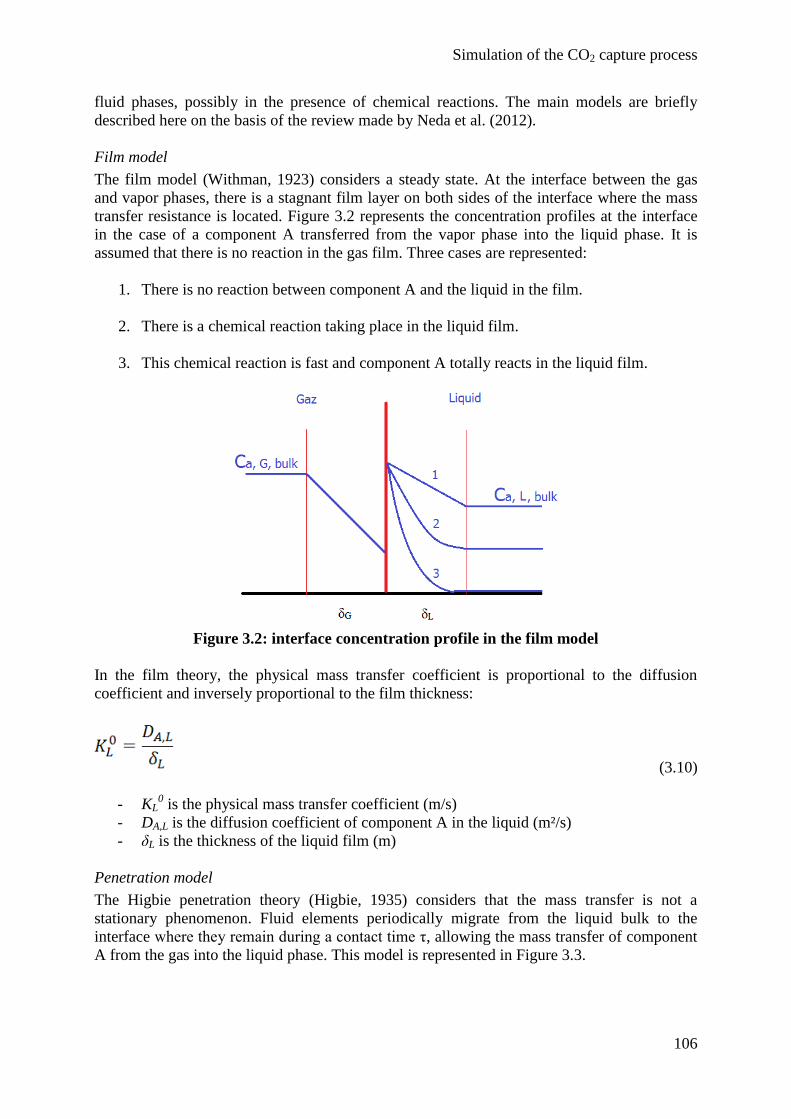
Simulation of the CO2 capture process

106

fluid phases, possibly in the presence of chemical reactions. The main models are briefly

described here on the basis of the review made by Neda et al. (2012).

Film model

The film model (Withman, 1923) considers a steady state. At the interface between the gas

and vapor phases, there is a stagnant film layer on both sides of the interface where the mass

transfer resistance is located. Figure 3.2 represents the concentration profiles at the interface

in the case of a component A transferred from the vapor phase into the liquid phase. It is

assumed that there is no reaction in the gas film. Three cases are represented:

1. There is no reaction between component A and the liquid in the film.

2. There is a chemical reaction taking place in the liquid film.

3. This chemical reaction is fast and component A totally reacts in the liquid film.

Figure 3.2: interface concentration profile in the film model

In the film theory, the physical mass transfer coefficient is proportional to the diffusion

coefficient and inversely proportional to the film thickness:

(3.10)

- KL0 is the physical mass transfer coefficient (m/s)

- DA,L is the diffusion coefficient of component A in the liquid (m²/s)

- δL is the thickness of the liquid film (m)

Penetration model

The Higbie penetration theory (Higbie, 1935) considers that the mass transfer is not a

stationary phenomenon. Fluid elements periodically migrate from the liquid bulk to the

interface where they remain during a contact time τ, allowing the mass transfer of component

A from the gas into the liquid phase. This model is represented in Figure 3.3.

Simulation of the CO2 capture process

107

Figure 3.3: interface concentration profile of the Higbie penetration model

In this model, the physical mass transfer coefficient is proportional to the square root of the

diffusion coefficient:

(3.11)

- τ is the residence time of the liquid at the interface (s)

Surface renewal model

The Danckwerts surface renewal model (Danckwerts, 1951) is based on the same assumption

of unsteady state model as the Higbie penetration model. Furthermore, it considers that

convective movements at the interface (Marangoni effects) lead to a not-constant contact

time. The relationship between the physical mass transfer coefficient and the diffusion

coefficient becomes:

(3.12)

- s is the rate of surface renewal (s-1

)

Finally, it seems that the choice of the mass transfer model is not the most critical issue as

long as the chemical reactions and mass-transfer phenomena are rigorously calculated at the

interface (Tobiesen et al., 2007). In the present work, the equilibrium and the rate-based

approaches have been tested and compared. The mass transfer model used for the rate-based

approach is the film model.

Chemical reactions

Chemical reactions can be modeled in two main ways. The first approach only considers

chemical equilibria that are thermodynamically determined, while the second one takes

chemical kinetics into account.

Equilibrium reactions

In the MEA-CO2-H2O system, the following reactions are taking place in the case of the CO2

capture processes:

Simulation of the CO2 capture process

108

HO-CH2-CH2-NH2 + H3O+ ↔ HO-CH2-CH2-NH3

+ + H2O (3.13)

CO2 + 2 H2O ↔ H3O+ + HCO3

- (3.14)

HCO3- + H2O ↔ H3O

+ + CO3

2- (3.15)

HO-CH2-CH2-NH2 + HCO3- ↔ OH-CH2-CH2-NH-COO

- + H2O (3.16)

2 H2O ↔ H3O+ + OH

- (3.17)

When considering only thermodynamically-determined equilibria, it is assumed that the

reaction rate is so fast that kinetic limitations can be neglected. Thus, the distribution of

reactants and products is calculated based on chemical equilibrium constants defined as:

(3.18)

- Keq is the equilibrium constant (-)

- i is the stoichiometric coefficient of component i in the reaction equation (-)

According to Van’t Hoff’s law, equilibrium constants depend on the temperature according:

(3.19)

- ∆rH is the reaction enthalpy (J/mol)

The equilibrium constants can be calculated in two main ways. First, empirical models can be

used to determine equilibrium constants based on experimental data. Alternatively, when the

thermodynamic fluid properties are precisely calculated, equilibrium constants can be

computed from the reference Gibbs free energies of the components, using the semi-empirical

thermodynamic models described in section 2.1.

Kinetic reactions

Among the reactions listed above, the most critical ones are the reactions describing the

reactive absorption of CO2 (equations 3.14 and 3.16). In the kinetic approach, these reactions

are not considered as instantaneous, so that kinetic limitations must be considered. The

reaction rates are calculated according to:

(3.20)

- r is the reaction rate (kmol/m³.s)

- k0 is the pre-exponential factor [(kmol/m³.s)/((kmol/m³)∑α

i)]

- Ea is the activation energy (J/mol)

- R is the universal gas constant (8.314 J/mol.K)

- T is the temperature (K)

- Ci is the concentration of component i (kmol/m³)

Simulation of the CO2 capture process

109

- N is the number of components (-)

If the stoichiometry of the reaction is known, the only kinetic parameters that must be

experimentally determined are the pre-exponential factor and the activation energy. An

alternative to this equation is to calculate reaction rates based on activities instead of

concentrations. Thus, this leads to:

(3.21)

In this case, the pre-exponential constant is expressed in kmol/m³.s, which is the same unit as

the reaction rate.

Finally, using the phase composition determined either by equilibrium or kinetics reactions,

the fluid properties are evaluated using activity coefficient methods, equations of state, or

empirical models as discussed in the previous section. In the present work, both equilibrium

and kinetics approaches have been used to describe the reaction of CO2 with the amine

solvent.

Reactive absorption models

As already mentioned, fluid hydrodynamics, chemical reactions and mass transfer are

strongly inter-dependent phenomena. In particular, the transfer coefficients determined from a

mass-transfer model may be used to characterize the physical absorption of CO2 in the amine

solvent, but they do not consider the chemical reaction of CO2 with the amine. However,

chemical reactions taking place at the gas-liquid interface strongly enhance the reactive

absorption. Considering mass transfer as independent of chemical equilibria would only lead

to unreliable results. In this section, two main methods to include chemical reactions in the

rate-based mass transfer models are described.

Enhancement factor

The first method consists in defining an enhancement factor E as the ratio of the actual mass

transfer coefficient and the pure physical mass transfer coefficient. The driving force for the

mass transfer of component i is the concentrations difference between the bulk and the

interface. The mass transfer is accelerated by the enhancement factor as following:

(3.22)

- Ni is the mass transfer of component i (kmol/s)

- kL is the overall mass transfer coefficient (m/s)

- a is the interface area (m²)

- Ci is the concentration of component i, respectively at the interface and in the bulk

(kmol/m³)

- E is the enchancement factor (-)

This enhancement factor depends on the reaction kinetics and on the diffusion coefficients of

the components implied in the reaction. Many studies have been performed to evaluate the

enhancement factor in function of the Hatta number, a dimensionless number that compares

the chemical reaction kinetics with the pure physical mass transfer. Considering a first-order

Simulation of the CO2 capture process

110

reaction between absorbed component A and solvent component B taking place in the liquid

phase, the Hatta number can be defined as:

(3.23)

- DA,L is the diffusion coefficient of component A in the liquid phase (m²/s)

- k is the kinetic constant of the chemical reaction between absorbed component A and

solvent component B (L/mol.s)

- CB,L is the concentration of component B in the liquid bulk (mol/L)

- KL0 is the physical mass transfer coefficient (m/s)

Based on the reaction kinetics and on the mass transfer model, different expressions for the

enhancement factor have been proposed. According to Dubois (2013), the mass transfer

model has no significant influence on the numerical value of the enhancement factor.

Faramarzi et al (2010) have compared three expressions of the enhancement factor based on

the film model for the reactive absorption of CO2 in MEA. These expressions are listed in

table 3.2.

Table 3.2: different expressions of the enhancement factor

Enhancement factor Reaction type Reference

Second-order irreversible reaction

Van Krevelen and Hoftijzer, 1948

Second-order irreversible reaction

Astarita et al., 1983

Pseudo-first order reaction Kucka et al., 2003

In the case of a pseudo-first order reaction, the enhancement factor reduces to the Hatta

number33

. Many expressions of the enhancement factor E use the parameter E∞, which is the

enhancement factor for an infinitely fast reaction. In the film theory, it is defined as:

(3.24)

33

The basis assumption for pseudo-first order reaction is that the concentration of solvent B in the film is not

affected by the reaction with absorbing component A. As a consequence, the absorption rate can be written as:

r = k.CA.CB ≈ k’.CA

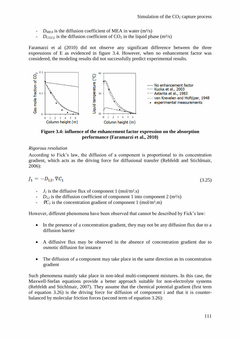
Simulation of the CO2 capture process

111

- DMEA is the diffusion coefficient of MEA in water (m²/s)

- DCO2,L is the diffusion coefficient of CO2 in the liquid phase (m²/s)

Faramarzi et al (2010) did not observe any significant difference between the three

expressions of E as evidenced in figure 3.4. However, when no enhancement factor was

considered, the modeling results did not successfully predict experimental results.

Figure 3.4: influence of the enhancement factor expression on the absorption

performance (Faramarzi et al., 2010)

Rigorous resolution

According to Fick’s law, the diffusion of a component is proportional to its concentration

gradient, which acts as the driving force for diffusional transfer (Rehfeldt and Stichlmair,

2006):

(3.25)

- J1 is the diffusive flux of component 1 (mol/m².s)

- D12 is the diffusion coefficient of component 1 into component 2 (m²/s)

- ∇C1 is the concentration gradient of component 1 (mol/m³.m)

However, different phenomena have been observed that cannot be described by Fick’s law:

In the presence of a concentration gradient, they may not be any diffusion flux due to a

diffusion barrier

A diffusive flux may be observed in the absence of concentration gradient due to

osmotic diffusion for instance

The diffusion of a component may take place in the same direction as its concentration

gradient

Such phenomena mainly take place in non-ideal multi-component mixtures. In this case, the

Maxwell-Stefan equations provide a better approach suitable for non-electrolyte systems

(Rehfeldt and Stichlmair, 2007). They assume that the chemical potential gradient (first term

of equation 3.26) is the driving force for diffusion of component i and that it is counter-

balanced by molecular friction forces (second term of equation 3.26):

Simulation of the CO2 capture process

112

(3.26)

- xi is the mole fraction of component i (-)

- ∇(T,P)µi is the chemical potential gradient of component i at constant temperature and

pressure (J/mol)

- R is the universal gas constant (8.314 J/mol.K)

- T is the temperature (K)

- n is the number of components in the mixture (-)

- Dij is the Maxwell-Stefan diffusivity coefficient (m²/s)

- vi – vj is the velocity difference between components i and j (m/s)

In the case of ideal chemical systems, the Maxwell-Stefan equations reduce to the Fick’s law.

An exact solution of Maxwell-Stefan equations has been proposed by Krishna and Standart

(1976) in the case of a film model.

However, in electrolyte solutions, electric forces play the role of an additional diffusion

driving force, inducing an additional term in the Maxwell-Stefan equations (Ahmadi, 2011).

(3.27)

- zi is the ionic charge of component i (-)

- F is the Faraday constant (96 485 C/mol)

- Φe is the electric potential (V = J/C)

Thus the second method to combine mass transfer and chemical reactions is to perform

rigorous calculations of the Maxwell-Stefan equations including detailed chemistry

calculations. Once again, different mass transfer models can be used like the film model or

the penetration model. The mass transfer rate is not estimated using an enhancement factor

anymore, but is computed from partial mass balances and chemical models calculations. This

method is computationally more intensive but should yield more precise results.

In a recent paper, Meldon and Morales-Cabrera (2011) have compared the numerical

resolution of the Maxwell-Stefan equations with the results of the enhancement factor method

based on the film theory with a pseudo-first order reaction kinetics. They observed excellent

agreement between both methods. Similarly, Tobiesen et al. (2007) have developed a rigorous

absorber model based on the penetration theory. They calculated the resulting enhancement

factor and compared it with three enhancement factor expressions based on the film theory.

All expressions modeled the experimental results quite well, as long as the CO2 loading of the

MEA solvent was low. However, at higher loadings, the enhancement factors based on the

film theory were overestimated and the model prediction was unreliable. Only the rigorous

resolution of the penetration mass transfer model gave acceptable results. Finally, the

simulation tool Aspen Plus that has been used in the present work does not consider

enhancement factors but directly solves the extended Maxwell-Stefan equation.

Simulation of the CO2 capture process

113

2.3 Main modeling studies about CO2 capture with MEA

Many simulation works have been reported in the scientific literature, especially during the

last decade. Most of the published models simulate stationary operating modes. Steady-state

models do not consider the time dependency of process variables, so that calculations are

considerably simplified. Steady-state models may pursue three different objectives, which are

presented in this section. First, they can be used to simulate and accompany the experimental

campaigns of a pilot plant that has been erected. Second, they may be used to study the

influence of process variables and to find the optimal operating conditions. And third, they

may be used to simulate alternative process configurations that may be more difficult to test

experimentally due to cost issues.

Then, some dynamic models of the CO2 capture process are also presented. They take the

time dependency of process variables into account and study the process temporal evolution.

They provide a useful help for transient regime description and may contribute to develop

efficient process control strategies.

Finally, some studies are also presented that consider solvent degradation reactions in the

steady-state process. Both oxidative and thermal degradation of MEA with CO2 are discussed.

Process modeling tools

Different simulation software packages have been used for modeling the CO2 capture process.

Following the discussion presented in section 2.1, the different modeling tools can propose a

variety of thermodynamic models and properties data banks. Finally, they may offer

equilibrium vs. rigorous rate-based calculations of the transfer phenomena, and different

approaches to include (or not) chemical reactions in the mass transfer model may be

proposed. Figure 3.5 graphically summarizes the main modeling features in terms of mass

transfer and reaction precision according to the review published by Kenig et al. (2001).

Some software packages propose graphical interfaces in which the user can build the process

flowsheet by assembling equation blocks. In other software packages, the process equations

must be entered by the user. Some modeling tools have been developed as in-house tools

especially for CO2 capture applications, while other packages are commercially available and

can model a large range of processes. Table 3.3 lists some of the main simulation packages

used for modeling the CO2 capture process (Luo et al., 2009; Øi, 2012). In the present work,

the simulation tool Aspen Plus has been used.

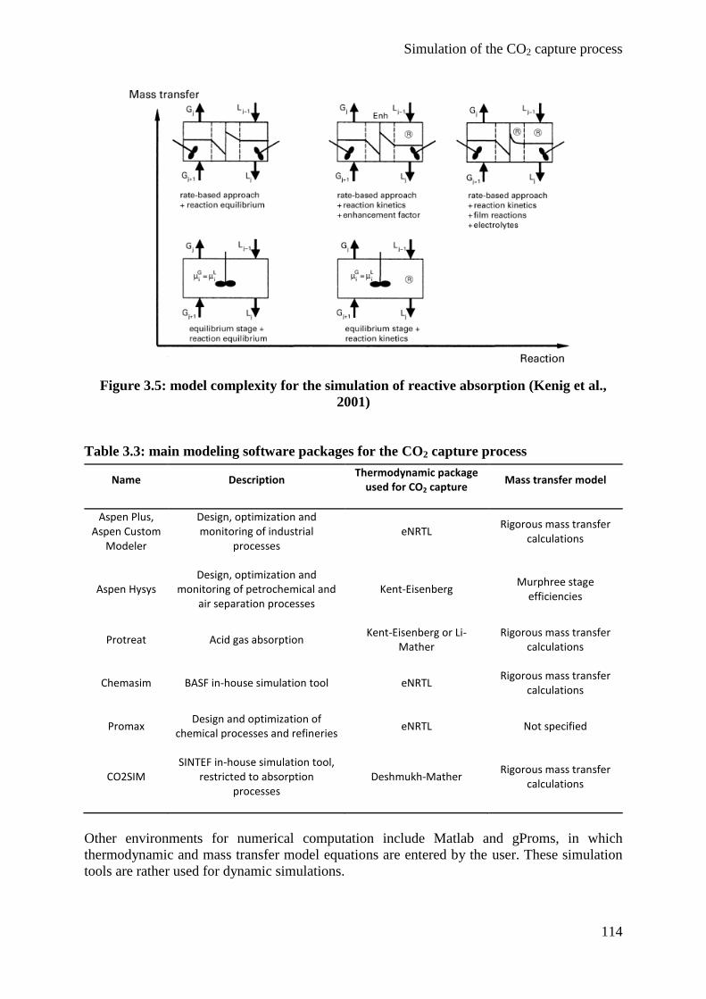
Simulation of the CO2 capture process

114

Figure 3.5: model complexity for the simulation of reactive absorption (Kenig et al.,

2001)

Table 3.3: main modeling software packages for the CO2 capture process

Name Description Thermodynamic package

used for CO2 capture Mass transfer model

Aspen Plus, Aspen Custom

Modeler

Design, optimization and monitoring of industrial

processes eNRTL

Rigorous mass transfer calculations

Aspen Hysys Design, optimization and

monitoring of petrochemical and air separation processes

Kent-Eisenberg Murphree stage

efficiencies

Protreat Acid gas absorption Kent-Eisenberg or Li-

Mather Rigorous mass transfer

calculations

Chemasim BASF in-house simulation tool eNRTL Rigorous mass transfer

calculations

Promax Design and optimization of

chemical processes and refineries eNRTL Not specified

CO2SIM SINTEF in-house simulation tool,

restricted to absorption processes

Deshmukh-Mather Rigorous mass transfer

calculations

Other environments for numerical computation include Matlab and gProms, in which

thermodynamic and mass transfer model equations are entered by the user. These simulation

tools are rather used for dynamic simulations.

Simulation of the CO2 capture process

115

Pilot plant models

Six main pilot units have been described in modeling studies. These units are all reported in

section 3.2 of Chapter I. The modeling studies do not assess the largest pilot units, but rather

small experimental capture units developed for research purposes and for which results are

not confidential. These five pilot units are listed below. All operate with 30 wt% MEA except

if specified elsewise.

The SRP pilot plant at the University of Texas at Austin has been built in 2002 and

modeled in 2009 by Zhang et al. (2009) for 30 wt% MEA. The model has been

developed in Aspen Plus using the eNRTL thermodynamic package and rate-based

mass transfer calculations. The model was also developed using the equilibrium stage

assumption for comparison purpose, and the superiority of the rigorous rate-based

calculation has been evidenced. The influence of rate-based parameters has been

studied and the predictive potential of the model has been highlighted. Plaza et al.

(2009, 2010) have successfully extended this model to 35 wt% MEA and confirmed

the excellent fitting of the model with experimental data.

The Esbjerg pilot plant is the largest pilot unit for which modeling studies have been

published. It started operating in 2006 and simulation results were successfully

compared to experimental results by Dugas et al. (2009) using the rate-based model of

Aspen Plus. Absorber temperature profiles appeared to be slightly over-predicted by

the simulation, while CO2 concentration profiles perfectly fit experimental absorber

data. In his PhD thesis, Abu-Zahra (2009) compared the experimental results to

simulation results obtained with both rate-based and equilibrium stage models. The

superiority of rate-based simulations was confirmed, especially for describing column

temperature profiles.

From 2007, a new simulation package called CO2SIM has been developed at the

Sintef research institute in Norway for modeling post-combustion CO2 capture units.

Tobiesen et al. (2007, 2008) have separately validated the absorber and stripping

columns based on experimental results with an average absolute deviation lower than

10% in all cases. In 2011, a larger pilot plant for CO2 capture, the Tiller pilot, started

operating at the Sintef facility in Trondheim. This new pilot unit was successfully

modeled and validated for flue gas from natural gas combustion by Mejdell et al.

(2011). The Tiller validated model was also used to model and optimize a mobile test

unit developed by Aker Clean Carbon, but no additional model validation has been

performed on the mobile test unit (Tobiesen and Schumann-Olsen, 2011).

The pilot plant at the Technical University of Kaiserslautern has first been modeled by

Notz during his PhD thesis (Notz, 2009) with the simulation tool CHEMASIM. Using

the eNRTL thermodynamic package and a rigorous mass-transfer model, the standard

deviation between experimental and simulation results in the column profiles was kept

under 10% except at high liquid flow rates. In this case, the higher deviation was

explained by a limited validity range for the selected mass transfer correlation.

Tönnies et al. (2011) and Kale et al. (2011) have also modeled this pilot unit using

respectively the Aspen Plus and Aspen Custom Modeler simulation tools. In both

cases, the eNRTL thermodynamic package was used and a rigorous mass transfer

model was applied.

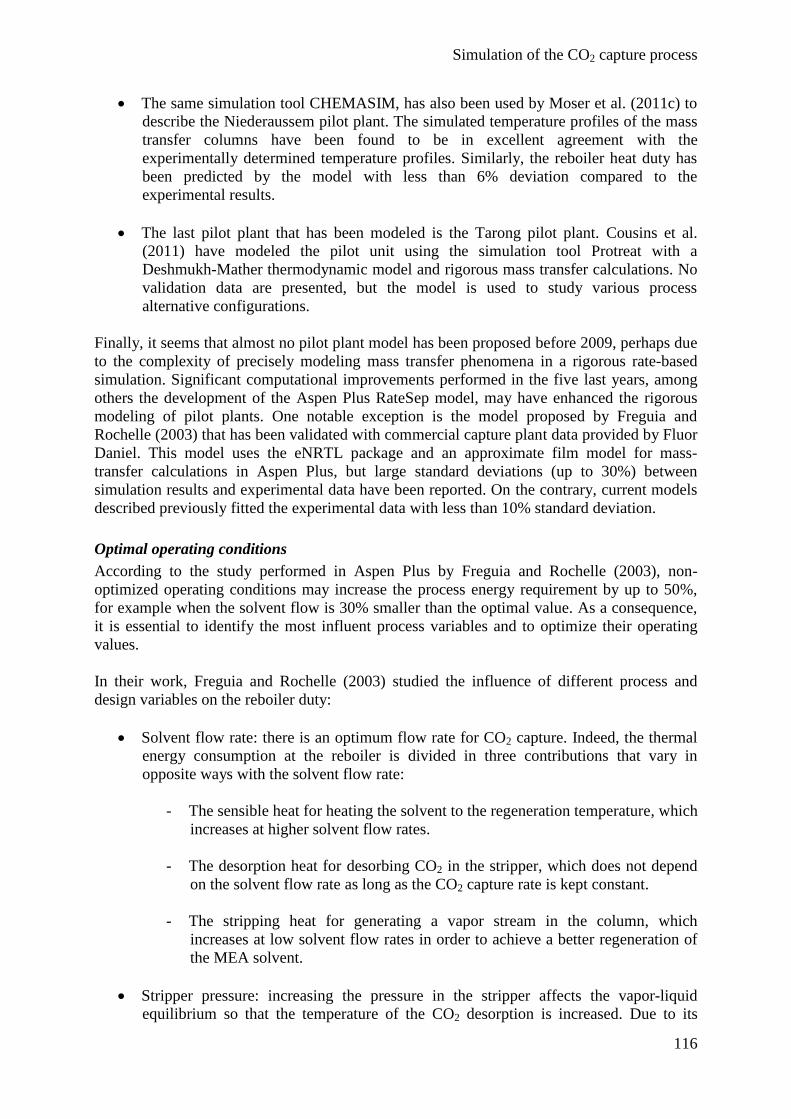
Simulation of the CO2 capture process

116

The same simulation tool CHEMASIM, has also been used by Moser et al. (2011c) to

describe the Niederaussem pilot plant. The simulated temperature profiles of the mass

transfer columns have been found to be in excellent agreement with the

experimentally determined temperature profiles. Similarly, the reboiler heat duty has

been predicted by the model with less than 6% deviation compared to the

experimental results.

The last pilot plant that has been modeled is the Tarong pilot plant. Cousins et al.

(2011) have modeled the pilot unit using the simulation tool Protreat with a

Deshmukh-Mather thermodynamic model and rigorous mass transfer calculations. No

validation data are presented, but the model is used to study various process

alternative configurations.

Finally, it seems that almost no pilot plant model has been proposed before 2009, perhaps due

to the complexity of precisely modeling mass transfer phenomena in a rigorous rate-based

simulation. Significant computational improvements performed in the five last years, among

others the development of the Aspen Plus RateSep model, may have enhanced the rigorous

modeling of pilot plants. One notable exception is the model proposed by Freguia and

Rochelle (2003) that has been validated with commercial capture plant data provided by Fluor

Daniel. This model uses the eNRTL package and an approximate film model for mass-

transfer calculations in Aspen Plus, but large standard deviations (up to 30%) between

simulation results and experimental data have been reported. On the contrary, current models

described previously fitted the experimental data with less than 10% standard deviation.

Optimal operating conditions

According to the study performed in Aspen Plus by Freguia and Rochelle (2003), non-

optimized operating conditions may increase the process energy requirement by up to 50%,

for example when the solvent flow is 30% smaller than the optimal value. As a consequence,

it is essential to identify the most influent process variables and to optimize their operating

values.

In their work, Freguia and Rochelle (2003) studied the influence of different process and

design variables on the reboiler duty:

Solvent flow rate: there is an optimum flow rate for CO2 capture. Indeed, the thermal

energy consumption at the reboiler is divided in three contributions that vary in

opposite ways with the solvent flow rate:

- The sensible heat for heating the solvent to the regeneration temperature, which

increases at higher solvent flow rates.

- The desorption heat for desorbing CO2 in the stripper, which does not depend

on the solvent flow rate as long as the CO2 capture rate is kept constant.

- The stripping heat for generating a vapor stream in the column, which

increases at low solvent flow rates in order to achieve a better regeneration of

the MEA solvent.

Stripper pressure: increasing the pressure in the stripper affects the vapor-liquid

equilibrium so that the temperature of the CO2 desorption is increased. Due to its

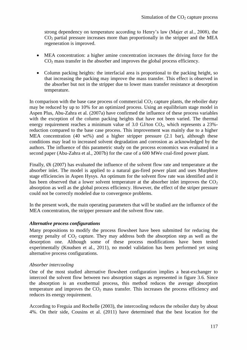
Simulation of the CO2 capture process

117

strong dependency on temperature according to Henry’s law (Majer et al., 2008), the

CO2 partial pressure increases more than proportionally in the stripper and the MEA

regeneration is improved.

MEA concentration: a higher amine concentration increases the driving force for the

CO2 mass transfer in the absorber and improves the global process efficiency.

Column packing heights: the interfacial area is proportional to the packing height, so

that increasing the packing may improve the mass transfer. This effect is observed in

the absorber but not in the stripper due to lower mass transfer resistance at desorption

temperature.

In comparison with the base case process of commercial CO2 capture plants, the reboiler duty

may be reduced by up to 10% for an optimized process. Using an equilibrium stage model in

Aspen Plus, Abu-Zahra et al. (2007a) have confirmed the influence of these process variables

with the exception of the column packing heights that have not been varied. The thermal

energy requirement reaches a minimum value of 3.0 GJ/ton CO2, which represents a 23%-

reduction compared to the base case process. This improvement was mainly due to a higher

MEA concentration (40 wt%) and a higher stripper pressure (2.1 bar), although these

conditions may lead to increased solvent degradation and corrosion as acknowledged by the

authors. The influence of this parametric study on the process economics was evaluated in a

second paper (Abu-Zahra et al., 2007b) for the case of a 600 MWe coal-fired power plant.

Finally, Øi (2007) has evaluated the influence of the solvent flow rate and temperature at the

absorber inlet. The model is applied to a natural gas-fired power plant and uses Murphree

stage efficiencies in Aspen Hysys. An optimum for the solvent flow rate was identified and it

has been observed that a lower solvent temperature at the absorber inlet improves the CO2

absorption as well as the global process efficiency. However, the effect of the striper pressure

could not be correctly modeled due to convergence problems.

In the present work, the main operating parameters that will be studied are the influence of the

MEA concentration, the stripper pressure and the solvent flow rate.

Alternative process configurations

Many propositions to modify the process flowsheet have been submitted for reducing the

energy penalty of CO2 capture. They may address both the absorption step as well as the

desorption one. Although some of these process modifications have been tested

experimentally (Knudsen et al., 2011), no model validation has been performed yet using

alternative process configurations.

Absorber intercooling

One of the most studied alternative flowsheet configuration implies a heat-exchanger to

intercool the solvent flow between two absorption stages as represented in figure 3.6. Since

the absorption is an exothermal process, this method reduces the average absorption

temperature and improves the CO2 mass transfer. This increases the process efficiency and

reduces its energy requirement.

According to Freguia and Rochelle (2003), the intercooling reduces the reboiler duty by about

4%. On their side, Cousins et al. (2011) have determined that the best location for the

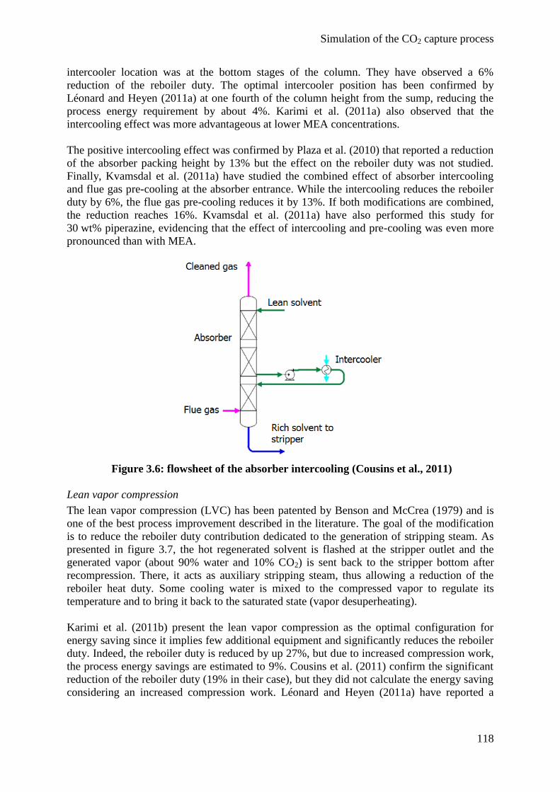
Simulation of the CO2 capture process

118

intercooler location was at the bottom stages of the column. They have observed a 6%

reduction of the reboiler duty. The optimal intercooler position has been confirmed by

Léonard and Heyen (2011a) at one fourth of the column height from the sump, reducing the

process energy requirement by about 4%. Karimi et al. (2011a) also observed that the

intercooling effect was more advantageous at lower MEA concentrations.

The positive intercooling effect was confirmed by Plaza et al. (2010) that reported a reduction

of the absorber packing height by 13% but the effect on the reboiler duty was not studied.

Finally, Kvamsdal et al. (2011a) have studied the combined effect of absorber intercooling

and flue gas pre-cooling at the absorber entrance. While the intercooling reduces the reboiler

duty by 6%, the flue gas pre-cooling reduces it by 13%. If both modifications are combined,

the reduction reaches 16%. Kvamsdal et al. (2011a) have also performed this study for

30 wt% piperazine, evidencing that the effect of intercooling and pre-cooling was even more

pronounced than with MEA.

Figure 3.6: flowsheet of the absorber intercooling (Cousins et al., 2011)

Lean vapor compression

The lean vapor compression (LVC) has been patented by Benson and McCrea (1979) and is

one of the best process improvement described in the literature. The goal of the modification

is to reduce the reboiler duty contribution dedicated to the generation of stripping steam. As

presented in figure 3.7, the hot regenerated solvent is flashed at the stripper outlet and the

generated vapor (about 90% water and 10% CO2) is sent back to the stripper bottom after

recompression. There, it acts as auxiliary stripping steam, thus allowing a reduction of the

reboiler heat duty. Some cooling water is mixed to the compressed vapor to regulate its

temperature and to bring it back to the saturated state (vapor desuperheating).

Karimi et al. (2011b) present the lean vapor compression as the optimal configuration for

energy saving since it implies few additional equipment and significantly reduces the reboiler

duty. Indeed, the reboiler duty is reduced by up 27%, but due to increased compression work,

the process energy savings are estimated to 9%. Cousins et al. (2011) confirm the significant

reduction of the reboiler duty (19% in their case), but they did not calculate the energy saving

considering an increased compression work. Léonard and Heyen (2011a) have reported a

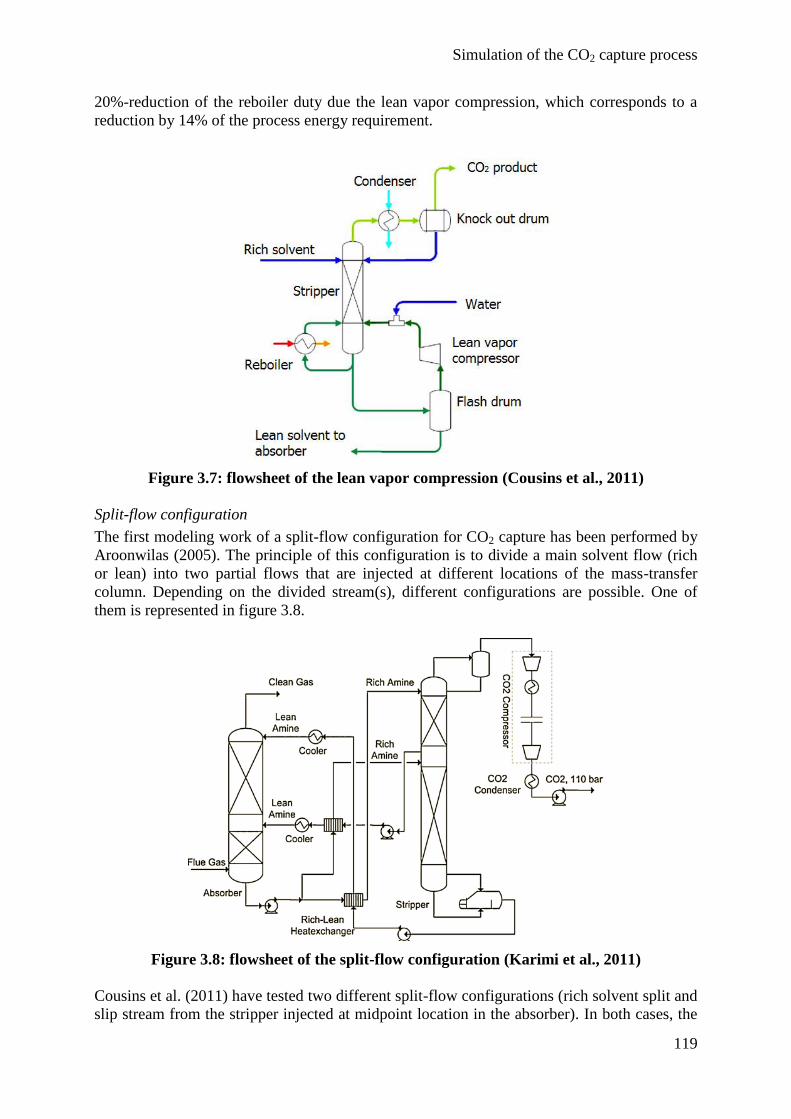
Simulation of the CO2 capture process

119

20%-reduction of the reboiler duty due the lean vapor compression, which corresponds to a

reduction by 14% of the process energy requirement.

Figure 3.7: flowsheet of the lean vapor compression (Cousins et al., 2011)

Split-flow configuration

The first modeling work of a split-flow configuration for CO2 capture has been performed by

Aroonwilas (2005). The principle of this configuration is to divide a main solvent flow (rich

or lean) into two partial flows that are injected at different locations of the mass-transfer

column. Depending on the divided stream(s), different configurations are possible. One of

them is represented in figure 3.8.

Figure 3.8: flowsheet of the split-flow configuration (Karimi et al., 2011)

Cousins et al. (2011) have tested two different split-flow configurations (rich solvent split and

slip stream from the stripper injected at midpoint location in the absorber). In both cases, the

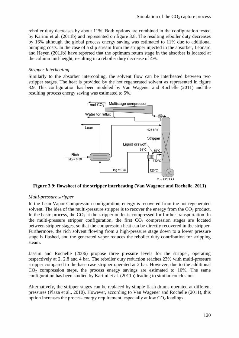
Simulation of the CO2 capture process

120

reboiler duty decreases by about 11%. Both options are combined in the configuration tested

by Karimi et al. (2011b) and represented on figure 3.8. The resulting reboiler duty decreases

by 16% although the global process energy saving was estimated to 11% due to additional

pumping costs. In the case of a slip stream from the stripper injected in the absorber, Léonard

and Heyen (2011b) have reported that the optimum return stage in the absorber is located at

the column mid-height, resulting in a reboiler duty decrease of 4%.

Stripper Interheating

Similarly to the absorber intercooling, the solvent flow can be interheated between two

stripper stages. The heat is provided by the hot regenerated solvent as represented in figure

3.9. This configuration has been modeled by Van Wagener and Rochelle (2011) and the

resulting process energy saving was estimated to 5%.

Figure 3.9: flowsheet of the stripper interheating (Van Wagener and Rochelle, 2011)

Multi-pressure stripper

In the Lean Vapor Compression configuration, energy is recovered from the hot regenerated

solvent. The idea of the multi-pressure stripper is to recover the energy from the CO2 product.

In the basic process, the CO2 at the stripper outlet is compressed for further transportation. In

the multi-pressure stripper configuration, the first CO2 compression stages are located

between stripper stages, so that the compression heat can be directly recovered in the stripper.

Furthermore, the rich solvent flowing from a high-pressure stage down to a lower pressure

stage is flashed, and the generated vapor reduces the reboiler duty contribution for stripping

steam.

Jassim and Rochelle (2006) propose three pressure levels for the stripper, operating

respectively at 2, 2.8 and 4 bar. The reboiler duty reduction reaches 23% with multi-pressure

stripper compared to the base case stripper operated at 2 bar. However, due to the additional

CO2 compression steps, the process energy savings are estimated to 10%. The same

configuration has been studied by Karimi et al. (2011b) leading to similar conclusions.

Alternatively, the stripper stages can be replaced by simple flash drums operated at different

pressures (Plaza et al., 2010). However, according to Van Wagener and Rochelle (2011), this

option increases the process energy requirement, especially at low CO2 loadings.

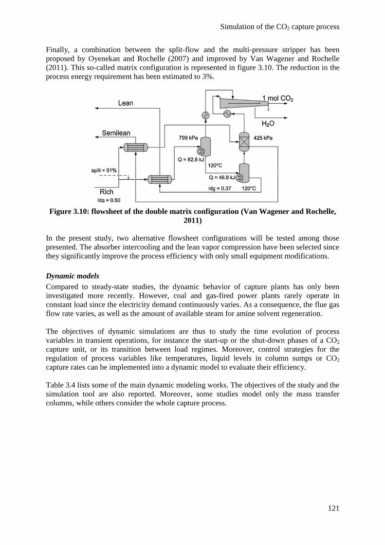
Simulation of the CO2 capture process

121

Finally, a combination between the split-flow and the multi-pressure stripper has been

proposed by Oyenekan and Rochelle (2007) and improved by Van Wagener and Rochelle

(2011). This so-called matrix configuration is represented in figure 3.10. The reduction in the

process energy requirement has been estimated to 3%.

Figure 3.10: flowsheet of the double matrix configuration (Van Wagener and Rochelle,

2011)

In the present study, two alternative flowsheet configurations will be tested among those

presented. The absorber intercooling and the lean vapor compression have been selected since

they significantly improve the process efficiency with only small equipment modifications.

Dynamic models

Compared to steady-state studies, the dynamic behavior of capture plants has only been

investigated more recently. However, coal and gas-fired power plants rarely operate in

constant load since the electricity demand continuously varies. As a consequence, the flue gas

flow rate varies, as well as the amount of available steam for amine solvent regeneration.

The objectives of dynamic simulations are thus to study the time evolution of process

variables in transient operations, for instance the start-up or the shut-down phases of a CO2

capture unit, or its transition between load regimes. Moreover, control strategies for the

regulation of process variables like temperatures, liquid levels in column sumps or CO2

capture rates can be implemented into a dynamic model to evaluate their efficiency.

Table 3.4 lists some of the main dynamic modeling works. The objectives of the study and the

simulation tool are also reported. Moreover, some studies model only the mass transfer

columns, while others consider the whole capture process.

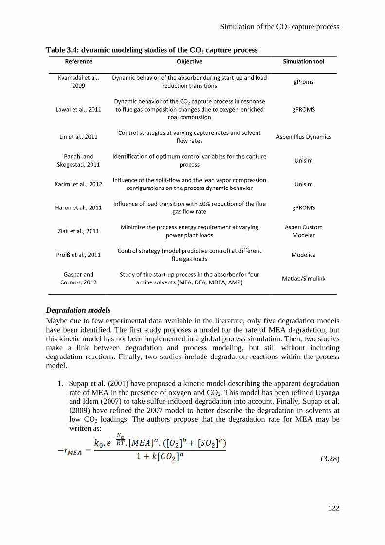
Simulation of the CO2 capture process

122

Table 3.4: dynamic modeling studies of the CO2 capture process

Reference Objective Simulation tool

Kvamsdal et al., 2009

Dynamic behavior of the absorber during start-up and load reduction transitions

gProms

Lawal et al., 2011 Dynamic behavior of the CO2 capture process in response to flue gas composition changes due to oxygen-enriched

coal combustion gPROMS

Lin et al., 2011 Control strategies at varying capture rates and solvent

flow rates Aspen Plus Dynamics

Panahi and Skogestad, 2011

Identification of optimum control variables for the capture process

Unisim

Karimi et al., 2012 Influence of the split-flow and the lean vapor compression

configurations on the process dynamic behavior Unisim

Harun et al., 2011 Influence of load transition with 50% reduction of the flue

gas flow rate gPROMS

Ziaii et al., 2011 Minimize the process energy requirement at varying

power plant loads Aspen Custom

Modeler

Prölß et al., 2011 Control strategy (model predictive control) at different

flue gas loads Modelica

Gaspar and Cormos, 2012

Study of the start-up process in the absorber for four amine solvents (MEA, DEA, MDEA, AMP)

Matlab/Simulink

Degradation models

Maybe due to few experimental data available in the literature, only five degradation models

have been identified. The first study proposes a model for the rate of MEA degradation, but

this kinetic model has not been implemented in a global process simulation. Then, two studies

make a link between degradation and process modeling, but still without including

degradation reactions. Finally, two studies include degradation reactions within the process

model.

1. Supap et al. (2001) have proposed a kinetic model describing the apparent degradation

rate of MEA in the presence of oxygen and CO2. This model has been refined Uyanga

and Idem (2007) to take sulfur-induced degradation into account. Finally, Supap et al.

(2009) have refined the 2007 model to better describe the degradation in solvents at

low CO2 loadings. The authors propose that the degradation rate for MEA may be

written as:

(3.28)

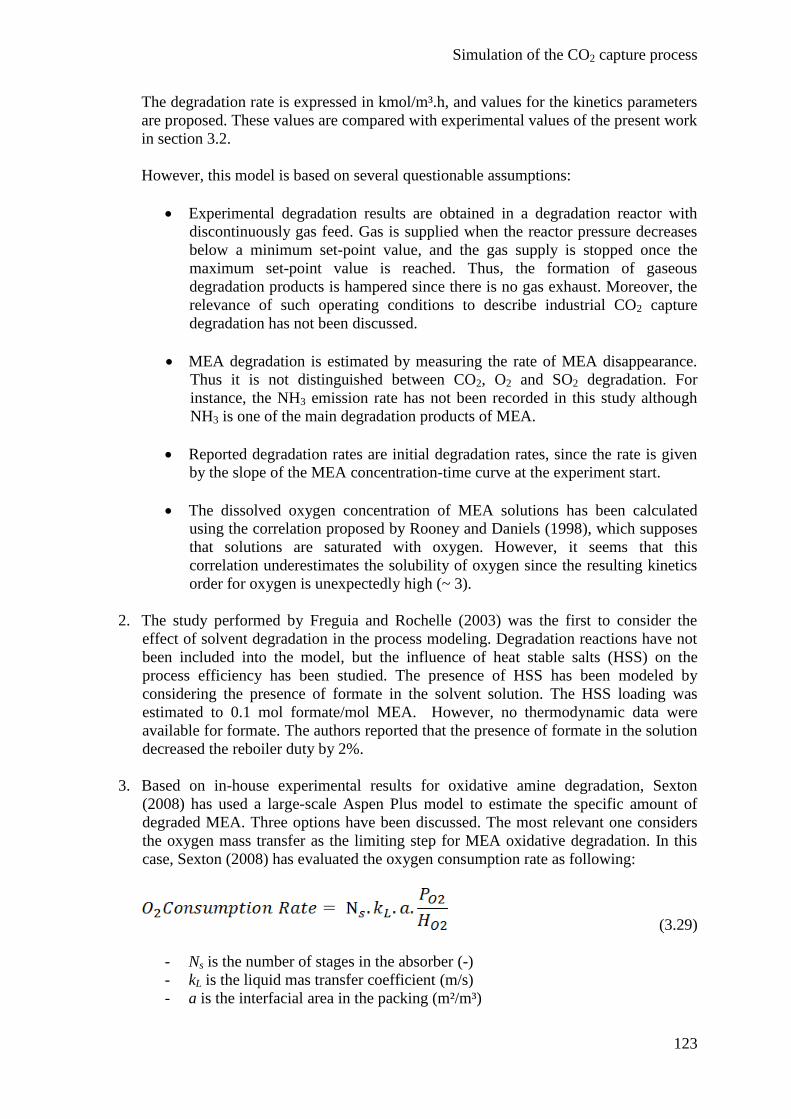
Simulation of the CO2 capture process

123

The degradation rate is expressed in kmol/m³.h, and values for the kinetics parameters

are proposed. These values are compared with experimental values of the present work

in section 3.2.

However, this model is based on several questionable assumptions:

Experimental degradation results are obtained in a degradation reactor with

discontinuously gas feed. Gas is supplied when the reactor pressure decreases

below a minimum set-point value, and the gas supply is stopped once the

maximum set-point value is reached. Thus, the formation of gaseous

degradation products is hampered since there is no gas exhaust. Moreover, the

relevance of such operating conditions to describe industrial CO2 capture

degradation has not been discussed.

MEA degradation is estimated by measuring the rate of MEA disappearance.

Thus it is not distinguished between CO2, O2 and SO2 degradation. For

instance, the NH3 emission rate has not been recorded in this study although

NH3 is one of the main degradation products of MEA.

Reported degradation rates are initial degradation rates, since the rate is given

by the slope of the MEA concentration-time curve at the experiment start.

The dissolved oxygen concentration of MEA solutions has been calculated

using the correlation proposed by Rooney and Daniels (1998), which supposes

that solutions are saturated with oxygen. However, it seems that this

correlation underestimates the solubility of oxygen since the resulting kinetics

order for oxygen is unexpectedly high (~ 3).

2. The study performed by Freguia and Rochelle (2003) was the first to consider the

effect of solvent degradation in the process modeling. Degradation reactions have not

been included into the model, but the influence of heat stable salts (HSS) on the

process efficiency has been studied. The presence of HSS has been modeled by

considering the presence of formate in the solvent solution. The HSS loading was

estimated to 0.1 mol formate/mol MEA. However, no thermodynamic data were

available for formate. The authors reported that the presence of formate in the solution

decreased the reboiler duty by 2%.

3. Based on in-house experimental results for oxidative amine degradation, Sexton

(2008) has used a large-scale Aspen Plus model to estimate the specific amount of

degraded MEA. Three options have been discussed. The most relevant one considers

the oxygen mass transfer as the limiting step for MEA oxidative degradation. In this

case, Sexton (2008) has evaluated the oxygen consumption rate as following:

(3.29)

- Ns is the number of stages in the absorber (-)

- kL is the liquid mas transfer coefficient (m/s)

- a is the interfacial area in the packing (m²/m³)

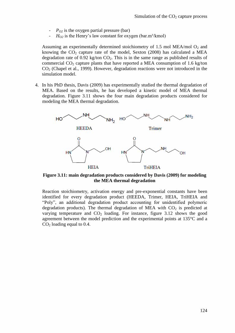
Simulation of the CO2 capture process

124

- PO2 is the oxygen partial pressure (bar)

- HO2 is the Henry’s law constant for oxygen (bar.m³/kmol)

Assuming an experimentally determined stoichiometry of 1.5 mol MEA/mol O2 and

knowing the CO2 capture rate of the model, Sexton (2008) has calculated a MEA

degradation rate of 0.92 kg/ton CO2. This is in the same range as published results of

commercial CO2 capture plants that have reported a MEA consumption of 1.6 kg/ton

CO2 (Chapel et al., 1999). However, degradation reactions were not introduced in the

simulation model.

4. In his PhD thesis, Davis (2009) has experimentally studied the thermal degradation of

MEA. Based on the results, he has developed a kinetic model of MEA thermal

degradation. Figure 3.11 shows the four main degradation products considered for

modeling the MEA thermal degradation.

Figure 3.11: main degradation products considered by Davis (2009) for modeling

the MEA thermal degradation

Reaction stoichiometry, activation energy and pre-exponential constants have been

identified for every degradation product (HEEDA, Trimer, HEIA, TriHEIA and

“Poly”, an additional degradation product accounting for unidentified polymeric

degradation products). The thermal degradation of MEA with CO2 is predicted at

varying temperature and CO2 loading. For instance, figure 3.12 shows the good

agreement between the model prediction and the experimental points at 135°C and a

CO2 loading equal to 0.4.

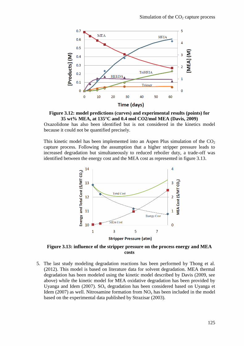
Simulation of the CO2 capture process

125

Figure 3.12: model predictions (curves) and experimental results (points) for

35 wt% MEA, at 135°C and 0.4 mol CO2/mol MEA (Davis, 2009)

Oxazolidone has also been identified but is not considered in the kinetics model

because it could not be quantified precisely.

This kinetic model has been implemented into an Aspen Plus simulation of the CO2

capture process. Following the assumption that a higher stripper pressure leads to

increased degradation but simultaneously to reduced reboiler duty, a trade-off was

identified between the energy cost and the MEA cost as represented in figure 3.13.

Figure 3.13: influence of the stripper pressure on the process energy and MEA

costs

5. The last study modeling degradation reactions has been performed by Thong et al.

(2012). This model is based on literature data for solvent degradation. MEA thermal

degradation has been modeled using the kinetic model described by Davis (2009, see

above) while the kinetic model for MEA oxidative degradation has been provided by

Uyanga and Idem (2007). SOx degradation has been considered based on Uyanga et

Idem (2007) as well. Nitrosamine formation from NOx has been included in the model

based on the experimental data published by Strazisar (2003).

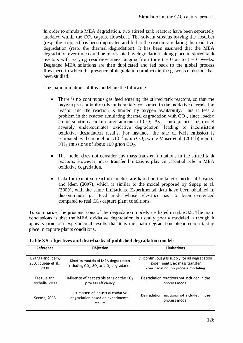
Simulation of the CO2 capture process

126

In order to simulate MEA degradation, two stirred tank reactors have been separately

modeled within the CO2 capture flowsheet. The solvent streams leaving the absorber

(resp. the stripper) has been duplicated and fed to the reactor simulating the oxidative

degradation (resp. the thermal degradation). It has been assumed that the MEA

degradation over time could be represented by degradation taking place in stirred tank

reactors with varying residence times ranging from time t = 0 up to t = 6 weeks.

Degraded MEA solutions are then duplicated and fed back to the global process

flowsheet, in which the presence of degradation products in the gaseous emissions has

been studied.

The main limitations of this model are the following:

There is no continuous gas feed entering the stirred tank reactors, so that the

oxygen present in the solvent is rapidly consumed in the oxidative degradation

reactor and the reaction is limited by oxygen availability. This is less a

problem in the reactor simulating thermal degradation with CO2, since loaded

amine solutions contain large amounts of CO2. As a consequence, this model

severely underestimates oxidative degradation, leading to inconsistent

oxidative degradation results. For instance, the rate of NH3 emission is

estimated by the model to 1.10-10

g/ton CO2, while Moser et al. (2011b) reports

NH3 emissions of about 100 g/ton CO2.

The model does not consider any mass transfer limitations in the stirred tank

reactors. However, mass transfer limitations play an essential role in MEA

oxidative degradation.

Data for oxidative reaction kinetics are based on the kinetic model of Uyanga

and Idem (2007), which is similar to the model proposed by Supap et al.

(2009), with the same limitations. Experimental data have been obtained in

discontinuous gas feed mode whose relevance has not been evidenced

compared to real CO2 capture plant conditions.

To summarize, the pros and cons of the degradation models are listed in table 3.5. The main

conclusions is that the MEA oxidative degradation is usually poorly modeled, although it

appears from our experimental results that it is the main degradation phenomenon taking

place in capture plants conditions.

Table 3.5: objectives and drawbacks of published degradation models

Reference Objective Limitations

Uyanga and Idem, 2007; Supap et al.,

2009

Kinetics models of MEA degradation including CO2, SO2 and O2 degradation

Discontinuous gas supply for all degradation experiments, no mass transfer

consideration, no process modeling

Freguia and Rochelle, 2003

Influence of heat stable salts on the CO2 process efficiency

Degradation reactions not included in the process model

Sexton, 2008 Estimation of industrial oxidative

degradation based on experimental results

Degradation reactions not included in the process model

Simulation of the CO2 capture process

127

Davis, 2009 Detailed reaction modeling of thermal

degradation based on in-house experimental data

Oxidative degradation not considered

Thong et al., 2012 Complete degradation overview

(oxidative, thermal with CO2, SOx and NOx)

Based on experimental data from Uyanga and Idem (2007) for O2 and SO2 degradation, few experimental data for NOx degradation

Simulation of the CO2 capture process

128

3. Model construction

In this section, the models developed for studying the CO2 capture process are described.

Design data from two different pilot units have been considered:

A Mobile Pilot Unit (MPU) treating a flue gas load of 2500 Nm³/h.

The Esbjerg Pilot Plant (EPP) treating a flue gas load of 5000 Nm³/h.

It is important to note that no rigorous model validation has been performed. First, it is not the

objective of this work to precisely describe a pilot capture plant, but rather to propose new

modeling pathway including degradation phenomena. Then, the relevance of simulation

studies compared to experimental results has been demonstrated in section 2.3. Finally,

precise design data are sometimes missing, so that the models developed in this work often

combine design data from the Esbjerg Pilot Plant with data from the Mobile Pilot Unit.

All the models developed in this work simulate a carbon capture process with flue gas from a

coal-fired power plant. The solvent used for the reactive absorption is an aqueous solution of

30 wt% monoethanolamine (MEA) and the process is designed to capture 90% of the CO2

feed. Steady-state models have been developed using the software Aspen Plus (versions 7.0,

7.2 and 8.0), while Aspen Plus Dynamics (version 7.3) has been used for unsteady-state

simulations. All simulations have been performed using the electrolyte NRTL activity

coefficient model, with the Redlich-Kwong equation of state for vapor phase calculations.

Different modeling approaches have been considered, leading to four distinct models:

The equilibrium model is a first approach to simulate the steady-state process of CO2

capture. It is based on the assumption of equilibrium stages for the mass transfer

columns, so that heat and mass transfer limitations are neglected. Moreover, chemical

kinetics limitations are neglected as well.

The rate-based model also simulates the steady-state process but rigorously calculates

the mass transfer in the columns. Furthermore, the chemical kinetics limitations are

considered in this model.

The dynamic model has been developed to study the dynamic behavior of the CO2

capture process. It is based on the assumption of equilibrium stages and chemical

kinetics limitations are not considered.

Finally, the degradation model simulates the CO2 capture process with consideration

of degradation reactions. Mass transfer and chemical kinetics limitations are

considered. Moreover, the modeling of degradation reactions is based on the

experimental results for MEA oxidative and thermal degradation with CO2 described

in Chapter II.

The first two models have been evaluated based on a flue gas load of 2500 Nm³/h, so that they

are referred to as MPU models, even if some missing design data have been retrieved from

the Esbjerg Pilot Plant. The dynamic and the degradation models consider a flue gas load of

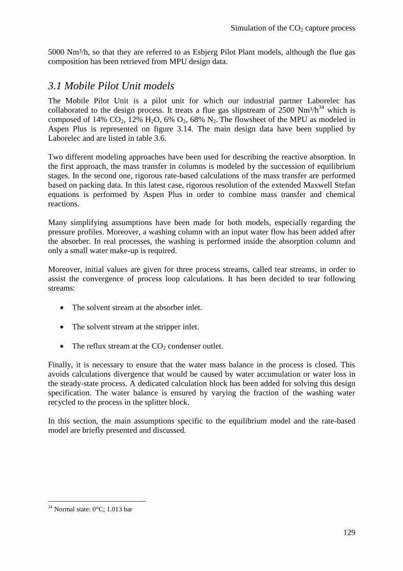
Simulation of the CO2 capture process

129

5000 Nm³/h, so that they are referred to as Esbjerg Pilot Plant models, although the flue gas

composition has been retrieved from MPU design data.

3.1 Mobile Pilot Unit models

The Mobile Pilot Unit is a pilot unit for which our industrial partner Laborelec has

collaborated to the design process. It treats a flue gas slipstream of 2500 Nm³/h34

which is

composed of 14% CO2, 12% H2O, 6% O2, 68% N2. The flowsheet of the MPU as modeled in

Aspen Plus is represented on figure 3.14. The main design data have been supplied by

Laborelec and are listed in table 3.6.

Two different modeling approaches have been used for describing the reactive absorption. In

the first approach, the mass transfer in columns is modeled by the succession of equilibrium

stages. In the second one, rigorous rate-based calculations of the mass transfer are performed

based on packing data. In this latest case, rigorous resolution of the extended Maxwell Stefan

equations is performed by Aspen Plus in order to combine mass transfer and chemical

reactions.

Many simplifying assumptions have been made for both models, especially regarding the

pressure profiles. Moreover, a washing column with an input water flow has been added after

the absorber. In real processes, the washing is performed inside the absorption column and

only a small water make-up is required.

Moreover, initial values are given for three process streams, called tear streams, in order to

assist the convergence of process loop calculations. It has been decided to tear following

streams:

The solvent stream at the absorber inlet.

The solvent stream at the stripper inlet.

The reflux stream at the CO2 condenser outlet.

Finally, it is necessary to ensure that the water mass balance in the process is closed. This

avoids calculations divergence that would be caused by water accumulation or water loss in

the steady-state process. A dedicated calculation block has been added for solving this design

specification. The water balance is ensured by varying the fraction of the washing water

recycled to the process in the splitter block.

In this section, the main assumptions specific to the equilibrium model and the rate-based

model are briefly presented and discussed.

34

Normal state: 0°C; 1.013 bar

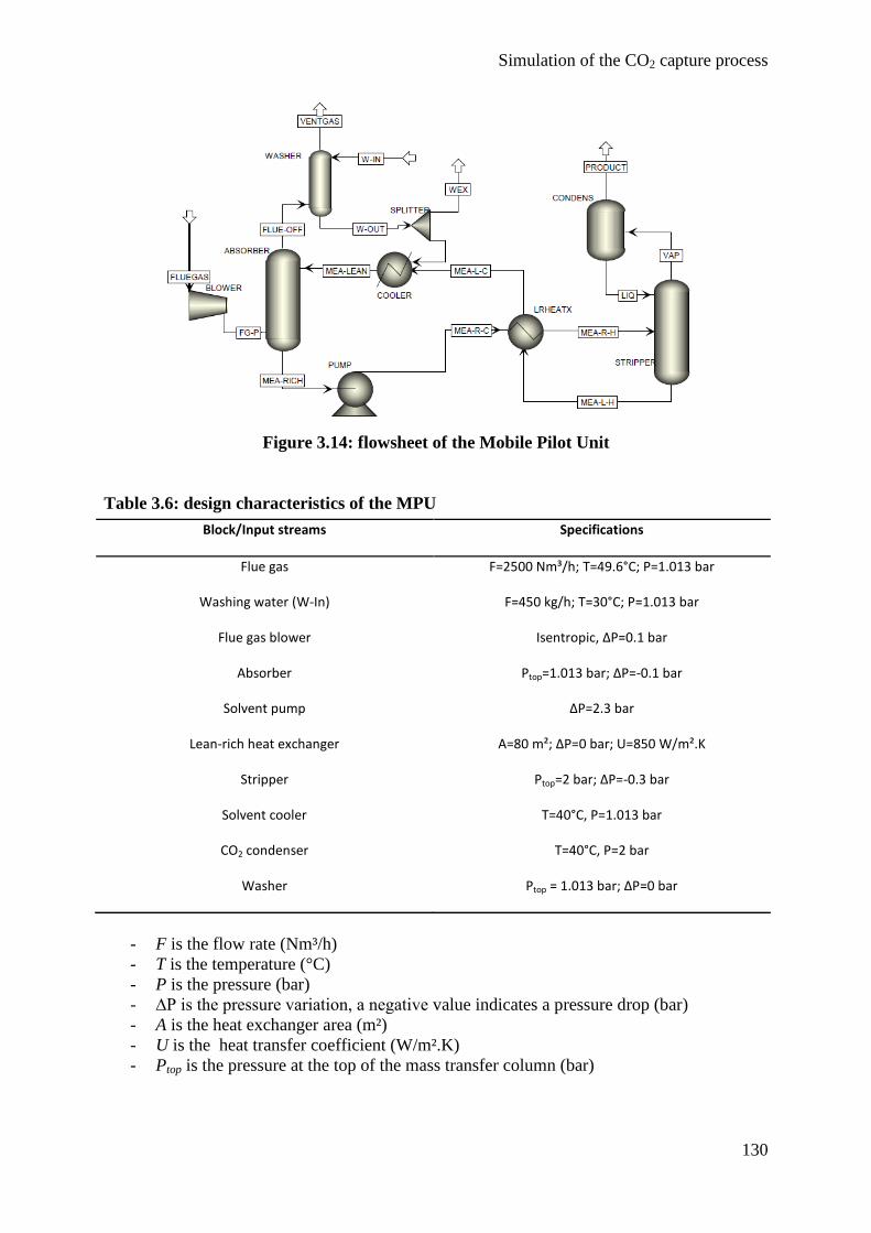
Simulation of the CO2 capture process

130

Figure 3.14: flowsheet of the Mobile Pilot Unit

Table 3.6: design characteristics of the MPU

Block/Input streams Specifications

Flue gas F=2500 Nm³/h; T=49.6°C; P=1.013 bar

Washing water (W-In) F=450 kg/h; T=30°C; P=1.013 bar

Flue gas blower Isentropic, ∆P=0.1 bar

Absorber Ptop=1.013 bar; ∆P=-0.1 bar

Solvent pump ∆P=2.3 bar

Lean-rich heat exchanger A=80 m²; ∆P=0 bar; U=850 W/m².K

Stripper Ptop=2 bar; ∆P=-0.3 bar

Solvent cooler T=40°C, P=1.013 bar

CO2 condenser T=40°C, P=2 bar

Washer Ptop = 1.013 bar; ∆P=0 bar

- F is the flow rate (Nm³/h)

- T is the temperature (°C)

- P is the pressure (bar)

- ∆P is the pressure variation, a negative value indicates a pressure drop (bar)

- A is the heat exchanger area (m²)

- U is the heat transfer coefficient (W/m².K)

- Ptop is the pressure at the top of the mass transfer column (bar)

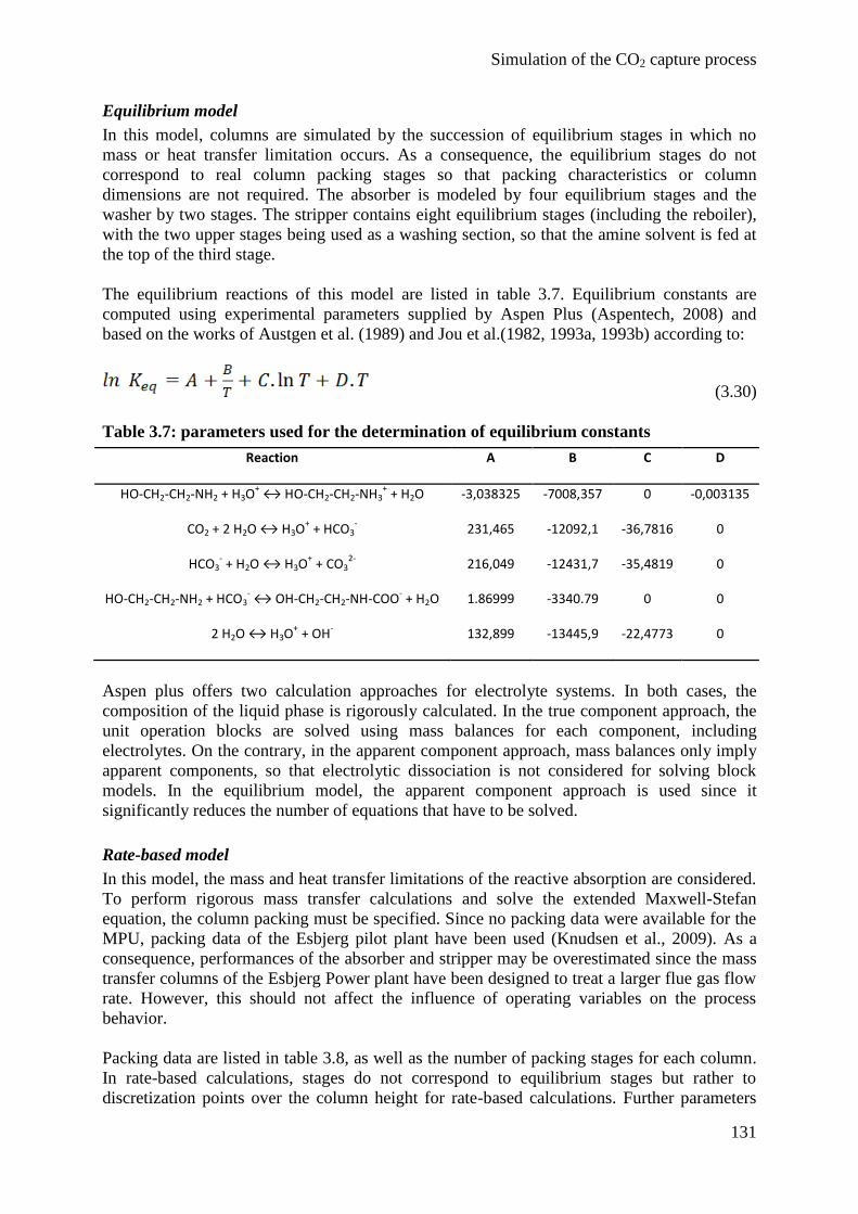
Simulation of the CO2 capture process

131

Equilibrium model

In this model, columns are simulated by the succession of equilibrium stages in which no

mass or heat transfer limitation occurs. As a consequence, the equilibrium stages do not

correspond to real column packing stages so that packing characteristics or column

dimensions are not required. The absorber is modeled by four equilibrium stages and the

washer by two stages. The stripper contains eight equilibrium stages (including the reboiler),

with the two upper stages being used as a washing section, so that the amine solvent is fed at

the top of the third stage.

The equilibrium reactions of this model are listed in table 3.7. Equilibrium constants are

computed using experimental parameters supplied by Aspen Plus (Aspentech, 2008) and

based on the works of Austgen et al. (1989) and Jou et al.(1982, 1993a, 1993b) according to:

(3.30)

Table 3.7: parameters used for the determination of equilibrium constants

Reaction A B C D

HO-CH2-CH2-NH2 + H3O+ ↔ HO-CH2-CH2-NH3

+ + H2O -3,038325 -7008,357 0 -0,003135

CO2 + 2 H2O ↔ H3O+ + HCO3

- 231,465 -12092,1 -36,7816 0

HCO3- + H2O ↔ H3O

+ + CO3

2- 216,049 -12431,7 -35,4819 0

HO-CH2-CH2-NH2 + HCO3- ↔ OH-CH2-CH2-NH-COO

- + H2O 1.86999 -3340.79 0 0

2 H2O ↔ H3O+ + OH

- 132,899 -13445,9 -22,4773 0

Aspen plus offers two calculation approaches for electrolyte systems. In both cases, the

composition of the liquid phase is rigorously calculated. In the true component approach, the

unit operation blocks are solved using mass balances for each component, including

electrolytes. On the contrary, in the apparent component approach, mass balances only imply

apparent components, so that electrolytic dissociation is not considered for solving block

models. In the equilibrium model, the apparent component approach is used since it

significantly reduces the number of equations that have to be solved.

Rate-based model

In this model, the mass and heat transfer limitations of the reactive absorption are considered.

To perform rigorous mass transfer calculations and solve the extended Maxwell-Stefan

equation, the column packing must be specified. Since no packing data were available for the

MPU, packing data of the Esbjerg pilot plant have been used (Knudsen et al., 2009). As a

consequence, performances of the absorber and stripper may be overestimated since the mass

transfer columns of the Esbjerg Power plant have been designed to treat a larger flue gas flow

rate. However, this should not affect the influence of operating variables on the process

behavior.

Packing data are listed in table 3.8, as well as the number of packing stages for each column.

In rate-based calculations, stages do not correspond to equilibrium stages but rather to

discretization points over the column height for rate-based calculations. Further parameters

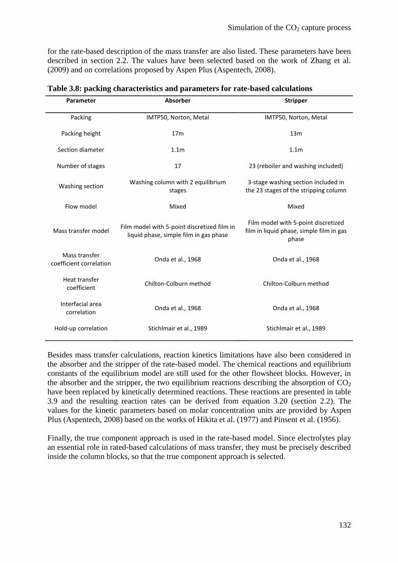
Simulation of the CO2 capture process

132

for the rate-based description of the mass transfer are also listed. These parameters have been

described in section 2.2. The values have been selected based on the work of Zhang et al.

(2009) and on correlations proposed by Aspen Plus (Aspentech, 2008).

Table 3.8: packing characteristics and parameters for rate-based calculations

Parameter Absorber Stripper

Packing IMTP50, Norton, Metal IMTP50, Norton, Metal

Packing height 17m 13m

Section diameter 1.1m 1.1m

Number of stages 17 23 (reboiler and washing included)

Washing section Washing column with 2 equilibrium

stages 3-stage washing section included in

the 23 stages of the stripping column

Flow model

Mixed Mixed

Mass transfer model Film model with 5-point discretized film in

liquid phase, simple film in gas phase

Film model with 5-point discretized film in liquid phase, simple film in gas

phase

Mass transfer coefficient correlation

Onda et al., 1968 Onda et al., 1968

Heat transfer coefficient

Chilton-Colburn method Chilton-Colburn method

Interfacial area correlation

Onda et al., 1968 Onda et al., 1968

Hold-up correlation Stichlmair et al., 1989 Stichlmair et al., 1989

Besides mass transfer calculations, reaction kinetics limitations have also been considered in

the absorber and the stripper of the rate-based model. The chemical reactions and equilibrium

constants of the equilibrium model are still used for the other flowsheet blocks. However, in

the absorber and the stripper, the two equilibrium reactions describing the absorption of CO2

have been replaced by kinetically determined reactions. These reactions are presented in table

3.9 and the resulting reaction rates can be derived from equation 3.20 (section 2.2). The

values for the kinetic parameters based on molar concentration units are provided by Aspen

Plus (Aspentech, 2008) based on the works of Hikita et al. (1977) and Pinsent et al. (1956).

Finally, the true component approach is used in the rate-based model. Since electrolytes play

an essential role in rated-based calculations of mass transfer, they must be precisely described

inside the column blocks, so that the true component approach is selected.

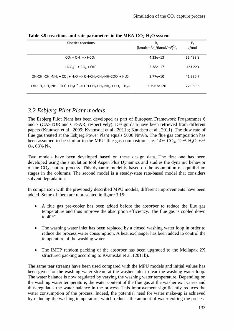
Simulation of the CO2 capture process

133

Table 3.9: reactions and rate parameters in the MEA-CO2-H2O system

Kinetics reactions k0 (kmol/m³.s)/(kmol/m³)

∑αi

Ea J/mol

CO2 + OH- --> HCO3

- 4.32e+13 55 433.8

HCO3- --> CO2 + OH

- 2.38e+17 123 223

OH-CH2-CH2-NH2 + CO2 + H2O --> OH-CH2-CH2-NH-COO- + H3O

+ 9.77e+10 41 236.7

OH-CH2-CH2-NH-COO- + H3O

+ --> OH-CH2-CH2-NH2 + CO2 + H2O 2.7963e+20 72 089.5

3.2 Esbjerg Pilot Plant models

The Esbjerg Pilot Plant has been developed as part of European Framework Programmes 6

and 7 (CASTOR and CESAR, respectively). Design data have been retrieved from different

papers (Knudsen et al., 2009; Kvamsdal et al., 2011b; Knudsen et al., 2011). The flow rate of

flue gas treated at the Esbjerg Power Plant equals 5000 Nm³/h. The flue gas composition has

been assumed to be similar to the MPU flue gas composition, i.e. 14% CO2, 12% H2O, 6%

O2, 68% N2.

Two models have been developed based on these design data. The first one has been

developed using the simulation tool Aspen Plus Dynamics and studies the dynamic behavior

of the CO2 capture process. This dynamic model is based on the assumption of equilibrium

stages in the columns. The second model is a steady-state rate-based model that considers

solvent degradation.

In comparison with the previously described MPU models, different improvements have been

added. Some of them are represented in figure 3.15:

A flue gas pre-cooler has been added before the absorber to reduce the flue gas

temperature and thus improve the absorption efficiency. The flue gas is cooled down

to 40°C.

The washing water inlet has been replaced by a closed washing water loop in order to

reduce the process water consumption. A heat exchanger has been added to control the

temperature of the washing water.

The IMTP random packing of the absorber has been upgraded to the Mellapak 2X

structured packing according to Kvamsdal et al. (2011b).

The same tear streams have been used compared with the MPU models and initial values has

been given for the washing water stream at the washer inlet to tear the washing water loop.

The water balance is now regulated by varying the washing water temperature. Depending on

the washing water temperature, the water content of the flue gas at the washer exit varies and

thus regulates the water balance in the process. This improvement significantly reduces the

water consumption of the process. Indeed, the potential need for water make-up is achieved

by reducing the washing temperature, which reduces the amount of water exiting the process

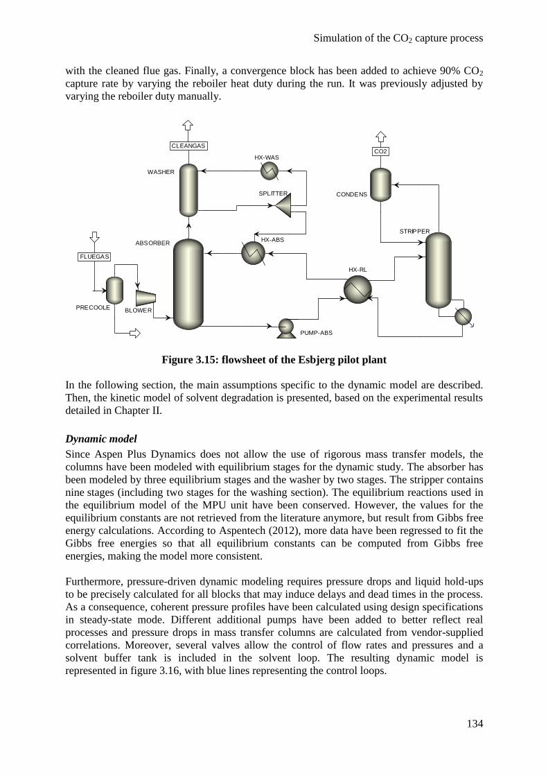
Simulation of the CO2 capture process

134

with the cleaned flue gas. Finally, a convergence block has been added to achieve 90% CO2

capture rate by varying the reboiler heat duty during the run. It was previously adjusted by

varying the reboiler duty manually.

ABSORBER

PUMP-ABS

WASHER

STRIPPER

CONDENS

HX-RL

SPLITTER

BLOWERPRECOOLE

HX-WAS

HX-ABS

CLEANGAS

CO2

FLUEGAS

Figure 3.15: flowsheet of the Esbjerg pilot plant

In the following section, the main assumptions specific to the dynamic model are described.

Then, the kinetic model of solvent degradation is presented, based on the experimental results

detailed in Chapter II.

Dynamic model

Since Aspen Plus Dynamics does not allow the use of rigorous mass transfer models, the

columns have been modeled with equilibrium stages for the dynamic study. The absorber has

been modeled by three equilibrium stages and the washer by two stages. The stripper contains

nine stages (including two stages for the washing section). The equilibrium reactions used in

the equilibrium model of the MPU unit have been conserved. However, the values for the

equilibrium constants are not retrieved from the literature anymore, but result from Gibbs free

energy calculations. According to Aspentech (2012), more data have been regressed to fit the

Gibbs free energies so that all equilibrium constants can be computed from Gibbs free

energies, making the model more consistent.

Furthermore, pressure-driven dynamic modeling requires pressure drops and liquid hold-ups

to be precisely calculated for all blocks that may induce delays and dead times in the process.

As a consequence, coherent pressure profiles have been calculated using design specifications

in steady-state mode. Different additional pumps have been added to better reflect real

processes and pressure drops in mass transfer columns are calculated from vendor-supplied

correlations. Moreover, several valves allow the control of flow rates and pressures and a

solvent buffer tank is included in the solvent loop. The resulting dynamic model is

represented in figure 3.16, with blue lines representing the control loops.

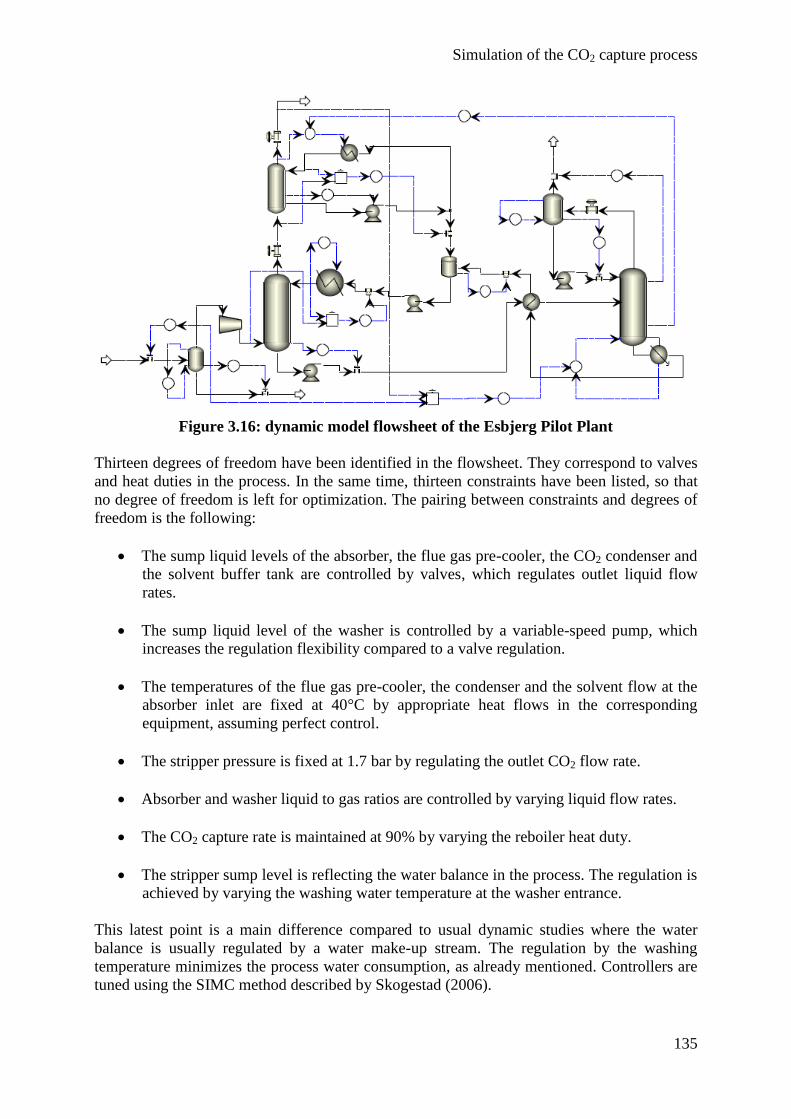
Simulation of the CO2 capture process

135

Figure 3.16: dynamic model flowsheet of the Esbjerg Pilot Plant

Thirteen degrees of freedom have been identified in the flowsheet. They correspond to valves

and heat duties in the process. In the same time, thirteen constraints have been listed, so that

no degree of freedom is left for optimization. The pairing between constraints and degrees of

freedom is the following:

The sump liquid levels of the absorber, the flue gas pre-cooler, the CO2 condenser and

the solvent buffer tank are controlled by valves, which regulates outlet liquid flow

rates.

The sump liquid level of the washer is controlled by a variable-speed pump, which

increases the regulation flexibility compared to a valve regulation.

The temperatures of the flue gas pre-cooler, the condenser and the solvent flow at the

absorber inlet are fixed at 40°C by appropriate heat flows in the corresponding

equipment, assuming perfect control.

The stripper pressure is fixed at 1.7 bar by regulating the outlet CO2 flow rate.

Absorber and washer liquid to gas ratios are controlled by varying liquid flow rates.

The CO2 capture rate is maintained at 90% by varying the reboiler heat duty.

The stripper sump level is reflecting the water balance in the process. The regulation is

achieved by varying the washing water temperature at the washer entrance.

This latest point is a main difference compared to usual dynamic studies where the water

balance is usually regulated by a water make-up stream. The regulation by the washing

temperature minimizes the process water consumption, as already mentioned. Controllers are

tuned using the SIMC method described by Skogestad (2006).

Simulation of the CO2 capture process

136

Degradation model

The degradation model is a steady-state rate-based model that considers degradation reactions

of MEA due to both oxidative and thermal degradation with CO2. Besides the improvements

described above (washing water loop, flue gas pre-cooler and structured packing), the kinetic

parameters for the CO2 absorption reactions have been updated according to Aspentech

(2012) to describe reaction rates based on the basis of component activities. The updated

values are listed in Table 3.10, and they correspond to the rate equation 3.21 presented in the

section 2.2:

(3.21)

Moreover, the reaction describing the MEA carbamate dissociation into MEA and CO2

considers different kinetics parameters in the absorber and the stripper. Actually, the values

are still based on the work of Hikita et al. (1977) but are adapted to describe the reaction rate

more precisely at different temperature ranges (40-80°C in the absorber, 100-140°C in the

stripper).

Table 3.10: reactions and rate parameters in the MEA-CO2-H2O system

Reactions k0 kmol/m³.s

Ea J/mol

CO2 + OH- --> HCO3

- 1.33e+17 55 470.9

HCO3- --> CO2 + OH

- 6.63e+16 107 416.5

OH-CH2-CH2-NH2 + CO2 + H2O --> OH-CH2-CH2-NH-COO- + H3O

+ 3.02e+14 41 264.3

OH-CH2-CH2-NH-COO- + H3O

+ --> OH-CH2-CH2-NH2 + CO2 + H2O

(absorber) 5.52e+23 69 157.6

OH-CH2-CH2-NH-COO- + H3O

+ --> OH-CH2-CH2-NH2 + CO2 + H2O

(stripper) 6.5e+27 95 383.7

Finally, two reactions have been added to describe the oxidative and the thermal degradations

of MEA with CO2:

MEA + 1.3 O2 →

0.6 NH3 + 0.1 HEI + 0.1 HEPO + 0.1 HCOOH + 0.8 CO2 + 1.5 H2O (3.31)

MEA + 0.5 CO2 → 0.5 HEIA + H2O (3.32)

The kinetics models that lead to these results are described in the present section. Component

data for NH3 and HCOOH have been retrieved from Aspen Plus databases. However, no data

are available for HEI, HEPO and HEIA, but they have been estimated by Aspen Plus based on

their molecular structure. In a first approach, they have been defined as non-volatile

components.

Simulation of the CO2 capture process

137

Oxidative degradation

Based on the experimental results that have been presented in chapter II, an apparent

degradation reaction has been considered with following assumptions:

The oxidative degradation of MEA is an irreversible reaction.

The concentration of CO2 has no influence on oxidative degradation, as long as CO2 is

present in the system. Since CO2 is always present in the capture process, even in lean

solvents (typical lean loading values are 0.2 mol CO2/mol MEA), the influence of the

CO2 concentration on oxidative degradation is neglected.

Since MEA is not the limiting reactant and is present in large excess in the bulk, its

influence on the degradation kinetics is neglected in a first approach.

The main degradation products are ammonia, HEI, HEPO and HCOOH. Formic acid,

which is the acidic form of formate, has been considered as well in order to include

the formation of heat stable salts in the model, although it was not identified as a main

degradation product in our test conditions. However, it is the main carboxylic acid

identified in degraded MEA samples from pilot plants and it has been reported in

many experimental studies (among others by Sexton and Rochelle, 2009).

Many different degradation reactions take place in the phenomenon called “oxidative

degradation”. Based on the distribution of degradation products, the following

equations are proposed that lead to an overall reaction balance:

2 C2H7NO (MEA) + 5 O2 → 2 NH3 + 4 CO2 + 4 H2O (3.33)

4 C2H7NO + 5 O2 → 2 NH3 + C5H8N2O (HEI) + 3 CO2 + 7 H2O (3.34)

3 C2H7NO + O2 → NH3 + C6H12N2O2 (HEPO) + 3 H2O (3.35)

C2H7NO + 2 O2 → NH3 + CH2O2 (HCOOH) + CO2 + H2O (3.36)

10 C2H7NO + 13 O2 → 6 NH3 + C5H8N2O + C6H12N2O2 + CO2H2 + 8 CO2 + 15 H2O

(3.37)

which is equivalent to (reaction is weighted to describe the degradation of one mol

MEA):

C2H7NO + 1.3 O2

→ 0.6 NH3 + 0.1 C5H8N2O + 0.1 C6H12N2O2 + 0.1 CO2H2 + 0.8 CO2 + 1.5 H2O

(3.38)

Reaction 3.38 has been considered as the apparent reaction of oxidative degradation. Since the

influence of the MEA concentration is neglected, the reaction rate can be expressed as:

(3.39)

Three kinetics parameters must be experimentally determined:

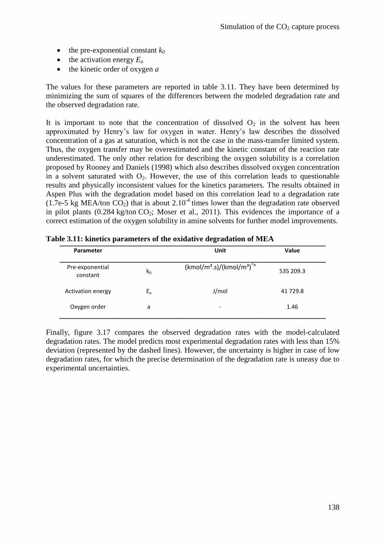
Simulation of the CO2 capture process

138

the pre-exponential constant k0

the activation energy Ea

the kinetic order of oxygen a

The values for these parameters are reported in table 3.11. They have been determined by

minimizing the sum of squares of the differences between the modeled degradation rate and

the observed degradation rate.

It is important to note that the concentration of dissolved O2 in the solvent has been

approximated by Henry’s law for oxygen in water. Henry’s law describes the dissolved

concentration of a gas at saturation, which is not the case in the mass-transfer limited system.

Thus, the oxygen transfer may be overestimated and the kinetic constant of the reaction rate

underestimated. The only other relation for describing the oxygen solubility is a correlation

proposed by Rooney and Daniels (1998) which also describes dissolved oxygen concentration

in a solvent saturated with O2. However, the use of this correlation leads to questionable

results and physically inconsistent values for the kinetics parameters. The results obtained in

Aspen Plus with the degradation model based on this correlation lead to a degradation rate

(1.7e-5 kg MEA/ton CO2) that is about 2.10-4

times lower than the degradation rate observed

in pilot plants (0.284 kg/ton CO2; Moser et al., 2011). This evidences the importance of a

correct estimation of the oxygen solubility in amine solvents for further model improvements.

Table 3.11: kinetics parameters of the oxidative degradation of MEA

Parameter Unit Value

Pre-exponential constant

k0 (kmol/m³.s)/(kmol/m³)^a

535 209.3

Activation energy Ea J/mol 41 729.8

Oxygen order a - 1.46

Finally, figure 3.17 compares the observed degradation rates with the model-calculated

degradation rates. The model predicts most experimental degradation rates with less than 15%

deviation (represented by the dashed lines). However, the uncertainty is higher in case of low

degradation rates, for which the precise determination of the degradation rate is uneasy due to

experimental uncertainties.

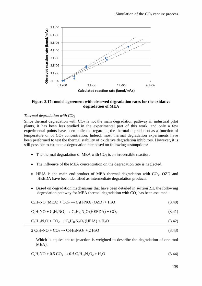
Simulation of the CO2 capture process

139

Figure 3.17: model agreement with observed degradation rates for the oxidative

degradation of MEA

Thermal degradation with CO2

Since thermal degradation with CO2 is not the main degradation pathway in industrial pilot

plants, it has been less studied in the experimental part of this work, and only a few

experimental points have been collected regarding the thermal degradation as a function of

temperature or of CO2 concentration. Indeed, most thermal degradation experiments have

been performed to test the thermal stability of oxidative degradation inhibitors. However, it is

still possible to estimate a degradation rate based on following assumptions:

The thermal degradation of MEA with CO2 is an irreversible reaction.

The influence of the MEA concentration on the degradation rate is neglected.

HEIA is the main end-product of MEA thermal degradation with CO2. OZD and

HEEDA have been identified as intermediate degradation products.

Based on degradation mechanisms that have been detailed in section 2.1, the following

degradation pathway for MEA thermal degradation with CO2 has been assumed:

C2H7NO (MEA) + CO2 → C3H5NO2 (OZD) + H2O (3.40)

C2H7NO + C3H5NO2 → C4H12N2O (HEEDA) + CO2 (3.41)

C4H12N2O + CO2 → C5H10N2O2 (HEIA) + H2O (3.42)

2 C2H7NO + CO2 → C5H10N2O2 + 2 H2O (3.43)

Which is equivalent to (reaction is weighted to describe the degradation of one mol

MEA):

C2H7NO + 0.5 CO2 → 0.5 C5H10N2O2 + H2O (3.44)

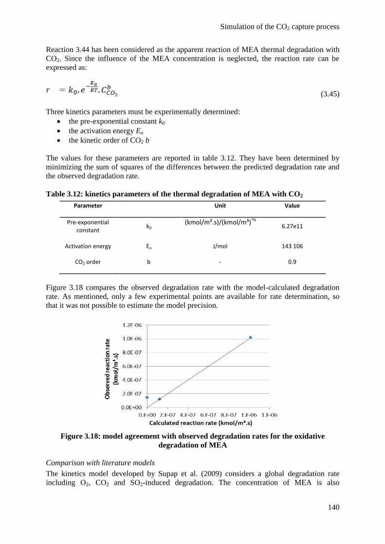
Simulation of the CO2 capture process

140

Reaction 3.44 has been considered as the apparent reaction of MEA thermal degradation with

CO2. Since the influence of the MEA concentration is neglected, the reaction rate can be

expressed as:

(3.45)

Three kinetics parameters must be experimentally determined:

the pre-exponential constant k0

the activation energy Ea

the kinetic order of CO2 b

The values for these parameters are reported in table 3.12. They have been determined by

minimizing the sum of squares of the differences between the predicted degradation rate and

the observed degradation rate.

Table 3.12: kinetics parameters of the thermal degradation of MEA with CO2

Parameter Unit Value

Pre-exponential constant

k0 (kmol/m³.s)/(kmol/m³)^b

6.27e11

Activation energy Ea J/mol 143 106

CO2 order b - 0.9

Figure 3.18 compares the observed degradation rate with the model-calculated degradation

rate. As mentioned, only a few experimental points are available for rate determination, so

that it was not possible to estimate the model precision.

Figure 3.18: model agreement with observed degradation rates for the oxidative

degradation of MEA

Comparison with literature models

The kinetics model developed by Supap et al. (2009) considers a global degradation rate

including O2, CO2 and SO2-induced degradation. The concentration of MEA is also

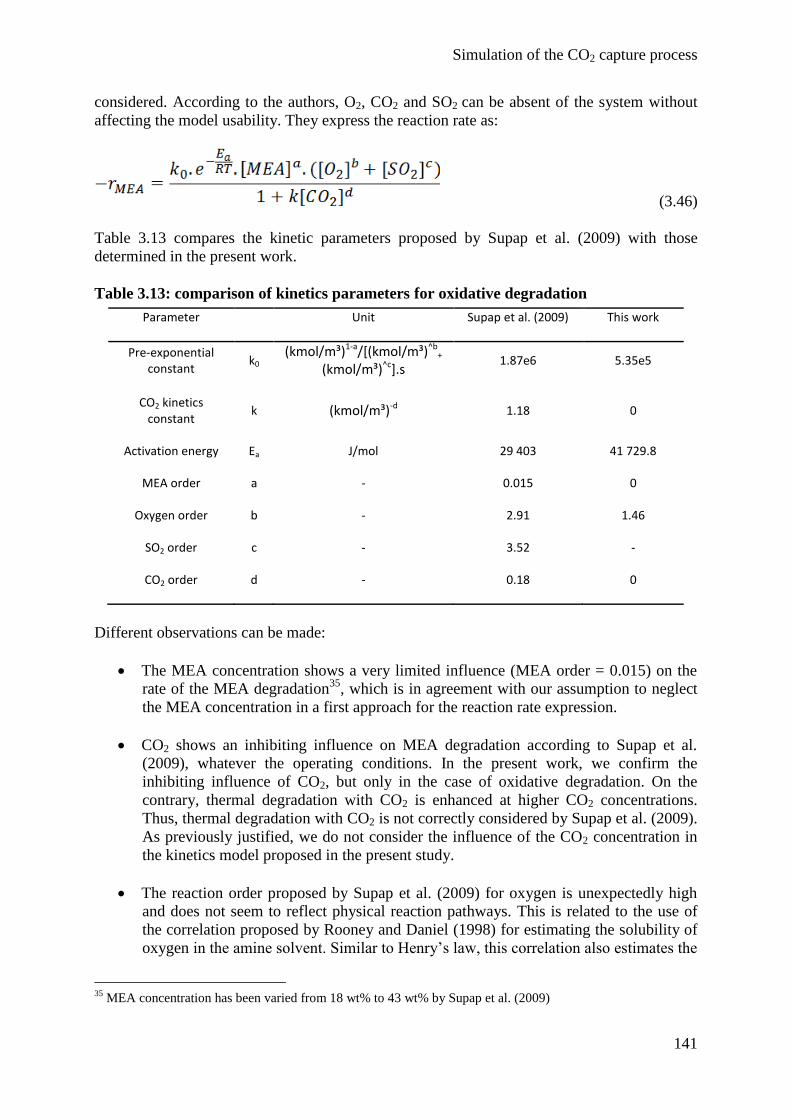
Simulation of the CO2 capture process

141

considered. According to the authors, O2, CO2 and SO2 can be absent of the system without

affecting the model usability. They express the reaction rate as:

(3.46)

Table 3.13 compares the kinetic parameters proposed by Supap et al. (2009) with those

determined in the present work.

Table 3.13: comparison of kinetics parameters for oxidative degradation

Parameter Unit Supap et al. (2009) This work

Pre-exponential constant

k0 (kmol/m³)1-a/[(kmol/m³)^b

+

(kmol/m³)^c].s 1.87e6 5.35e5

CO2 kinetics constant

k (kmol/m³)-d 1.18 0

Activation energy Ea J/mol 29 403 41 729.8

MEA order a - 0.015 0

Oxygen order b - 2.91 1.46

SO2 order c - 3.52 -

CO2 order d - 0.18 0

Different observations can be made:

The MEA concentration shows a very limited influence (MEA order = 0.015) on the

rate of the MEA degradation35

, which is in agreement with our assumption to neglect

the MEA concentration in a first approach for the reaction rate expression.

CO2 shows an inhibiting influence on MEA degradation according to Supap et al.

(2009), whatever the operating conditions. In the present work, we confirm the

inhibiting influence of CO2, but only in the case of oxidative degradation. On the

contrary, thermal degradation with CO2 is enhanced at higher CO2 concentrations.

Thus, thermal degradation with CO2 is not correctly considered by Supap et al. (2009).

As previously justified, we do not consider the influence of the CO2 concentration in

the kinetics model proposed in the present study.

The reaction order proposed by Supap et al. (2009) for oxygen is unexpectedly high

and does not seem to reflect physical reaction pathways. This is related to the use of

the correlation proposed by Rooney and Daniel (1998) for estimating the solubility of

oxygen in the amine solvent. Similar to Henry’s law, this correlation also estimates the

35

MEA concentration has been varied from 18 wt% to 43 wt% by Supap et al. (2009)

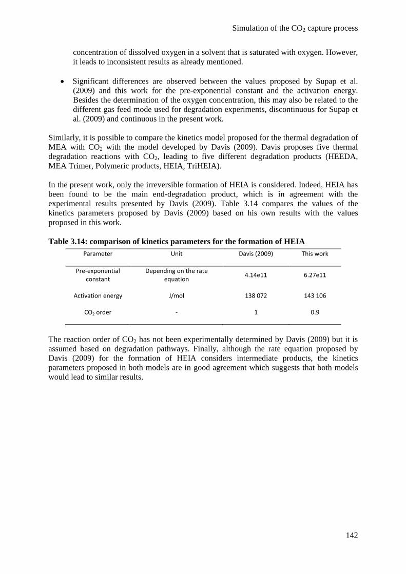
Simulation of the CO2 capture process

142

concentration of dissolved oxygen in a solvent that is saturated with oxygen. However,

it leads to inconsistent results as already mentioned.

Significant differences are observed between the values proposed by Supap et al.

(2009) and this work for the pre-exponential constant and the activation energy.

Besides the determination of the oxygen concentration, this may also be related to the

different gas feed mode used for degradation experiments, discontinuous for Supap et

al. (2009) and continuous in the present work.

Similarly, it is possible to compare the kinetics model proposed for the thermal degradation of

MEA with CO2 with the model developed by Davis (2009). Davis proposes five thermal

degradation reactions with CO2, leading to five different degradation products (HEEDA,

MEA Trimer, Polymeric products, HEIA, TriHEIA).

In the present work, only the irreversible formation of HEIA is considered. Indeed, HEIA has

been found to be the main end-degradation product, which is in agreement with the

experimental results presented by Davis (2009). Table 3.14 compares the values of the

kinetics parameters proposed by Davis (2009) based on his own results with the values

proposed in this work.

Table 3.14: comparison of kinetics parameters for the formation of HEIA

Parameter Unit Davis (2009) This work

Pre-exponential constant

Depending on the rate equation

4.14e11 6.27e11

Activation energy J/mol 138 072 143 106

CO2 order - 1 0.9

The reaction order of CO2 has not been experimentally determined by Davis (2009) but it is

assumed based on degradation pathways. Finally, although the rate equation proposed by

Davis (2009) for the formation of HEIA considers intermediate products, the kinetics

parameters proposed in both models are in good agreement which suggests that both models

would lead to similar results.

Simulation of the CO2 capture process

143

4. Simulation results

Most CO2 capture models have been developed to study the influence of operating variables

on the process energy requirement. However, the process environmental penalty has not been

considered but in very few studies. For instance, oxidative degradation has been integrated in

only one process modeling study (Thong et al., 2012), which relies on questionable

assumptions regarding experimental data. Thus, the present section explores different

modeling pathways and finally proposes a model that considers both the energy and the

environmental penalty of the CO2 capture process.

First, the models based on design data of the Mobile Pilot Unit are compared to evaluate the

influence of the equilibrium and rate-based approaches for modeling the CO2 reactive

absorption. The influence of operating parameters on the process energy requirement is

studied for both models, and the column temperature profiles are compared.

Then, the potential of unsteady-state simulations is evidenced by a practical application using

the dynamic model. It is supposed that the energy available for the capture plant is reduced

due to increased electricity demand during daily peak hours. Two different strategies for

temporarily reducing the CO2 capture rate, and thus the energy requirement of the capture

plant, are evaluated.

Finally, results gained with the steady-state, rate-based degradation model are presented. The

influence of the main operating variables on solvent degradation and on emission of

degradation products is reported. Furthermore, alternative flowsheet configurations are

evaluated from an environmental point of view as well. Finally, optimal operating conditions

are proposed that consider the process energy requirement as well as the emission of

degradation products.

4.1 Equilibrium and rate-based model comparison

Two different models have been developed based on design data of a Mobile Pilot Unit as

described in section 3.1. The equilibrium model makes the assumption that mass transfer

columns can be modeled by the succession of equilibrium stages in which mass and heat

transfer limitations are neglected. On the contrary, the rate-based model rigorously calculates

the mass transfer in the columns. Moreover, the rate-based model also considers the chemical

kinetics limitations of the CO2 reactive absorption. In this section, a sensitivity analysis of key

operating variables is performed using both models. Then, the temperature profiles of the

mass transfer columns are discussed for each model.

Sensitivity analysis

Three main process variables have been identified based on the works of Freguia and

Rochelle (2003) and Abu-Zahra (2007a). These variables are the solvent flow rate, the

pressure of the stripper and the concentration of the MEA solution. A sensitivity analysis is

performed by varying successively each variable while other operating parameters are kept

constant. The flue gas flow rate equals 2500 Nm³/h (14% CO2, 12% H2O, 6% O2, 68% N2)

and the CO2 capture rate is kept constant at 90%. However, no experimental data are available

for the simulated pilot plant. As a consequence, predicted behaviors are compared with values

reported in the literature when available, but no precise validation has been performed.

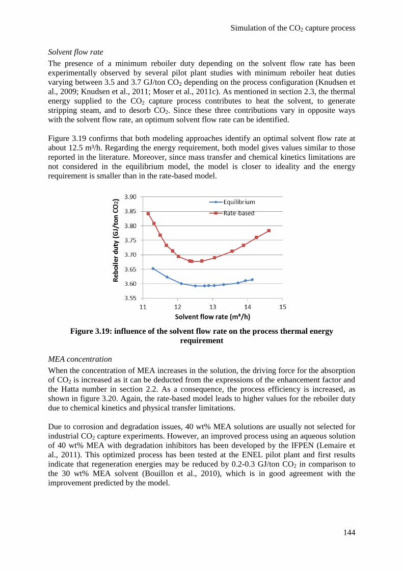
Simulation of the CO2 capture process

144

Solvent flow rate

The presence of a minimum reboiler duty depending on the solvent flow rate has been

experimentally observed by several pilot plant studies with minimum reboiler heat duties

varying between 3.5 and 3.7 GJ/ton CO2 depending on the process configuration (Knudsen et

al., 2009; Knudsen et al., 2011; Moser et al., 2011c). As mentioned in section 2.3, the thermal

energy supplied to the CO2 capture process contributes to heat the solvent, to generate

stripping steam, and to desorb CO2. Since these three contributions vary in opposite ways

with the solvent flow rate, an optimum solvent flow rate can be identified.

Figure 3.19 confirms that both modeling approaches identify an optimal solvent flow rate at

about 12.5 m³/h. Regarding the energy requirement, both model gives values similar to those

reported in the literature. Moreover, since mass transfer and chemical kinetics limitations are

not considered in the equilibrium model, the model is closer to ideality and the energy

requirement is smaller than in the rate-based model.

Figure 3.19: influence of the solvent flow rate on the process thermal energy

requirement

MEA concentration

When the concentration of MEA increases in the solution, the driving force for the absorption

of CO2 is increased as it can be deducted from the expressions of the enhancement factor and

the Hatta number in section 2.2. As a consequence, the process efficiency is increased, as

shown in figure 3.20. Again, the rate-based model leads to higher values for the reboiler duty

due to chemical kinetics and physical transfer limitations.

Due to corrosion and degradation issues, 40 wt% MEA solutions are usually not selected for

industrial CO2 capture experiments. However, an improved process using an aqueous solution

of 40 wt% MEA with degradation inhibitors has been developed by the IFPEN (Lemaire et

al., 2011). This optimized process has been tested at the ENEL pilot plant and first results

indicate that regeneration energies may be reduced by 0.2-0.3 GJ/ton CO2 in comparison to

the 30 wt% MEA solvent (Bouillon et al., 2010), which is in good agreement with the

improvement predicted by the model.

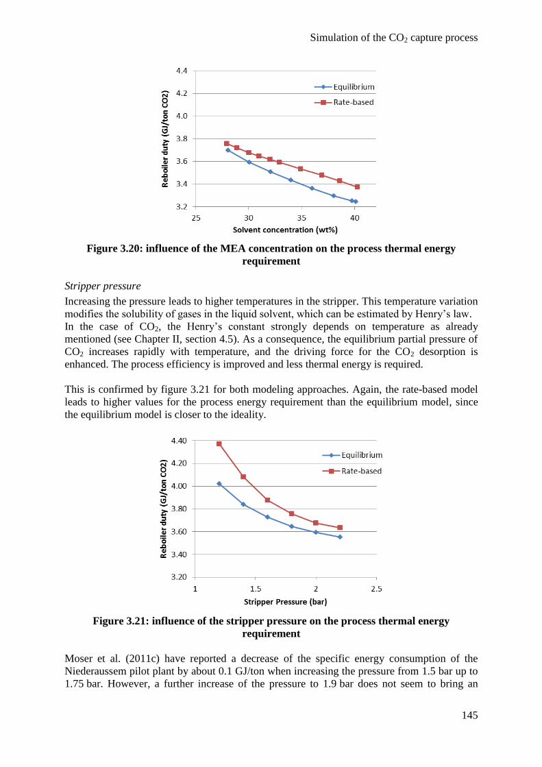
Simulation of the CO2 capture process

145

Figure 3.20: influence of the MEA concentration on the process thermal energy

requirement

Stripper pressure

Increasing the pressure leads to higher temperatures in the stripper. This temperature variation

modifies the solubility of gases in the liquid solvent, which can be estimated by Henry’s law.

In the case of CO2, the Henry’s constant strongly depends on temperature as already

mentioned (see Chapter II, section 4.5). As a consequence, the equilibrium partial pressure of

CO2 increases rapidly with temperature, and the driving force for the CO2 desorption is

enhanced. The process efficiency is improved and less thermal energy is required.

This is confirmed by figure 3.21 for both modeling approaches. Again, the rate-based model

leads to higher values for the process energy requirement than the equilibrium model, since

the equilibrium model is closer to the ideality.

Figure 3.21: influence of the stripper pressure on the process thermal energy

requirement

Moser et al. (2011c) have reported a decrease of the specific energy consumption of the

Niederaussem pilot plant by about 0.1 GJ/ton when increasing the pressure from 1.5 bar up to

1.75 bar. However, a further increase of the pressure to 1.9 bar does not seem to bring an

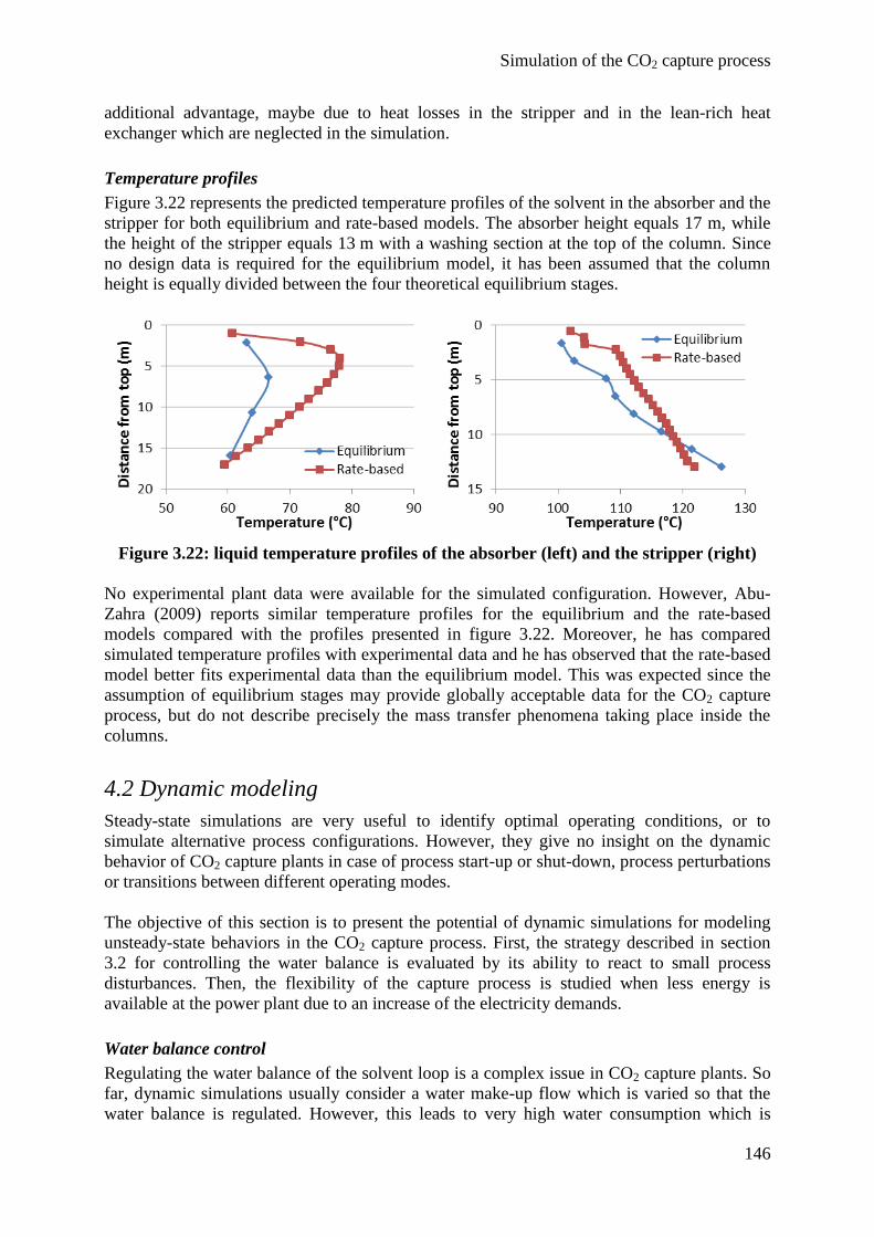
Simulation of the CO2 capture process

146

additional advantage, maybe due to heat losses in the stripper and in the lean-rich heat

exchanger which are neglected in the simulation.

Temperature profiles

Figure 3.22 represents the predicted temperature profiles of the solvent in the absorber and the

stripper for both equilibrium and rate-based models. The absorber height equals 17 m, while

the height of the stripper equals 13 m with a washing section at the top of the column. Since

no design data is required for the equilibrium model, it has been assumed that the column

height is equally divided between the four theoretical equilibrium stages.

Figure 3.22: liquid temperature profiles of the absorber (left) and the stripper (right)

No experimental plant data were available for the simulated configuration. However, Abu-

Zahra (2009) reports similar temperature profiles for the equilibrium and the rate-based

models compared with the profiles presented in figure 3.22. Moreover, he has compared

simulated temperature profiles with experimental data and he has observed that the rate-based

model better fits experimental data than the equilibrium model. This was expected since the

assumption of equilibrium stages may provide globally acceptable data for the CO2 capture

process, but do not describe precisely the mass transfer phenomena taking place inside the

columns.

4.2 Dynamic modeling

Steady-state simulations are very useful to identify optimal operating conditions, or to

simulate alternative process configurations. However, they give no insight on the dynamic

behavior of CO2 capture plants in case of process start-up or shut-down, process perturbations

or transitions between different operating modes.

The objective of this section is to present the potential of dynamic simulations for modeling

unsteady-state behaviors in the CO2 capture process. First, the strategy described in section

3.2 for controlling the water balance is evaluated by its ability to react to small process

disturbances. Then, the flexibility of the capture process is studied when less energy is

available at the power plant due to an increase of the electricity demands.

Water balance control

Regulating the water balance of the solvent loop is a complex issue in CO2 capture plants. So

far, dynamic simulations usually consider a water make-up flow which is varied so that the

water balance is regulated. However, this leads to very high water consumption which is

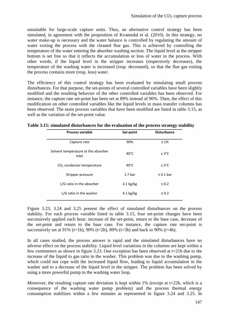
Simulation of the CO2 capture process

147

unsuitable for large-scale capture units. Thus, an alternative control strategy has been

simulated, in agreement with the proposition of Kvamsdal et al. (2010). In this strategy, no

water make-up is necessary and the water balance is controlled by regulating the amount of

water exiting the process with the cleaned flue gas. This is achieved by controlling the

temperature of the water entering the absorber washing section. The liquid level at the stripper

bottom is set free so that it reflects the accumulation or loss of water in the process. With

other words, if the liquid level in the stripper increases (respectively decreases), the

temperature of the washing water is increased (resp. decreased), so that the flue gas exiting

the process contains more (resp. less) water.

The efficiency of this control strategy has been evaluated by simulating small process

disturbances. For that purpose, the set-points of several controlled variables have been slightly

modified and the resulting behavior of the other controlled variables has been observed. For

instance, the capture rate set-point has been set at 89% instead of 90%. Then, the effect of this

modification on other controlled variables like the liquid levels in mass transfer columns has

been observed. The main process variables that have been modified are listed in table 3.15, as

well as the variation of the set-point value.

Table 3.15: simulated disturbances for the evaluation of the process strategy stability

Process variable Set-point Disturbance

Capture rate 90% ± 1%

Solvent temperature at the absorber inlet

40°C ± 3°C

CO2 condenser temperature 40°C ± 3°C

Stripper pressure 1.7 bar ± 0.1 bar

L/G ratio in the absorber 4.1 kg/kg ± 0.2

L/G ratio in the washer 4.1 kg/kg ± 0.2

Figure 3.23, 3.24 and 3.25 present the effect of simulated disturbances on the process

stability. For each process variable listed in table 3.15, four set-point changes have been

successively applied each hour: increase of the set-point, return to the base case, decrease of

the set-point and return to the base case. For instance, the capture rate set-point is

successively set at 91% (t=1h), 90% (t=2h), 89% (t=3h) and back to 90% (t=4h).

In all cases studied, the process answer is rapid and the simulated disturbances have no

adverse effect on the process stability. Liquid level variations in the columns are kept within a

few centimeters as shown in figure 3.23. One exception has been observed at t=21h due to the

increase of the liquid to gas ratio in the washer. This problem was due to the washing pump,

which could not cope with the increased liquid flow, leading to liquid accumulation in the

washer and to a decrease of the liquid level in the stripper. The problem has been solved by

using a more powerful pump in the washing water loop.

Moreover, the resulting capture rate deviation is kept within 1% (except at t=22h, which is a

consequence of the washing water pump problem) and the process thermal energy

consumption stabilizes within a few minutes as represented in figure 3.24 and 3.25. In

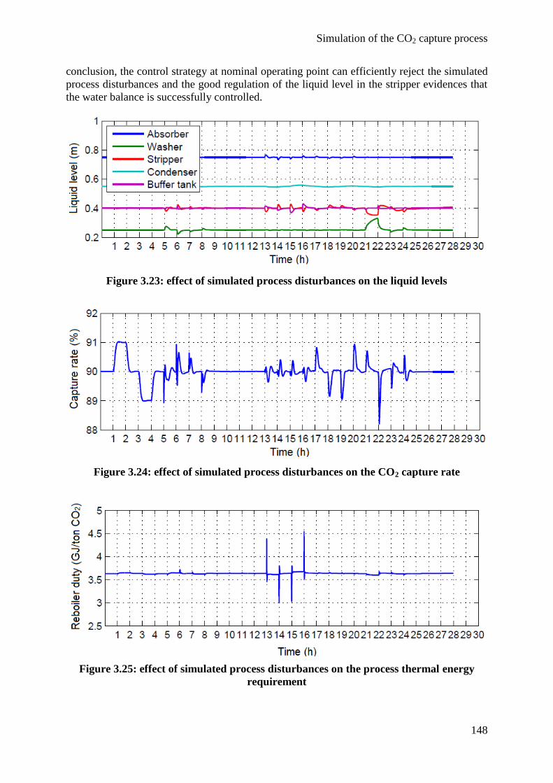
Simulation of the CO2 capture process

148

conclusion, the control strategy at nominal operating point can efficiently reject the simulated

process disturbances and the good regulation of the liquid level in the stripper evidences that

the water balance is successfully controlled.

Figure 3.23: effect of simulated process disturbances on the liquid levels

Figure 3.24: effect of simulated process disturbances on the CO2 capture rate

Figure 3.25: effect of simulated process disturbances on the process thermal energy

requirement

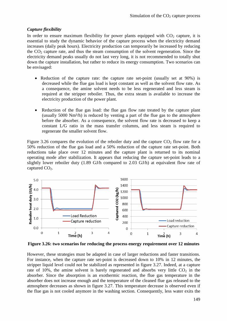
Simulation of the CO2 capture process

149

Capture flexibility

In order to ensure maximum flexibility for power plants equipped with CO2 capture, it is

essential to study the dynamic behavior of the capture process when the electricity demand

increases (daily peak hours). Electricity production can temporarily be increased by reducing

the CO2 capture rate, and thus the steam consumption of the solvent regeneration. Since the

electricity demand peaks usually do not last very long, it is not recommended to totally shut

down the capture installation, but rather to reduce its energy consumption. Two scenarios can

be envisaged:

Reduction of the capture rate: the capture rate set-point (usually set at 90%) is

decreased while the flue gas load is kept constant as well as the solvent flow rate. As

a consequence, the amine solvent needs to be less regenerated and less steam is

required at the stripper reboiler. Thus, the extra steam is available to increase the

electricity production of the power plant.

Reduction of the flue gas load: the flue gas flow rate treated by the capture plant

(usually 5000 Nm³/h) is reduced by venting a part of the flue gas to the atmosphere

before the absorber. As a consequence, the solvent flow rate is decreased to keep a

constant L/G ratio in the mass transfer columns, and less steam is required to

regenerate the smaller solvent flow.

Figure 3.26 compares the evolution of the reboiler duty and the capture CO2 flow rate for a

50% reduction of the flue gas load and a 50% reduction of the capture rate set-point. Both

reductions take place over 12 minutes and the capture plant is returned to its nominal

operating mode after stabilization. It appears that reducing the capture set-point leads to a

slightly lower reboiler duty (1.89 GJ/h compared to 2.03 GJ/h) at equivalent flow rate of

captured CO2.

Figure 3.26: two scenarios for reducing the process energy requirement over 12 minutes

However, these strategies must be adapted in case of larger reductions and faster transitions.

For instance, when the capture rate set-point is decreased down to 10% in 12 minutes, the

stripper liquid level could not be stabilized as represented in figure 3.27. Indeed, at a capture

rate of 10%, the amine solvent is barely regenerated and absorbs very little CO2 in the

absorber. Since the absorption is an exothermic reaction, the flue gas temperature in the

absorber does not increase enough and the temperature of the cleaned flue gas released to the

atmosphere decreases as shown in figure 3.27. This temperature decrease is observed even if

the flue gas is not cooled anymore in the washing section. Consequently, less water exits the

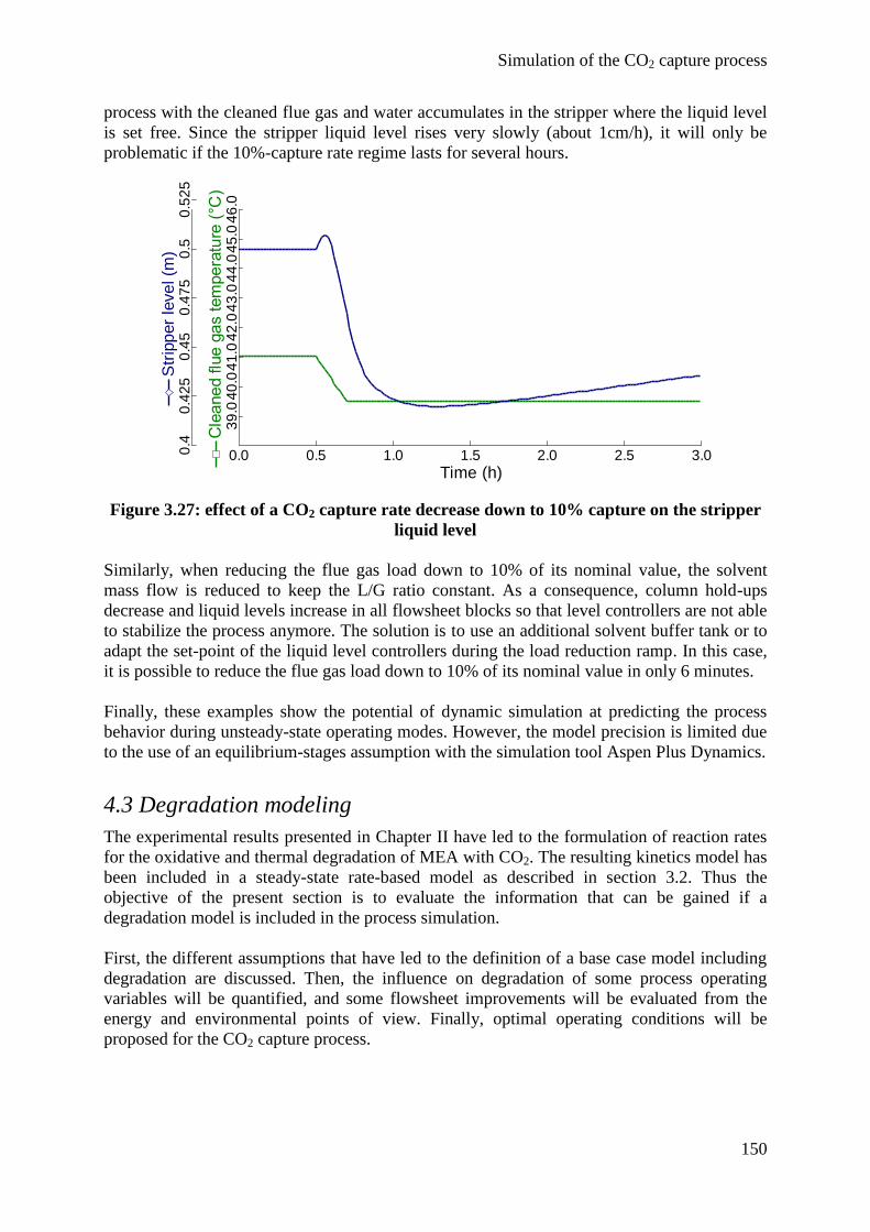
Simulation of the CO2 capture process

150

process with the cleaned flue gas and water accumulates in the stripper where the liquid level

is set free. Since the stripper liquid level rises very slowly (about 1cm/h), it will only be

problematic if the 10%-capture rate regime lasts for several hours.

Time (h)

Str

ipp

er

leve

l (m

)

Cle

ane

d f

lue

ga

s t

em

pe

ratu

re (

°C)

Str

ipp

er

leve

l (m

)

0.0 0.5 1.0 1.5 2.0 2.5 3.0

39

.04

0.0

41

.04

2.0

43

.04

4.0

45

.04

6.0

0.4

0.4

25

0.4

50

.47

50

.50

.52

5

Figure 3.27: effect of a CO2 capture rate decrease down to 10% capture on the stripper

liquid level

Similarly, when reducing the flue gas load down to 10% of its nominal value, the solvent

mass flow is reduced to keep the L/G ratio constant. As a consequence, column hold-ups

decrease and liquid levels increase in all flowsheet blocks so that level controllers are not able

to stabilize the process anymore. The solution is to use an additional solvent buffer tank or to

adapt the set-point of the liquid level controllers during the load reduction ramp. In this case,

it is possible to reduce the flue gas load down to 10% of its nominal value in only 6 minutes.

Finally, these examples show the potential of dynamic simulation at predicting the process

behavior during unsteady-state operating modes. However, the model precision is limited due

to the use of an equilibrium-stages assumption with the simulation tool Aspen Plus Dynamics.

4.3 Degradation modeling

The experimental results presented in Chapter II have led to the formulation of reaction rates

for the oxidative and thermal degradation of MEA with CO2. The resulting kinetics model has

been included in a steady-state rate-based model as described in section 3.2. Thus the

objective of the present section is to evaluate the information that can be gained if a

degradation model is included in the process simulation.

First, the different assumptions that have led to the definition of a base case model including

degradation are discussed. Then, the influence on degradation of some process operating

variables will be quantified, and some flowsheet improvements will be evaluated from the

energy and environmental points of view. Finally, optimal operating conditions will be

proposed for the CO2 capture process.

Simulation of the CO2 capture process

151

Base case degradation

In this section, three main assumptions regarding the modeling of degradation reactions are

first justified: the use of a steady-state model, the consideration of degradation reactions in the

mass transfer columns, and the absence of solvent purge and make-up. These assumptions

have led to the definition of a base case model of the CO2 capture process with assessment of

solvent degradation. Finally, the degradation extent observed in the base case is discussed.

Steady-state assumption

As already mentioned, degradation reactions show a slow kinetics so that it is difficult to

observe the formation of degradation products over a short time range. Thus, one could think

that the best way to include degradation in a process simulation is to run a dynamic simulation

of the process with degradation reactions and to observe the accumulation of degradation

products over large time ranges. However, dynamic simulations are not adapted to describe

small modifications over long time scale (several months). Moreover, it is essential to

consider mass transfer limitations when modeling degradation phenomena, and the developed

model using Aspen Plus Dynamics only allows the use of equilibrium models. Finally, it has

been decided to include the degradation in a steady-state model.

Degradation in mass transfer columns

Thong et al. (2012) have proposed to model degradation reactions taking place in the capture

process in a separate reactor that would be fed with solvent and for which the solvent

residence time can be arbitrarily varied from a few seconds to several months. This approach

has not been selected for three main reasons:

This approach implies to decouple the time scale of the degradation reactions from the

CO2 capture process, making it unsuited to study the influence of operating process

parameters on degradation.

It appears from the experimental study that it is necessary to consider mass transfer

limitations while modeling solvent degradation, which is not the case in the reactor

model proposed by Thong et al. (2012).

There is no gas supply in the separate reactors proposed by Thong et al. (2012), so that

the available oxygen is rapidly consumed and the degradation extent is severely

underestimated, whatever the residence time in the degradation reactor.

Thus it has been assumed that the best way to model degradation reactions is to include them

in the absorber and stripper columns, which better reflects the actual process operating

conditions. Degradation in the other flowsheet blocks has been neglected in a first approach.

Solvent purge and make-up

The degradation model has been initially designed with a purge and a MEA make-up stream

as represented in figure 3.28.

The optimal purge flow rate can be determined based on following assumptions:

Oxidative degradation products are formed in higher quantities than thermal

degradation products.

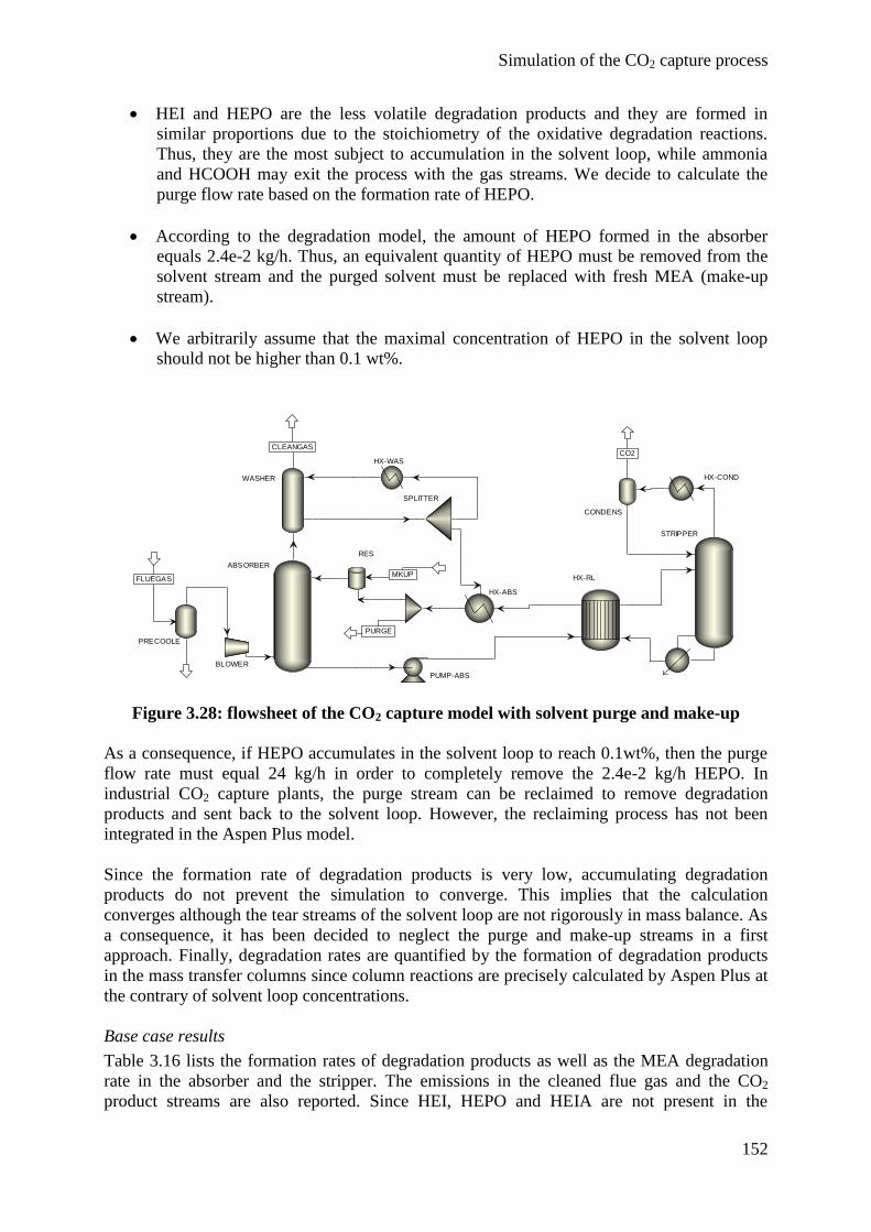
Simulation of the CO2 capture process

152

HEI and HEPO are the less volatile degradation products and they are formed in

similar proportions due to the stoichiometry of the oxidative degradation reactions.

Thus, they are the most subject to accumulation in the solvent loop, while ammonia

and HCOOH may exit the process with the gas streams. We decide to calculate the

purge flow rate based on the formation rate of HEPO.

According to the degradation model, the amount of HEPO formed in the absorber

equals 2.4e-2 kg/h. Thus, an equivalent quantity of HEPO must be removed from the

solvent stream and the purged solvent must be replaced with fresh MEA (make-up

stream).

We arbitrarily assume that the maximal concentration of HEPO in the solvent loop

should not be higher than 0.1 wt%.

ABSORBER

PUMP-ABS

WASHER

STRIPPER

CONDENS

HX-RL

SPLITTER

BLOWER

PRECOOLE

HX-WAS

HX-COND

HX-ABS

RES

CLEANGAS

CO2

FLUEGAS

PURGE

MKUP

Figure 3.28: flowsheet of the CO2 capture model with solvent purge and make-up

As a consequence, if HEPO accumulates in the solvent loop to reach 0.1wt%, then the purge

flow rate must equal 24 kg/h in order to completely remove the 2.4e-2 kg/h HEPO. In

industrial CO2 capture plants, the purge stream can be reclaimed to remove degradation

products and sent back to the solvent loop. However, the reclaiming process has not been

integrated in the Aspen Plus model.

Since the formation rate of degradation products is very low, accumulating degradation

products do not prevent the simulation to converge. This implies that the calculation

converges although the tear streams of the solvent loop are not rigorously in mass balance. As

a consequence, it has been decided to neglect the purge and make-up streams in a first

approach. Finally, degradation rates are quantified by the formation of degradation products

in the mass transfer columns since column reactions are precisely calculated by Aspen Plus at

the contrary of solvent loop concentrations.

Base case results

Table 3.16 lists the formation rates of degradation products as well as the MEA degradation

rate in the absorber and the stripper. The emissions in the cleaned flue gas and the CO2

product streams are also reported. Since HEI, HEPO and HEIA are not present in the

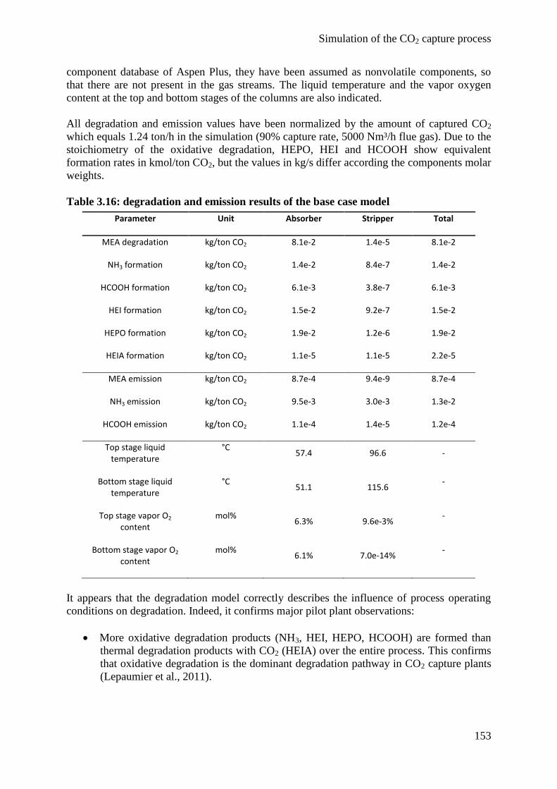
Simulation of the CO2 capture process

153

component database of Aspen Plus, they have been assumed as nonvolatile components, so

that there are not present in the gas streams. The liquid temperature and the vapor oxygen

content at the top and bottom stages of the columns are also indicated.

All degradation and emission values have been normalized by the amount of captured CO2

which equals 1.24 ton/h in the simulation (90% capture rate, 5000 Nm³/h flue gas). Due to the

stoichiometry of the oxidative degradation, HEPO, HEI and HCOOH show equivalent

formation rates in kmol/ton CO2, but the values in kg/s differ according the components molar

weights.

Table 3.16: degradation and emission results of the base case model

Parameter Unit Absorber Stripper Total

MEA degradation kg/ton CO2 8.1e-2 1.4e-5 8.1e-2

NH3 formation kg/ton CO2 1.4e-2 8.4e-7 1.4e-2

HCOOH formation kg/ton CO2 6.1e-3 3.8e-7 6.1e-3

HEI formation kg/ton CO2 1.5e-2 9.2e-7 1.5e-2

HEPO formation kg/ton CO2 1.9e-2 1.2e-6 1.9e-2

HEIA formation kg/ton CO2 1.1e-5 1.1e-5 2.2e-5

MEA emission kg/ton CO2 8.7e-4 9.4e-9 8.7e-4

NH3 emission kg/ton CO2 9.5e-3 3.0e-3 1.3e-2

HCOOH emission kg/ton CO2 1.1e-4 1.4e-5 1.2e-4

Top stage liquid temperature

°C 57.4 96.6 -

Bottom stage liquid temperature

°C 51.1 115.6

-

Top stage vapor O2 content

mol% 6.3% 9.6e-3%

-

Bottom stage vapor O2 content

mol% 6.1% 7.0e-14%

-

It appears that the degradation model correctly describes the influence of process operating

conditions on degradation. Indeed, it confirms major pilot plant observations:

More oxidative degradation products (NH3, HEI, HEPO, HCOOH) are formed than

thermal degradation products with CO2 (HEIA) over the entire process. This confirms

that oxidative degradation is the dominant degradation pathway in CO2 capture plants

(Lepaumier et al., 2011).

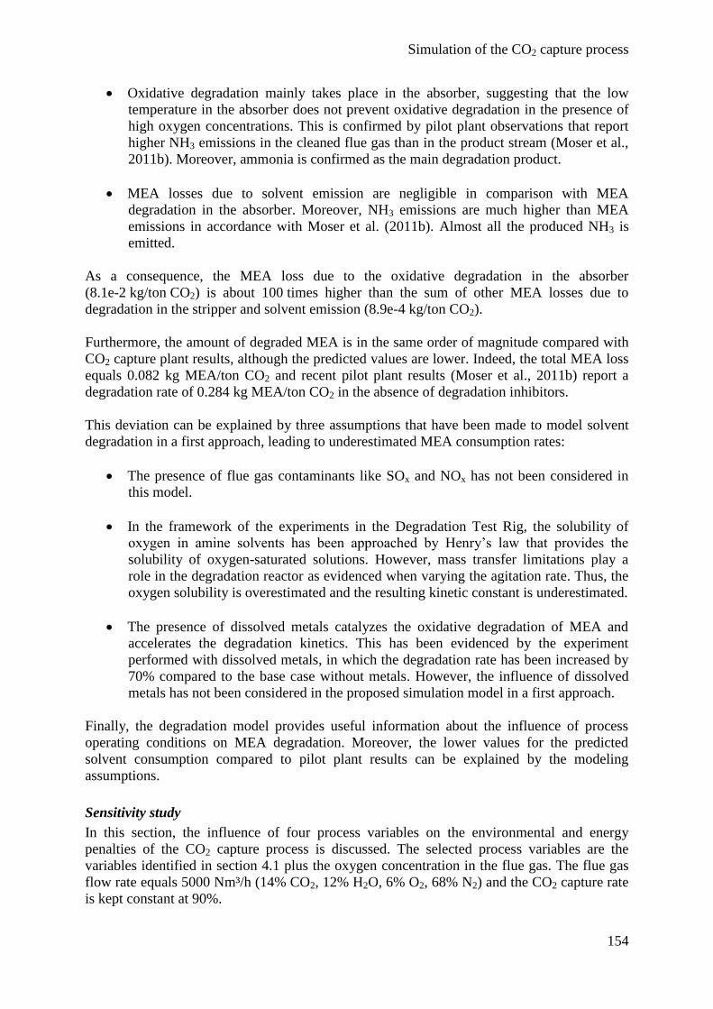
Simulation of the CO2 capture process

154

Oxidative degradation mainly takes place in the absorber, suggesting that the low

temperature in the absorber does not prevent oxidative degradation in the presence of

high oxygen concentrations. This is confirmed by pilot plant observations that report

higher NH3 emissions in the cleaned flue gas than in the product stream (Moser et al.,

2011b). Moreover, ammonia is confirmed as the main degradation product.

MEA losses due to solvent emission are negligible in comparison with MEA

degradation in the absorber. Moreover, NH3 emissions are much higher than MEA

emissions in accordance with Moser et al. (2011b). Almost all the produced NH3 is

emitted.

As a consequence, the MEA loss due to the oxidative degradation in the absorber

(8.1e-2 kg/ton CO2) is about 100 times higher than the sum of other MEA losses due to

degradation in the stripper and solvent emission (8.9e-4 kg/ton CO2).

Furthermore, the amount of degraded MEA is in the same order of magnitude compared with

CO2 capture plant results, although the predicted values are lower. Indeed, the total MEA loss

equals 0.082 kg MEA/ton CO2 and recent pilot plant results (Moser et al., 2011b) report a

degradation rate of 0.284 kg MEA/ton CO2 in the absence of degradation inhibitors.

This deviation can be explained by three assumptions that have been made to model solvent

degradation in a first approach, leading to underestimated MEA consumption rates:

The presence of flue gas contaminants like SOx and NOx has not been considered in

this model.

In the framework of the experiments in the Degradation Test Rig, the solubility of

oxygen in amine solvents has been approached by Henry’s law that provides the

solubility of oxygen-saturated solutions. However, mass transfer limitations play a

role in the degradation reactor as evidenced when varying the agitation rate. Thus, the

oxygen solubility is overestimated and the resulting kinetic constant is underestimated.

The presence of dissolved metals catalyzes the oxidative degradation of MEA and

accelerates the degradation kinetics. This has been evidenced by the experiment

performed with dissolved metals, in which the degradation rate has been increased by

70% compared to the base case without metals. However, the influence of dissolved

metals has not been considered in the proposed simulation model in a first approach.

Finally, the degradation model provides useful information about the influence of process

operating conditions on MEA degradation. Moreover, the lower values for the predicted

solvent consumption compared to pilot plant results can be explained by the modeling

assumptions.

Sensitivity study

In this section, the influence of four process variables on the environmental and energy

penalties of the CO2 capture process is discussed. The selected process variables are the

variables identified in section 4.1 plus the oxygen concentration in the flue gas. The flue gas

flow rate equals 5000 Nm³/h (14% CO2, 12% H2O, 6% O2, 68% N2) and the CO2 capture rate

is kept constant at 90%.

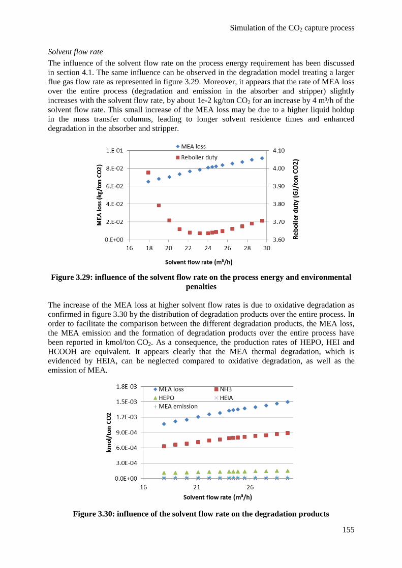
Simulation of the CO2 capture process

155

Solvent flow rate

The influence of the solvent flow rate on the process energy requirement has been discussed

in section 4.1. The same influence can be observed in the degradation model treating a larger

flue gas flow rate as represented in figure 3.29. Moreover, it appears that the rate of MEA loss

over the entire process (degradation and emission in the absorber and stripper) slightly

increases with the solvent flow rate, by about 1e-2 kg/ton CO2 for an increase by 4 m³/h of the

solvent flow rate. This small increase of the MEA loss may be due to a higher liquid holdup

in the mass transfer columns, leading to longer solvent residence times and enhanced

degradation in the absorber and stripper.

Figure 3.29: influence of the solvent flow rate on the process energy and environmental

penalties

The increase of the MEA loss at higher solvent flow rates is due to oxidative degradation as

confirmed in figure 3.30 by the distribution of degradation products over the entire process. In

order to facilitate the comparison between the different degradation products, the MEA loss,

the MEA emission and the formation of degradation products over the entire process have

been reported in kmol/ton CO2. As a consequence, the production rates of HEPO, HEI and

HCOOH are equivalent. It appears clearly that the MEA thermal degradation, which is

evidenced by HEIA, can be neglected compared to oxidative degradation, as well as the

emission of MEA.

Figure 3.30: influence of the solvent flow rate on the degradation products

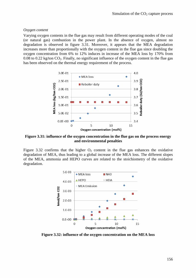
Simulation of the CO2 capture process

156

Oxygen content

Varying oxygen contents in the flue gas may result from different operating modes of the coal

(or natural gas) combustion in the power plant. In the absence of oxygen, almost no

degradation is observed in figure 3.31. Moreover, it appears that the MEA degradation

increases more than proportionally with the oxygen content in the flue gas since doubling the

oxygen concentration from 6% to 12% induces in increase of the MEA loss by 170% from

0.08 to 0.22 kg/ton CO2. Finally, no significant influence of the oxygen content in the flue gas

has been observed on the thermal energy requirement of the process.

Figure 3.31: influence of the oxygen concentration in the flue gas on the process energy

and environmental penalties

Figure 3.32 confirms that the higher O2 content in the flue gas enhances the oxidative

degradation of MEA, thus leading to a global increase of the MEA loss. The different slopes

of the MEA, ammonia and HEPO curves are related to the stoichiometry of the oxidative

degradation.

Figure 3.32: influence of the oxygen concentration on the MEA loss

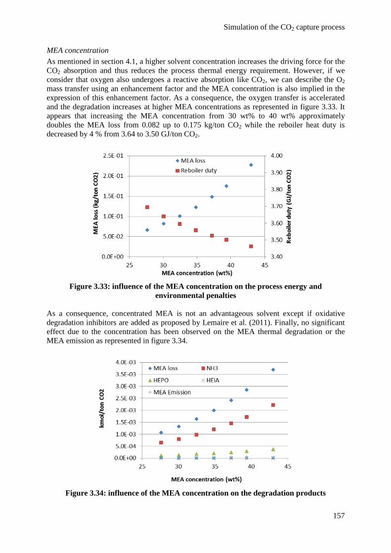
Simulation of the CO2 capture process

157

MEA concentration

As mentioned in section 4.1, a higher solvent concentration increases the driving force for the

CO2 absorption and thus reduces the process thermal energy requirement. However, if we

consider that oxygen also undergoes a reactive absorption like CO2, we can describe the O2

mass transfer using an enhancement factor and the MEA concentration is also implied in the

expression of this enhancement factor. As a consequence, the oxygen transfer is accelerated

and the degradation increases at higher MEA concentrations as represented in figure 3.33. It

appears that increasing the MEA concentration from 30 wt% to 40 wt% approximately

doubles the MEA loss from 0.082 up to 0.175 kg/ton CO2 while the reboiler heat duty is

decreased by 4 % from 3.64 to 3.50 GJ/ton CO2.

Figure 3.33: influence of the MEA concentration on the process energy and

environmental penalties

As a consequence, concentrated MEA is not an advantageous solvent except if oxidative

degradation inhibitors are added as proposed by Lemaire et al. (2011). Finally, no significant

effect due to the concentration has been observed on the MEA thermal degradation or the

MEA emission as represented in figure 3.34.

Figure 3.34: influence of the MEA concentration on the degradation products

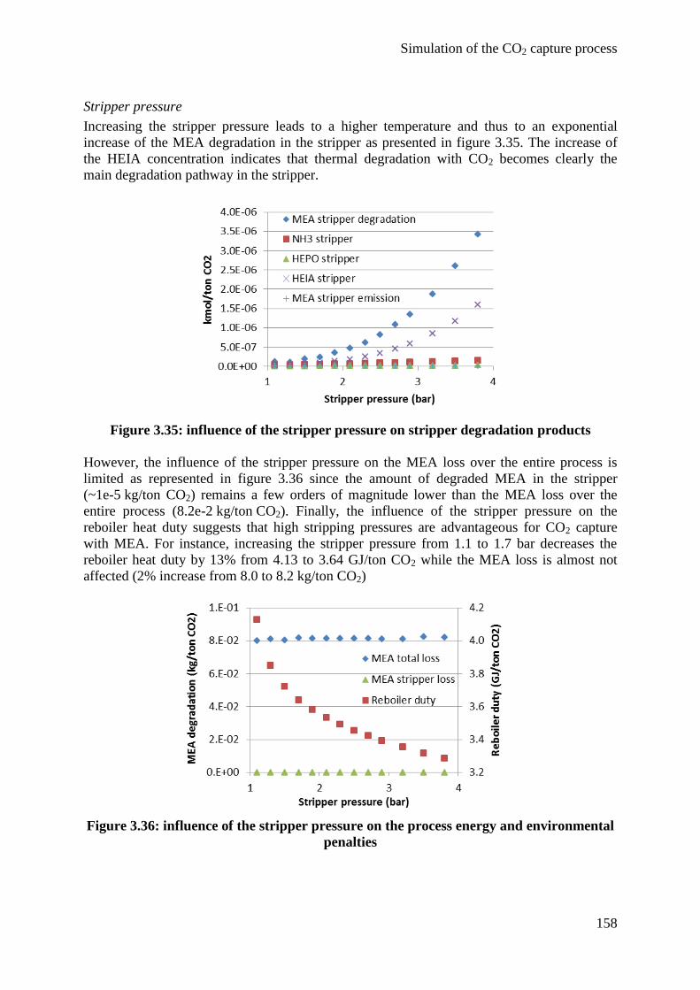
Simulation of the CO2 capture process

158

Stripper pressure

Increasing the stripper pressure leads to a higher temperature and thus to an exponential

increase of the MEA degradation in the stripper as presented in figure 3.35. The increase of

the HEIA concentration indicates that thermal degradation with CO2 becomes clearly the

main degradation pathway in the stripper.

Figure 3.35: influence of the stripper pressure on stripper degradation products

However, the influence of the stripper pressure on the MEA loss over the entire process is

limited as represented in figure 3.36 since the amount of degraded MEA in the stripper

(~1e-5 kg/ton CO2) remains a few orders of magnitude lower than the MEA loss over the

entire process (8.2e-2 kg/ton CO2). Finally, the influence of the stripper pressure on the

reboiler heat duty suggests that high stripping pressures are advantageous for CO2 capture

with MEA. For instance, increasing the stripper pressure from 1.1 to 1.7 bar decreases the

reboiler heat duty by 13% from 4.13 to 3.64 GJ/ton CO2 while the MEA loss is almost not

affected (2% increase from 8.0 to 8.2 kg/ton CO2)

Figure 3.36: influence of the stripper pressure on the process energy and environmental

penalties

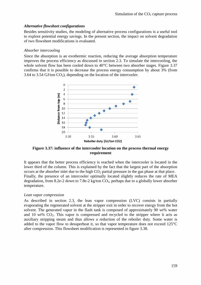
Simulation of the CO2 capture process

159

Alternative flowsheet configurations

Besides sensitivity studies, the modeling of alternative process configurations is a useful tool

to explore potential energy savings. In the present section, the impact on solvent degradation

of two flowsheet modifications is evaluated.

Absorber intercooling

Since the absorption is an exothermic reaction, reducing the average absorption temperature

improves the process efficiency as discussed in section 2.3. To simulate the intercooling, the

whole solvent flow has been cooled down to 40°C between two absorber stages. Figure 3.37

confirms that it is possible to decrease the process energy consumption by about 3% (from

3.64 to 3.54 GJ/ton CO2), depending on the location of the intercooler.

Figure 3.37: influence of the intercooler location on the process thermal energy

requirement

It appears that the better process efficiency is reached when the intercooler is located in the

lower third of the column. This is explained by the fact that the largest part of the absorption

occurs at the absorber inlet due to the high CO2 partial pressure in the gas phase at that place.

Finally, the presence of an intercooler optimally located slightly reduces the rate of MEA

degradation, from 8.2e-2 down to 7.8e-2 kg/ton CO2, perhaps due to a globally lower absorber

temperature.

Lean vapor compression

As described in section 2.3, the lean vapor compression (LVC) consists in partially

evaporating the regenerated solvent at the stripper exit in order to recover energy from the hot

solvent. The generated vapor in the flash tank is composed of approximately 90 wt% water

and 10 wt% CO2. This vapor is compressed and recycled to the stripper where it acts as

auxiliary stripping steam and thus allows a reduction of the reboiler duty. Some water is

added to the vapor flow to desuperheat it, so that vapor temperature does not exceed 125°C

after compression. This flowsheet modification is represented in figure 3.38.

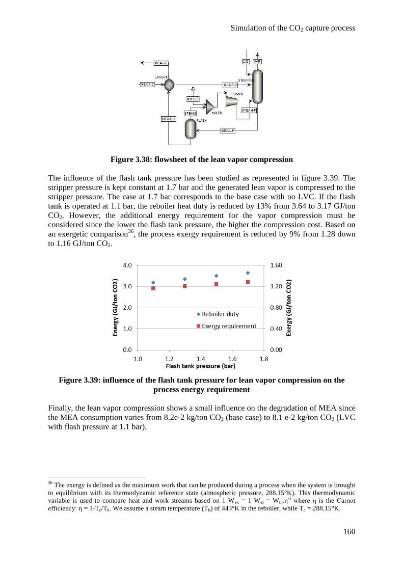
Simulation of the CO2 capture process

160

Figure 3.38: flowsheet of the lean vapor compression

The influence of the flash tank pressure has been studied as represented in figure 3.39. The

stripper pressure is kept constant at 1.7 bar and the generated lean vapor is compressed to the

stripper pressure. The case at 1.7 bar corresponds to the base case with no LVC. If the flash

tank is operated at 1.1 bar, the reboiler heat duty is reduced by 13% from 3.64 to 3.17 GJ/ton

CO2. However, the additional energy requirement for the vapor compression must be

considered since the lower the flash tank pressure, the higher the compression cost. Based on

an exergetic comparison36

, the process exergy requirement is reduced by 9% from 1.28 down

to 1.16 GJ/ton CO2.

Figure 3.39: influence of the flash tank pressure for lean vapor compression on the

process energy requirement

Finally, the lean vapor compression shows a small influence on the degradation of MEA since

the MEA consumption varies from 8.2e-2 kg/ton CO2 (base case) to 8.1 e-2 kg/ton CO2 (LVC

with flash pressure at 1.1 bar).

36

The exergy is defined as the maximum work that can be produced during a process when the system is brought

to equilibrium with its thermodynamic reference state (atmospheric pressure, 288.15°K). This thermodynamic

variable is used to compare heat and work streams based on 1 Wex = 1 Wel = Wth.η-1

where η is the Carnot

efficiency: η = 1-Tc/Th. We assume a steam temperature (Th) of 443°K in the reboiler, while Tc = 288.15°K.

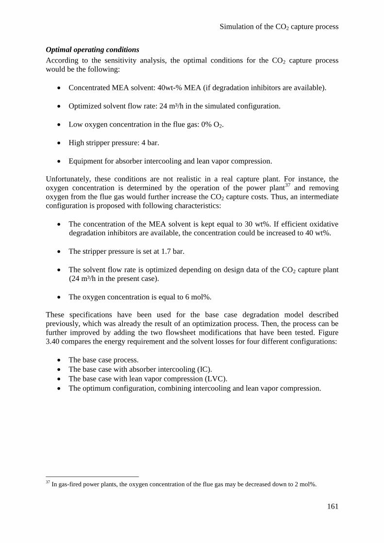
Simulation of the CO2 capture process

161

Optimal operating conditions

According to the sensitivity analysis, the optimal conditions for the CO2 capture process

would be the following:

Concentrated MEA solvent: 40wt-% MEA (if degradation inhibitors are available).

Optimized solvent flow rate: 24 m³/h in the simulated configuration.

Low oxygen concentration in the flue gas: 0% O2.

High stripper pressure: 4 bar.

Equipment for absorber intercooling and lean vapor compression.

Unfortunately, these conditions are not realistic in a real capture plant. For instance, the

oxygen concentration is determined by the operation of the power plant37

and removing

oxygen from the flue gas would further increase the CO2 capture costs. Thus, an intermediate

configuration is proposed with following characteristics:

The concentration of the MEA solvent is kept equal to 30 wt%. If efficient oxidative

degradation inhibitors are available, the concentration could be increased to 40 wt%.

The stripper pressure is set at 1.7 bar.

The solvent flow rate is optimized depending on design data of the CO2 capture plant

(24 m³/h in the present case).

The oxygen concentration is equal to 6 mol%.

These specifications have been used for the base case degradation model described

previously, which was already the result of an optimization process. Then, the process can be

further improved by adding the two flowsheet modifications that have been tested. Figure

3.40 compares the energy requirement and the solvent losses for four different configurations:

The base case process.

The base case with absorber intercooling (IC).

The base case with lean vapor compression (LVC).

The optimum configuration, combining intercooling and lean vapor compression.

37

In gas-fired power plants, the oxygen concentration of the flue gas may be decreased down to 2 mol%.

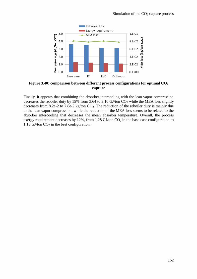
Simulation of the CO2 capture process

162

Figure 3.40: comparison between different process configurations for optimal CO2

capture

Finally, it appears that combining the absorber intercooling with the lean vapor compression

decreases the reboiler duty by 15% from 3.64 to 3.10 GJ/ton CO2 while the MEA loss slightly

decreases from 8.2e-2 to 7.8e-2 kg/ton CO2. The reduction of the reboiler duty is mainly due

to the lean vapor compression, while the reduction of the MEA loss seems to be related to the

absorber intercooling that decreases the mean absorber temperature. Overall, the process

exergy requirement decreases by 12%, from 1.28 GJ/ton CO2 in the base case configuration to

1.13 GJ/ton CO2 in the best configuration.

Simulation of the CO2 capture process

163

5. Conclusions

Most existing models of the CO2 capture process have been developed to evaluate the process

energy requirement in order to reduce the cost of the technology. However, solvent

degradation has been identified as a major issue in CO2 capture plants due to the emission of

environmentally harmful degradation products. Thus, the objective of this chapter was to

integrate the experimental results of solvent degradation previously presented into a process

model of the CO2 capture. The model is developed using the simulation tool Aspen Plus.

Before all, the main modeling aspects of the CO2 capture process with MEA have been

detailed and discussed. The Electrolyte NRTL model has been selected to evaluate fluid

properties. This model has the particularity of considering electrostatic forces due to dissolved

ions in amine solutions. Two main approaches have been tested for modeling the reactive

absorption of CO2 in mass transfer columns. The first one assumes equilibrium stages in the

columns and neglects mass transfer and chemical kinetics limitations (equilibrium

assumption). The second approach performs rigorous calculations of the reactive absorption

based on experimental data for packing hydrodynamics and chemical kinetics (rate-based

assumption).

Four different models have been developed based on design data from two different pilot

plants, the Esbjerg pilot plant developed in the framework of European CCS projects and the

so-called Mobile Pilot Unit. The first two models compare the equilibrium and the rate-based

assumptions by studying the influence of key operating parameters on the process thermal

energy requirement. It appears that both models lead to globally similar results, but the

equilibrium model systematically predicts a higher process efficiency since it neglects all

mass transfer and chemical kinetics limitations. Moreover, the rate-based model better

predicts column temperature profiles.

Then, the third model explores the potential of dynamic simulations for describing the

transient behavior of the process in transient regimes. The control of the process water

balance is improved compared to published dynamic models and the stability of the control

strategy is evaluated for different process disturbances. The process response in case of

reduced steam availability in the power plant is simulated for two different scenarios. The

scenario in which the flue gas and the solvent flow rates are kept constant at lower CO2

capture rate seems to give better results than the scenario in which the flue gas and the solvent

flow rates are decreased in the capture plant.

The fourth model includes degradation reactions based on the experimental results detailed in

Chapter II. Oxidative and thermal degradations are represented by two apparent degradation

reactions with corresponding kinetics and solvent emissions are quantified at the outlet of the

absorber and stripper washing sections. The degradation model confirms that oxidative

degradation in the absorber is by far the dominant cause for MEA loss in CO2 capture units. It

also confirms pilot plant observations that reported high NH3 emissions at the absorber outlet

as the major emission of degradation products to the environment.

Moreover, the degradation model predicts solvent consumption rates of the same order of

magnitude but slightly lower (0.082 kg/ton CO2) than those observed in pilot plants (0.284

kg/ton CO2). The lower predicted values can be explained by the modeling assumptions so

that further potential model refinements are identified:

Simulation of the CO2 capture process

164

Consideration of the influence of dissolved metals on the degradation rate.

Developing a better estimation for the oxygen solubility and transfer in amine

solutions.

Consideration of SOx and NOx-induced degradation.

Using this degradation model, the influence on solvent degradation of different key operating

variables and alternative flowsheet configurations is studied. It appears that:

An optimum value for the solvent flow rate can be identified to minimize the reboiler

heat duty. Moreover, increasing the solvent flow rate by 4 m³/h leads to a slight

increase of the MEA loss by about 1e-2 kg/ton CO2.

Increasing the MEA solvent concentration from 30 wt% to 40 wt% doubles the solvent

consumption rate from 0.082 up to 0.175 kg/ton CO2 while the reboiler heat duty is

decreased by 4 % from 3.64 to 3.50 GJ/ton CO2.

An increased O2 concentration in the flue gas from 6 mol% to 12 mol% increases the

MEA loss from 0.08 to 0.22 kg/ton CO2 while no effect on the reboiler heat duty is

observed.

Increasing the stripper pressure from 1.1 to 1.7 bar reduces the reboiler duty by 13%

with no significant increase of the MEA consumption.

The absorber intercooling and the lean vapor compression both reduce the total

process energy requirement, by 3% and 9% respectively. Moreover, they do not

significantly influence the solvent degradation.

Finally, the degradation model proposes a first approach for considering degradation reactions

as a part of the optimal design of the CO2 capture process. A methodology implying

experimental degradation studies and process modeling tools has been proposed based on the

benchmark solvent 30wt% MEA, and further model improvements have been identified.

Conclusions and perspectives

165

Chapter IV

Conclusions and perspectives

“If you do not change direction, you may end up where you are heading.”

Lao Tzu

Conclusions and perspectives

166

1. Conclusions

Environmental concern has received an increased attention in the last few decades as the

scientific community has warned about the effects of anthropogenic greenhouse gas emissions

on the environment. In this context, CO2 capture and storage technologies are proposed as one

of the potential contributions to a decarbonated energy mix. Their objective is to capture the

CO2 emitted during the combustion of fossil fuels and to re-use it or to store it underground.

In the present work, the post-combustion CO2 capture with amine solvents is studied. It is the

most mature CO2 capture technology for large-scale applications like coal or natural gas-fired

power plants. Moreover, this technique can be used to retrofit existing plants by treating the

flue gas after combustion. However, two main drawbacks slow down the development of

post-combustion capture:

The high energy requirement of the process for regenerating the amine solvent that has

absorbed CO2.

The environmental impact related to the emission of amine solvents and degradation

products into the atmosphere.

Both of these aspects are usually studied separately. In the present work, they are combined in

a multi-disciplinary approach. Indeed, a methodology is developed to simultaneously evaluate

the influence of process operating parameters on the process energy requirement and on the

degradation of amine solvents. This study considers an aqueous solution of

monoethanolamine (MEA), which is the benchmark solvent for post-combustion CO2 capture.

In a first phase, the influence of several process operating parameters on the solvent

degradation is quantified. Both experimental degradation test rig with continuous gas flow

and batch degradation cylinders are used to study the two main degradation pathways of

MEA, i.e. the oxidative degradation and the thermal degradation with CO2. Moreover,

appropriate analytical techniques are developed to characterize solvent degradation by

quantifying the amine content and the formation of liquid and vapor degradation products.

The principal conclusions of this experimental study are the following:

Similar degradation pathways and products are observed in the degradation test rig

compared with CO2 capture pilot plants.

Solvent degradation in CO2 capture plants is essentially caused by the oxidative

degradation of MEA.

The rate of oxidative degradation is determined by the oxygen mass transfer between

the flue gas and the liquid solvent. Different factors affect the oxygen mass transfer,

and thus the rate of oxidative degradation:

- The agitation rate,

- The oxygen concentration in the flue gas,

- The presence of CO2 in the amine,

- The temperature.

Conclusions and perspectives

167

Dissolved metals catalyze the oxidative degradation but show no influence on the

thermal degradation with CO2.

Inhibitors of the oxidative degradation may successfully prevent MEA degradation.

The rate of thermal degradation with CO2 is affected by the temperature and the

presence of CO2. Moreover, some oxidative degradation inhibitors decrease the

thermal stability of amine solutions.

In a second phase, a simulation model of the process has been developed using the software

package Aspen Plus. Different modeling approaches are considered and compared for the

post-combustion CO2 capture with MEA. The main results of this modeling study are listed

below:

The limitations of a simplified model that assumes ideal mass transfer and

instantaneous chemical reactions have been evidenced, especially for the prediction of

column temperature profiles. This model is compared with a rigorous rate-based

model by studying the influence of different process parameters on the reboiler duty.

The potential of dynamic modeling for predicting the behavior of the CO2 capture

process in transient operating mode has been evidenced. An efficient control strategy

has been developed and two scenarios for a rapid reduction of the energy requirement

of the capture plant have been studied.

Finally, a kinetic model of solvent degradation considering oxidative and thermal degradation

of MEA with CO2 has been developed based on the results of degradation experiments. This

model has been included in a global model of the CO2 capture process using a detailed rate-

based approach for the calculation of mass transfer and chemical reactions. The main

observations reported for this model are the following:

The model confirms that oxidative degradation in the absorber is the main cause for

solvent loss in CO2 capture plants. It also confirms that ammonia emissions at the

absorber outlet are one of the major environmental issues.

The influence of process operating variables on the energy and the environmental

penalties of the CO2 capture process is quantified. The solvent flow rate and

concentration, the stripper pressure and the oxygen concentration in the flue gas are

varied. The largest energy savings are observed by increasing the stripper pressure and

the solvent concentration, while the most significant increases of the MEA

consumption are due to the increased oxygen concentration in the flue gas and to the

higher solvent concentration.

Two process improvements have been tested. The absorber intercooling and the lean

vapor compression both reduce the total process energy requirement with no

significant influence on solvent degradation. Combining these two improvements

allows a reduction of the process energy requirement by 12%.

This kind of model could and should be used for the design of CO2 capture plants to consider

not only the process energy penalty, but also its environmental penalty which is particularly

relevant for large-scale applications.

Conclusions and perspectives

168

2. Perspectives

In the framework of this new research subject, different experimental and modeling tools have

been developed at the University of Liège. However, numerous questions have been raised

during the present study that would require further investigations. Similarly, many

assumptions have been made for modeling solvent degradation in a first approach, and there

is room for significant improvements of the resulting degradation model. Among others,

following assumptions could be refined:

The influence of dissolved metals on MEA degradation has been observed, but the

kinetic models have been developed based on metal-free solutions. Studying the

influence of process operating parameters in the presence of dissolved metals should

lead to a more precise modeling of solvent degradation.

The calculation of dissolved oxygen concentrations in the amine solutions is based on

the assumption of oxygen saturation. However, experimental results evidence that

oxidative degradation is limited by the oxygen transfer. Thus, a better description of

the oxygen solubility would certainly improve the precision of the model.

The influence of flue gas contaminants like SOx and NOx on the degradation of MEA

has not been considered. This could be the object of further experimental and

modeling works.

The influence of the MEA concentration on solvent degradation has been neglected.

This assumption could be verified by experimental tests in the Degradation Test Rig.

The activation energy of the oxidative degradation has been measured in the presence

of CO2. Measurements of the oxidative degradation rate at different temperatures and

in the absence of CO2 could refine the estimation of the activation energy for the

oxidative degradation of MEA.

The model describing the thermal degradation of MEA with CO2 is very basic. It

could be refined by using the degradation kinetics proposed by Davis (2009).

Alternatively, more tests could be performed in batch cylinders in order to get more

experimental data for the model development.

The influence of CO2 has been considered in a basic way, assuming that the amines

solutions were either loaded with CO2 or unloaded. Studying the effect of process

operating parameters at various solvent loading could improve the comprehension of

the CO2 inhibiting effect. However, an analytic method should be developed for that

specific purpose since the loading of degraded amine solutions cannot be determined

precisely by usual analytical methods.

The proposed degradation model has not been validated against pilot plant data. This

could be a further improvement of the model in order to precisely evaluate the process

energy requirement and the emissions of amine solvent and degradation products.

Conclusions and perspectives

169

The potential of dynamic simulations has been evidenced with an equilibrium model.

Further developments could include a rate-based approach for the mass transfer

calculations in dynamic mode.

However, the most important development proposed in this work is not the degradation model

on itself, but rather the methodology that has been applied to develop this model. The

experimental, analytic and modeling procedures that have been presented in the present study

can be easily transposed to other solvent systems since many studies focus on developing

alternative solvent to MEA. For instance, piperazine appears as a promising solvent for post-

combustion CO2 capture, so that a process model including solvent degradation could be

developed for piperazine. Solvent blends also offer interesting perspectives, as well as

demixing solvents.

Finally, a further important improvement would be to consider the impact of solvent

degradation on solvent properties, and thus on the operation of the CO2 capture process. For

instance, preliminary tests performed at the University of Liège have shown that the viscosity

of a degraded MEA solution increases by about 5% compared to the fresh solvent. Other

solvent properties may also be influenced by the presence of degradation products so that the

performances of the CO2 capture process may be significantly affected. This is also the case

for the corrosivity of the solvent solution, which increases in the presence of degradation

products. As a consequence, quantifying the effects of degradation on solvent properties

would help to reduce the technology drawbacks and further contribute to the large-scale

development of the CO2 capture.

Bibliography

170

Bibliography

Abanades JC, Anthony E.J., Lu D.Y., Salvador C., Alvarez D., 2004. Capture of CO2 from

Combustion Gases in a Fluidized Bed of CaO. AiCHE Journal 50 (7), 1614-1622.

Abu-Zahra M., Schneiders L., Niederer J., Feron P., Versteeg G., 2007. CO2 capture from

power plants. Part I. A parametric study of the technical performance based on

monoethanolamine. International Journal of Greenhouse Gas Control 1, 37-46.

Abu-Zahra M., Schneiders L., Niederer J., Feron P., Versteeg G., 2007. CO2 capture from

power plants. Part II. A parametric study of the economical performance based on mono-

ethanolamine. International Journal of Greenhouse Gas Control 1, 135-142.

Abu-Zahra M., 2009, Carbon dioxide capture from flue gas, PhD Thesis at Delft University,

The Netherlands.

ADEME, 2010. Panorama des voies de valorisation du CO2. Agence de l'Environnement et de

la Maîtrise de l'Energie, France.

Ahmadi A., 2011. Modélisation de l'absorption réactive multiconstituant : application au

traitement des gaz acides par des solvants aux alcanolamines. PhD Thesis at the University of

Toulouse (INP Toulouse), France.

Aroonwilas V., 2005. Evaluation of split-flow scheme for CO2 absorption process using

mechanistic mass-transfer and hydrodynamic model. Proceedings of the 7th International

Conference on Greenhouse Gas Control Technologies 5, 1841-1844.

Aspentech, 2008. Rate-based model of the CO2 capture process by MEA using Aspen Plus.

Aspen Plus V7.0 support files.

Aspentech, 2012. Rate-based model of the CO2 capture process by MEA using Aspen Plus.

Aspen Plus V8.0 support files.

Astarita G., Savage D., Bisio A., 1983. Gas Treating with Chemical Solvents. Wiley, New

York.

Austgen D., 1989. A model of vapor-liquid equilibria for acid gas-alkanolamine-water

systems. PhD Thesis, University of Texas at Austin, USA.

Austgen D., Rochelle G., Peng X., Chen C.C., 1989. Model of Vapor-Liquid Equilibria for

Aqueous Acid Gas-Alkanolamine Systems Using the Electrolyte-NRTL Equation. Ind. Eng.

Chem. Res. 28, 1060-1073.

Bailey D., P. Feron, 2005. Post-combustion Decarbonisation Processes, Oil & Gas Science

and Technology 60 (3), 461-474.

Barchas, R. and R. Davis, 1992. The Kerr-McGee/ABB Lummus Crest Technology for the

recovery of CO2 from stack gases. Energy Conversion Management, 33 (5-8), 333-340.

Bibliography

171

Barker D., Turner S., Napier-Moore P., Clark M., Davison J., 2009. CO2 Capture in the

Cement Industry. Energy Procedia 1, 87-94.

Bascougnano M., 2012. Développement d’une méthode analytique pour l’étude de la

dégradation de la 2-éthanolamine dans le cadre d’un procédé de capture de CO2. Internship

report. University of Liège, Belgium.

Bedell S., 2009, Oxidative degradation mechanisms for amine in flue gas capture, Energy

Procedia 1, 771–778.

Bedell S., 2011. Amine autoxidation in flue gas CO2 capture—Mechanistic lessons learned

from other gas treating processes. International Journal of Greenhouse Gas Control 5, 1–6.

Bello A., Idem R., 2005. Pathways for the Formation of Products of the Oxidative

Degradation of CO2-Loaded Concentrated Aqueous Monoethanolamine Solutions during CO2

Absorption from Flue Gases. Ind. Eng. Chem. Res. 44, 945-969.

Bello A., Idem R., 2006. Comprehensive Study of the Kinetics of the Oxidative Degradation

of CO2 Loaded and Concentrated Aqueous Monoethanolamine (MEA) with and without

Sodium Metavanadate during CO2 Absorption from Flue Gases. Ind. Eng. Chem. Res. 45,

2569-2579.

Bellona, 2007. Factsheet : CO2 capture. The Bellona Foundation. www.bellona.org, accessed

in March 2013.

Bellona, 2013. CO2 capture. Bellona environmental CCS team. www.bellona.org, accessed in

March 2013.

Benson H., McCrea D., 1979. Emoval of acid gases from hot gas mixtures. US Patent

4160810.

Billet R., Schultes M., 1993. Predicting mass transfer in packed columns. Chemical

Engineering and Technology 16, 1–9.

Billet R., Schultes M., 1999. Prediction of mass transfer columns with dumped and arranged

packings. Updated summary of the calculation method of Billet and Schultes. Chem. Eng.

Res. Des. 77, 498–504.

Blachly C. and Ravner H., 1965a. The Stabilization of Monoethanolamine Solutions for

Submarine Carbon Dioxide Scrubbers. Report 6189, U.S. Naval Research Laboratory.

Blachly C. and Ravner H., 1965b. Studies of Submarine Carbon Dioxide Scrubber Operation:

Effect of an Additive Package for the Stabilization of Monoethanolamine Solutions. Report

1598, U.S. Naval Research Laboratory.

Bollas G., Chen C., Barton P., 2008. Refined Electrolyte-NRTL Model: Activity Coefficient

Expressions for Application to Multi-Electrolyte Systems. AIChE Journal vol. 54 (6), 1608-

1624.

Bibliography

172

Bravo J., Fair J., 1982. Generalized correlation for mass transfer in packed distillation

columns, Ind. Eng. Chem. Process Des. Dev. 21, 162.

Bravo J., Rocha J., Fair J., 1985. Mass-transfer in Gauze packings. Hydrocarbon Process 64,

91–95.

Bravo J., Rocha J., Fair J., 1992. A comprehensive model for the performance of columns

containing structured packings. I. ChemE. Symp. Ser. 129, A439.

Brúder P., Svendsen H., 2012. Capacity and kinetics of solvents for post-combustion CO2

Capture. Energy Procedia 23, 45 – 54.

Captech, 2007. Openbaareindrapport Captech jaar 1 (2006-2007), Advanced Solvents.

www.co2-captech.nl, accessed in January 2010.

Captech, 2008. Advanced Solvent Development at Shell, 2nd CAPTECH Day, Arnhem, 06.

March 2008.

Cato, 2012. Dutch national research and development program for CO2 capture, transport and

storage. www.co2-cato.org, accessed in February 2012.

Cesar, 2012. CO2 enhanced separation and recovery. Project co-founded by the 7th

framework

program of the European Commission. www.co2cesar.eu, accessed in February 2012.

Chakma A., 1997. CO2 capture processes – Opportunities for improved energy efficiencies.

Energy Conversion Management 38, 51-56.

Challis B., Challis J., 1982. N-nitrosamines and N-nitrosimines. In: Patai, S., ed., The

Chemistry of Amino, Nitroso and Nitro Compounds and Their Derivatives, Wiley, New York,

1151-1223.

Chanchey A., Saiwan C., Supap T., Idem R., Tontiwachwuthikul P., 2011. Off-Gas Emission

in CO2 Capture Process Using Aqueous Monoethanolamine Solution. Energy Procedia 4,

504–511.

Chapel D., Mariz C., Ernest J., 1999. Recovery of CO2 from Flue Gases: Commercial Trends.

Presentation at the Canadian Society of Chemical Engineers annual meeting, Saskatchewan,

Canada.

Chen C.C., Britt H.I., Boston J.F., Evans L.B., 1982. Local Compositions Model for Excess

Gibbs Energy of Electrolyte Systems: Part I: Single Solvent, Single Completely Dissociated

Electrolyte Systems. AIChE Journal 28 (4), 588-596.

Chen C.C., Evans L., 1986. A local Composition Model for the Excess Gibbs Energy of

Aqueous Electrolyte Systems. AIChE Journal 32 (3), 444-454.

Chen C.C., 2006. Toward development of activity coefficient models for process and product

design of complex chemical systems. Fluid Phase Equilibria 241, 103–112.

Bibliography

173

Chi S., Rochelle, G., 2001. Oxidative Degradation of Monoethanolamine. Master Thesis,

University of Texas at Austin, USA.

Chi S., Rochelle G., 2002. Oxidative Degradation of Monoethanolamine. Ind. Eng. Chem.

Res. 41, 4178-4186.

Ciferno J., Di Pietro P., Tarka T., 2005. An economic scoping study for CO2 capture using

aqueous ammonia. Final Report - DOE/NETL

CO2 capture project, 2008. Three basic methods to separate gases.

www.co2captureproject.org/pdfs/3_basic_methods_gas_separation.pdf, accessed in April

2013.

CO2 capture project, 2013. CO2 Storage: Operation - injecting CO2 underground

www.co2captureproject.org/operation.html, accessed in April 2013.

Cook P.J., 2009. Demonstration and Deployment of Carbon Dioxide Capture and Storage in

Australia. Energy Procedia 1, 3859-3866.

Cooper C. on behalf of the CO2 capture project, 2009. A technical basis for carbon dioxide

storage. Energy Procedia 1, 1727-1733.

Cousins A., Wardhaugh L., Feron P., 2011. Preliminary analysis of process flow sheet

modifications for energy efficient CO2 capture from flue gases using chemical absorption.

Chemical Engineering Research and Design 89, 1237–1251.

CSLF, 2011. In Focus: what is carbon utilization. Carbon sequestration leadership forum.

www.cslforum.org, accessed in April 2013.

Cummings A., Smith G., Nelsen D., 2007. Advances in Amine Reclaiming - Why There's No

Excuse to Operate a Dirty Amine System. Proceedings of the Laurance Reid gas conditioning

conference, 227-244.

Danckwerts A.W., 1951. Significance of liquid film coefficient in gas absorption. Ind. Eng.

Chem. 43, 1460-1467.

Danckwerts P.V., 1979. The reaction of CO2 with ethanolamines. Chem. Eng. Sci. 34 (4),

443-446, 1979.

Davis J., 2009. Thermal Degradation of Aqueous Amines Used for Carbon Dioxide Capture.

PhD Thesis, University of Texas at Austin, USA.

Davis J., Rochelle, G., 2009. Thermal degradation of monoethanolamine at stripper

conditions. Energy Procedia 1, 327-333.

de Koeijer G., Enge Y., Sanden K., Graff O.F., Falk-Pedersenc O., Amundsen T., Overå S.,

2011. CO2 Technology Centre Mongstad – Design, Functionality and Emissions of the Amine

Plant. Energy proceedia 4, 1207-1213.

Bibliography

174

Delfort B., Carrette P.-L., Bonnard L., 2011. MEA 40% with Improved Oxidative Stability

for CO2 Capture in Post-Combustion. Energy Procedia 4, 9-14.

Deshmukh R., Mather A., 1981. A Mathematical Model for Equilibrium Solubility of

Hydrogen Sulfide and Carbon Dioxide in Aqueous Alkanolamine Solutions. Chemical

Engineering Science 36, 355-362.

Dow, 2003. Material safety data sheet for ethanolamines.

http://msdssearch.dow.com/PublishedLiteratureDOWCOM/dh_017d/0901b8038017d302.pdf

?filepath=amines/pdfs/noreg/111-01375.pdf&fromPage=GetDoc, accessed in April 2013.

Dubois L., Thomas D., 2009. CO2 Absorption into Aqueous Solutions of Monoethanolamine,

Methyldiethanolamine, Piperazine and their Blends. Chem. Eng. Technol. 32 (5), 1–10.

Dubois L., 2013. Etude de la capture du CO2 en postcombustion par absorption dans des

solvants aminés : application aux fumées issues de cimenteries. PhD thesis at the University

of Mons, Belgium.

Dugas R., Alix P., Lemaire E., Broutin P., Rochelle G., 2009. Absorber model for CO2

capture by monoethanolamine – application to CASTOR pilot results. Energy procedia 1,

103-107.

Endo T., Kajiya Y., Nagayasu H., Iijima M., Ohishi T., Tanaka H., Mitchell R., 2011. Current

status of MHI’s CO2 recovery technology and optimization of CO2 recovery plant with a PC

fired power plant. Energy Procedia 4, 1513–1519.

Engebo A., Ahmed N., Rose E., Helle K., Hage L.J., 2012. Report activity 5: CO2 transport.

Det Norske Veritas, Report No 2012-0076 for Gassnova SF.

Epp B., Fahlenkamp H., Vogt M., 2011. Degradation of solutions of monoethanolamine,

diglycolamine and potassium glycinate in view of tail-end CO2 absorption. Energy Procedia

4, 75-80.

Faramarzi L, Kontogeorgis G., Michelsen M., Thosen K., Stenby E., 2010. Absorber Model

for CO2 Capture by Monoethanolamine. Ind. Eng. Chem. Res. 49, 3751–3759.

Fluxys, 2013. Stockage de gas naturel: le site de Loenhout. www.fluxys.be accessed in

February 2013.

Figueroa J., Fout T., Plasynski S., McIlvried H., Srivastava R., 2008. Advances in CO2

capture technology—The U.S. Department of Energy’s Carbon Sequestration Program.

International journal of greenhouse gas control 2, 9–20.

Fostås B., Gangstad A., Nenseter B., Pedersen S., Sjovoll M. et Sorensen A., 2011. Effects of

NOx in the Flue Gas Degradation of MEA. Energy Procedia 4, 1566-1573.

Fouad W., Berrouk A., Peters C., 2012. Improved Kent-Eisenberg models for predicting H2S

and CO2 solubilities in aqueous TEA solutions. Proceedings of the 3rd

International Gas

Processing Symposium, March 5 - 7 2012, Qatar.

Bibliography

175

Freguia S., Rochelle G., 2003. Modeling of CO2 Capture by Aqueous Monoethanolamine.

AIChE Journal 49 (7), 1676-1686.

Fürst W., Renon H., 1993. Representation of Excess Properties of Electrolyte Solutions Using

a New Equation of State. AIChE Journal 39 (2), 335-343.

Gabrielsen J., Michelsen M., Stenby E., Kontogeorgis G., 2005. A Model for Estimating CO2

Solubility in Aqueous Alkanolamines. Ind. Eng. Chem. Res. 44, 3348-3354.

Gaspar J., Cormos A-M., 2012. Dynamic modeling and absorption capacity assessment of

CO2 capture process. International Journal of Greenhouse Gas Control 8, 45–55.

Goff G., Rochelle G., 2003. Oxidative degradation of aqueous monoethanolamine in CO2

capture systems under absorber conditions. Greenhouse Gas Control Technologies 1, 115-

120.

Goff G., Rochelle G., 2004. Monoethanolamine Degradation: O2 Mass Transfer Effects under

CO2 Capture Conditions. Ind. Eng. Chem. Res. 43, 6400-6408.

Goff G., 2005. Oxidative degradation of aqueous MEA in CO2-capture processes: Iron and

copper catalysis, Inhibition and O2 mass transfer. PhD Thesis at the University of Texas at

Austin, USA.

Goff G., Rochelle G., 2006. Oxidation Inhibitors for Copper and Iron Catalyzed Degradation

of Monoethanolamine in CO2 Capture Processes. Ind. Eng. Chem. Res. 45, 2513-2521.

Gross J., and Sadowski G., 2001. Perturbed-Chain SAFT: An Equation of State Based on a

Perturbation Theory for Chain Molecules. Ind. Eng. Chem. Res. 40, 1244-1260.

Guggenheim E., 1935. The specific thermodynamic properties of aqueous solutions of strong

electrolytes. Phil. Mag. 19, 588-643.

Harun N., Douglas P., Ricardez-Sandoval L., Croiset E., 2011. Dynamic Simulation of MEA

Absorption Processes for CO2 Capture from Fossil Fuel Power Plant. Energy Procedia 4,

1478–1485.

David J. Heldebrant, Clement R. Yonker, Philip G. Jessop, Lam Phan, 2009. CO2-binding

organic liquids (CO2BOLs) for post-combustion CO2 Capture. Energy Procedia 1, 1187-1195.

Hessen E., Haug-Warberg T., Svendsen H., 2010. The refined e-NRTL model applied to

CO2–H2O–alkanolamine systems. Chemical Engineering Science 65, 3638–3648.

Higbie R., 1935. The rate of absorption of a pure gas into a still liquid during short periods of

exposure. Trans. Am. Inst. Chem. Ing. 31, 365.

Hikita H., Asai S., Ishikawa H., Honda M., 1977. The Kinetics of Reactions of Carbon

Dioxide with Monoethanolamine, Diethanolamine, and Triethanolamine by a Rapid Mixing

Method. Chemical Engineering Journal 13 (1), 7-12.

Bibliography

176

Hoff K., Juliussen O., Falk-Pedersen O., and Svendsen H., 2004. Modeling and Experimental

Study of Carbon Dioxide Absorption in Aqueous Alkanolamine Solutions Using a Membrane

Contactor. Ind. Eng. Chem. Res. 43, 4908-4921.

Huizeling E. and van der Weijde G., 2011. ROAD Maasvlakte CCS Project C.V., Non-

confidential FEED study report – Special report for the Global Carbon Capture and Storage

Institute. www.globalccsinstitute.com, accessed in February 2013.

Idem R., Wilson M., Tontiwachwuthikul P., Chakma A., Veawab A., Aroonwilas A.,

Gelowitz D., 2006. Pilot Plant Studies of the CO2 Capture Performance of Aqueous MEA and

Mixed MEA/MDEA Solvents at the University of Regina CO2 Capture Technology

Development Plant and the Boundary Dam CO2 Capture Demonstration Plant. Ind. Eng.

Chem. Res. 45, 2414-2420.

IEA, 2008. CO2 capture and storage: a key carbon abatement option. International energy

agency, 2008.

IEO, 2011. International Energy outlook 2011, US energy information administration,

http://www.eia.gov/forecasts/ieo/, accessed in 2012.

IPCC, 2005. IPCC special report on carbon dioxide capture and storage. Prepared by working

group III of the Intergovernmental Panel on Climate Change. Cambridge university press,

Cambridge, NY, USA.

Jamal A., Meisen A., Lim C., 2006. Kinetics of carbon dioxide absorption and desorption in

aqueous alkanolamine solutions using a novel hemispherical contactor - I. Experimental

apparatus and mathematical modeling. Chemical Engineering Science 61, 6571 – 6589.

Jassim M., Rochelle G., 2006. Innovative Absorber/Stripper Configurations for CO2 Capture

by Aqueous Monoethanolamine. Ind. Eng. Chem. Res. 45, 2465-2472.

Jockenhövel T., Schneider R., Rode H., 2009a. Development of an Economic Post-

Combustion Carbon Capture Process. Energy Procedia 1, 1043-1050.

Jockenhövel T., Schneider R., Sandell M., Schlüter L., 2009b. Optimal Power Plant

Integration of Post-Combustion CO2 Capture. POWER-GEN Europe 2009 – Cologne,

Germany.

Jou F., Mather A. , Otto F. , 1982. Solubility of Hydrogen Sulfide and Carbon Dioxide in

Aqueous Methyldiethanolamine Solutions. Ind. Eng. Chem. Process Des. Dev. 21 (4), 539-

544.

Jou F., Carroll J., Mather A., Otto F., 1993a. Solubility of Mixtures of Hydrogen Sulfide and

Carbon Dioxide in Aqueous N-Methyldiethanolamine Solutions. J. Chem. Eng. Data 38 (1),

75-77.

Jou F., Carroll J., Mather A., Otto F., 1993b. The Solubility of Carbon Dioxide and Hydrogen

Sulfide in a 35 wt% Aqueous Solution of Methyldiethanolamine. The Canadian Journal of

Chemical Engineering 71 (2), 264-268.

Bibliography

177

Kaminski M., Jastrzebski D., Przyjazny A., Kartanowicz R., 2002. Determination of the

Amount of Wash Amines and Ammonium Ion in Desulfurization Products of Process Gases

and Results of Related Studies. J. Chromatogr. A 947, 217-225.

Karimi M., Hillestad M., Svendsen H., 2011a. Investigation of intercooling effect in CO2

capture energy consumption. Energy Procedia 4, 1601–1607.

Karimi M., Hillestad M., Svendsen H., 2011b. Capital costs and energy considerations of

different alternative stripper configurations for post combustion CO2 capture. Chemical

Engineering Research and Design 89, 1229–1236.

Karimi M., Hillestad M., Svendsen H., 2012. Investigation of the dynamic behavior of

different stripper configurations for post-combustion CO2 capture. International Journal of

Greenhouse Gas Control 7, 230-239.

Kenig E., Schneider R., Górak A., 2001. Reactive absorption: Optimal process design via

optimal modelling. Chemical engineering science 56, 343-350.

Kent R., Eisenberg B, 1976. Better Data for Amine Treating. Hydrocarbon Processing 55 (2),

87-90.

Knudsen J., Jensen J., Vilhelmsen P., Biede O., 2007. First year operation experience with a

1 t/h CO2 absorption pilot plant at Esbjerg coal-fired power plant. Proceedings of European

Congress of Chemical Engineering (ECCE-6) Copenhagen, 16-20 September 2007.

Knudsen J., Vilhelmsen P., Jensen J., Biede O., 2009. Experience with CO2 capture from coal

flue gas in pilot scale. Energy Procedia 1, 783-790.

Knudsen J., Andersen J., Jensen J., Biede O., 2011. Evaluation of process upgrades and novel

solvents for the post combustion CO2 capture process in pilot-scale. Energy Procedia 4, 1558–

1565.

Krishna R., Standart G., 1976. A Multicomponent Film Model Incorporating a General

Matrix Method of Solution to the Maxwell-Stefan Equations. AIChE Journal 22 (2), 383-389.

Kucka L., Richter J., Kenig E., Gorak A., 2003. Determination of Gas-Liquid Reaction

Kinetics with a Stirred Cell Reactor. Sep. Purif.Technol. 31, 163–175.

Kumar A., 1982. Kinetics of complexation and oxidation of ethanolamine and diols by silver

(II). J. Phys. Chem. 86, 1674-1678.

Kvamsdal H., Jakobsen J., Hoff K., 2009. Dynamic modeling and simulation of a CO2

absorber column for post-combustion CO2 capture. Chemical Engineering and Processing 48,

135–144.

Kvamsdal H., Hetland J., Haugen G., Svendsen H., Major F., Kårstad V., Tjellander G., 2010.

Maintaining a neutral water balance in a 450MWe NGCC-CCS power system with post-

combustion carbon dioxide capture aimed at offshore operation. International Journal of

Greenhouse Gas Control 4, 613–622.

Bibliography

178

Kvamsdal H., Haugen G., Svendsen H., 2011a. Flue-gas cooling in post-combustion capture

plants. Chemical Engineering Research and Design 89, 1544–1552.

Kvamsdal H., Haugen G., Svendsen H., Tobiesen A., Mangalapally H., Hartono A., Mejdell

T., 2011b. Modelling and simulation of the Esbjerg pilot plant using the Cesar 1 solvent.

Energy Procedia 4, 1644–1651.

Laborelec, 2009. Discussions with the industrial partner, Sustainable Process Technologies

group.

Lam M.K., Lee K.T., Mohamed A.R., 2012. Current status and challenges on microalgae-

based carbon capture. International Journal of Greenhouse Gas Control 10, 456–469.

Lawal A., Idem R., 2005. Effects of Operating Variables on the Product Distribution and

Reaction Pathways in the Oxidative Degradation of CO2- Loaded Aqueous MEA-MDEA

Blends during CO2 Absorption from Flue Gas Streams. Ind. Eng. Chem. Res. 44, 986-1003.

Lawal A., Bello A. and Idem R., 2005, The Role of Methyl Diethanolamine (MDEA) in

Preventing the Oxidative Degradation of CO2 Loaded and Concentrated Aqueous

Monoethanolamine (MEA)-MDEA Blends during CO2 Absorption from Flue Gases. Ind.

Eng. Chem. Res. 44, 1874-1896.

Lawal A. and Idem R., 2006. Kinetics of the Oxidative Degradation of CO2 Loaded and

Concentrated Aqueous MEA-MDEA Blends during CO2 Absorption from Flue Gas Streams,

Ind. Eng. Chem. Res. 45, 2601-2607.

Lawal A., Wang M., Stephenson P., 2011. Investigating the dynamic response of CO2

chemical absorption process in enhanced-O2 coal power plant with post-combustion CO2

capture. Energy Procedia 4, 1035–1042.

Lemaire E., Bouillon P.A., Gomez A. Kittel J., Gonzales S., Carrette P.L., Delfort B., Ougin

P., Alix P., Normand L., 2011. New IFP optimized first generation process for post-

combustion CO2 capture: HiCapt+TM

. Energy Procedia 4, 1361-1368.

Léonard G., Heyen G., 2011a. Modeling post-combustion CO2 capture with amine solvents.

Computer Aided Chemical Engineering 29, 1768-1772.

Léonard G., Heyen G., 2011b. Optimisation du procédé de captage de CO2 dans des solvants

aminés. Récents Progrès en Génie des Procédés, 101.

Lepaumier H., 2008. Etude des mécanismes de dégradation des amines utilisées pour le

captage du CO2 dans les fumées. PhD thesis at the University of Savoie, France.

Lepaumier H., Picq D., Carrette P., 2009a. Degradation Study of new solvents for CO2

capture in post combustion. Energy Procedia 1, 893-900.

Lepaumier H., Picq D., Carrette P., 2009b. New Amines for CO2 Capture. I. Mechanisms of

Amine Degradation in the Presence of CO2. Ind. Eng. Chem. Res. 48, 9061–9067.

Bibliography

179

Lepaumier H., Picq D., Carrette P., 2009c. New Amines for CO2 Capture. II. Oxidative

Degradation Mechanisms. Ind. Eng. Chem. Res. 48, 9068–9075.

Lepaumier H., da Silva E., Einbu A., Grimstvedt A., Knudsen J., Vernstad K., Zahlsen K.,

Svendsen H., 2010. Comparison of MEA degradation in pilot-scale and lab-scale

experiments. Presentation at the 10th

international conference on greenhouse gas technologies

conference, Amsterdam, The Netherlands.

Lepaumier H., da Silva E., Einbu A., Grimstvedt A., Knudsen J., Zahlsen K., Svendsen H.,

2011. Comparison of MEA degradation in pilot-scale with lab-scale experiments. Energy

Procedia 4, 1652–1659.

Lepaumier H., 2011. Informal discussion. Laborelec, Sustainable Process Technologies

group.

Lin Y-J., David Wong D., Jang S-S., 2011. Control Strategies for Flexible Operation of

Power Plant with CO2 Capture Plant. AIChE Journal 58 (9), 2697-2704.

Luo X., Knudsen J., de Montigny D., Sanpasertparnich T., Idem R., Gelowitz D., Notz R.,

Hoch S., Hasse H., Lemaire E., Alix P., Tobiesen A., Juliussen O., Köpcke M., Svendsen H.,

2009. Comparison and validation of simulation codes against sixteen sets of data from four

different pilot plants. Energy Procedia 1, 1249-1256.

Majer V., Sedlbauer J., Bergin G., 2008. Henry’s law constant and related coefficients for

aqueous hydrocarbons, CO2 and H2S over a wide range of temperature and pressure. Fluid

Phase Equilibria 272, 65–74.

McCalley D., 2007. Is hydrophilic interaction chromatography with silica columns a viable

alternative to reversed-phase liquid chromatography for the analysis of ionisable compounds?

Journal of Chromatography A 1171, 46–55.

Mejdell T., Vassbotn T., Juliussen O., Tobiesen A., Einbu A., Knuutila H., Hoff K.,

Andersson V., Svendsen H., 2011. Novel full height pilot plant for solvent development and

model validation. Energy Procedia 4, 1753–1760.

Meldon J., Morales-Cabrera M., 2011. Analysis of carbon dioxide absorption in and stripping

from aqueous monoethanolamine. Chemical Engineering Journal 171, 753– 759.

Meng L., 2004. Development of an Analytical Method for Distinguishing Ammonium

Bicarbonate from the Products of an Aqueous Ammonia CO2 Scrubber and the

Characterization of Ammonium Bicarbonate. Masters Theses & Specialist Projects.

Department of Chemistry, Western Kentucky University.

MHI, 2012. Press Information, Mitsubishi Heavy Industries. World's First Integrated CCS of

Coal-fired Power Plant Emissions Begins 500 tons/day Joint Demonstration Project with

Southern Company. www.mhi.co.jp/en/news/story/1209141573.html, accessed in April 2013.

Mimura T., Shimojo S., Suda T., Iijima M., Mitsuoka S., 1995. Research and development on

energy saving technology for flue gas carbon dioxide recovery and steam system in power

plant. Energy Conversion Management 36 (6-9), 397-400.

Bibliography

180

Moser P., Schmidt S., Sieder G., Garcia H., Stoffregen T., Stamatov V., 2011a. The post-

combustion capture pilot plant Niederaussem – Results of the first half of the testing

programme. Energy proceedia 4, 1310-1316.

Moser P., Schmidt S., Stahl K., 2011b. Investigation of trace elements in the inlet and outlet

streams of a MEA-based post-combustion capture process - Results from the test programme

at the Niederaussem pilot plant. Energy Procedia 4, 473–479.

Moser P., Schmidt S., Sieder G., Garcia H., Stoffregen T., 2011c. Performance of MEA in a

long-term test at the post-combustion capture pilot plant in Niederaussem. International

Journal of Greenhouse Gas Control 5, 620–627.

NETL, 2013. CO2 Utilization focus area. US National Energy Technology Laboratory,

Department of Energy. www.netl.doe.gov/technologies/carbon_seq/corerd/co2utilization.html

accessed in April 2013.

Nguyen, T., Hilliard, M., Rochelle, G.T., 2010. Amine volatility in CO2 capture. International

Journal of Greenhouse Gas Control 4, 707–715.

Niall R. McGlashan, 2010. The thermodynamics of chemical looping combustion applied

to the hydrogen economy. International journal of hydrogen energy 35, 6465-6474.

Notz R., Asprion N., Clausen I. and Hasse H., 2007. Selection and pilot plant tests of new

absorbents for post-combustion carbon dioxide capture. Chemical Engineering Research and

Design 85, 510-515.

Notz R., 2009. CO2-Abtrennung aus Kraftwerksabgasen mittels Reaktivabsorption. PhD

Thesis at the University of Stuttgart, Germany.

Øi L., 2007. Aspen HYSYS Simulation of CO2 Removal by Amine Absorption from a Gas

Based Power Plant. Proceedings of the SIMS2007 Conference, Gøteborg, Sweden.

Øi L., 2012. Removal of CO2 from exhaust gas. PhD thesis at the Telemark University

College, Norway.

Onda, K., Takeuchi, H., Okumoto, Y., 1968. Mass transfer coefficients between gas and

liquid phases in packed columns. J Chem. Eng. Jpn. 1, 56–62.

Oyenekan B., Rochelle G., 2007. Alternative Stripper Configurations for CO2 Capture by

Aqueous Amines. AIChE Journal 53 (12), 3144-3154.

Panahi M., Skogestad S., 2011. Economically efficient operation of CO2 capturing process.

Part II. Design of control layer. Chemical Engineering and Processing 52, 112– 124.

Peng D., Robinson D., 1976. A New Two-Constant Equation-of-state. Ind. Eng. Chem.

Fundam. 15, 59–64.

Plaza J., Van Wagener D., Rochelle G., 2009. Modeling CO2 Capture with Aqueous

Monoethanolamine. Energy Procedia 1, 1171-1178.

Bibliography

181

Plaza J., Van Wagener D., Rochelle G., 2010. Modeling CO2 Capture with Aqueous

Monoethanolamine. International Journal of Greenhouse Gas Control 4, 161–166.

Piessens K., Baele J.-M., De Weireld G., Dreesen R., Dusar M., Laenen B., Mathieu P.,

Swennen R., 2010. CO2 Capture and Storage: Inevitable for a climate friendly Belgium.

Royal Belgian Academy Council of Applied Science (BACAS).

Pinsent B., Pearson L., Roughton F., 1956. The Kinetics of Combination of Carbon Dioxide

with Hydroxide Ions. Transactions of the Faraday Society 52, 1512-1520.

Pitzer K., 1973. Thermodynamics of Electrolytes. I. Theoretical Basis and General Equations.

Journal of Physical Chemistry 77 (2), 268-277.

Prölß K., Tummescheit H., Velut S., Åkesson J., 2011. Dynamic model of a post-combustion

absorption unit for use in a non-linear model predictive control scheme. Energy Procedia 4,

2620-2627.

Raynal L., Royon-Lebeaud A., 2007. A multi-scale approach for CFD calculations of gas–

liquid flow within large size column equipped with structured packing. Chemical Engineering

Science 62, 7196 – 7204.

Raynal L., Ben Rayana F., Royon-Lebeaud A., 2009. Use of CFD for CO2 absorbers optimum

design : from local scale to large industrial scale. Energy Procedia 1, 917-924.

Raynal L., Alix P., Bouillon P.-A., Gomez A., le Febvre de Nailly M., Jacquin M., Kittel J., di

Lella A., Mougin P., Trapy J., 2011. The DMX™ process: an original solution for lowering

the cost of post-combustion carbon capture. Energy Procedia 4, 779–786.

Razi N., Bolland O., Svendsen H., 2012. Review of design correlations for CO2 absorption

into MEA using structured packings. International Journal of Greenhouse Gas Control 9, 193-

219.

Redlich O., Kwong J., 1949. On the Thermodynamics of Solutions. V. An Equation of State.

Fugacities of Gaseous Solutions. Chemical Reviews 44 (1), 233-244.

Rehfeldt S., Stichlmair J., 2006. Wärme- und Stoffübertragung. Teil II: Stoffübertragung.

Lecture script, winter semester 2006-2007. Technical University of Munich, Germany.

Rehfeldt S., Stichlmair J., 2007. Measurement and calculation of multicomponent diffusion

coefficients in liquids. Fluid Phase Equilibria 256, 99–104.

Renon H., Prausnitz J. M., 1968. Local Compositions in Thermodynamic Excess Functions

for Liquid Mixtures, AIChE Journal, 14(1), 135–144.

Renon H., 1996. Models for excess properties of electrolyte solutions: molecular bases and

classification, needs and trends for new developments. Fluid Phase Equilibria 116, 217-224.

Rochelle G., Seibert F., Cullinane T., Jones T., 2003. CO2 Capture by Absorption with

Potassium Carbonate. Quarterly Progress Report, DOE Award #: DE-FC26-02NT41440.

Bibliography

182

Rochelle G., Chen E., Freeman S., Van Wagener D., Xu Q., Voice A., 2011. Aqueous

piperazine as the new standard for CO2 capture technology. Chemical Engineering Journal

171, 725– 733.

Rooney P., Daniel D., 1998. Oxygen solubility in various alkanolamine/water mixtures.

Petroleum Technology Quarterly 3 (1), 97-101.

Rubin E.S., Mantripragada H., Marks A., Versteeg P., Kitchin J., 2012. The outlook for

improved carbon capture technology. Progress in Energy and Combustion Science 38, 630-

671.

Saiwan C., Chanchey A., Supap T., Idem R., Tontiwachwuthikul P., 2013. Ammonia

emission kinetics of monoethanolamine (MEA) based CO2 absorption process. International

Journal of Greenhouse Gas Control 12, 333–340.

Sander R., 1999. Compilation of Henry’s law constants for inorganic and organic species of

potential importance in environmental chemistry.

Seibert F., Chen E., Perry M., Briggs S., Montgomery R., Rochelle G., 2001. UT/SRP CO2

Capture Pilot Plant – Operating Experience and Procedures. Energy Procedia 4, 1616-1623.

Sexton A. and Rochelle G., 2006. Oxidation products of amines in CO2 capture.

www.che.utexas.edu/rochelle_group/Pubs/Pubs/SextonGHGT8.pdf, accessed in December

2009.

Sexton A., 2008, Amine oxidation in CO2 capture processes, PhD Thesis at the University of

Texas at Austin, Texas, USA.

Sexton A., Rochelle G., 2009, Catalysts and Inhibitors for MEA Oxidation. Energy Procedia

1, 1179–1185.

Shao R., Stangeland A., 2009. Amine used in CO2 capture – Health and environmental

impacts. Bellona report. www.bellona.org, accessed in October 2011.

Sintef, 2013. CO2 capture. www.sintef.no, website accessed in February 2013.

Simon L., Elias Y., Puxty G., Artanto Y., Hungerbuhler K., 2011. Rate based modeling and

validation of a carbon-dioxide pilot plant absorbtion column operating on monoethanolamine.

Chemical Engineering Research and Design 89, 1684–1692.

Skogestad S., 2006. Tuning for Smooth PID Control with Acceptable Disturbance Rejection.

Ind. Eng. Chem. Res. 45, 7817-7822.

Song Y., Chen C.C., 2009. Symmetric Electrolyte Nonrandom Two-Liquid Activity

Coefficient Model. Ind. Eng. Chem. Res. 48, 7788–7797.

Sridhar N., Hill D., 2011. Carbon dioxide utilization, electrochemical conversion of CO2,

opportunities and challenges. Det Norske Veritas, Position paper 07-2011.

Bibliography

183

Stanwell, 2012. Post-combustion capture pilot project, fact sheet.

www.stanwell.com/Files/Fact_Sheets/Post-

Combustion_Capture_Pilot_Project_Factsheet_%289_February_2012%29.pdf, accessed in

April 2013.

Strazisar B., Anderson R., White C., 2003. Degradation Pathways for Monoethanolamine in a

CO2 Capture Facility. Energy Fuels 17, 1034-1039.

Supap T., Idem R., Veawab A., Aroonwilas A., Tontiwachwuthikul P., Chakma A., Kybett

B., 2001. Kinetics of the Oxidative Degradation of Aqueous Monoethanolamine in a Flue Gas

Treating Unit. Ind. Eng. Chem. Res. 40, 3445-3450.

Supap T., Idem R., Tontiwachwuthikul P., Saiwan C., 2006. Analysis of Monoethanolamine

and its Oxidative Degradation Products during CO2 Absorption from Flue Gases: A

Comparative Study of GC-MS, HPLC-RID, and CE-DAD Analytical Techniques and

Possible Optimum Combinations. Ind. Eng. Chem. Res. 2006 (45), 2437-2451.

Supap T., Idem R., Tontiwachwuthikul P., Saiwan C., 2009. Kinetics of sulfur dioxide- and

oxygen-induced degradation of aqueous Monoethanolamine solution during CO2 absorption

from power plant flue gas streams. International Journal of greenhouse gas control 3, 133-

142.

Supap T., Idem R., Tontiwachwuthikul P., Saiwan C., 2011a. Investigation of Degradation

Inhibitors on CO2 Capture Process. Energy Procedia 4, 583–590.

Supap T., Idem R., Tontiwachwuthikul P., 2011b. Mechanism of Formation of Heat Stable

Salts (HSSs) and their Roles in Further Degradation of Monoethanolamine during CO2

Capture from Flue Gas Streams. Energy Procedia 4, 591–598.

Svendsen H., Essen E., Mejdell T., 2011. Carbon dioxide capture by absorption, challenges

and possibilities. Chemical Engineering Journal 171, 718– 724.

Taylor R., Krishna R., 1993. Multicomponent Mass Transfer. Wiley series in chemical

Engineering. New York.

TCM, 2012. Technology Centre Mongstad. Joint venture between Gassnova (on behalf of the

Norwegian state), Statoil, Shell and Sasol. www.tcmda.com, accessed in February 2012.

Thitakamol B. and Veawab A., 2008. Foaming Behavior in CO2 Absorption Process Using

Aqueous Solutions of Single and Blended Alkanolamines. Ind. Eng. Chem. Res. 47, 216-225.

Thong D., Dave N., Feron P., Azzi M., 2012. Estimated emissions to the atmosphere from

amine based PCC processes for a black coal fired power station based on literature and

modelling. Deliverable 3.1 for Australian National Low Emissions Coal Research and

Development, Environmental Impact of Amine-based CO2 Post-combustion Capture (PCC)

Process. CSIRO - Advanced Coal Technology Portfolio. www.csiro.au, accessed in

September 2012.

Tobiesen A., Juliussen O., Svendsen H., 2007. Experimental Validation of a Rigorous

Absorber Model for CO2 Postcombustion Capture. AIChE Journal 53 (4), 846-865.

Bibliography

184

Tobiesen A., Juliussen O., Svendsen H., 2008. Experimental validation of a rigorous desorber

model for CO2 post-combustion capture. Chemical Engineering Science 63, 2641-2656.

Tobiesen A., Schumann-Olsen, 2011. Obtaining Optimum Operation of CO2 Absorption

Plants. Energy Procedia 4, 1745–1752.

Tönnies I., Mangalapally H., Hasse H., 2011. Sensitivity study for the rate-based simulation

of the reactive absorption of CO2. Energy Procedia 4, 533-540.

Tönnies I., 2011. Informal discussion. Chair for Thermodynamics, Technical University of

Kaiserslautern, Germany.

ULCOS, 2013. www.ulcos.org, accessed in April 2013.

Uyanga I., Idem R., 2007. Studies of SO2- and O2-Induced Degradation of Aqueous MEA

during CO2 Capture from Power Plant Flue Gas Streams. Ind. Eng. Chem. Res. 46, 2558-

2566.

van Elk E., Arendsen A., Versteeg G., 2009. A new flowsheeting tool for flue gas treating.

Energy Procedia 1, 1481-1488.

van Krevelen D., Hoftijzer P., 1948. Kinetics of Gas-Liquid Reactions. Part I. General

Theory. Rec. Trav. Chim. 67, 563–586.

Van Wagener D., Rochelle G., 2011. Stripper configurations for CO2 capture by aqueous

Monoethanolamine. Chemical Engineering Research and Design 89, 1639–1646.

Versteeg, G., Van Swaaij, W., 1988. On the kinetics between CO2 and Alkanolamines both

in aqueous and non-aqueous solutions-I primary and secondary amines. Chem. Eng. Sci. 43

(3), 573-585.

Voice A., Rochelle G., 2011a. Oxidation of amines at absorber conditions for CO2 capture

from flue gas. Energy Procedia 4, 171-178.

Voice A., Rochelle G., 2011b. MEA Oxidation in CO2 capture, Inhibitor screening with hot

gas FTIR. Presentation at Luminant Carbon Managment Program.

Voice A., Rochelle G., 2011c. Catalysts and Inhibitors of Monoethanolamine Oxidation.

Presentation at the 1st Post Combustion Capture Conference.

Voice A., Wei D., Rochelle G., 2012. Sequential Degradation of Aqueous Monoethanolamine

for CO2 Capture. Recent advances in post-combustion CO2 capture chemistry, chapter 13,

249-263.

Voice A., Rochelle G., 2013. Products and process variables in oxidation of

monoethanolamine for CO2 capture. International Journal of Greenhouse Gas Control 12,

472–477.

Bibliography

185

Withman W., 1923. A preliminary confirmation of the two film theory of gas absorption.

Chem. Met. Eng. 29 (4), 146-148.

Xu Q. and Rochelle G., 2009. Solvent reclaiming by crystallization of potassium sulfate.

Energy Procedia 1, 1205-1212.

Yara, 2013. Utilization of carbon dioxide dry ice. Accessed in April 2013.

www.yara.com/products_services/industrial_solutions/carbon_dioxide_dry_ice/index.aspx

Zemaitis J., Clark D., Rafal M., Scrivner N., 1986. Handbook of aqueous electrolyte

thermodynamics. American Institute of Chemical Engineers Inc., New York.

ZEP, 2011. The costs of CO2 transport. European Technology Platform for Zero Emission

Fossil Fuel Power Plants, www.zeroemissionsplatform.eu, accessed in april 2013.

ZERO, 2013a. Transport of CO2. Zero Emissions Resource Organisation,

www.zeroco2.no/transport, accessed in April 2013.

ZERO, 2013b. CCS projects database. Zero Emissions Resource Organisation,

www.zeroco2.no/projects, accessed in April 2013.

Zhang Y., Chen H., Chen C.-C., Plaza J., Dugas R., Rochelle G., 2009. Rate-based process

modeling of CO2 capture with aqueous monoethanolamine solution. Ind. Eng. Chem. Res. 48,

9233–9246.

Zhang Y., Que H., Chen C., 2011. Thermodynamic modeling for CO2 absorption in aqueous

MEA solution with electrolyte NRTL model. Fluid Phase Equilibria 311, 67–75.

Ziaii S., Rochelle G., Edgar T., 2011. Optimum Design and Control of Amine Scrubbing in

Response to Electricity and CO2 prices. Energy Procedia 4, 1683–1690.

Zuo G. and Hirsch A., 2008. The Trial of the Top Gas Recycling Blast Furnace at LKAB's

EBF and Scale-up. Proceedings of the 4th ULCOS seminar, 1-2 October 2008, SP10.

Figure index

186

Figure index

Figure 1.1: growth in world energy generation and total delivered energy consumption, 1990-

2035 (index 1990=1), IEO 2011. ....................................................................................... 3 Figure 1.2: world net electricity generation by fuel in trillion kWh, 2008-2035 (IEO, 2011) ... 4 Figure 1.3: typically used alkanolamines for chemical absorption of CO2 ................................ 6

Figure 1.4: comparison between chemical and physical absorption (Bailey and Feron, 2005) . 7 Figure 1.5: different methods for CO2 capture (IPCC, 2005) .................................................... 8 Figure 1.6: simplified flowsheet of the post-combustion capture (Bellona, 2007) .................... 9 Figure 1.7: simplified flowsheet of the pre-combustion capture (Bellona, 2007) ..................... 9 Figure 1.8: simplified flowsheet of the CO2 capture by oxyfuel combustion (Bellona, 2007) 10

Figure 1.9: simplified flowsheet of a chemical looping process (McGlashan, 2010) .............. 11 Figure 1.10: calcium looping cycle for CO2 capture (Abanades et al., 2004) ......................... 13

Figure 1.11: potential reuse routes for captured CO2 (NETL, 2013) ....................................... 14 Figure 1.12: monitoring techniques for CO2 storage (CO2 capture project, 2013) .................. 16 Figure 1.13: flowsheet of the chemical absorption process (Sintef, 2013) .............................. 17 Figure 2.1: degradation products of MEA ............................................................................... 28 Figure 2.2: oxazolidinone formation mechanism from MEA carbamate (R

1=H) .................... 28

Figure 2.3: imidazolidinone formation from oxazolidinone .................................................... 29

Figure 2.4: free radical chain reaction for MEA (Delfort et al., 2011) .................................... 30 Figure 2.5: MEA degradation reactions with organic acids ..................................................... 30 Figure 2.6: formation of HEPO ................................................................................................ 31

Figure 2.7: formation of HEI (Voice et al., 2012) .................................................................... 31 Figure 2.8: comparison of GC-MS spectra: lab and pilot degraded MEA samples (Lepaumier

et al., 2011) ....................................................................................................................... 32 Figure 2.9: decomposition of hydroperoxides by catalytic action of metals ........................... 37

Figure 2.10: flowsheet of the Degradation Test Rig ................................................................ 47 Figure 2.11: cylinder for thermal degradation with CO2 ......................................................... 49 Figure 2.12: FTIR analyzer ...................................................................................................... 51

Figure 2.13: TG-DSC spectrum of a crystal sample ................................................................ 52 Figure 2.14: XRD spectrum compared with different ammonium salts .................................. 53

Figure 2.15: HPLC unit ............................................................................................................ 54 Figure 2.16: absorbance range of MEA (pure MEA diluted 1:10,000 in water) ..................... 55 Figure 2.17: gas chromatograph ............................................................................................... 56 Figure 2.18: GC spectrum of MEA and some degradation products ....................................... 57

Figure 2.19: GC calibration curve for component HEPO ........................................................ 59 Figure 2.20: GC comparison of the base case degradation (300 g, 30 wt% CO2 loaded MEA,

120°C, 4 barg, 600 rpm, 160 Nml/min gas feed, 5% O2/15% CO2/80% N2, 1 week) with

pilot plant degradation ...................................................................................................... 63

Figure 2.21: influence of the gas feed composition on MEA degradation and NH3 emission

(300 g, 30 wt% CO2 loaded MEA, 120°C, 4 barg, 600 rpm, 160 Nml/min gas feed,

1 week) ............................................................................................................................. 64

Figure 2.22: influence of the gas feed composition on organic degradation products (300 g,

30 wt% CO2 loaded MEA, 120°C, 4 barg, 600 rpm, 160 Nml/min gas feed, 1 week) .... 65 Figure 2.23: influence of the gas feed composition on organic acids, nitrites and nitrates (left)

and dissolved metal concentrations (right) (300 g, 30 wt% CO2 loaded MEA19

, 120°C,

4 barg, 600 rpm, 160 Nml/min gas feed, 5% O2, 1 week) ............................................... 65

Figure 2.24: influence of the CO2 concentration in the gas feed on MEA degradation and NH3

emission (300 g, 30 wt% CO2 loaded MEA, 120°C, 4 barg, 600 rpm, 160 Nml/min gas

feed, 5% O2, 1 week) ........................................................................................................ 66

Figure index

187

Figure 2.25: influence of the CO2 concentration in the gas feed on organic degradation

products (300 g, 30 wt% CO2 loaded MEA, 120°C, 4 barg, 600 rpm, 160 Nml/min gas

feed, 5% O2, 1 week) ........................................................................................................ 67 Figure 2.26: influence of the O2 concentration in the gas feed on MEA degradation and NH3

emission (300 g, 30 wt% CO2 loaded MEA, 120°C, 4 barg, 600 rpm, 160 Nml/min gas

feed, 15% CO2, 1 week) ................................................................................................... 67 Figure 2.27: influence of the O2 concentration in the gas feed on organic degradation products

(300 g, 30 wt% CO2 loaded MEA, 120°C, 4 barg, 600 rpm, 160 Nml/min gas feed, 15%

CO2, 1 week) .................................................................................................................... 68

Figure 2.28: influence of the agitation rate on MEA degradation (300 g, 30 wt% CO2 loaded

MEA, 120°C, 4 barg, 5% O2, 160Nml/min gas feed, 1 week) ......................................... 69 Figure 2.29: influence of the agitation rate on NH3 emission (300 g, 30 wt% unloaded MEA,

120°C, 4 barg, 160Nml/min gas feed, 5% O2/95% N2, 1 week) ...................................... 69 Figure 2.30: influence of the agitation rate on organic degradation products (300 g, 30 wt%

CO2 loaded MEA, 120°C, 4 barg, 160Nml/min gas feed, 5% O2, 1 week) ..................... 70 Figure 2.31: GC comparison of the degradation at high agitation rate (300 g, 30 wt% CO2

loaded MEA, 120°C, 4 barg, 1380 rpm, 160 Nml/min gas feed, 5% O2/15% CO2/80%

N2, 1 week) with pilot plant degradation .......................................................................... 70 Figure 2.32: influence of the agitation rate on the organic acids, nitrites and nitrates (300 g, 30

wt% CO2 loaded MEA, 120°C, 4 barg, 160Nml/min gas feed, 1 week) ......................... 71

Figure 2.33: influence of the agitation rate on dissolved metal concentrations (300 g, 30 wt%

CO2 loaded MEA25

, 120°C, 4 barg, 160 Nml/min gas feed, 5% O2/15% CO2/80% N2,

1 week) ............................................................................................................................. 71 Figure 2.34: evolution of the MEA concentration with time (300 g, 30 wt% CO2 loaded MEA,

120°C, 4 barg, 160 Nml/min gas feed, 5% O2/30% CO2/65% N2, 1 week) .................... 72

Figure 2.35: evolution of the organic degradation products with time (300 g, 30 wt% CO2

loaded MEA, 120°C, 4 barg, 160 Nml/min gas feed, 5% O2/30% CO2/65% N2, 1 week)

.......................................................................................................................................... 73 Figure 2.36: influence of the temperature on MEA degradation and NH3 emission (300 g,

30 wt% CO2 loaded MEA, 600 rpm, 4 barg, 160 Nml/min gas feed,

5% O2/15% CO2/80% N2, 1 week) ................................................................................... 73

Figure 2.37: influence of the temperature on organic degradation products (300 g, 30 wt%

CO2 loaded MEA, 600 rpm, 4 barg, 160 Nml/min gas feed, 5% O2/15% CO2/80% N2,

1 week) ............................................................................................................................. 76

Figure 2.38: influence of the temperature on organic acids, nitrite and nitrate (300 g, 30 wt%

CO2 loaded MEA, 600 rpm, 4 barg, 160 Nml/min gas feed, 5% O2/15% CO2/80% N2, 1

week) ................................................................................................................................ 76

Figure 2.39: influence of the temperature on dissolved metal concentrations (300 g, 30 wt%

CO2 loaded MEA, 600 rpm, 4 barg, 160 Nml/min gas feed, 5% O2/15% CO2/80% N2, 1

week) ................................................................................................................................ 77

Figure 2.40: influence of dissolved metals on MEA degradation and NH3 emission (300 g,

30 wt% CO2 loaded MEA, 600 rpm, 120°C, 4 barg, 160 Nml/min gas feed,

5% O2/15% CO2/80% N2, 1 week) ................................................................................... 78 Figure 2.41: influence of dissolved metals on organic degradation products (300 g, 30 wt%

CO2 loaded MEA, 600 rpm, 120°C, 4 barg, 160 Nml/min gas feed,

5% O2/15% CO2/80% N2, 1 week) ................................................................................... 79

Figure 2.42: influence of dissolved metals on organic acids, nitrite and nitrate (300 g, 30 wt%

CO2 loaded MEA, 600 rpm, 120°C, 4 barg, 160 Nml/min gas feed,

5% O2/15% CO2/80% N2, 1 week) ................................................................................... 79

Figure index

188

Figure 2.43: influence of inhibitors on MEA degradation and NH3 emission (300 g, 30 wt%

CO2 loaded MEA, 600 rpm, 120°C, 4 barg, 160 Nml/min gas feed,

5% O2/15% CO2/80% N2, 1 week) ................................................................................... 81 Figure 2.44: influence of inhibitors on organic degradation products (300 g, 30 wt% CO2

loaded MEA, 600 rpm, 120°C, 4 barg, 160 Nml/min gas feed, 5% O2/15% CO2/80% N2,

1 week) ............................................................................................................................. 81 Figure 2.45: influence of inhibitors on organic acids, nitrite and nitrate (300 g, 30 wt% CO2

loaded MEA, 600 rpm, 120°C, 4 barg, 160 Nml/min gas feed, 5% O2/15% CO2/80% N2,

1 week) ............................................................................................................................. 82

Figure 2.46: nitrogen balance of the base case experiment (300 g, 30 wt% CO2 loaded MEA,

no additives, 120°C, 4 barg, 600 rpm, 160 Nml/min gas feed, 5% O2/15% CO2/80% N2,

1 week) ............................................................................................................................. 83 Figure 2.47: distribution of identified nitrogen-containing degradation products in the base

case experiment (300 g, 30 wt% CO2 loaded MEA, no additives, 120°C, 4 barg,

600 rpm, 160 Nml/min gas feed, 5% O2/15% CO2/80% N2, 1 week) ............................. 83 Figure 2.48: nitrogen balance of the base case experiments (300 g, 30 wt% CO2 loaded MEA,

no additives, 600 rpm, 120°C, 4 barg, 160 Nml/min gas feed, 5% O2/15% CO2/80% N2,

1 week) ............................................................................................................................. 84 Figure 2.49: comparison of MEA batch degradation in cylinders (100 g, 30 wt% CO2 loaded

MEA, no gas feed, 140°C, 3 weeks) and in the DTR (300 g, 30 wt% CO2 loaded MEA,

400 rpm, 120°C, 20 barg, no gas feed, 2 weeks) ............................................................. 85 Figure 2.50: influence of CO2 and dissolved metals on MEA thermal degradation with CO2

(100 g, 30 wt% MEA, no gas feed, 140°C, 3 weeks)....................................................... 86 Figure 2.51: influence of CO2 on thermal degradation products (100 g, 30 wt% MEA, no gas

feed, 140°C, 3 weeks) ...................................................................................................... 86

Figure 2.52: formation of degradation product over time in the case of loaded MEA (left) and

loaded MEA with metal mix (right) (100 g, 30 wt% CO2 loaded MEA, no gas feed,

140°C, 3 weeks) ............................................................................................................... 87 Figure 2.53: influence of the temperature on MEA thermal degradation with CO2 (100 g,

30 wt% CO2 loaded MEA, no gas feed, 3 weeks) ............................................................ 88 Figure 2.54: influence of temperature on thermal degradation products (100 g, 30 wt% CO2

loaded MEA, no gas feed, 3 weeks) ................................................................................. 88

Figure 2.55: thermal stability of loaded MEA solutions with degradation inhibitors (100 g,

30 wt% CO2 loaded MEA, no gas feed, 140°C, 3 weeks) ............................................... 89

Figure 2.56: influence of inhibitors on thermal degradation products (100 g, 30 wt% CO2

loaded MEA, no gas feed, 140°C, 3 weeks)..................................................................... 90 Figure 2.57: batch degraded samples with degradation inhibitors ........................................... 90

Figure 2.58: influence of inhibitors on GC thermal degradation products (100 g, 30 wt% CO2

loaded MEA, no gas feed, 140°C, 3 weeks)..................................................................... 91

Figure 2.59: influence of metals and inhibitors on MEA thermal degradation (100 g, 30 wt%

CO2 loaded MEA, no gas feed, 140°C, 3 weeks) ............................................................. 91

Figure 3.1: schematic view of a column stage, RateSep model (Zhang et al., 2009) ............ 102 Figure 3.2: interface concentration profile in the film model ................................................ 106 Figure 3.3: interface concentration profile of the Higbie penetration model ......................... 107 Figure 3.4: influence of the enhancement factor expression on the absorption performance

(Faramarzi et al., 2010) .................................................................................................. 111

Figure 3.5: model complexity for the simulation of reactive absorption (Kenig et al., 2001)114 Figure 3.6: flowsheet of the absorber intercooling (Cousins et al., 2011) ............................. 118 Figure 3.7: flowsheet of the lean vapor compression (Cousins et al., 2011) ......................... 119 Figure 3.8: flowsheet of the split-flow configuration (Karimi et al., 2011) ........................... 119

Figure index

189

Figure 3.9: flowsheet of the stripper interheating (Van Wagener and Rochelle, 2011) ........ 120

Figure 3.10: flowsheet of the double matrix configuration (Van Wagener and Rochelle, 2011)

........................................................................................................................................ 121 Figure 3.11: main degradation products considered by Davis (2009) for modeling the MEA

thermal degradation ........................................................................................................ 124 Figure 3.12: model predictions (curves) and experimental results (points) for 35 wt% MEA, at

135°C and 0.4 mol CO2/mol MEA (Davis, 2009) ......................................................... 125 Figure 3.13: influence of the stripper pressure on the process energy and MEA costs ......... 125 Figure 3.14: flowsheet of the Mobile Pilot Unit .................................................................... 130

Figure 3.15: flowsheet of the Esbjerg pilot plant ................................................................... 134 Figure 3.16: dynamic model flowsheet of the Esbjerg Pilot Plant ......................................... 135 Figure 3.17: model agreement with observed degradation rates for the oxidative degradation

of MEA ........................................................................................................................... 139 Figure 3.18: model agreement with observed degradation rates for the oxidative degradation

of MEA ........................................................................................................................... 140 Figure 3.19: influence of the solvent flow rate on the process thermal energy requirement . 144

Figure 3.20: influence of the MEA concentration on the process thermal energy requirement

........................................................................................................................................ 145 Figure 3.21: influence of the stripper pressure on the process thermal energy requirement . 145 Figure 3.22: liquid temperature profiles of the absorber (left) and the stripper (right) .......... 146

Figure 3.23: effect of simulated process disturbances on the liquid levels ............................ 148 Figure 3.24: effect of simulated process disturbances on the CO2 capture rate ..................... 148

Figure 3.25: effect of simulated process disturbances on the process thermal energy

requirement ..................................................................................................................... 148 Figure 3.26: two scenarios for reducing the process energy requirement over 12 minutes ... 149

Figure 3.27: effect of a CO2 capture rate decrease down to 10% capture on the stripper liquid

level ................................................................................................................................ 150

Figure 3.28: flowsheet of the CO2 capture model with solvent purge and make-up ............. 152 Figure 3.29: influence of the solvent flow rate on the process energy and environmental

penalties .......................................................................................................................... 155 Figure 3.30: influence of the solvent flow rate on the degradation products ......................... 155

Figure 3.31: influence of the oxygen concentration in the flue gas on the process energy and

environmental penalties .................................................................................................. 156 Figure 3.32: influence of the oxygen concentration on the MEA loss ................................... 156

Figure 3.33: influence of the MEA concentration on the process energy and environmental

penalties .......................................................................................................................... 157 Figure 3.34: influence of the MEA concentration on the degradation products .................... 157

Figure 3.35: influence of the stripper pressure on stripper degradation products .................. 158 Figure 3.36: influence of the stripper pressure on the process energy and environmental

penalties .......................................................................................................................... 158

Figure 3.37: influence of the intercooler location on the process thermal energy requirement

........................................................................................................................................ 159 Figure 3.38: flowsheet of the lean vapor compression ........................................................... 160 Figure 3.39: influence of the flash tank pressure for lean vapor compression on the process

energy requirement ......................................................................................................... 160 Figure 3.40: comparison between different process configurations for optimal CO2 capture 162

Figure A.1: effect of Fe2+

and Fe3+

on NH3 evolution (Chi and Rochelle, 2002) .................. 195 Figure A.2: effect of Iron on NH3 evolution (Blachly and Ravner, 1966) ............................. 196 Figure A.3: influence of the iron concentration (Chi and Rochelle, 2002) ............................ 196 Figure A.4: influence of the Fe

2+ concentration (Goff and Rochelle, 2004).......................... 197

Figure index

190

Figure A.5: influence of Cu2+

concentration at rich (left) and lean CO2 loading (right) ....... 197

Figure A.6: effect of Cu2+

concentration on NH3 evolution (Blachly and Ravner, 1966) ..... 198 Figure A.7: effect of Ni

2+ on NH3 evolution .......................................................................... 198

Figure A.8: effect of V5+

on MEA oxidative degradation rate (Bello and Idem, 2006) ........ 199

Figure A.9: profile of NH3 production after KMnO4 addition in MEA (Goff and Rochelle,

2004) ............................................................................................................................... 200 Figure A.10: combined effect of Fe

2+ and Cu

2+ in presence of inh. A ................................... 201

Figure A.11: comparison of the effects of Fe2+

, Cu2+

and Mn2+

(Voice, 2011b) ................... 201 Figure A.12: comparison of metal effect in presence of EDTA ............................................ 202

Figure A.13: effect of V5+

on MEA degradation with CO2 (Bello and Idem, 2006) ............. 203 Figure A.14: influence of NaVO3 on the MEA-H2O-O2-SO2 system (Uyanda et Idem, 2007)

........................................................................................................................................ 204 Figure A.15: effect of bicine in presence of 56 ppm Fe

2+ (Chi and Rochelle, 2002) ............ 205

Figure A.16: effect of EDTA and Bicine on MEA oxidative degradation without (left) and

with metals (right) .......................................................................................................... 206 Figure A.17: effect of EDTA concentration on O2-SO2 induced degradation ....................... 207

Figure A.18: comparison of blended potassium-sodium tartarate/Na2SO3 with other inhibitors

........................................................................................................................................ 208 Figure A.19: screening of new inhibitors (Voice and Rochelle, 2011b) ................................ 208 Figure A.20: effect of formaldehyde on NH3 evolution rate (Goff and Rochelle, 2006) ...... 209

Figure A.21: effect of Na2SO3 on NH3 evolution rate (Goff and Rochelle, 2006) ................ 210 Figure A.22: effect of Na2SO3 concentration on NH3 evolution rate (Supap et al., 2011) .... 210

Figure A.23: effect of oxidation state for inhibitor A (Goff and Rochelle, 2006) ................. 211 Figure A.24: effect of inhibitor A on Fe

2+ and Cu

2+ catalyzed degradation .......................... 211

Figure A.25: effect of temperature and Inhibitor A concentration on NH3 evolution ........... 212

Table index

191

Table index

Table 1.1: impact of the CO2 capture method on the power plant efficiency .......................... 11 Table 1.2: chronologic listing of the main CO2 capture installations ...................................... 19 Table 2.1: degradation products detected by GC ..................................................................... 32 Table 2.2: research interests and operating parameters at the University of Regina, Canada

(n.a.: not applicable; n.s.: not specified) .......................................................................... 33 Table 2.3: research interests and operating parameters at the University of Texas at Austin

(n.a.: not applicable; n.s.: not specified) .......................................................................... 34 Table 2.4: research interests and operating parameters of other research groups (n.a.: not

applicable; n.s.: not specified) .......................................................................................... 35

Table 2.5: studies about metal effects on MEA degradation ................................................... 38 Table 2.6: studies about degradation inhibitors (effective inhibitors are in bold letters) ......... 42

Table 2.7: analytical methods for characterizing amine solutions ........................................... 50 Table 2.8: method parameters for FTIR analysis ..................................................................... 51 Table 2.9: elements of the HPLC unit ...................................................................................... 53 Table 2.10: characteristics of tested HPLC columns ............................................................... 54 Table 2.11: characteristics of the OPTIMA-35 MS GC column .............................................. 56

Table 2.12: main peaks identified in GC spectra of degraded MEA samples ......................... 58

Table 2.13: base case conditions for semi-batch degradation experiments ............................. 62 Table 2.14: metal concentrations in amine solution ................................................................. 78 Table 2.15: oxidative degradation inhibitors tested in batch reactors ...................................... 89

Table 3.1: main correlations for hydrodynamic and transfer parameters .............................. 104 Table 3.2: different expressions of the enhancement factor ................................................... 110

Table 3.3: main modeling software packages for the CO2 capture process ........................... 114 Table 3.4: dynamic modeling studies of the CO2 capture process ......................................... 122

Table 3.5: objectives and drawbacks of published degradation models ................................ 126 Table 3.6: design characteristics of the MPU ........................................................................ 130 Table 3.7: parameters used for the determination of equilibrium constants .......................... 131

Table 3.8: packing characteristics and parameters for rate-based calculations ...................... 132 Table 3.9: reactions and rate parameters in the MEA-CO2-H2O system ............................... 133

Table 3.10: reactions and rate parameters in the MEA-CO2-H2O system ............................. 136 Table 3.11: kinetics parameters of the oxidative degradation of MEA ................................. 138 Table 3.12: kinetics parameters of the thermal degradation of MEA with CO2 .................... 140 Table 3.13: comparison of kinetics parameters for oxidative degradation ............................ 141

Table 3.14: comparison of kinetics parameters for the formation of HEIA .......................... 142 Table 3.15: simulated disturbances for the evaluation of the process strategy stability ........ 147 Table 3.16: degradation and emission results of the base case model ................................... 153 Table A.1: influence of Fe and Fe/Cu on degradation products (Sexton and Rochelle, 2006)

........................................................................................................................................ 203 Table A.2: sulfur-containing inhibitors patented by IFPEN .................................................. 212 Table A.3: Reported NH3 concentrations for a calibration NH3 sample ................................ 225

Table A.4: relative standard deviations of the HPLC quantification of MEA ....................... 226 Table A.5: relative standard deviations for GC quantified components ................................ 226

Abbreviations

192

Abbreviation list

AC Anion chromatography

AEHEIA N-(2-aminoethyl)-N’-(2-hydroxyethyl)imidazolidinone

AMP 2-amino-2-methylpropanol

B.C. Base Case

BHEOX N,N’-bis(2-hydroxyethyl)oxalamide

CC Cation chromatography

CCS Carbon Capture and Storage

CCUS Carbon Capture, Utilization and Storage

CE Capillary Electrophoresis

CFD Computational Fluid Dynamics

DEA Diethanolamine

DMTD dimercaptothiadiazole

Dept Department

DTR Degradation Test Rig

EDA Ethylenediamine

eNRTL Electrolyte NonRandom Two Liquid

ETP-W EcoTechnoPole Wallonie

FGD Flue Gas Desulfurization

FID Flame Ionization Detector

FTIR Fourier Transform Infra Red analysis

GC Gas Chromatography

Gt Gigatonnes

HEA N-(2-hydroxyethyl)acetamide

HEDP Hydroxyethylidene diphosphonic acid

HEEDA 2-(2-aminoethylamino)ethanol

HEF N-(2-hydroxyethyl)formamide

HEHEEA N-(2-hydroxyethyl)-2-(2-hydroxyethylamino)acetamide

HEI 1-(2-hydroxyethylimidazole)

HEIA 1-(2-hydroxyethyl)-2-imidazolidinone

HEPO 4-(2-hydroxyethyl)-piperazin-2-one

HHEA 2-hydroxy-N-(2-hydroxyethyl)acetamide

HILIC Hydrophilic Interaction Chromatography

HPLC High Performance Liquid Chromatography

HSS Heat Stable Salts

Ibid. Latin “ibidem”: the same

IC Ionic chromatography

ICP Inductively coupled plasma

i.e. Latin “id est”: that is

Inh. A Inhibitor A

KF Karl Fischer

LC Liquid Chromatography

LNG Liquefied natural gas

LPG Liquefied petroleum gas

LVC Lean Vapor Compression

M Manometer

MDEA Methyldiethanolamine

MEA Monoethanolamine

MF Mass Flow meter

Abbreviations

193

MFC Mass Flow Controler

MS Mass Spectrometry

Mt Megatonnes

n.a. not applicable

NDELA Nitrosodiethanolamine

NDMA nitrosodimethylamine

Nml normal milliliter (Normal state: 0°C; 1.013 bar)

NMOR nitrosomorpholine

NMR Nuclear magnetic resonance

NOx Nitrogen oxides (NO, NO2, N2O3, N2O4 and HNO2)

n.s. not specified

OECD Organisation for Economic Co-operation and Development

OZD Oxazolidone

P Pressure / Pressure transducer

PTFE Polytetrafluoroethylene (Teflon®

)

PZ Piperazine

Resp. Respectively

RID Refractive Index Detector

RPM Revolutions Per Minute

SCR Selective Catalytic Reduction

SOx Sulfur oxides (mainly SO2, SO3)

T Temperature / Thermocouple

TCD Thermal Conductivity Detector

TG-DSC Thermogravimetric Differential Scanning Calorimetry

TIC Total Inorganic Carbon

TN Total Nitrogen

TOC Total Organic Carbon

TriHEIA Cyclic Urea of MEA trimer

ULg Université de Liège

VOC Volatile Organic Compounds

Wt% weight percentage

XRD X-Ray Diffraction

Appendices

194

Appendices

1. Literature review: influence of dissolved metals on MEA solvent degradation.

2. Literature review: influence of degradation inhibitors on MEA solvent degradation.

3. Risk analysis for the Degradation Test Rig.

4. Error analysis for the main analytical techniques.

5. Detailed results of the solvent degradation experiments.

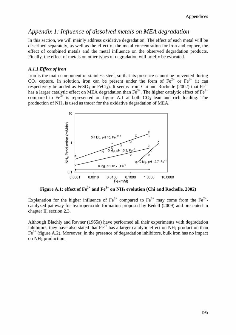
Appendices

195

Appendix 1: Influence of dissolved metals on MEA degradation

In this section, we will mainly address oxidative degradation. The effect of each metal will be

described separately, as well as the effect of the metal concentration for iron and copper, the

effect of combined metals and the metal influence on the observed degradation products.

Finally, the effect of metals on other types of degradation will briefly be evocated.

A.1.1 Effect of iron

Iron is the main component of stainless steel, so that its presence cannot be prevented during

CO2 capture. In solution, iron can be present under the form of Fe2+

or Fe3+

(it can

respectively be added as FeSO4 or FeCl3). It seems from Chi and Rochelle (2002) that Fe2+

has a larger catalytic effect on MEA degradation than Fe3+

. The higher catalytic effect of Fe2+

compared to Fe3+

is represented on figure A.1 at both CO2 lean and rich loading. The

production of NH3 is used as tracer for the oxidative degradation of MEA.

Figure A.1: effect of Fe2+

and Fe3+

on NH3 evolution (Chi and Rochelle, 2002)

Explanation for the higher influence of Fe2+

compared to Fe3+

may come from the Fe2+

-

catalyzed pathway for hydroperoxide formation proposed by Bedell (2009) and presented in

chapter II, section 2.3.

Although Blachly and Ravner (1965a) have performed all their experiments with degradation

inhibitors, they have also stated that Fe2+

has a larger catalytic effect on NH3 production than

Fe3+

(figure A.2). Moreover, in the presence of degradation inhibitors, bulk iron has no impact

on NH3 production.

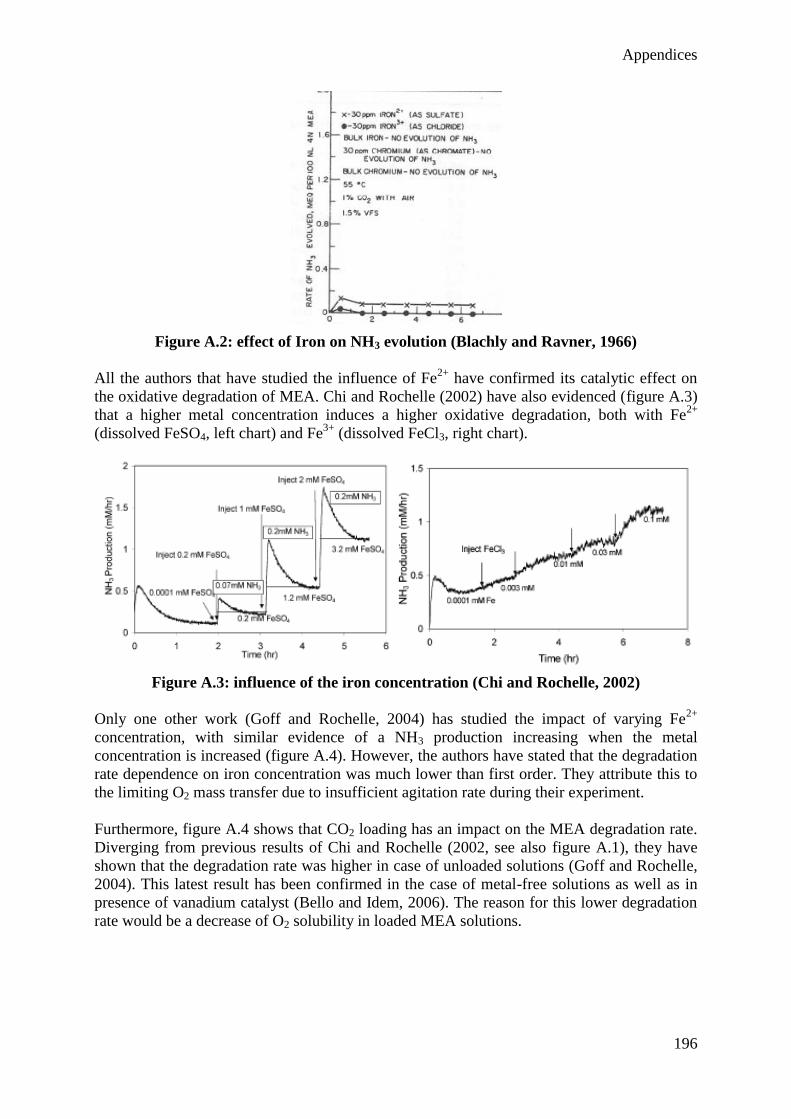
Appendices

196

Figure A.2: effect of Iron on NH3 evolution (Blachly and Ravner, 1966)

All the authors that have studied the influence of Fe2+

have confirmed its catalytic effect on

the oxidative degradation of MEA. Chi and Rochelle (2002) have also evidenced (figure A.3)

that a higher metal concentration induces a higher oxidative degradation, both with Fe2+

(dissolved FeSO4, left chart) and Fe3+

(dissolved FeCl3, right chart).

Figure A.3: influence of the iron concentration (Chi and Rochelle, 2002)

Only one other work (Goff and Rochelle, 2004) has studied the impact of varying Fe2+

concentration, with similar evidence of a NH3 production increasing when the metal

concentration is increased (figure A.4). However, the authors have stated that the degradation

rate dependence on iron concentration was much lower than first order. They attribute this to

the limiting O2 mass transfer due to insufficient agitation rate during their experiment.

Furthermore, figure A.4 shows that CO2 loading has an impact on the MEA degradation rate.

Diverging from previous results of Chi and Rochelle (2002, see also figure A.1), they have

shown that the degradation rate was higher in case of unloaded solutions (Goff and Rochelle,

2004). This latest result has been confirmed in the case of metal-free solutions as well as in

presence of vanadium catalyst (Bello and Idem, 2006). The reason for this lower degradation

rate would be a decrease of O2 solubility in loaded MEA solutions.

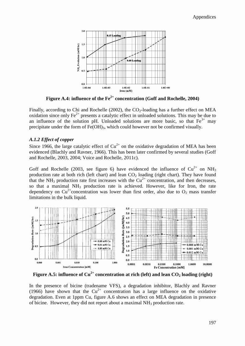
Appendices

197

Figure A.4: influence of the Fe2+

concentration (Goff and Rochelle, 2004)

Finally, according to Chi and Rochelle (2002), the CO2-loading has a further effect on MEA

oxidation since only Fe2+

presents a catalytic effect in unloaded solutions. This may be due to

an influence of the solution pH. Unloaded solutions are more basic, so that Fe3+

may

precipitate under the form of Fe(OH)3, which could however not be confirmed visually.

A.1.2 Effect of copper

Since 1966, the large catalytic effect of Cu2+

on the oxidative degradation of MEA has been

evidenced (Blachly and Ravner, 1966). This has been later confirmed by several studies (Goff

and Rochelle, 2003, 2004; Voice and Rochelle, 2011c).

Goff and Rochelle (2003, see figure 6) have evidenced the influence of Cu2+

on NH3

production rate at both rich (left chart) and lean CO2 loading (right chart). They have found

that the NH3 production rate first increases with the Cu2+

concentration, and then decreases,

so that a maximal NH3 production rate is achieved. However, like for Iron, the rate

dependency on Cu2+

concentration was lower than first order, also due to O2 mass transfer

limitations in the bulk liquid.

Figure A.5: influence of Cu2+

concentration at rich (left) and lean CO2 loading (right)

In the presence of bicine (tradename VFS), a degradation inhibitor, Blachly and Ravner

(1966) have shown that the Cu2+

concentration has a large influence on the oxidative

degradation. Even at 1ppm Cu, figure A.6 shows an effect on MEA degradation in presence

of bicine. However, they did not report about a maximal NH3 production rate.

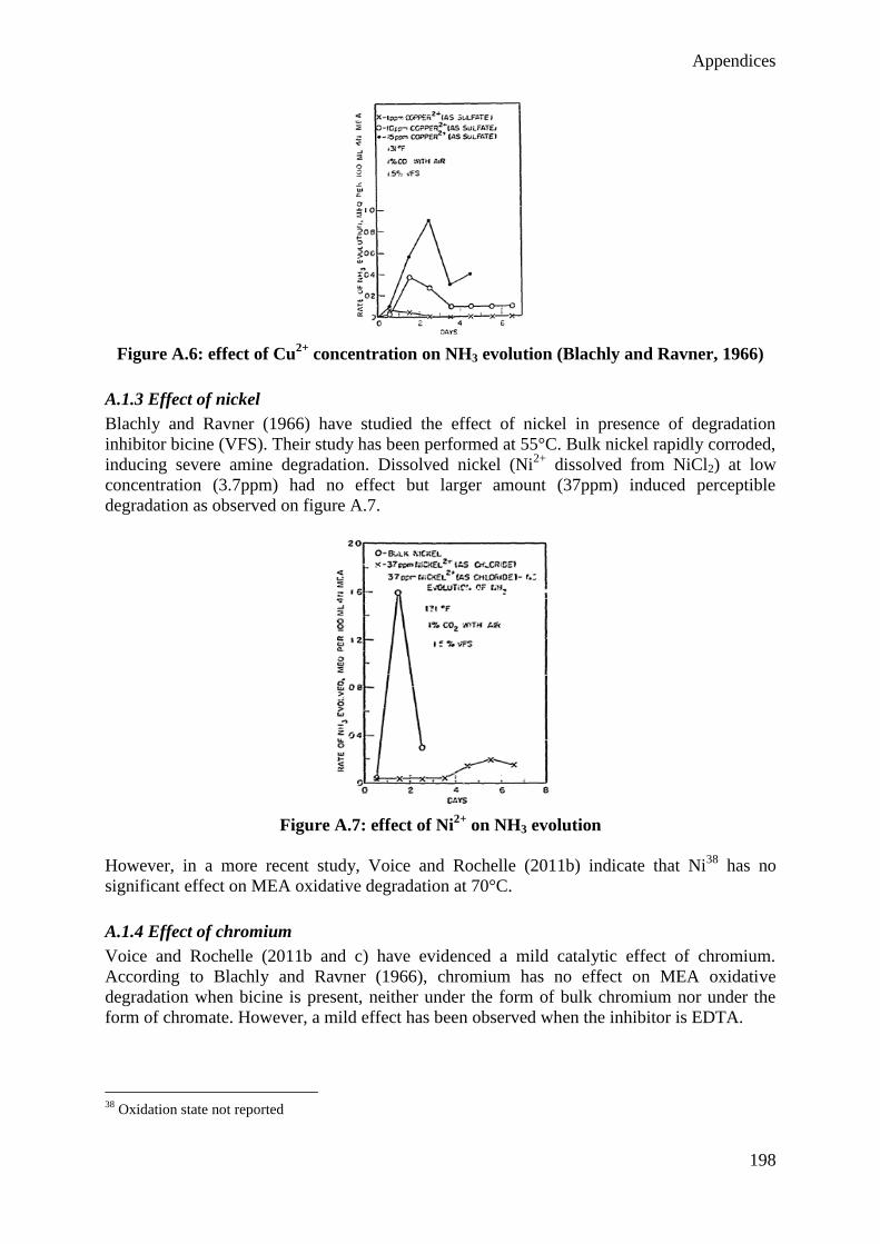
Appendices

198

Figure A.6: effect of Cu2+

concentration on NH3 evolution (Blachly and Ravner, 1966)

A.1.3 Effect of nickel

Blachly and Ravner (1966) have studied the effect of nickel in presence of degradation

inhibitor bicine (VFS). Their study has been performed at 55°C. Bulk nickel rapidly corroded,

inducing severe amine degradation. Dissolved nickel (Ni2+

dissolved from NiCl2) at low

concentration (3.7ppm) had no effect but larger amount (37ppm) induced perceptible

degradation as observed on figure A.7.

Figure A.7: effect of Ni2+

on NH3 evolution

However, in a more recent study, Voice and Rochelle (2011b) indicate that Ni38

has no

significant effect on MEA oxidative degradation at 70°C.

A.1.4 Effect of chromium

Voice and Rochelle (2011b and c) have evidenced a mild catalytic effect of chromium.

According to Blachly and Ravner (1966), chromium has no effect on MEA oxidative

degradation when bicine is present, neither under the form of bulk chromium nor under the

form of chromate. However, a mild effect has been observed when the inhibitor is EDTA.

38

Oxidation state not reported

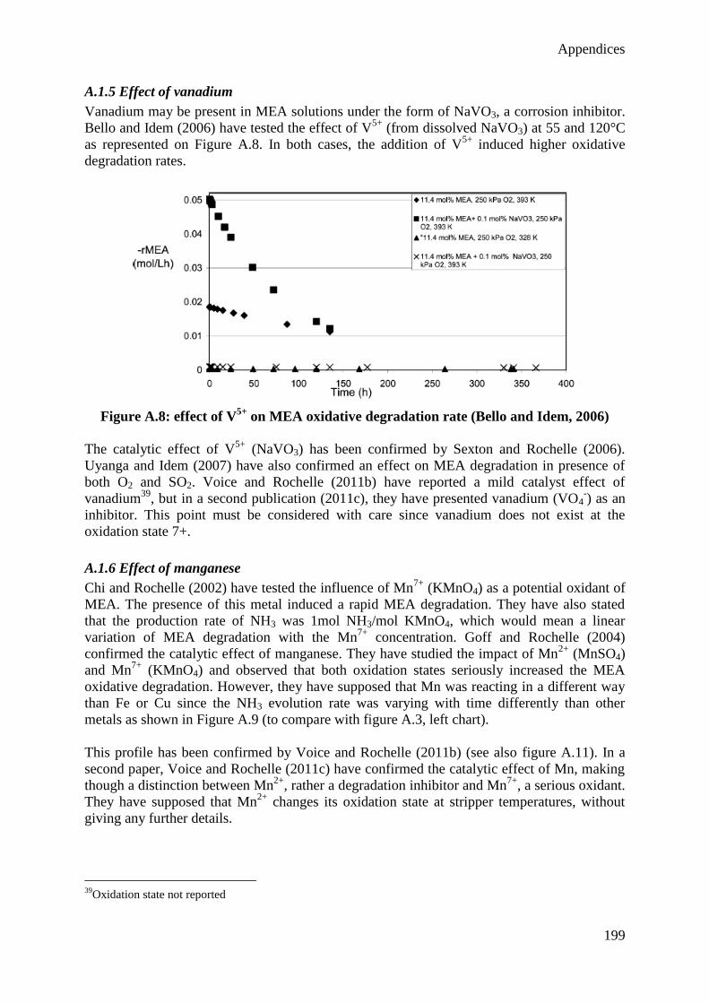
Appendices

199

A.1.5 Effect of vanadium

Vanadium may be present in MEA solutions under the form of NaVO3, a corrosion inhibitor.

Bello and Idem (2006) have tested the effect of V5+

(from dissolved NaVO3) at 55 and 120°C

as represented on Figure A.8. In both cases, the addition of V5+

induced higher oxidative

degradation rates.

Figure A.8: effect of V5+

on MEA oxidative degradation rate (Bello and Idem, 2006)

The catalytic effect of V5+

(NaVO3) has been confirmed by Sexton and Rochelle (2006).

Uyanga and Idem (2007) have also confirmed an effect on MEA degradation in presence of

both O2 and SO2. Voice and Rochelle (2011b) have reported a mild catalyst effect of

vanadium39

, but in a second publication (2011c), they have presented vanadium (VO4-) as an

inhibitor. This point must be considered with care since vanadium does not exist at the

oxidation state 7+.

A.1.6 Effect of manganese

Chi and Rochelle (2002) have tested the influence of Mn7+

(KMnO4) as a potential oxidant of

MEA. The presence of this metal induced a rapid MEA degradation. They have also stated

that the production rate of NH3 was 1mol NH3/mol KMnO4, which would mean a linear

variation of MEA degradation with the Mn7+

concentration. Goff and Rochelle (2004)

confirmed the catalytic effect of manganese. They have studied the impact of Mn2+

(MnSO4)

and Mn7+

(KMnO4) and observed that both oxidation states seriously increased the MEA

oxidative degradation. However, they have supposed that Mn was reacting in a different way

than Fe or Cu since the NH3 evolution rate was varying with time differently than other

metals as shown in Figure A.9 (to compare with figure A.3, left chart).

This profile has been confirmed by Voice and Rochelle (2011b) (see also figure A.11). In a

second paper, Voice and Rochelle (2011c) have confirmed the catalytic effect of Mn, making

though a distinction between Mn2+

, rather a degradation inhibitor and Mn7+

, a serious oxidant.

They have supposed that Mn2+

changes its oxidation state at stripper temperatures, without

giving any further details.

39

Oxidation state not reported

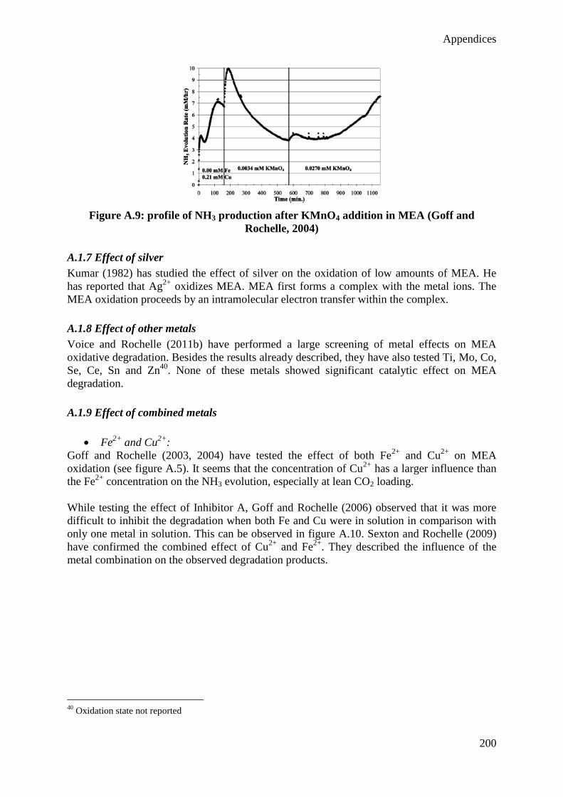
Appendices

200

Figure A.9: profile of NH3 production after KMnO4 addition in MEA (Goff and

Rochelle, 2004)

A.1.7 Effect of silver

Kumar (1982) has studied the effect of silver on the oxidation of low amounts of MEA. He

has reported that Ag2+

oxidizes MEA. MEA first forms a complex with the metal ions. The

MEA oxidation proceeds by an intramolecular electron transfer within the complex.

A.1.8 Effect of other metals

Voice and Rochelle (2011b) have performed a large screening of metal effects on MEA

oxidative degradation. Besides the results already described, they have also tested Ti, Mo, Co,

Se, Ce, Sn and Zn40

. None of these metals showed significant catalytic effect on MEA

degradation.

A.1.9 Effect of combined metals

Fe2+

and Cu2+

:

Goff and Rochelle (2003, 2004) have tested the effect of both Fe2+

and Cu2+

on MEA

oxidation (see figure A.5). It seems that the concentration of Cu2+

has a larger influence than

the Fe2+

concentration on the NH3 evolution, especially at lean CO2 loading.

While testing the effect of Inhibitor A, Goff and Rochelle (2006) observed that it was more

difficult to inhibit the degradation when both Fe and Cu were in solution in comparison with

only one metal in solution. This can be observed in figure A.10. Sexton and Rochelle (2009)

have confirmed the combined effect of Cu2+

and Fe2+

. They described the influence of the

metal combination on the observed degradation products.

40

Oxidation state not reported

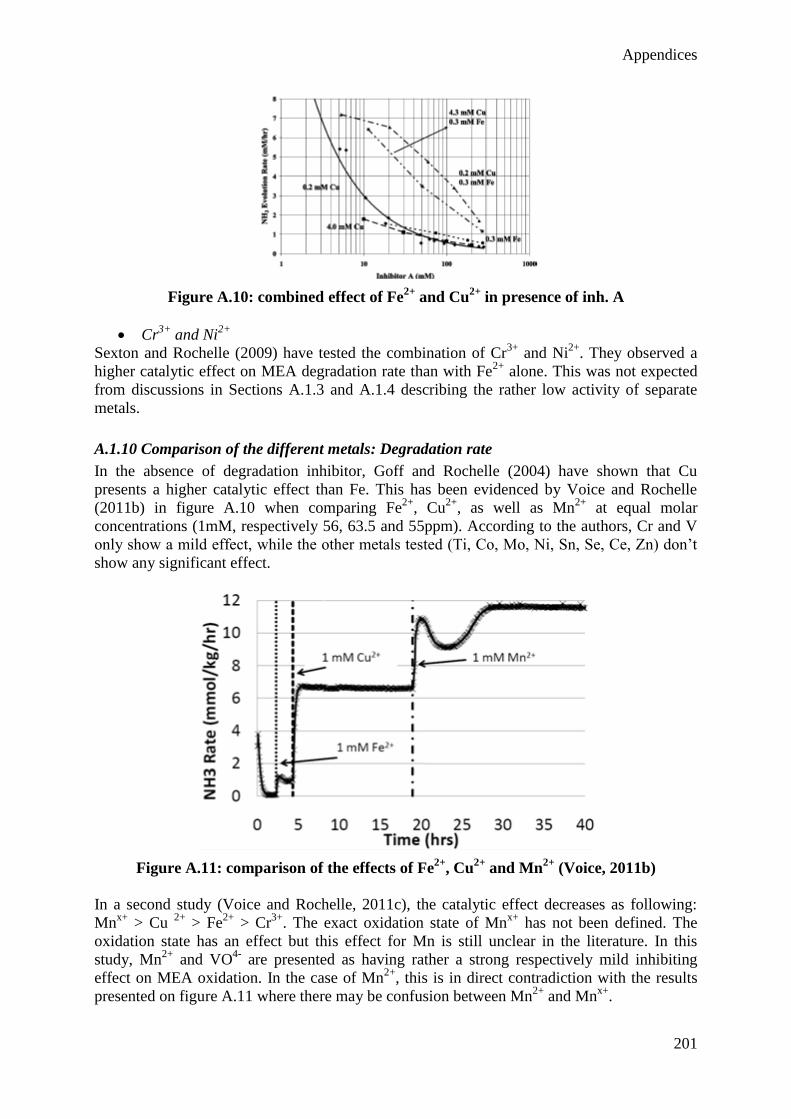
Appendices

201

Figure A.10: combined effect of Fe2+

and Cu2+

in presence of inh. A

Cr3+

and Ni2+

Sexton and Rochelle (2009) have tested the combination of Cr3+

and Ni2+

. They observed a

higher catalytic effect on MEA degradation rate than with Fe2+

alone. This was not expected

from discussions in Sections A.1.3 and A.1.4 describing the rather low activity of separate

metals.

A.1.10 Comparison of the different metals: Degradation rate

In the absence of degradation inhibitor, Goff and Rochelle (2004) have shown that Cu

presents a higher catalytic effect than Fe. This has been evidenced by Voice and Rochelle

(2011b) in figure A.10 when comparing Fe2+

, Cu2+

, as well as Mn2+

at equal molar

concentrations (1mM, respectively 56, 63.5 and 55ppm). According to the authors, Cr and V

only show a mild effect, while the other metals tested (Ti, Co, Mo, Ni, Sn, Se, Ce, Zn) don’t

show any significant effect.

Figure A.11: comparison of the effects of Fe2+

, Cu2+

and Mn2+

(Voice, 2011b)

In a second study (Voice and Rochelle, 2011c), the catalytic effect decreases as following:

Mnx+

> Cu 2+

> Fe2+

> Cr3+

. The exact oxidation state of Mnx+

has not been defined. The

oxidation state has an effect but this effect for Mn is still unclear in the literature. In this

study, Mn2+

and VO4-

are presented as having rather a strong respectively mild inhibiting

effect on MEA oxidation. In the case of Mn2+

, this is in direct contradiction with the results

presented on figure A.11 where there may be confusion between Mn2+

and Mnx+

.

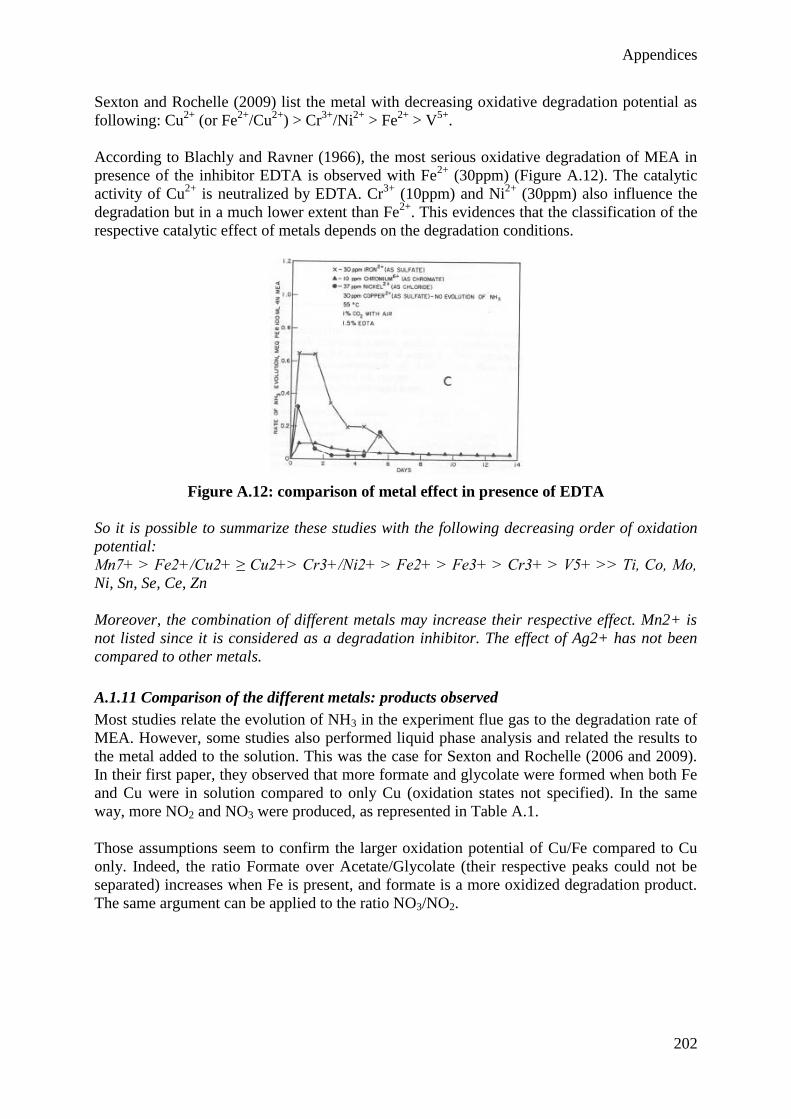
Appendices

202

Sexton and Rochelle (2009) list the metal with decreasing oxidative degradation potential as

following: Cu2+

(or Fe2+

/Cu2+

) > Cr3+

/Ni2+

> Fe2+

> V5+

.

According to Blachly and Ravner (1966), the most serious oxidative degradation of MEA in

presence of the inhibitor EDTA is observed with Fe2+

(30ppm) (Figure A.12). The catalytic

activity of Cu2+

is neutralized by EDTA. Cr3+

(10ppm) and Ni2+

(30ppm) also influence the

degradation but in a much lower extent than Fe2+

. This evidences that the classification of the

respective catalytic effect of metals depends on the degradation conditions.

Figure A.12: comparison of metal effect in presence of EDTA

So it is possible to summarize these studies with the following decreasing order of oxidation

potential:

Mn7+ > Fe2+/Cu2+ ≥ Cu2+> Cr3+/Ni2+ > Fe2+ > Fe3+ > Cr3+ > V5+ >> Ti, Co, Mo,

Ni, Sn, Se, Ce, Zn

Moreover, the combination of different metals may increase their respective effect. Mn2+ is

not listed since it is considered as a degradation inhibitor. The effect of Ag2+ has not been

compared to other metals.

A.1.11 Comparison of the different metals: products observed

Most studies relate the evolution of NH3 in the experiment flue gas to the degradation rate of

MEA. However, some studies also performed liquid phase analysis and related the results to

the metal added to the solution. This was the case for Sexton and Rochelle (2006 and 2009).

In their first paper, they observed that more formate and glycolate were formed when both Fe

and Cu were in solution compared to only Cu (oxidation states not specified). In the same

way, more NO2 and NO3 were produced, as represented in Table A.1.

Those assumptions seem to confirm the larger oxidation potential of Cu/Fe compared to Cu

only. Indeed, the ratio Formate over Acetate/Glycolate (their respective peaks could not be

separated) increases when Fe is present, and formate is a more oxidized degradation product.

The same argument can be applied to the ratio NO3/NO2.

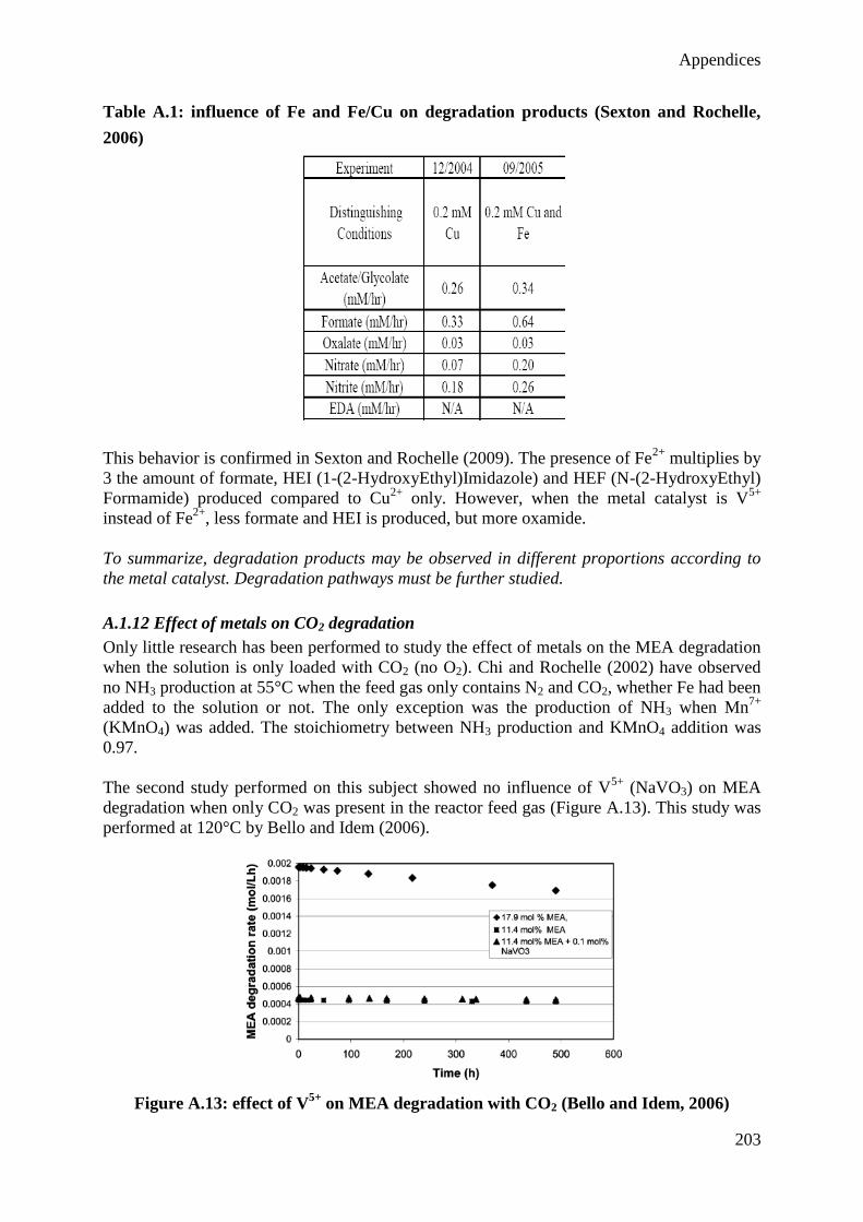
Appendices

203

Table A.1: influence of Fe and Fe/Cu on degradation products (Sexton and Rochelle,

2006)

This behavior is confirmed in Sexton and Rochelle (2009). The presence of Fe2+

multiplies by

3 the amount of formate, HEI (1-(2-HydroxyEthyl)Imidazole) and HEF (N-(2-HydroxyEthyl)

Formamide) produced compared to Cu2+

only. However, when the metal catalyst is V5+

instead of Fe2+

, less formate and HEI is produced, but more oxamide.

To summarize, degradation products may be observed in different proportions according to

the metal catalyst. Degradation pathways must be further studied.

A.1.12 Effect of metals on CO2 degradation

Only little research has been performed to study the effect of metals on the MEA degradation

when the solution is only loaded with CO2 (no O2). Chi and Rochelle (2002) have observed

no NH3 production at 55°C when the feed gas only contains N2 and CO2, whether Fe had been

added to the solution or not. The only exception was the production of NH3 when Mn7+

(KMnO4) was added. The stoichiometry between NH3 production and KMnO4 addition was

0.97.

The second study performed on this subject showed no influence of V5+

(NaVO3) on MEA

degradation when only CO2 was present in the reactor feed gas (Figure A.13). This study was

performed at 120°C by Bello and Idem (2006).

Figure A.13: effect of V5+

on MEA degradation with CO2 (Bello and Idem, 2006)

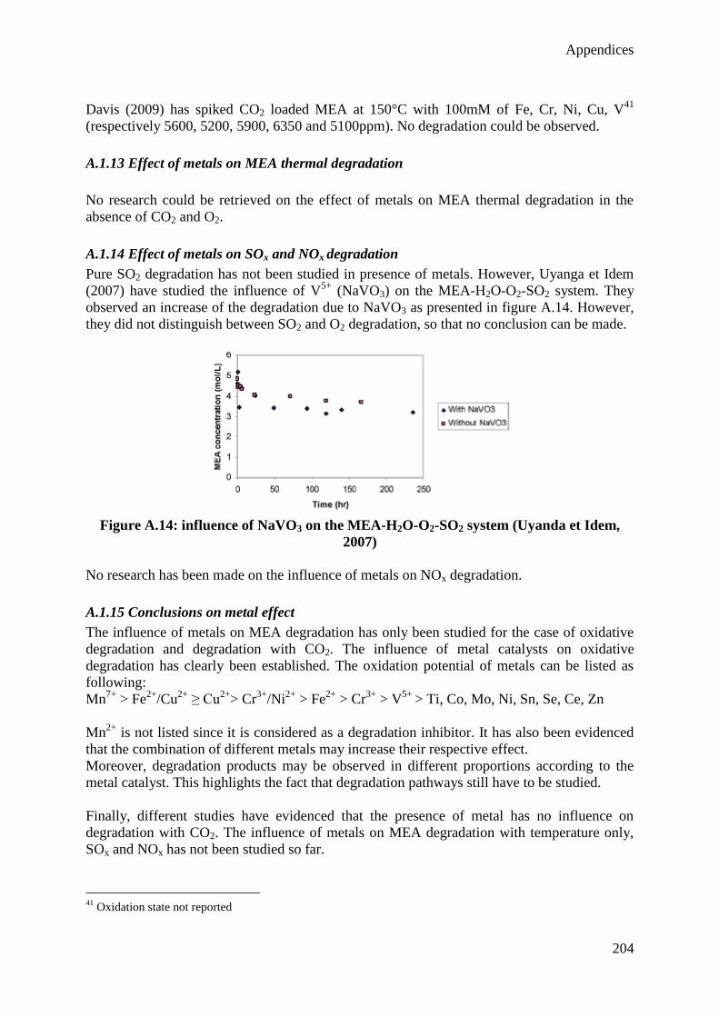
Appendices

204

Davis (2009) has spiked CO2 loaded MEA at 150°C with 100mM of Fe, Cr, Ni, Cu, V41

(respectively 5600, 5200, 5900, 6350 and 5100ppm). No degradation could be observed.

A.1.13 Effect of metals on MEA thermal degradation

No research could be retrieved on the effect of metals on MEA thermal degradation in the

absence of CO2 and O2.

A.1.14 Effect of metals on SOx and NOx degradation

Pure SO2 degradation has not been studied in presence of metals. However, Uyanga et Idem

(2007) have studied the influence of V5+

(NaVO3) on the MEA-H2O-O2-SO2 system. They

observed an increase of the degradation due to NaVO3 as presented in figure A.14. However,

they did not distinguish between SO2 and O2 degradation, so that no conclusion can be made.

Figure A.14: influence of NaVO3 on the MEA-H2O-O2-SO2 system (Uyanda et Idem,

2007)

No research has been made on the influence of metals on NOx degradation.

A.1.15 Conclusions on metal effect

The influence of metals on MEA degradation has only been studied for the case of oxidative

degradation and degradation with CO2. The influence of metal catalysts on oxidative

degradation has clearly been established. The oxidation potential of metals can be listed as

following:

Mn7+

> Fe2+

/Cu2+

≥ Cu2+

> Cr3+

/Ni2+

> Fe2+

> Cr3+

> V5+

> Ti, Co, Mo, Ni, Sn, Se, Ce, Zn

Mn2+

is not listed since it is considered as a degradation inhibitor. It has also been evidenced

that the combination of different metals may increase their respective effect.

Moreover, degradation products may be observed in different proportions according to the

metal catalyst. This highlights the fact that degradation pathways still have to be studied.

Finally, different studies have evidenced that the presence of metal has no influence on

degradation with CO2. The influence of metals on MEA degradation with temperature only,

SOx and NOx has not been studied so far.

41

Oxidation state not reported

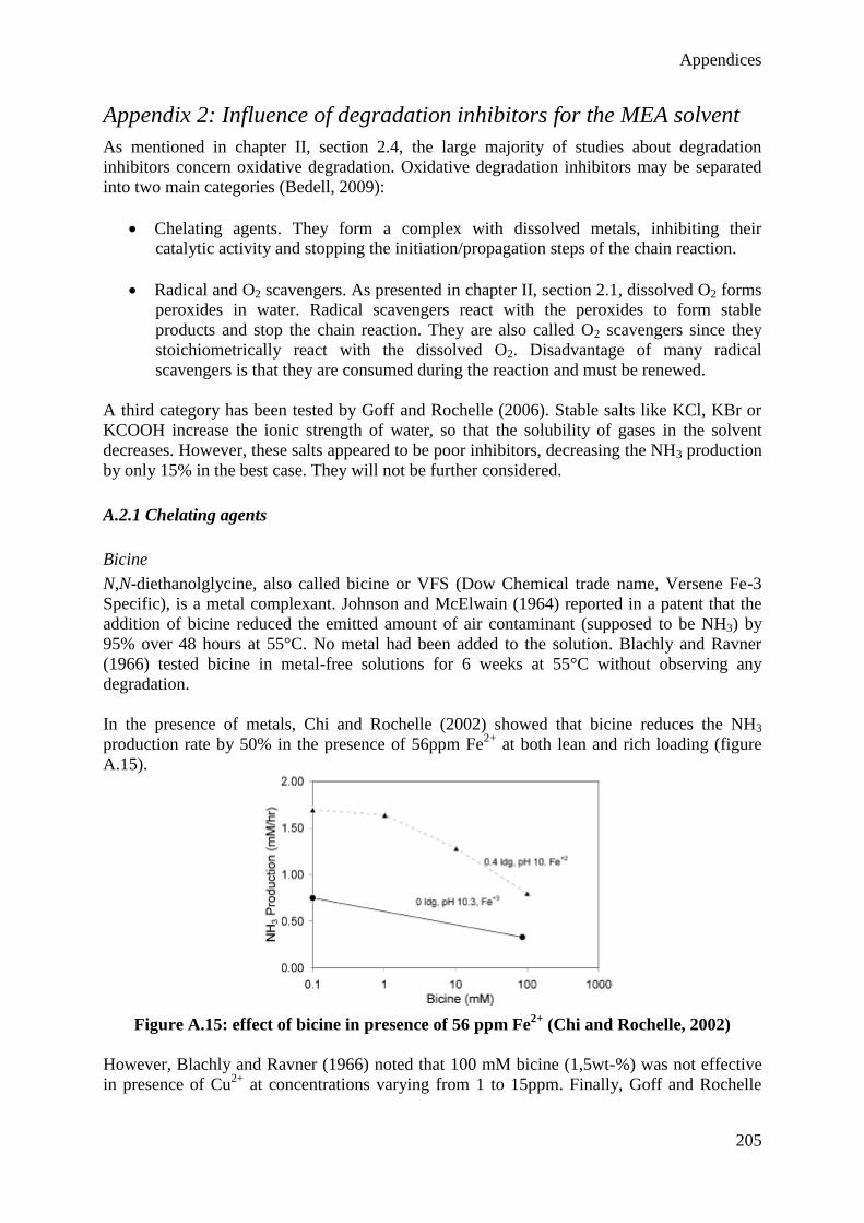
Appendices

205

Appendix 2: Influence of degradation inhibitors for the MEA solvent

As mentioned in chapter II, section 2.4, the large majority of studies about degradation

inhibitors concern oxidative degradation. Oxidative degradation inhibitors may be separated

into two main categories (Bedell, 2009):

Chelating agents. They form a complex with dissolved metals, inhibiting their

catalytic activity and stopping the initiation/propagation steps of the chain reaction.

Radical and O2 scavengers. As presented in chapter II, section 2.1, dissolved O2 forms

peroxides in water. Radical scavengers react with the peroxides to form stable

products and stop the chain reaction. They are also called O2 scavengers since they

stoichiometrically react with the dissolved O2. Disadvantage of many radical

scavengers is that they are consumed during the reaction and must be renewed.

A third category has been tested by Goff and Rochelle (2006). Stable salts like KCl, KBr or

KCOOH increase the ionic strength of water, so that the solubility of gases in the solvent

decreases. However, these salts appeared to be poor inhibitors, decreasing the NH3 production

by only 15% in the best case. They will not be further considered.

A.2.1 Chelating agents

Bicine

N,N-diethanolglycine, also called bicine or VFS (Dow Chemical trade name, Versene Fe-3

Specific), is a metal complexant. Johnson and McElwain (1964) reported in a patent that the

addition of bicine reduced the emitted amount of air contaminant (supposed to be NH3) by

95% over 48 hours at 55°C. No metal had been added to the solution. Blachly and Ravner

(1966) tested bicine in metal-free solutions for 6 weeks at 55°C without observing any

degradation.

In the presence of metals, Chi and Rochelle (2002) showed that bicine reduces the NH3

production rate by 50% in the presence of 56ppm Fe2+

at both lean and rich loading (figure

A.15).

Figure A.15: effect of bicine in presence of 56 ppm Fe2+

(Chi and Rochelle, 2002)

However, Blachly and Ravner (1966) noted that 100 mM bicine (1,5wt-%) was not effective

in presence of Cu2+

at concentrations varying from 1 to 15ppm. Finally, Goff and Rochelle

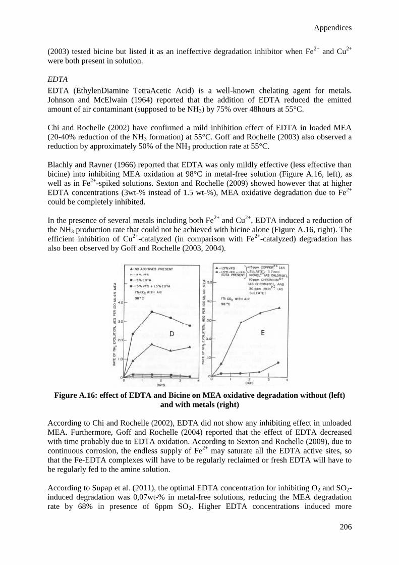
Appendices

206

(2003) tested bicine but listed it as an ineffective degradation inhibitor when Fe2+

and Cu2+

were both present in solution.

EDTA

EDTA (EthylenDiamine TetraAcetic Acid) is a well-known chelating agent for metals.

Johnson and McElwain (1964) reported that the addition of EDTA reduced the emitted

amount of air contaminant (supposed to be NH3) by 75% over 48hours at 55°C.

Chi and Rochelle (2002) have confirmed a mild inhibition effect of EDTA in loaded MEA

(20-40% reduction of the NH3 formation) at 55°C. Goff and Rochelle (2003) also observed a

reduction by approximately 50% of the NH3 production rate at 55°C.

Blachly and Ravner (1966) reported that EDTA was only mildly effective (less effective than

bicine) into inhibiting MEA oxidation at 98°C in metal-free solution (Figure A.16, left), as

well as in Fe2+

-spiked solutions. Sexton and Rochelle (2009) showed however that at higher

EDTA concentrations (3wt-% instead of 1.5 wt-%), MEA oxidative degradation due to Fe2+

could be completely inhibited.

In the presence of several metals including both Fe2+

and Cu2+

, EDTA induced a reduction of

the NH3 production rate that could not be achieved with bicine alone (Figure A.16, right). The

efficient inhibition of Cu2+

-catalyzed (in comparison with Fe2+

-catalyzed) degradation has

also been observed by Goff and Rochelle (2003, 2004).

Figure A.16: effect of EDTA and Bicine on MEA oxidative degradation without (left)

and with metals (right)

According to Chi and Rochelle (2002), EDTA did not show any inhibiting effect in unloaded

MEA. Furthermore, Goff and Rochelle (2004) reported that the effect of EDTA decreased

with time probably due to EDTA oxidation. According to Sexton and Rochelle (2009), due to

continuous corrosion, the endless supply of Fe2+

may saturate all the EDTA active sites, so

that the Fe-EDTA complexes will have to be regularly reclaimed or fresh EDTA will have to

be regularly fed to the amine solution.

According to Supap et al. (2011), the optimal EDTA concentration for inhibiting O2 and SO2-

induced degradation was 0,07wt-% in metal-free solutions, reducing the MEA degradation

rate by 68% in presence of 6ppm SO2. Higher EDTA concentrations induced more

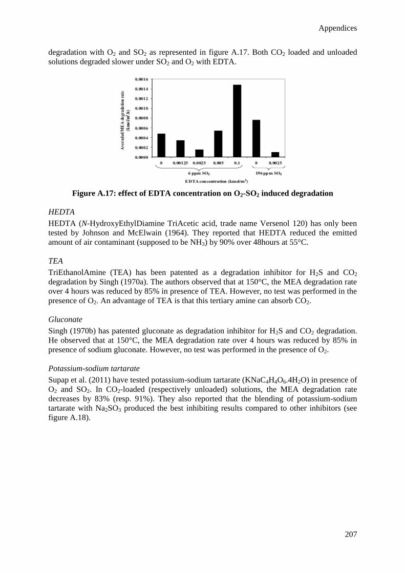
Appendices

207

degradation with O2 and SO2 as represented in figure A.17. Both CO2 loaded and unloaded

solutions degraded slower under SO2 and O2 with EDTA.

Figure A.17: effect of EDTA concentration on O2-SO2 induced degradation

HEDTA

HEDTA (N-HydroxyEthylDiamine TriAcetic acid, trade name Versenol 120) has only been

tested by Johnson and McElwain (1964). They reported that HEDTA reduced the emitted

amount of air contaminant (supposed to be NH3) by 90% over 48hours at 55°C.

TEA

TriEthanolAmine (TEA) has been patented as a degradation inhibitor for H2S and CO2

degradation by Singh (1970a). The authors observed that at 150°C, the MEA degradation rate

over 4 hours was reduced by 85% in presence of TEA. However, no test was performed in the

presence of O2. An advantage of TEA is that this tertiary amine can absorb CO2.

Gluconate

Singh (1970b) has patented gluconate as degradation inhibitor for H2S and CO2 degradation.

He observed that at 150°C, the MEA degradation rate over 4 hours was reduced by 85% in

presence of sodium gluconate. However, no test was performed in the presence of O2.

Potassium-sodium tartarate

Supap et al. (2011) have tested potassium-sodium tartarate (KNaC4H4O6.4H2O) in presence of

O2 and SO2. In CO2-loaded (respectively unloaded) solutions, the MEA degradation rate

decreases by 83% (resp. 91%). They also reported that the blending of potassium-sodium

tartarate with Na2SO3 produced the best inhibiting results compared to other inhibitors (see

figure A.18).

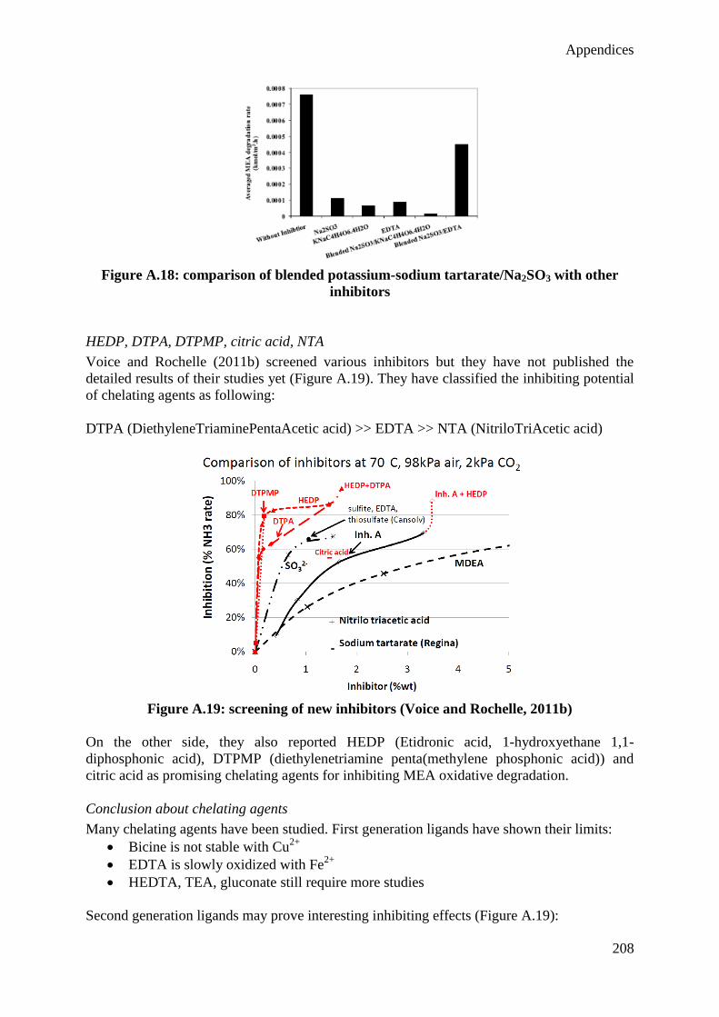
Appendices

208

Figure A.18: comparison of blended potassium-sodium tartarate/Na2SO3 with other

inhibitors

HEDP, DTPA, DTPMP, citric acid, NTA

Voice and Rochelle (2011b) screened various inhibitors but they have not published the

detailed results of their studies yet (Figure A.19). They have classified the inhibiting potential

of chelating agents as following:

DTPA (DiethyleneTriaminePentaAcetic acid) >> EDTA >> NTA (NitriloTriAcetic acid)

Figure A.19: screening of new inhibitors (Voice and Rochelle, 2011b)

On the other side, they also reported HEDP (Etidronic acid, 1-hydroxyethane 1,1-

diphosphonic acid), DTPMP (diethylenetriamine penta(methylene phosphonic acid)) and

citric acid as promising chelating agents for inhibiting MEA oxidative degradation.

Conclusion about chelating agents

Many chelating agents have been studied. First generation ligands have shown their limits:

Bicine is not stable with Cu2+

EDTA is slowly oxidized with Fe2+

HEDTA, TEA, gluconate still require more studies

Second generation ligands may prove interesting inhibiting effects (Figure A.19):

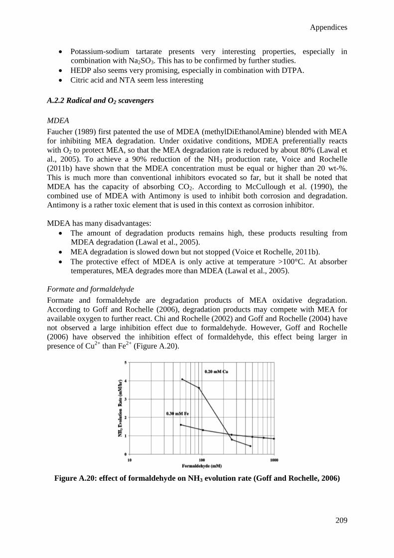
Appendices

209

Potassium-sodium tartarate presents very interesting properties, especially in

combination with Na2SO3. This has to be confirmed by further studies.

HEDP also seems very promising, especially in combination with DTPA.

Citric acid and NTA seem less interesting

A.2.2 Radical and O2 scavengers

MDEA

Faucher (1989) first patented the use of MDEA (methylDiEthanolAmine) blended with MEA

for inhibiting MEA degradation. Under oxidative conditions, MDEA preferentially reacts

with O2 to protect MEA, so that the MEA degradation rate is reduced by about 80% (Lawal et

al., 2005). To achieve a 90% reduction of the NH3 production rate, Voice and Rochelle

(2011b) have shown that the MDEA concentration must be equal or higher than 20 wt-%.

This is much more than conventional inhibitors evocated so far, but it shall be noted that

MDEA has the capacity of absorbing CO2. According to McCullough et al. (1990), the

combined use of MDEA with Antimony is used to inhibit both corrosion and degradation.

Antimony is a rather toxic element that is used in this context as corrosion inhibitor.

MDEA has many disadvantages:

The amount of degradation products remains high, these products resulting from

MDEA degradation (Lawal et al., 2005).

MEA degradation is slowed down but not stopped (Voice et Rochelle, 2011b).

The protective effect of MDEA is only active at temperature >100°C. At absorber

temperatures, MEA degrades more than MDEA (Lawal et al., 2005).

Formate and formaldehyde

Formate and formaldehyde are degradation products of MEA oxidative degradation.

According to Goff and Rochelle (2006), degradation products may compete with MEA for

available oxygen to further react. Chi and Rochelle (2002) and Goff and Rochelle (2004) have

not observed a large inhibition effect due to formaldehyde. However, Goff and Rochelle

(2006) have observed the inhibition effect of formaldehyde, this effect being larger in

presence of Cu2+

than Fe2+

(Figure A.20).

Figure A.20: effect of formaldehyde on NH3 evolution rate (Goff and Rochelle, 2006)

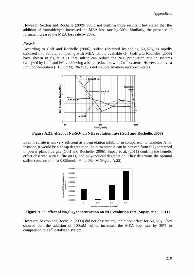
Appendices

210

However, Sexton and Rochelle (2009) could not confirm those results. They stated that the

addition of formaldehyde increased the MEA loss rate by 30%. Similarly, the presence of

formate increased the MEA loss rate by 20%.

Na2SO3

According to Goff and Rochelle (2006), sulfite (obtained by adding Na2SO3) is rapidly

oxidized into sulfate, competing with MEA for the available O2. Goff and Rochelle (2006)

have shown in figure A.21 that sulfite can reduce the NH3 production rate in systems

catalyzed by Cu2+

and Fe2+

, achieving a better reduction with Cu2+

systems. However, above a

limit concentration (~1000mM), Na2SO3 is not soluble anymore and precipitates.

Figure A.21: effect of Na2SO3 on NH3 evolution rate (Goff and Rochelle, 2006)

Even if sulfite is not very efficient as a degradation inhibitor in comparison to inhibitor A for

instance, it would be a cheap degradation inhibitor since it can be derived from SO2 contained

in power plant flue gas (Goff and Rochelle, 2006). Supap et al. (2011) confirm the benefic

effect observed with sulfite on O2 and SO2-induced degradation. They determine the optimal

sulfite concentration at 0.05kmol/m³, i.e. 50mM (Figure A.22).

Figure A.22: effect of Na2SO3 concentration on NH3 evolution rate (Supap et al., 2011)

However, Sexton and Rochelle (2009) did not observe any inhibition effect for Na2SO3. They

showed that the addition of 100mM sulfite increased the MEA loss rate by 30% in

comparison to Fe2+

-catalyzed system.

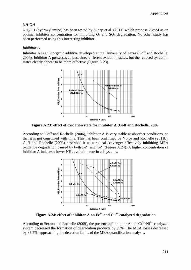
Appendices

211

NH2OH

NH2OH (hydroxylamine) has been tested by Supap et al. (2011) which propose 25mM as an

optimal inhibitor concentration for inhibiting O2 and SO2 degradation. No other study has

been performed using this interesting inhibitor.

Inhibitor A

Inhibitor A is an inorganic additive developed at the University of Texas (Goff and Rochelle,

2006). Inhibitor A possesses at least three different oxidation states, but the reduced oxidation

states clearly appear to be more effective (Figure A.23).

Figure A.23: effect of oxidation state for inhibitor A (Goff and Rochelle, 2006)

According to Goff and Rochelle (2006), inhibitor A is very stable at absorber conditions, so

that it is not consumed with time. This has been confirmed by Voice and Rochelle (2011b).

Goff and Rochelle (2006) described it as a radical scavenger effectively inhibiting MEA

oxidative degradation caused by both Fe2+

and Cu2+

(Figure A.24). A higher concentration of

inhibitor A induces a lower NH3 evolution rate in all systems.

Figure A.24: effect of inhibitor A on Fe2+

and Cu2+

catalyzed degradation

According to Sexton and Rochelle (2009), the presence of inhibitor A in a Cr3+

/Ni2+

-catalyzed

system decreased the formation of degradation products by 99%. The MEA losses decreased

by 87.5%, approaching the detection limits of the MEA quantification analysis.

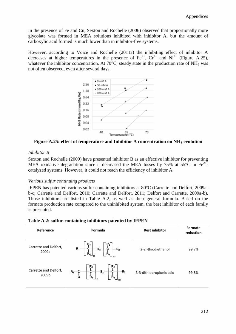
Appendices

212

In the presence of Fe and Cu, Sexton and Rochelle (2006) observed that proportionally more

glycolate was formed in MEA solutions inhibited with inhibitor A, but the amount of

carboxylic acid formed is much lower than in inhibitor-free systems.

However, according to Voice and Rochelle (2011a) the inhibiting effect of inhibitor A

decreases at higher temperatures in the presence of Fe2+

, Cr3+

and Ni2+

(Figure A.25),

whatever the inhibitor concentration. At 70°C, steady state in the production rate of NH3 was

not often observed, even after several days.

Figure A.25: effect of temperature and Inhibitor A concentration on NH3 evolution

Inhibitor B

Sexton and Rochelle (2009) have presented inhibitor B as an effective inhibitor for preventing

MEA oxidative degradation since it decreased the MEA losses by 75% at 55°C in Fe2+

-

catalyzed systems. However, it could not reach the efficiency of inhibitor A.

Various sulfur continuing products

IFPEN has patented various sulfur containing inhibitors at 80°C (Carrette and Delfort, 2009a-

b-c; Carrette and Delfort, 2010; Carrette and Delfort, 2011; Delfort and Carrette, 2009a-b).

Those inhibitors are listed in Table A.2, as well as their general formula. Based on the

formate production rate compared to the uninhibited system, the best inhibitor of each family

is presented.

Table A.2: sulfur-containing inhibitors patented by IFPEN

Reference Formula Best inhibitor Formate

reduction

Carrette and Delfort, 2009a

2-2’-thiodiethanol 99,7%

Carrette and Delfort, 2009b

3-3-dithiopropionic acid 99,8%

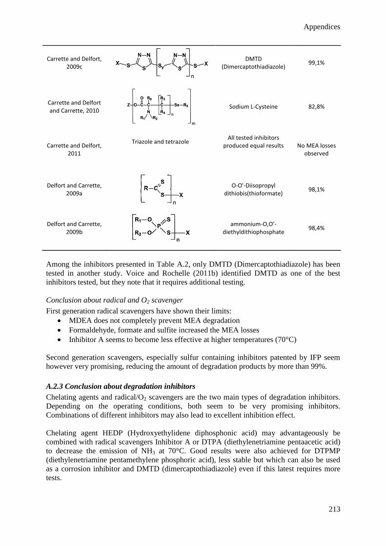
Appendices

213

Carrette and Delfort, 2009c

DMTD (Dimercaptothiadiazole)

99,1%

Carrette and Delfort and Carrette, 2010

Sodium L-Cysteine 82,8%

Carrette and Delfort, 2011

Triazole and tetrazole

All tested inhibitors produced equal results

No MEA losses observed

Delfort and Carrette, 2009a

O-O'-Diisopropyl dithiobis(thioformate)

98,1%

Delfort and Carrette, 2009b

ammonium-O,O’-diethyldithiophosphate

98,4%

Among the inhibitors presented in Table A.2, only DMTD (Dimercaptothiadiazole) has been

tested in another study. Voice and Rochelle (2011b) identified DMTD as one of the best

inhibitors tested, but they note that it requires additional testing.

Conclusion about radical and O2 scavenger

First generation radical scavengers have shown their limits:

MDEA does not completely prevent MEA degradation

Formaldehyde, formate and sulfite increased the MEA losses

Inhibitor A seems to become less effective at higher temperatures (70°C)

Second generation scavengers, especially sulfur containing inhibitors patented by IFP seem

however very promising, reducing the amount of degradation products by more than 99%.

A.2.3 Conclusion about degradation inhibitors

Chelating agents and radical/O2 scavengers are the two main types of degradation inhibitors.

Depending on the operating conditions, both seem to be very promising inhibitors.

Combinations of different inhibitors may also lead to excellent inhibition effect.

Chelating agent HEDP (Hydroxyethylidene diphosphonic acid) may advantageously be

combined with radical scavengers Inhibitor A or DTPA (diethylenetriamine pentaacetic acid)

to decrease the emission of NH3 at 70°C. Good results were also achieved for DTPMP

(diethylenetriamine pentamethylene phosphoric acid), less stable but which can also be used

as a corrosion inhibitor and DMTD (dimercaptothiadiazole) even if this latest requires more

tests.

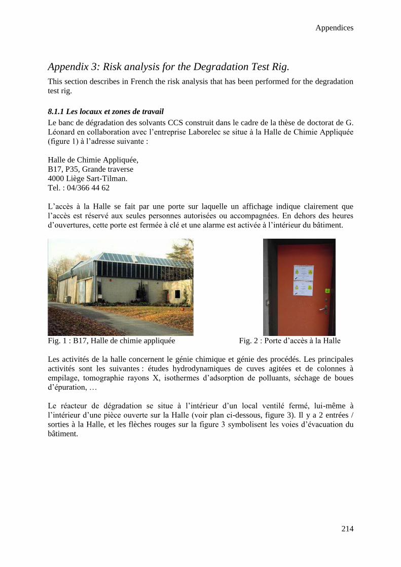
Appendices

214

Appendix 3: Risk analysis for the Degradation Test Rig.

This section describes in French the risk analysis that has been performed for the degradation

test rig.

8.1.1 Les locaux et zones de travail

Le banc de dégradation des solvants CCS construit dans le cadre de la thèse de doctorat de G.

Léonard en collaboration avec l’entreprise Laborelec se situe à la Halle de Chimie Appliquée

(figure 1) à l’adresse suivante :

Halle de Chimie Appliquée,

B17, P35, Grande traverse

4000 Liège Sart-Tilman.

Tel. : 04/366 44 62

L’accès à la Halle se fait par une porte sur laquelle un affichage indique clairement que

l’accès est réservé aux seules personnes autorisées ou accompagnées. En dehors des heures

d’ouvertures, cette porte est fermée à clé et une alarme est activée à l’intérieur du bâtiment.

Fig. 1 : B17, Halle de chimie appliquée Fig. 2 : Porte d’accès à la Halle

Les activités de la halle concernent le génie chimique et génie des procédés. Les principales

activités sont les suivantes : études hydrodynamiques de cuves agitées et de colonnes à

empilage, tomographie rayons X, isothermes d’adsorption de polluants, séchage de boues

d’épuration, …

Le réacteur de dégradation se situe à l’intérieur d’un local ventilé fermé, lui-même à

l’intérieur d’une pièce ouverte sur la Halle (voir plan ci-dessous, figure 3). Il y a 2 entrées /

sorties à la Halle, et les flèches rouges sur la figure 3 symbolisent les voies d’évacuation du

bâtiment.

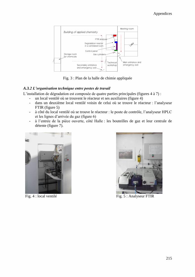
Appendices

215

Main entrance andemergency exit

Degradation reactorin a ventilated room

Building of applied chemistry

Labs

FTIR analyser

Control panel

TechnicalworkshopSecondary entrance

and emergency exit

Gas cylinders

Meeting room

Storage roomfor chemicals

Fig. 3 : Plan de la halle de chimie appliquée

A.3.2 L’organisation technique entre postes de travail

L’installation de dégradation est composée de quatre parties principales (figures 4 à 7) :

- un local ventilé où se trouvent le réacteur et ses auxiliaires (figure 4)

- dans un deuxième local ventilé voisin de celui où se trouve le réacteur : l’analyseur

FTIR (figure 5)

- à côté du local ventilé où se trouve le réacteur : le poste de contrôle, l’analyseur HPLC

et les lignes d’arrivée du gaz (figure 6)

- à l’entrée de la pièce ouverte, côté Halle : les bouteilles de gaz et leur centrale de

détente (figure 7).

Fig. 4 : local ventilé Fig. 5 : Analyseur FTIR

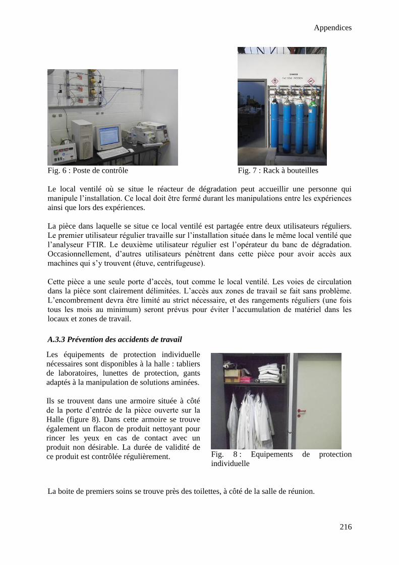
Appendices

216

Fig. 6 : Poste de contrôle Fig. 7 : Rack à bouteilles

Le local ventilé où se situe le réacteur de dégradation peut accueillir une personne qui

manipule l’installation. Ce local doit être fermé durant les manipulations entre les expériences

ainsi que lors des expériences.

La pièce dans laquelle se situe ce local ventilé est partagée entre deux utilisateurs réguliers.

Le premier utilisateur régulier travaille sur l’installation située dans le même local ventilé que

l’analyseur FTIR. Le deuxième utilisateur régulier est l’opérateur du banc de dégradation.

Occasionnellement, d’autres utilisateurs pénètrent dans cette pièce pour avoir accès aux

machines qui s’y trouvent (étuve, centrifugeuse).

Cette pièce a une seule porte d’accès, tout comme le local ventilé. Les voies de circulation

dans la pièce sont clairement délimitées. L’accès aux zones de travail se fait sans problème.

L’encombrement devra être limité au strict nécessaire, et des rangements réguliers (une fois

tous les mois au minimum) seront prévus pour éviter l’accumulation de matériel dans les

locaux et zones de travail.

A.3.3 Prévention des accidents de travail

Fig. 8 : Equipements de protection

individuelle

La boite de premiers soins se trouve près des toilettes, à côté de la salle de réunion.

Les équipements de protection individuelle

nécessaires sont disponibles à la halle : tabliers

de laboratoires, lunettes de protection, gants

adaptés à la manipulation de solutions aminées.

Ils se trouvent dans une armoire située à côté

de la porte d’entrée de la pièce ouverte sur la

Halle (figure 8). Dans cette armoire se trouve

également un flacon de produit nettoyant pour

rincer les yeux en cas de contact avec un

produit non désirable. La durée de validité de

ce produit est contrôlée régulièrement.

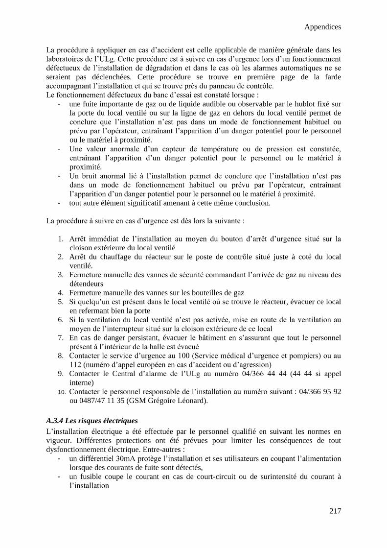
Appendices

217

La procédure à appliquer en cas d’accident est celle applicable de manière générale dans les

laboratoires de l’ULg. Cette procédure est à suivre en cas d’urgence lors d’un fonctionnement

défectueux de l’installation de dégradation et dans le cas où les alarmes automatiques ne se

seraient pas déclenchées. Cette procédure se trouve en première page de la farde

accompagnant l’installation et qui se trouve près du panneau de contrôle.

Le fonctionnement défectueux du banc d’essai est constaté lorsque :

- une fuite importante de gaz ou de liquide audible ou observable par le hublot fixé sur

la porte du local ventilé ou sur la ligne de gaz en dehors du local ventilé permet de

conclure que l’installation n’est pas dans un mode de fonctionnement habituel ou

prévu par l’opérateur, entraînant l’apparition d’un danger potentiel pour le personnel

ou le matériel à proximité.

- Une valeur anormale d’un capteur de température ou de pression est constatée,

entraînant l’apparition d’un danger potentiel pour le personnel ou le matériel à

proximité.

- Un bruit anormal lié à l’installation permet de conclure que l’installation n’est pas

dans un mode de fonctionnement habituel ou prévu par l’opérateur, entraînant

l’apparition d’un danger potentiel pour le personnel ou le matériel à proximité.

- tout autre élément significatif amenant à cette même conclusion.

La procédure à suivre en cas d’urgence est dès lors la suivante :

1. Arrêt immédiat de l’installation au moyen du bouton d’arrêt d’urgence situé sur la

cloison extérieure du local ventilé

2. Arrêt du chauffage du réacteur sur le poste de contrôle situé juste à coté du local

ventilé.

3. Fermeture manuelle des vannes de sécurité commandant l’arrivée de gaz au niveau des

détendeurs

4. Fermeture manuelle des vannes sur les bouteilles de gaz

5. Si quelqu’un est présent dans le local ventilé où se trouve le réacteur, évacuer ce local

en refermant bien la porte

6. Si la ventilation du local ventilé n’est pas activée, mise en route de la ventilation au

moyen de l’interrupteur situé sur la cloison extérieure de ce local

7. En cas de danger persistant, évacuer le bâtiment en s’assurant que tout le personnel

présent à l’intérieur de la halle est évacué

8. Contacter le service d’urgence au 100 (Service médical d’urgence et pompiers) ou au

112 (numéro d’appel européen en cas d’accident ou d’agression)

9. Contacter le Central d’alarme de l’ULg au numéro 04/366 44 44 (44 44 si appel

interne)

10. Contacter le personnel responsable de l’installation au numéro suivant : 04/366 95 92

ou 0487/47 11 35 (GSM Grégoire Léonard).

A.3.4 Les risques électriques

L’installation électrique a été effectuée par le personnel qualifié en suivant les normes en

vigueur. Différentes protections ont été prévues pour limiter les conséquences de tout

dysfonctionnement électrique. Entre-autres :

- un différentiel 30mA protège l’installation et ses utilisateurs en coupant l’alimentation

lorsque des courants de fuite sont détectés,

- un fusible coupe le courant en cas de court-circuit ou de surintensité du courant à

l’installation

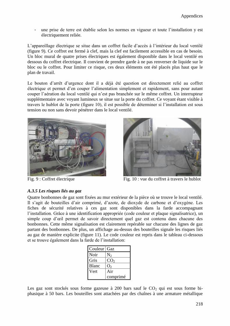
Appendices

218

- une prise de terre est établie selon les normes en vigueur et toute l’installation y est

électriquement reliée.

L’appareillage électrique se situe dans un coffret facile d’accès à l’intérieur du local ventilé

(figure 9). Ce coffret est fermé à clef, mais la clef est facilement accessible en cas de besoin.

Un bloc mural de quatre prises électriques est également disponible dans le local ventilé en

dessous du coffret électrique. Il convient de prendre garde à ne pas renverser de liquide sur le

bloc ou le coffret. Pour limiter ce risque, ces deux éléments ont été placés plus haut que le

plan de travail.

Le bouton d’arrêt d’urgence dont il a déjà été question est directement relié au coffret

électrique et permet d’en couper l’alimentation simplement et rapidement, sans pour autant

couper l’aération du local ventilé qui n’est pas branchée sur le même coffret. Un interrupteur

supplémentaire avec voyant lumineux se situe sur la porte du coffret. Ce voyant étant visible à

travers le hublot de la porte (figure 10), il est possible de déterminer si l’installation est sous

tension ou non sans devoir pénétrer dans le local ventilé.

Fig. 9 : Coffret électrique Fig. 10 : vue du coffret à travers le hublot

A.3.5 Les risques liés au gaz

Quatre bonbonnes de gaz sont fixées au mur extérieur de la pièce où se trouve le local ventilé.

Il s’agit de bouteilles d’air comprimé, d’azote, de dioxyde de carbone et d’oxygène. Les

fiches de sécurité relatives à ces gaz sont disponibles dans la farde accompagnant

l’installation. Grâce à une identification appropriée (code couleur et plaque signalisatrice), un

simple coup d’œil permet de savoir directement quel gaz est contenu dans chacune des

bonbonnes. Cette même signalisation est clairement repérable sur chacune des lignes de gaz

partant des bonbonnes. De plus, un affichage au-dessus des bouteilles signale les risques liés

au gaz de manière explicite (figure 11). Le code couleur est repris dans le tableau ci-dessous

et se trouve également dans la farde de l’installation:

Les gaz sont stockés sous forme gazeuse à 200 bars sauf le CO2 qui est sous forme bi-

phasique à 50 bars. Les bouteilles sont attachées par des chaînes à une armature métallique

Couleur Gaz

Noir N2

Gris CO2

Blanc O2

Vert Air

comprimé

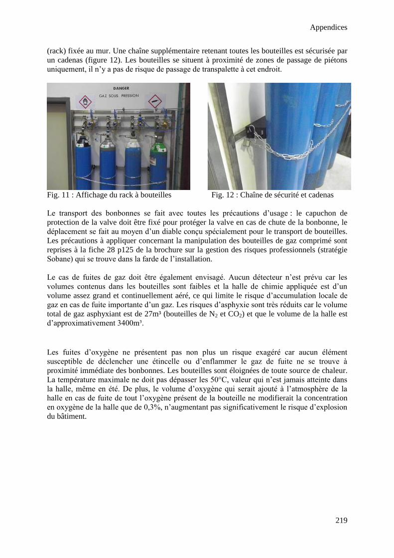
Appendices

219

(rack) fixée au mur. Une chaîne supplémentaire retenant toutes les bouteilles est sécurisée par

un cadenas (figure 12). Les bouteilles se situent à proximité de zones de passage de piétons

uniquement, il n’y a pas de risque de passage de transpalette à cet endroit.

Fig. 11 : Affichage du rack à bouteilles Fig. 12 : Chaîne de sécurité et cadenas

Le transport des bonbonnes se fait avec toutes les précautions d’usage : le capuchon de

protection de la valve doit être fixé pour protéger la valve en cas de chute de la bonbonne, le

déplacement se fait au moyen d’un diable conçu spécialement pour le transport de bouteilles.

Les précautions à appliquer concernant la manipulation des bouteilles de gaz comprimé sont

reprises à la fiche 28 p125 de la brochure sur la gestion des risques professionnels (stratégie

Sobane) qui se trouve dans la farde de l’installation.

Le cas de fuites de gaz doit être également envisagé. Aucun détecteur n’est prévu car les

volumes contenus dans les bouteilles sont faibles et la halle de chimie appliquée est d’un

volume assez grand et continuellement aéré, ce qui limite le risque d’accumulation locale de

gaz en cas de fuite importante d’un gaz. Les risques d’asphyxie sont très réduits car le volume

total de gaz asphyxiant est de 27m³ (bouteilles de N2 et CO2) et que le volume de la halle est

d’approximativement 3400m³.

Les fuites d’oxygène ne présentent pas non plus un risque exagéré car aucun élément

susceptible de déclencher une étincelle ou d’enflammer le gaz de fuite ne se trouve à

proximité immédiate des bonbonnes. Les bouteilles sont éloignées de toute source de chaleur.

La température maximale ne doit pas dépasser les 50°C, valeur qui n’est jamais atteinte dans

la halle, même en été. De plus, le volume d’oxygène qui serait ajouté à l’atmosphère de la

halle en cas de fuite de tout l’oxygène présent de la bouteille ne modifierait la concentration

en oxygène de la halle que de 0,3%, n’augmentant pas significativement le risque d’explosion

du bâtiment.

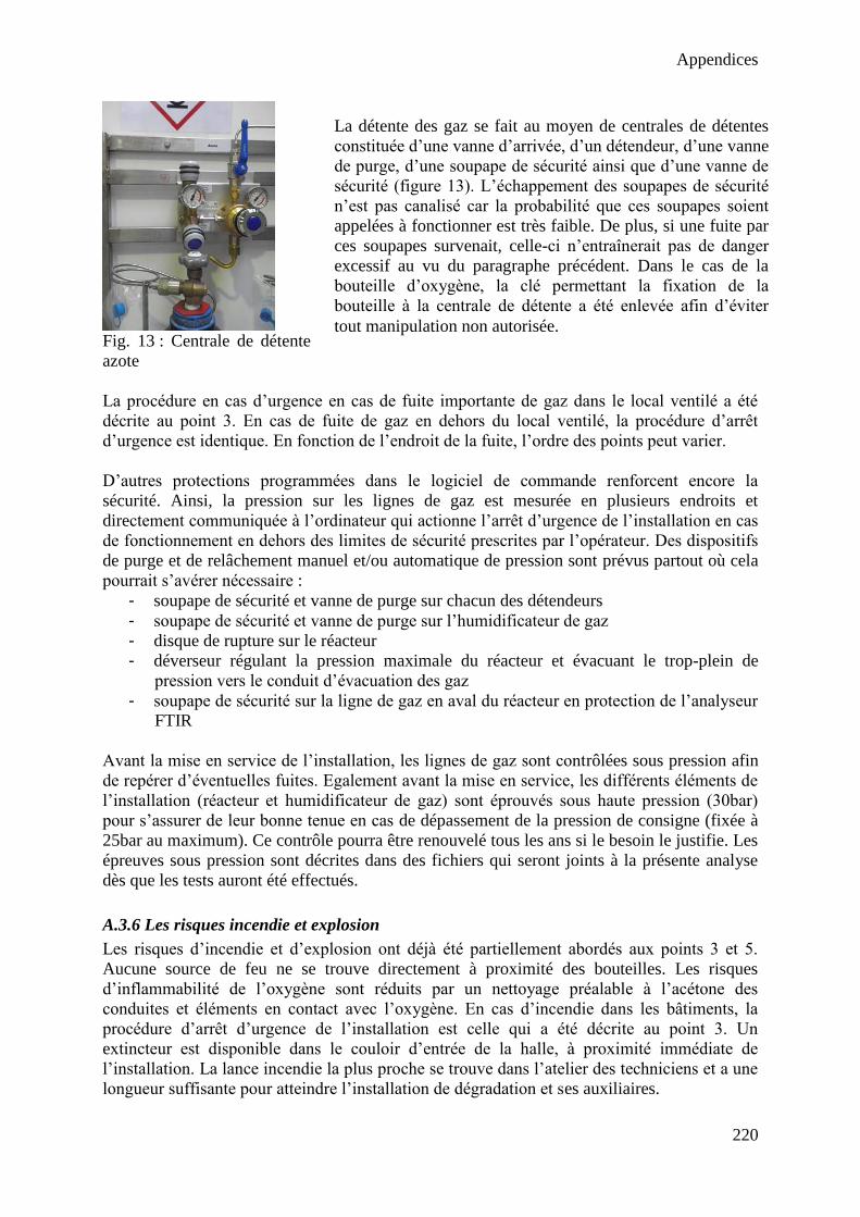
Appendices

220

Fig. 13 : Centrale de détente

azote

La procédure en cas d’urgence en cas de fuite importante de gaz dans le local ventilé a été

décrite au point 3. En cas de fuite de gaz en dehors du local ventilé, la procédure d’arrêt

d’urgence est identique. En fonction de l’endroit de la fuite, l’ordre des points peut varier.

D’autres protections programmées dans le logiciel de commande renforcent encore la

sécurité. Ainsi, la pression sur les lignes de gaz est mesurée en plusieurs endroits et

directement communiquée à l’ordinateur qui actionne l’arrêt d’urgence de l’installation en cas

de fonctionnement en dehors des limites de sécurité prescrites par l’opérateur. Des dispositifs

de purge et de relâchement manuel et/ou automatique de pression sont prévus partout où cela

pourrait s’avérer nécessaire :

- soupape de sécurité et vanne de purge sur chacun des détendeurs

- soupape de sécurité et vanne de purge sur l’humidificateur de gaz

- disque de rupture sur le réacteur

- déverseur régulant la pression maximale du réacteur et évacuant le trop-plein de

pression vers le conduit d’évacuation des gaz

- soupape de sécurité sur la ligne de gaz en aval du réacteur en protection de l’analyseur

FTIR

Avant la mise en service de l’installation, les lignes de gaz sont contrôlées sous pression afin

de repérer d’éventuelles fuites. Egalement avant la mise en service, les différents éléments de

l’installation (réacteur et humidificateur de gaz) sont éprouvés sous haute pression (30bar)

pour s’assurer de leur bonne tenue en cas de dépassement de la pression de consigne (fixée à

25bar au maximum). Ce contrôle pourra être renouvelé tous les ans si le besoin le justifie. Les

épreuves sous pression sont décrites dans des fichiers qui seront joints à la présente analyse

dès que les tests auront été effectués.

A.3.6 Les risques incendie et explosion

Les risques d’incendie et d’explosion ont déjà été partiellement abordés aux points 3 et 5.

Aucune source de feu ne se trouve directement à proximité des bouteilles. Les risques

d’inflammabilité de l’oxygène sont réduits par un nettoyage préalable à l’acétone des

conduites et éléments en contact avec l’oxygène. En cas d’incendie dans les bâtiments, la

procédure d’arrêt d’urgence de l’installation est celle qui a été décrite au point 3. Un

extincteur est disponible dans le couloir d’entrée de la halle, à proximité immédiate de

l’installation. La lance incendie la plus proche se trouve dans l’atelier des techniciens et a une

longueur suffisante pour atteindre l’installation de dégradation et ses auxiliaires.

La détente des gaz se fait au moyen de centrales de détentes

constituée d’une vanne d’arrivée, d’un détendeur, d’une vanne

de purge, d’une soupape de sécurité ainsi que d’une vanne de

sécurité (figure 13). L’échappement des soupapes de sécurité

n’est pas canalisé car la probabilité que ces soupapes soient

appelées à fonctionner est très faible. De plus, si une fuite par

ces soupapes survenait, celle-ci n’entraînerait pas de danger

excessif au vu du paragraphe précédent. Dans le cas de la

bouteille d’oxygène, la clé permettant la fixation de la

bouteille à la centrale de détente a été enlevée afin d’éviter

tout manipulation non autorisée.

Appendices

221

En cas de surpression dans le réacteur de dégradation ou sur les lignes de gaz périphériques au

réacteur, le risque d’explosion ne peut être négligé. En fonctionnement normal, la pression

maximale du réacteur est régulée par un déverseur qui évacue le trop-plein de pression vers le

conduit d’évacuation des gaz. Lors des expériences, la pression est mesurée en continu dans le

réacteur et à différents endroits des lignes de gaz. En cas de dépassement des valeurs limites

de sécurité prescrites par l’opérateur, le système informatique coupe automatiquement

l’arrivée de gaz au réacteur. Pour diminuer encore le risque lié à une défaillance informatique

ou mécanique, diverses précautions ont été prises :

- Manomètres placés sur le réacteur et sur le saturateur de gaz visibles à travers le

hublot depuis l’extérieur du local ventilé.

- Disque de rupture sur le réacteur calibré à 200 bars, dirigé vers le mur en cas de fuite

- Soupape de sécurité calibrée à 2.5 bars sur la ligne gaz en aval du réacteur pour

protéger l’analyseur FTIR. La sortie est redirigée vers un conduit d’aération en cas de

dépassement de la pression maximale admissible au FTIR.

- Soupape de sécurité calibrée à 40 bars sur le saturateur de gaz et dont la sortie est

dirigée vers le mur.

A.3.7 Le stockage des produits chimiques ou biologiques

La commande des produits chimiques se fait par l’intermédiaire du magasin de produits

chimiques de l’ULg. Les produits une fois arrivés sont stockés dans un endroit approprié pour

éviter toute dégradation de leur qualité. Le stockage et le transport des produits chimiques se

font en conservant l’emballage original de transport.

Selon les cas, le stockage se fait dans un frigo à proximité de l’installation ou dans une pièce

ventilée prévue à cet effet en dehors de la halle de chimie appliquée. La présence de produits

chimiques en dehors des lieux de stockage est limitée au strict nécessaire. La pièce ventilée

prévue pour le stockage des produits chimiques ne disposant pas d’un système d’aération

performant, il convient de patienter une à deux minutes entre l’ouverture de la porte de cette

pièce et l’entrée dans la pièce.

Les produits chimiques concernés ne présentent pas de risques particuliers lors de leur

stockage. Ils sont stockés par famille de risques. Leurs fiches de sécurité se trouvent dans la

farde de l’installation. Il n’y a pas manipulation de produits biologiques.

A.3.8 Le matériel de travail, les outils, les machines

Les surfaces de travail sont en bois traité de type « paillasse de laboratoire» et ne présentent

pas de risque de réaction avec les produits manipulés. Les outils de travail sont rangés dans

l’atelier des techniciens dans la halle de chimie appliquée. Leur état est régulièrement contrôlé

et les travailleurs sont suffisamment formés à leur utilisation.

A.3.9 Les commandes et signaux

Le panneau de contrôle de l’installation se situe juste à l’extérieur du local ventilé où se

trouve le réacteur de dégradation. L’ordinateur permet l’acquisition de données ainsi que le

contrôle des lignes de gaz. Un boitier de contrôle fourni avec le réacteur permet l’acquisition

de données ainsi que le contrôle du réacteur. Le panneau de contrôle peut être relié à internet

Appendices

222

de sorte que les données lues en direct puissent être consultables par un accès sécurisé depuis

n’importe quel ordinateur connecté à internet.

En cas de fonctionnement de l’installation en dehors des limites de sécurité prescrites par

l’opérateur, le système informatique coupe automatiquement l’alimentation en gaz du

réacteur. Le système de chauffe du réacteur est coupé automatiquement en cas de

dépassement des valeurs consignes de température et de pression au sein du réacteur.

A.3.10 Les positions de travail

L’installation étant prévue pour pouvoir fonctionner automatiquement, les principales

manipulations manuelles auront lieu entre les expériences. Lors du remplissage de

l’humidificateur de gaz au moyen d’eau distillée, il conviendra d’utiliser systématiquement un

entonnoir pour éviter de renverser de l’eau à proximité de l’installation et des fils électriques

environnants. Le réservoir de l’humidificateur sera toujours entièrement vidé avant

remplissage et le volume de remplissage sera toujours le même afin d’éviter tout débordement

d’eau. La fréquence de remplissage ne dépassera pas une fois tous les trois mois.

A.3.11 Les efforts et les manutentions

Pas d’effort ni de manutention spécifiques.

A.3.12 L’éclairage

L’éclairage du local ventilé se fait par lumière naturelle au travers d’une plaque de plastique

translucide au plafond du local. Un tube lumineux est également prévu, son interrupteur se

trouve en dehors du local ventilé, au-dessus de l’interrupteur pour l’aération. En dehors du

local ventilé, l’éclairage de la halle est suffisant pour le poste de contrôle.

En cas de coupure brusque de courant, un éclairage de secours situé à proximité de

l’installation prend le relais et éclaire le chemin vers la sortie. L’état de charge de cet

éclairage secondaire fonctionnant sur batterie est contrôlé régulièrement. De plus, une lampe

de poche se trouve dans l’atelier des techniciens dans un endroit facilement accessible dans le

noir.

A.3.13 Le bruit

Les principaux bruits sont ceux de la ventilation du local et de l’agitateur du réacteur. Ils sont

largement en-dessous des limites autorisées. En cas d’arrêt d’urgence de l’installation, les

vannes pneumatiques relâchent brusquement de l’air comprimé, laissant entendre un bruit

semblable à une détonation d’arme à feu. Afin d’éviter cela, des silencieux d’échappement ont

été rajoutés.

A.3.14 Les ambiances thermiques

La température est celle de la Halle de Chimie Appliquée. Un système de chauffage est prévu

pour l’hiver mais ne fonctionne qu’en mode anti-gel en dehors des heures d’ouverture de la

Halle. Il n’y a pas de climatisation en été, mais si nécessaire, les portes de la halle sont

maintenues ouvertes pour permettre une circulation supplémentaire d’air. Aucun problème lié

à l’humidité n’a été constaté.

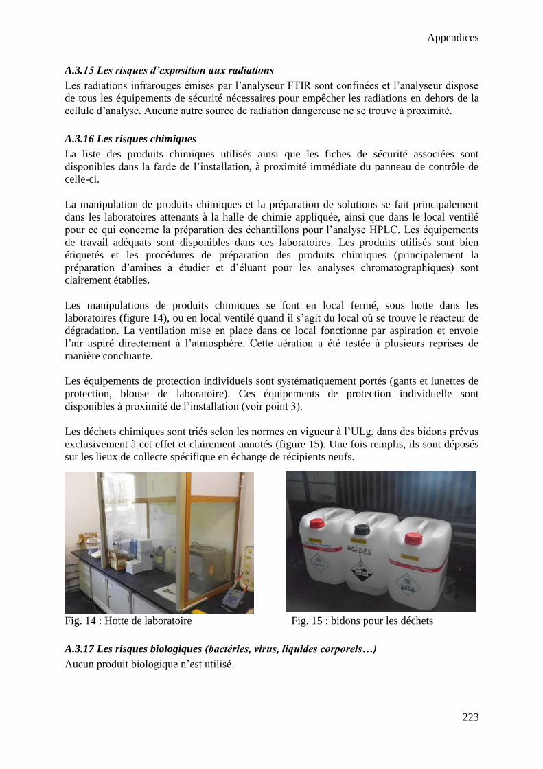
Appendices

223

A.3.15 Les risques d’exposition aux radiations

Les radiations infrarouges émises par l’analyseur FTIR sont confinées et l’analyseur dispose

de tous les équipements de sécurité nécessaires pour empêcher les radiations en dehors de la

cellule d’analyse. Aucune autre source de radiation dangereuse ne se trouve à proximité.

A.3.16 Les risques chimiques

La liste des produits chimiques utilisés ainsi que les fiches de sécurité associées sont

disponibles dans la farde de l’installation, à proximité immédiate du panneau de contrôle de

celle-ci.

La manipulation de produits chimiques et la préparation de solutions se fait principalement

dans les laboratoires attenants à la halle de chimie appliquée, ainsi que dans le local ventilé

pour ce qui concerne la préparation des échantillons pour l’analyse HPLC. Les équipements

de travail adéquats sont disponibles dans ces laboratoires. Les produits utilisés sont bien

étiquetés et les procédures de préparation des produits chimiques (principalement la

préparation d’amines à étudier et d’éluant pour les analyses chromatographiques) sont

clairement établies.

Les manipulations de produits chimiques se font en local fermé, sous hotte dans les

laboratoires (figure 14), ou en local ventilé quand il s’agit du local où se trouve le réacteur de

dégradation. La ventilation mise en place dans ce local fonctionne par aspiration et envoie

l’air aspiré directement à l’atmosphère. Cette aération a été testée à plusieurs reprises de

manière concluante.

Les équipements de protection individuels sont systématiquement portés (gants et lunettes de

protection, blouse de laboratoire). Ces équipements de protection individuelle sont

disponibles à proximité de l’installation (voir point 3).

Les déchets chimiques sont triés selon les normes en vigueur à l’ULg, dans des bidons prévus

exclusivement à cet effet et clairement annotés (figure 15). Une fois remplis, ils sont déposés

sur les lieux de collecte spécifique en échange de récipients neufs.

Fig. 14 : Hotte de laboratoire Fig. 15 : bidons pour les déchets

A.3.17 Les risques biologiques (bactéries, virus, liquides corporels…)

Aucun produit biologique n’est utilisé.

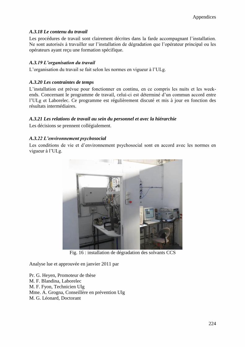
Appendices

224

A.3.18 Le contenu du travail

Les procédures de travail sont clairement décrites dans la farde accompagnant l’installation.

Ne sont autorisés à travailler sur l’installation de dégradation que l’opérateur principal ou les

opérateurs ayant reçu une formation spécifique.

A.3.19 L’organisation du travail

L’organisation du travail se fait selon les normes en vigueur à l’ULg.

A.3.20 Les contraintes de temps

L’installation est prévue pour fonctionner en continu, en ce compris les nuits et les week-

ends. Concernant le programme de travail, celui-ci est déterminé d’un commun accord entre

l’ULg et Laborelec. Ce programme est régulièrement discuté et mis à jour en fonction des

résultats intermédiaires.

A.3.21 Les relations de travail au sein du personnel et avec la hiérarchie

Les décisions se prennent collégialement.

A.3.22 L’environnement psychosocial

Les conditions de vie et d’environnement psychosocial sont en accord avec les normes en

vigueur à l’ULg.

Fig. 16 : installation de dégradation des solvants CCS

Analyse lue et approuvée en janvier 2011 par

Pr. G. Heyen, Promoteur de thèse

M. F. Blandina, Laborelec

M. F. Fyon, Technicien Ulg

Mme. A. Grogna, Conseillère en prévention Ulg

M. G. Léonard, Doctorant

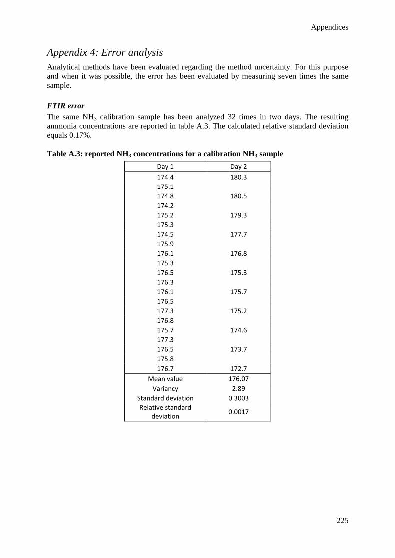
Appendices

225

Appendix 4: Error analysis

Analytical methods have been evaluated regarding the method uncertainty. For this purpose

and when it was possible, the error has been evaluated by measuring seven times the same

sample.

FTIR error

The same NH3 calibration sample has been analyzed 32 times in two days. The resulting

ammonia concentrations are reported in table A.3. The calculated relative standard deviation

equals 0.17%.

Table A.3: reported NH3 concentrations for a calibration NH3 sample

Day 1 Day 2

174.4 180.3

175.1

174.8 180.5

174.2

175.2 179.3

175.3

174.5 177.7

175.9

176.1 176.8

175.3

176.5 175.3

176.3

176.1 175.7

176.5

177.3 175.2

176.8

175.7 174.6

177.3

176.5 173.7

175.8

176.7 172.7

Mean value 176.07

Variancy 2.89

Standard deviation 0.3003

Relative standard deviation

0.0017

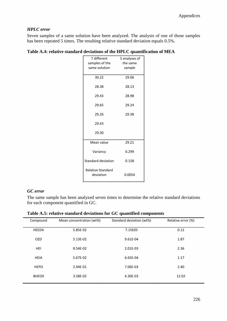
Appendices

226

HPLC error

Seven samples of a same solution have been analyzed. The analysis of one of those samples

has been repeated 5 times. The resulting relative standard deviation equals 0.5%.

Table A.4: relative standard deviations of the HPLC quantification of MEA

7 different samples of the same solution

5 analyses of the same sample

30.22 29.06

28.38 28.13

29.43 28.98

29.65 29.24

29.26 29.38

29.43

29.30

Mean value 29.21

Variancy 0.299

Standard deviation 0.158

Relative Standard deviation 0.0054

GC error

The same sample has been analyzed seven times to determine the relative standard deviations

for each component quantified in GC.

Table A.5: relative standard deviations for GC quantified components

Compound Mean concentration (wt%) Standard deviation (wt%) Relative error (%)

HEEDA 5.85E-02 7.15E05 0.12

OZD 5.13E-02 9.61E-04 1.87

HEI 8.54E-02 2.01E-03 2.36

HEIA 5.67E-02 6.65E-04 1.17

HEPO 2.94E-01 7.06E-03 2.40

BHEOX 3.58E-02 4.30E-03 12.02

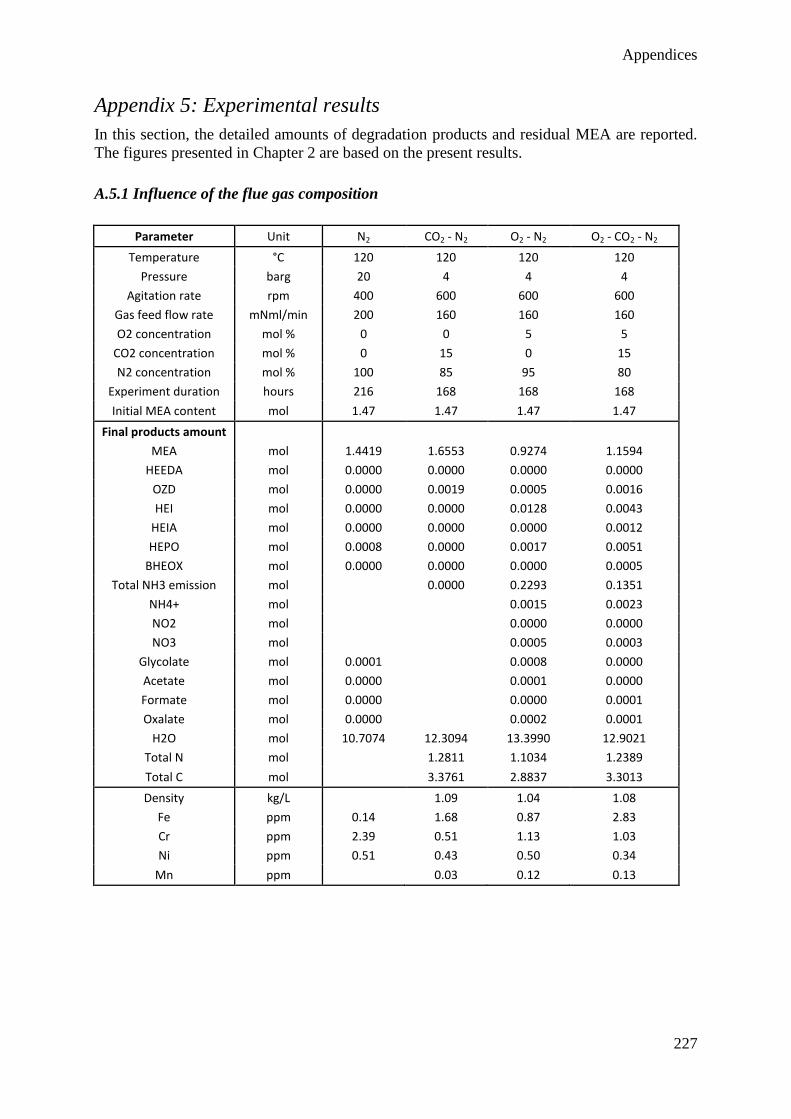
Appendices

227

Appendix 5: Experimental results

In this section, the detailed amounts of degradation products and residual MEA are reported.

The figures presented in Chapter 2 are based on the present results.

A.5.1 Influence of the flue gas composition

Parameter Unit N2 CO2 - N2 O2 - N2 O2 - CO2 - N2

Temperature °C 120 120 120 120

Pressure barg 20 4 4 4

Agitation rate rpm 400 600 600 600

Gas feed flow rate mNml/min 200 160 160 160

O2 concentration mol % 0 0 5 5

CO2 concentration mol % 0 15 0 15

N2 concentration mol % 100 85 95 80

Experiment duration hours 216 168 168 168

Initial MEA content mol 1.47 1.47 1.47 1.47

Final products amount

MEA mol 1.4419 1.6553 0.9274 1.1594

HEEDA mol 0.0000 0.0000 0.0000 0.0000

OZD mol 0.0000 0.0019 0.0005 0.0016

HEI mol 0.0000 0.0000 0.0128 0.0043

HEIA mol 0.0000 0.0000 0.0000 0.0012

HEPO mol 0.0008 0.0000 0.0017 0.0051

BHEOX mol 0.0000 0.0000 0.0000 0.0005

Total NH3 emission mol 0.0000 0.2293 0.1351

NH4+ mol

0.0015 0.0023

NO2 mol

0.0000 0.0000

NO3 mol

0.0005 0.0003

Glycolate mol 0.0001

0.0008 0.0000

Acetate mol 0.0000

0.0001 0.0000

Formate mol 0.0000

0.0000 0.0001

Oxalate mol 0.0000

0.0002 0.0001

H2O mol 10.7074 12.3094 13.3990 12.9021

Total N mol 1.2811 1.1034 1.2389

Total C mol 3.3761 2.8837 3.3013

Density kg/L 1.09 1.04 1.08

Fe ppm 0.14 1.68 0.87 2.83

Cr ppm 2.39 0.51 1.13 1.03

Ni ppm 0.51 0.43 0.50 0.34

Mn ppm 0.03 0.12 0.13

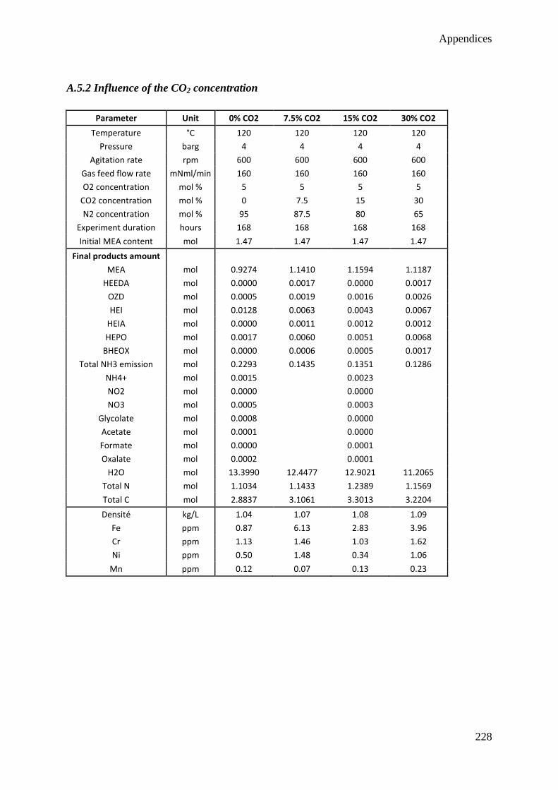
Appendices

228

A.5.2 Influence of the CO2 concentration

Parameter Unit 0% CO2 7.5% CO2 15% CO2 30% CO2

Temperature °C 120 120 120 120

Pressure barg 4 4 4 4

Agitation rate rpm 600 600 600 600

Gas feed flow rate mNml/min 160 160 160 160

O2 concentration mol % 5 5 5 5

CO2 concentration mol % 0 7.5 15 30

N2 concentration mol % 95 87.5 80 65

Experiment duration hours 168 168 168 168

Initial MEA content mol 1.47 1.47 1.47 1.47

Final products amount

MEA mol 0.9274 1.1410 1.1594 1.1187

HEEDA mol 0.0000 0.0017 0.0000 0.0017

OZD mol 0.0005 0.0019 0.0016 0.0026

HEI mol 0.0128 0.0063 0.0043 0.0067

HEIA mol 0.0000 0.0011 0.0012 0.0012

HEPO mol 0.0017 0.0060 0.0051 0.0068

BHEOX mol 0.0000 0.0006 0.0005 0.0017

Total NH3 emission mol 0.2293 0.1435 0.1351 0.1286

NH4+ mol 0.0015

0.0023

NO2 mol 0.0000

0.0000

NO3 mol 0.0005

0.0003

Glycolate mol 0.0008

0.0000

Acetate mol 0.0001

0.0000

Formate mol 0.0000

0.0001

Oxalate mol 0.0002

0.0001

H2O mol 13.3990 12.4477 12.9021 11.2065

Total N mol 1.1034 1.1433 1.2389 1.1569

Total C mol 2.8837 3.1061 3.3013 3.2204

Densité kg/L 1.04 1.07 1.08 1.09

Fe ppm 0.87 6.13 2.83 3.96

Cr ppm 1.13 1.46 1.03 1.62

Ni ppm 0.50 1.48 0.34 1.06

Mn ppm 0.12 0.07 0.13 0.23

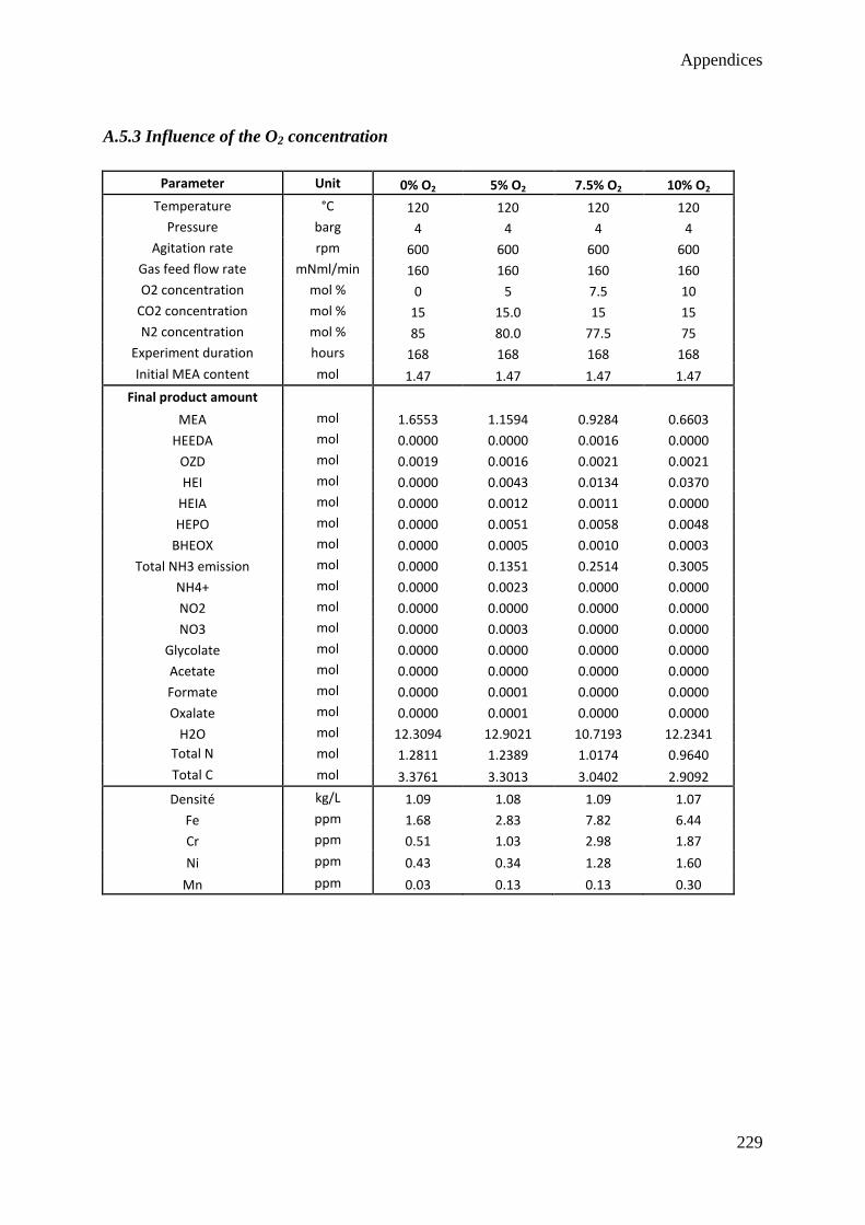
Appendices

229

A.5.3 Influence of the O2 concentration

Parameter Unit 0% O2 5% O2 7.5% O2 10% O2

Temperature °C 120 120 120 120

Pressure barg 4 4 4 4

Agitation rate rpm 600 600 600 600

Gas feed flow rate mNml/min 160 160 160 160

O2 concentration mol % 0 5 7.5 10

CO2 concentration mol % 15 15.0 15 15

N2 concentration mol % 85 80.0 77.5 75

Experiment duration hours 168 168 168 168

Initial MEA content mol 1.47 1.47 1.47 1.47

Final product amount

MEA mol 1.6553 1.1594 0.9284 0.6603

HEEDA mol 0.0000 0.0000 0.0016 0.0000

OZD mol 0.0019 0.0016 0.0021 0.0021

HEI mol 0.0000 0.0043 0.0134 0.0370

HEIA mol 0.0000 0.0012 0.0011 0.0000

HEPO mol 0.0000 0.0051 0.0058 0.0048

BHEOX mol 0.0000 0.0005 0.0010 0.0003

Total NH3 emission mol 0.0000 0.1351 0.2514 0.3005

NH4+ mol 0.0000 0.0023 0.0000 0.0000

NO2 mol 0.0000 0.0000 0.0000 0.0000

NO3 mol 0.0000 0.0003 0.0000 0.0000

Glycolate mol 0.0000 0.0000 0.0000 0.0000

Acetate mol 0.0000 0.0000 0.0000 0.0000

Formate mol 0.0000 0.0001 0.0000 0.0000

Oxalate mol 0.0000 0.0001 0.0000 0.0000

H2O mol 12.3094 12.9021 10.7193 12.2341

Total N mol 1.2811 1.2389 1.0174 0.9640

Total C mol 3.3761 3.3013 3.0402 2.9092

Densité kg/L 1.09 1.08 1.09 1.07

Fe ppm 1.68 2.83 7.82 6.44

Cr ppm 0.51 1.03 2.98 1.87

Ni ppm 0.43 0.34 1.28 1.60

Mn ppm 0.03 0.13 0.13 0.30

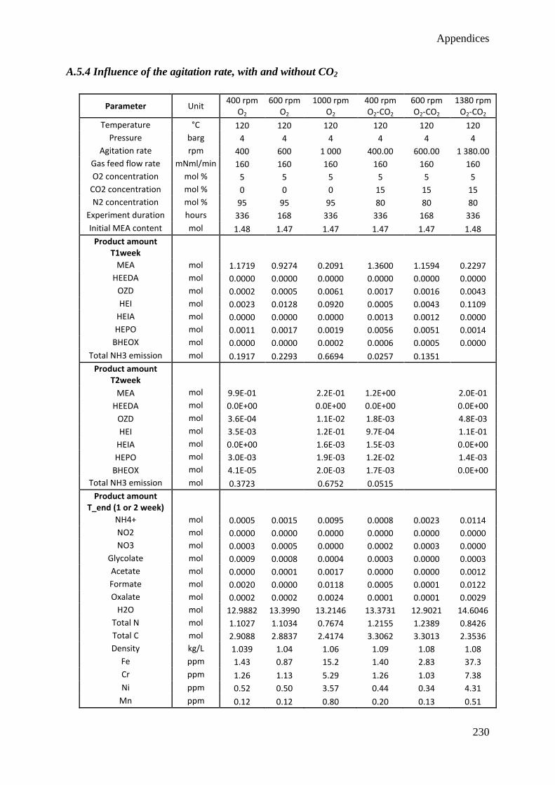
Appendices

230

A.5.4 Influence of the agitation rate, with and without CO2

Parameter Unit 400 rpm

O2 600 rpm

O2 1000 rpm

O2 400 rpm O2-CO2

600 rpm O2-CO2

1380 rpm O2-CO2

Temperature °C 120 120 120 120 120 120

Pressure barg 4 4 4 4 4 4

Agitation rate rpm 400 600 1 000 400.00 600.00 1 380.00

Gas feed flow rate mNml/min 160 160 160 160 160 160

O2 concentration mol % 5 5 5 5 5 5

CO2 concentration mol % 0 0 0 15 15 15

N2 concentration mol % 95 95 95 80 80 80

Experiment duration hours 336 168 336 336 168 336

Initial MEA content mol 1.48 1.47 1.47 1.47 1.47 1.48

Product amount T1week

MEA mol 1.1719 0.9274 0.2091 1.3600 1.1594 0.2297

HEEDA mol 0.0000 0.0000 0.0000 0.0000 0.0000 0.0000

OZD mol 0.0002 0.0005 0.0061 0.0017 0.0016 0.0043

HEI mol 0.0023 0.0128 0.0920 0.0005 0.0043 0.1109

HEIA mol 0.0000 0.0000 0.0000 0.0013 0.0012 0.0000

HEPO mol 0.0011 0.0017 0.0019 0.0056 0.0051 0.0014

BHEOX mol 0.0000 0.0000 0.0002 0.0006 0.0005 0.0000

Total NH3 emission mol 0.1917 0.2293 0.6694 0.0257 0.1351

Product amount T2week

MEA mol 9.9E-01

2.2E-01 1.2E+00

2.0E-01

HEEDA mol 0.0E+00

0.0E+00 0.0E+00

0.0E+00

OZD mol 3.6E-04

1.1E-02 1.8E-03

4.8E-03

HEI mol 3.5E-03

1.2E-01 9.7E-04

1.1E-01

HEIA mol 0.0E+00

1.6E-03 1.5E-03

0.0E+00

HEPO mol 3.0E-03

1.9E-03 1.2E-02

1.4E-03

BHEOX mol 4.1E-05

2.0E-03 1.7E-03

0.0E+00

Total NH3 emission mol 0.3723 0.6752 0.0515

Product amount T_end (1 or 2 week)

NH4+ mol 0.0005 0.0015 0.0095 0.0008 0.0023 0.0114

NO2 mol 0.0000 0.0000 0.0000 0.0000 0.0000 0.0000

NO3 mol 0.0003 0.0005 0.0000 0.0002 0.0003 0.0000

Glycolate mol 0.0009 0.0008 0.0004 0.0003 0.0000 0.0003

Acetate mol 0.0000 0.0001 0.0017 0.0000 0.0000 0.0012

Formate mol 0.0020 0.0000 0.0118 0.0005 0.0001 0.0122

Oxalate mol 0.0002 0.0002 0.0024 0.0001 0.0001 0.0029

H2O mol 12.9882 13.3990 13.2146 13.3731 12.9021 14.6046

Total N mol 1.1027 1.1034 0.7674 1.2155 1.2389 0.8426

Total C mol 2.9088 2.8837 2.4174 3.3062 3.3013 2.3536

Density kg/L 1.039 1.04 1.06 1.09 1.08 1.08

Fe ppm 1.43 0.87 15.2 1.40 2.83 37.3

Cr ppm 1.26 1.13 5.29 1.26 1.03 7.38

Ni ppm 0.52 0.50 3.57 0.44 0.34 4.31

Mn ppm 0.12 0.12 0.80 0.20 0.13 0.51

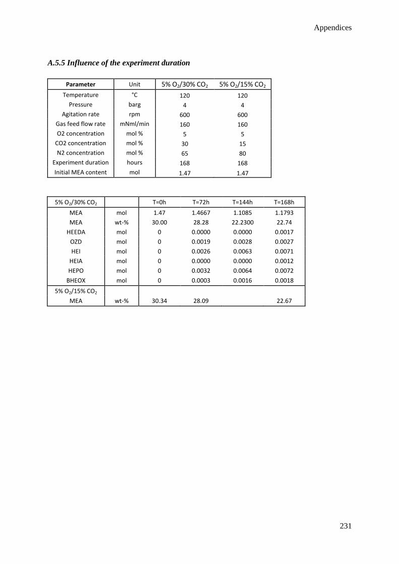
Appendices

231

A.5.5 Influence of the experiment duration

Parameter Unit 5% O2/30% CO2 5% O2/15% CO2

Temperature °C 120 120

Pressure barg 4 4

Agitation rate rpm 600 600

Gas feed flow rate mNml/min 160 160

O2 concentration mol % 5 5

CO2 concentration mol % 30 15

N2 concentration mol % 65 80

Experiment duration hours 168 168

Initial MEA content mol 1.47 1.47

5% O2/30% CO2 T=0h T=72h T=144h T=168h

MEA mol 1.47 1.4667 1.1085 1.1793

MEA wt-% 30.00 28.28 22.2300 22.74

HEEDA mol 0 0.0000 0.0000 0.0017

OZD mol 0 0.0019 0.0028 0.0027

HEI mol 0 0.0026 0.0063 0.0071

HEIA mol 0 0.0000 0.0000 0.0012

HEPO mol 0 0.0032 0.0064 0.0072

BHEOX mol 0 0.0003 0.0016 0.0018

5% O2/15% CO2

MEA wt-% 30.34 28.09 22.67

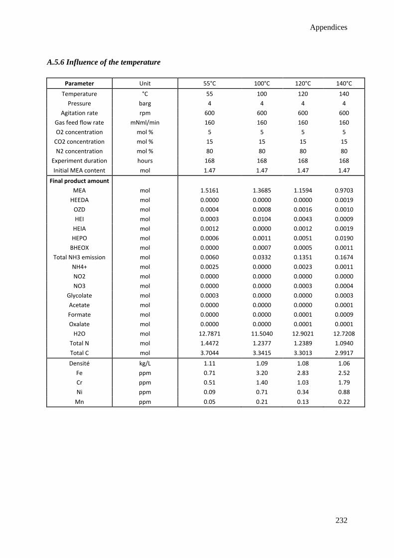
Appendices

232

A.5.6 Influence of the temperature

Parameter Unit 55°C 100°C 120°C 140°C

Temperature °C 55 100 120 140

Pressure barg 4 4 4 4

Agitation rate rpm 600 600 600 600

Gas feed flow rate mNml/min 160 160 160 160

O2 concentration mol % 5 5 5 5

CO2 concentration mol % 15 15 15 15

N2 concentration mol % 80 80 80 80

Experiment duration hours 168 168 168 168

Initial MEA content mol 1.47 1.47 1.47 1.47

Final product amount

MEA mol 1.5161 1.3685 1.1594 0.9703

HEEDA mol 0.0000 0.0000 0.0000 0.0019

OZD mol 0.0004 0.0008 0.0016 0.0010

HEI mol 0.0003 0.0104 0.0043 0.0009

HEIA mol 0.0012 0.0000 0.0012 0.0019

HEPO mol 0.0006 0.0011 0.0051 0.0190

BHEOX mol 0.0000 0.0007 0.0005 0.0011

Total NH3 emission mol 0.0060 0.0332 0.1351 0.1674

NH4+ mol 0.0025 0.0000 0.0023 0.0011

NO2 mol 0.0000 0.0000 0.0000 0.0000

NO3 mol 0.0000 0.0000 0.0003 0.0004

Glycolate mol 0.0003 0.0000 0.0000 0.0003

Acetate mol 0.0000 0.0000 0.0000 0.0001

Formate mol 0.0000 0.0000 0.0001 0.0009

Oxalate mol 0.0000 0.0000 0.0001 0.0001

H2O mol 12.7871 11.5040 12.9021 12.7208

Total N mol 1.4472 1.2377 1.2389 1.0940

Total C mol 3.7044 3.3415 3.3013 2.9917

Densité kg/L 1.11 1.09 1.08 1.06

Fe ppm 0.71 3.20 2.83 2.52

Cr ppm 0.51 1.40 1.03 1.79

Ni ppm 0.09 0.71 0.34 0.88

Mn ppm 0.05 0.21 0.13 0.22

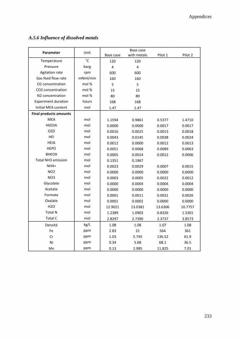
Appendices

233

A.5.6 Influence of dissolved metals

Parameter Unit Base case

Base case with metals Pilot 1 Pilot 2

Temperature °C 120 120

Pressure barg 4 4

Agitation rate rpm 600 600

Gas feed flow rate mNml/min 160 160

O2 concentration mol % 5 5

CO2 concentration mol % 15 15

N2 concentration mol % 80 80

Experiment duration hours 168 168

Initial MEA content mol 1.47 1.47

Final products amounts

MEA mol 1.1594 0.9861 0.5377 1.4710

HEEDA mol 0.0000 0.0000 0.0017 0.0017

OZD mol 0.0016 0.0025 0.0013 0.0018

HEI mol 0.0043 0.0145 0.0038 0.0024

HEIA mol 0.0012 0.0000 0.0012 0.0013

HEPO mol 0.0051 0.0068 0.0089 0.0063

BHEOX mol 0.0005 0.0014 0.0012 0.0006

Total NH3 emission mol 0.1351 0.1967

NH4+ mol 0.0023 0.0029 0.0007 0.0015

NO2 mol 0.0000 0.0000 0.0000 0.0000

NO3 mol 0.0003 0.0005 0.0022 0.0012

Glycolate mol 0.0000 0.0004 0.0004 0.0004

Acetate mol 0.0000 0.0000 0.0000 0.0000

Formate mol 0.0001 0.0011 0.0031 0.0026

Oxalate mol 0.0001 0.0002 0.0000 0.0000

H2O mol 12.9021 13.0381 13.6306 10.7757

Total N mol 1.2389 1.0903 0.8326 1.5301

Total C mol 2.8297 2.7390 2.3737 3.8573

Densité kg/L 1.08 1.08 1.07 1.08

Fe ppm 2.83 21 564 361

Cr ppm 1.03 5.745 136.52 61.9

Ni ppm 0.34 5.68 68.1 36.5

Mn ppm 0.13 2.985 11.825 7.01

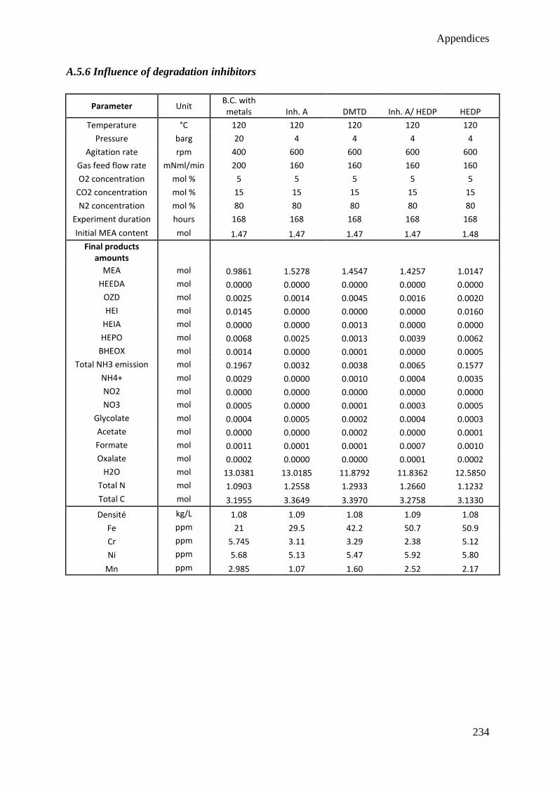
Appendices

234

A.5.6 Influence of degradation inhibitors

Parameter Unit B.C. with metals Inh. A DMTD Inh. A/ HEDP HEDP

Temperature °C 120 120 120 120 120

Pressure barg 20 4 4 4 4

Agitation rate rpm 400 600 600 600 600

Gas feed flow rate mNml/min 200 160 160 160 160

O2 concentration mol % 5 5 5 5 5

CO2 concentration mol % 15 15 15 15 15

N2 concentration mol % 80 80 80 80 80

Experiment duration hours 168 168 168 168 168

Initial MEA content mol 1.47 1.47 1.47 1.47 1.48

Final products amounts

MEA mol 0.9861 1.5278 1.4547 1.4257 1.0147

HEEDA mol 0.0000 0.0000 0.0000 0.0000 0.0000

OZD mol 0.0025 0.0014 0.0045 0.0016 0.0020

HEI mol 0.0145 0.0000 0.0000 0.0000 0.0160

HEIA mol 0.0000 0.0000 0.0013 0.0000 0.0000

HEPO mol 0.0068 0.0025 0.0013 0.0039 0.0062

BHEOX mol 0.0014 0.0000 0.0001 0.0000 0.0005

Total NH3 emission mol 0.1967 0.0032 0.0038 0.0065 0.1577

NH4+ mol 0.0029 0.0000 0.0010 0.0004 0.0035

NO2 mol 0.0000 0.0000 0.0000 0.0000 0.0000

NO3 mol 0.0005 0.0000 0.0001 0.0003 0.0005

Glycolate mol 0.0004 0.0005 0.0002 0.0004 0.0003

Acetate mol 0.0000 0.0000 0.0002 0.0000 0.0001

Formate mol 0.0011 0.0001 0.0001 0.0007 0.0010

Oxalate mol 0.0002 0.0000 0.0000 0.0001 0.0002

H2O mol 13.0381 13.0185 11.8792 11.8362 12.5850

Total N mol 1.0903 1.2558 1.2933 1.2660 1.1232

Total C mol 3.1955 3.3649 3.3970 3.2758 3.1330

Densité kg/L 1.08 1.09 1.08 1.09 1.08

Fe ppm 21 29.5 42.2 50.7 50.9

Cr ppm 5.745 3.11 3.29 2.38 5.12

Ni ppm 5.68 5.13 5.47 5.92 5.80

Mn ppm 2.985 1.07 1.60 2.52 2.17

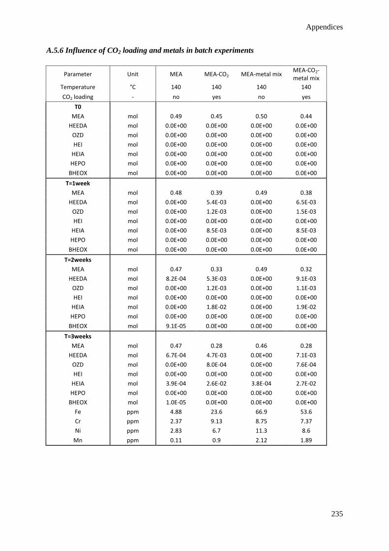
Appendices

235

A.5.6 Influence of CO2 loading and metals in batch experiments

Parameter Unit MEA MEA-CO2 MEA-metal mix MEA-CO2-metal mix

Temperature °C 140 140 140 140

CO2 loading - no yes no yes

T0

MEA mol 0.49 0.45 0.50 0.44

HEEDA mol 0.0E+00 0.0E+00 0.0E+00 0.0E+00

OZD mol 0.0E+00 0.0E+00 0.0E+00 0.0E+00

HEI mol 0.0E+00 0.0E+00 0.0E+00 0.0E+00

HEIA mol 0.0E+00 0.0E+00 0.0E+00 0.0E+00

HEPO mol 0.0E+00 0.0E+00 0.0E+00 0.0E+00

BHEOX mol 0.0E+00 0.0E+00 0.0E+00 0.0E+00

T=1week

MEA mol 0.48 0.39 0.49 0.38

HEEDA mol 0.0E+00 5.4E-03 0.0E+00 6.5E-03

OZD mol 0.0E+00 1.2E-03 0.0E+00 1.5E-03

HEI mol 0.0E+00 0.0E+00 0.0E+00 0.0E+00

HEIA mol 0.0E+00 8.5E-03 0.0E+00 8.5E-03

HEPO mol 0.0E+00 0.0E+00 0.0E+00 0.0E+00

BHEOX mol 0.0E+00 0.0E+00 0.0E+00 0.0E+00

T=2weeks

MEA mol 0.47 0.33 0.49 0.32

HEEDA mol 8.2E-04 5.3E-03 0.0E+00 9.1E-03

OZD mol 0.0E+00 1.2E-03 0.0E+00 1.1E-03

HEI mol 0.0E+00 0.0E+00 0.0E+00 0.0E+00

HEIA mol 0.0E+00 1.8E-02 0.0E+00 1.9E-02

HEPO mol 0.0E+00 0.0E+00 0.0E+00 0.0E+00

BHEOX mol 9.1E-05 0.0E+00 0.0E+00 0.0E+00

T=3weeks

MEA mol 0.47 0.28 0.46 0.28

HEEDA mol 6.7E-04 4.7E-03 0.0E+00 7.1E-03

OZD mol 0.0E+00 8.0E-04 0.0E+00 7.6E-04

HEI mol 0.0E+00 0.0E+00 0.0E+00 0.0E+00

HEIA mol 3.9E-04 2.6E-02 3.8E-04 2.7E-02

HEPO mol 0.0E+00 0.0E+00 0.0E+00 0.0E+00

BHEOX mol 1.0E-05 0.0E+00 0.0E+00 0.0E+00

Fe ppm 4.88 23.6 66.9 53.6

Cr ppm 2.37 9.13 8.75 7.37

Ni ppm 2.83 6.7 11.3 8.6

Mn ppm 0.11 0.9 2.12 1.89

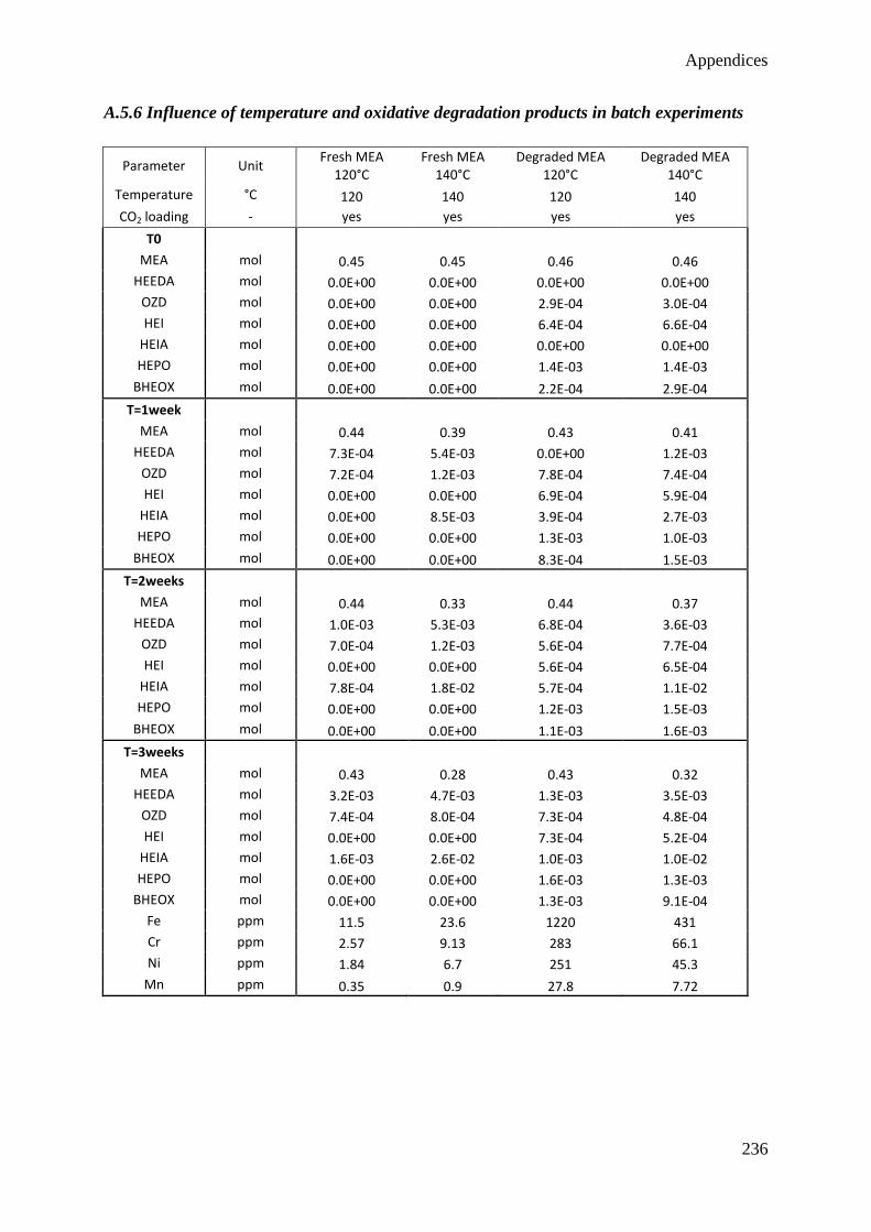
Appendices

236

A.5.6 Influence of temperature and oxidative degradation products in batch experiments

Parameter Unit Fresh MEA

120°C Fresh MEA

140°C Degraded MEA

120°C Degraded MEA

140°C

Temperature °C 120 140 120 140

CO2 loading - yes yes yes yes

T0

MEA mol 0.45 0.45 0.46 0.46

HEEDA mol 0.0E+00 0.0E+00 0.0E+00 0.0E+00

OZD mol 0.0E+00 0.0E+00 2.9E-04 3.0E-04

HEI mol 0.0E+00 0.0E+00 6.4E-04 6.6E-04

HEIA mol 0.0E+00 0.0E+00 0.0E+00 0.0E+00

HEPO mol 0.0E+00 0.0E+00 1.4E-03 1.4E-03

BHEOX mol 0.0E+00 0.0E+00 2.2E-04 2.9E-04

T=1week

MEA mol 0.44 0.39 0.43 0.41

HEEDA mol 7.3E-04 5.4E-03 0.0E+00 1.2E-03

OZD mol 7.2E-04 1.2E-03 7.8E-04 7.4E-04

HEI mol 0.0E+00 0.0E+00 6.9E-04 5.9E-04

HEIA mol 0.0E+00 8.5E-03 3.9E-04 2.7E-03

HEPO mol 0.0E+00 0.0E+00 1.3E-03 1.0E-03

BHEOX mol 0.0E+00 0.0E+00 8.3E-04 1.5E-03

T=2weeks

MEA mol 0.44 0.33 0.44 0.37

HEEDA mol 1.0E-03 5.3E-03 6.8E-04 3.6E-03

OZD mol 7.0E-04 1.2E-03 5.6E-04 7.7E-04

HEI mol 0.0E+00 0.0E+00 5.6E-04 6.5E-04

HEIA mol 7.8E-04 1.8E-02 5.7E-04 1.1E-02

HEPO mol 0.0E+00 0.0E+00 1.2E-03 1.5E-03

BHEOX mol 0.0E+00 0.0E+00 1.1E-03 1.6E-03

T=3weeks

MEA mol 0.43 0.28 0.43 0.32

HEEDA mol 3.2E-03 4.7E-03 1.3E-03 3.5E-03

OZD mol 7.4E-04 8.0E-04 7.3E-04 4.8E-04

HEI mol 0.0E+00 0.0E+00 7.3E-04 5.2E-04

HEIA mol 1.6E-03 2.6E-02 1.0E-03 1.0E-02

HEPO mol 0.0E+00 0.0E+00 1.6E-03 1.3E-03

BHEOX mol 0.0E+00 0.0E+00 1.3E-03 9.1E-04

Fe ppm 11.5 23.6 1220 431

Cr ppm 2.57 9.13 283 66.1

Ni ppm 1.84 6.7 251 45.3

Mn ppm 0.35 0.9 27.8 7.72

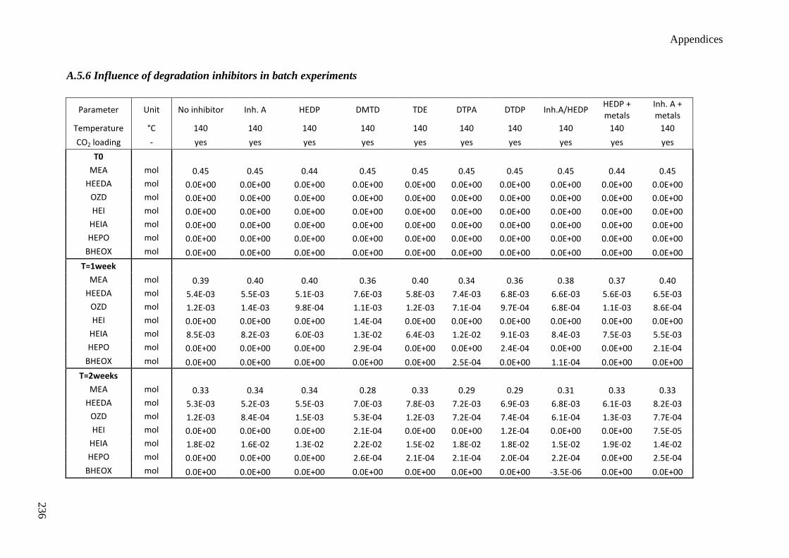
Appendices

236

A.5.6 Influence of degradation inhibitors in batch experiments

Parameter Unit No inhibitor Inh. A HEDP DMTD TDE DTPA DTDP Inh.A/HEDP HEDP + metals

Inh. A + metals

Temperature °C 140 140 140 140 140 140 140 140 140 140

CO2 loading - yes yes yes yes yes yes yes yes yes yes

T0

MEA mol 0.45 0.45 0.44 0.45 0.45 0.45 0.45 0.45 0.44 0.45

HEEDA mol 0.0E+00 0.0E+00 0.0E+00 0.0E+00 0.0E+00 0.0E+00 0.0E+00 0.0E+00 0.0E+00 0.0E+00

OZD mol 0.0E+00 0.0E+00 0.0E+00 0.0E+00 0.0E+00 0.0E+00 0.0E+00 0.0E+00 0.0E+00 0.0E+00

HEI mol 0.0E+00 0.0E+00 0.0E+00 0.0E+00 0.0E+00 0.0E+00 0.0E+00 0.0E+00 0.0E+00 0.0E+00

HEIA mol 0.0E+00 0.0E+00 0.0E+00 0.0E+00 0.0E+00 0.0E+00 0.0E+00 0.0E+00 0.0E+00 0.0E+00

HEPO mol 0.0E+00 0.0E+00 0.0E+00 0.0E+00 0.0E+00 0.0E+00 0.0E+00 0.0E+00 0.0E+00 0.0E+00

BHEOX mol 0.0E+00 0.0E+00 0.0E+00 0.0E+00 0.0E+00 0.0E+00 0.0E+00 0.0E+00 0.0E+00 0.0E+00

T=1week

MEA mol 0.39 0.40 0.40 0.36 0.40 0.34 0.36 0.38 0.37 0.40

HEEDA mol 5.4E-03 5.5E-03 5.1E-03 7.6E-03 5.8E-03 7.4E-03 6.8E-03 6.6E-03 5.6E-03 6.5E-03

OZD mol 1.2E-03 1.4E-03 9.8E-04 1.1E-03 1.2E-03 7.1E-04 9.7E-04 6.8E-04 1.1E-03 8.6E-04

HEI mol 0.0E+00 0.0E+00 0.0E+00 1.4E-04 0.0E+00 0.0E+00 0.0E+00 0.0E+00 0.0E+00 0.0E+00

HEIA mol 8.5E-03 8.2E-03 6.0E-03 1.3E-02 6.4E-03 1.2E-02 9.1E-03 8.4E-03 7.5E-03 5.5E-03

HEPO mol 0.0E+00 0.0E+00 0.0E+00 2.9E-04 0.0E+00 0.0E+00 2.4E-04 0.0E+00 0.0E+00 2.1E-04

BHEOX mol 0.0E+00 0.0E+00 0.0E+00 0.0E+00 0.0E+00 2.5E-04 0.0E+00 1.1E-04 0.0E+00 0.0E+00

T=2weeks

MEA mol 0.33 0.34 0.34 0.28 0.33 0.29 0.29 0.31 0.33 0.33

HEEDA mol 5.3E-03 5.2E-03 5.5E-03 7.0E-03 7.8E-03 7.2E-03 6.9E-03 6.8E-03 6.1E-03 8.2E-03

OZD mol 1.2E-03 8.4E-04 1.5E-03 5.3E-04 1.2E-03 7.2E-04 7.4E-04 6.1E-04 1.3E-03 7.7E-04

HEI mol 0.0E+00 0.0E+00 0.0E+00 2.1E-04 0.0E+00 0.0E+00 1.2E-04 0.0E+00 0.0E+00 7.5E-05

HEIA mol 1.8E-02 1.6E-02 1.3E-02 2.2E-02 1.5E-02 1.8E-02 1.8E-02 1.5E-02 1.9E-02 1.4E-02

HEPO mol 0.0E+00 0.0E+00 0.0E+00 2.6E-04 2.1E-04 2.1E-04 2.0E-04 2.2E-04 0.0E+00 2.5E-04

BHEOX mol 0.0E+00 0.0E+00 0.0E+00 0.0E+00 0.0E+00 0.0E+00 0.0E+00 -3.5E-06 0.0E+00 0.0E+00

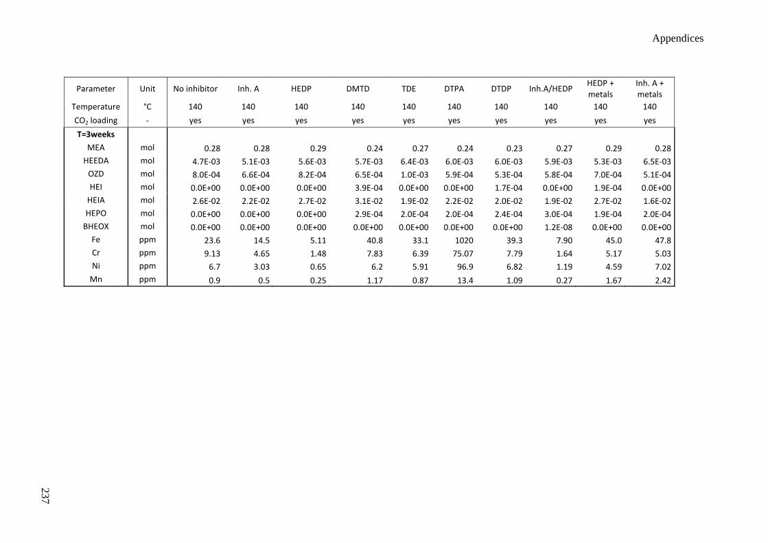
Appendices

237

Parameter Unit No inhibitor Inh. A HEDP DMTD TDE DTPA DTDP Inh.A/HEDP HEDP + metals

Inh. A + metals

Temperature °C 140 140 140 140 140 140 140 140 140 140

CO2 loading - yes yes yes yes yes yes yes yes yes yes

T=3weeks

MEA mol 0.28 0.28 0.29 0.24 0.27 0.24 0.23 0.27 0.29 0.28

HEEDA mol 4.7E-03 5.1E-03 5.6E-03 5.7E-03 6.4E-03 6.0E-03 6.0E-03 5.9E-03 5.3E-03 6.5E-03

OZD mol 8.0E-04 6.6E-04 8.2E-04 6.5E-04 1.0E-03 5.9E-04 5.3E-04 5.8E-04 7.0E-04 5.1E-04

HEI mol 0.0E+00 0.0E+00 0.0E+00 3.9E-04 0.0E+00 0.0E+00 1.7E-04 0.0E+00 1.9E-04 0.0E+00

HEIA mol 2.6E-02 2.2E-02 2.7E-02 3.1E-02 1.9E-02 2.2E-02 2.0E-02 1.9E-02 2.7E-02 1.6E-02

HEPO mol 0.0E+00 0.0E+00 0.0E+00 2.9E-04 2.0E-04 2.0E-04 2.4E-04 3.0E-04 1.9E-04 2.0E-04

BHEOX mol 0.0E+00 0.0E+00 0.0E+00 0.0E+00 0.0E+00 0.0E+00 0.0E+00 1.2E-08 0.0E+00 0.0E+00

Fe ppm 23.6 14.5 5.11 40.8 33.1 1020 39.3 7.90 45.0 47.8

Cr ppm 9.13 4.65 1.48 7.83 6.39 75.07 7.79 1.64 5.17 5.03

Ni ppm 6.7 3.03 0.65 6.2 5.91 96.9 6.82 1.19 4.59 7.02

Mn ppm 0.9 0.5 0.25 1.17 0.87 13.4 1.09 0.27 1.67 2.42

List of publications

238

List of publications

Publications and oral presentations

Léonard G., Toye D., Heyen G., Optimal conception of a post-combustion CO2 capture unit with

assessment of solvent degradation, submitted for publication in Energy Procedia, 2013.

Léonard G., Mogador Cabeza B., Belletante S., Toye D., Heyen G., Modeling amine solvent

degradation for post-combustion CO2 capture, submitted for publication in Récents Progrès en Génie

des Procédés, 2013.

Léonard G., Mogador Cabeza B., Belletante S., Heyen G., Dynamic modeling and control of a pilot

plant for post-combustion capture, accepted for publication in Computer Aided Chemical Engineering

Vol.31, 2013.

Léonard G., Toye D., Heyen G., 2012. Study of 2-ethanolamine degradation. Oral presentation at the

“First University of Texas Concerence on CO2 capture and Storage”, Austin, USA.

Léonard G., Heyen G., 2011. Optimisation du procédé de captage de CO2 dans des solvants aminés.

Oral presentation at the “XIIIème Congrès de la Société Française de Génie des Procédés”, Lille,

France.

Léonard G. and Heyen G., Optimization of the CO2 capture process in amine solvents, Récents

Progrès en Génie des Procédés Vol. 101, 2011.

Leonard G. and Heyen G., Modeling post-combustion CO2 capture with amine solvents, Computer

Aided Chemical Engineering Vol. 29, pp 1768-1772, 2011.

Léonard G., Heyen G., 2010. Modeling post-combustion CO2 capture with amine solvents. Oral

presentation at the “Computer Aided Process Engineering Forum”, Aachen, Germany.