Abstract—The purpose of this research is to optimal design

and control of heliostat for solar power generation in real time. Tracking the sun and calculating the position of the sun are possible by using illuminance sensor (CdS) and Simulink program. As heat transfer from heliostat to receiver is delivered by solar radiation, configuration factor commonly utilized in radiation is applied to control heliostat. Algorithms for maximizing configuration factor between sun, heliostat and receiver in real time are programmed by Simulink. By applying the optimized algorithms, the efficiency of the solar absorption in receiver can be maximized. Simulation was performed how to control azimuthal and elevation angles during the daytime with respect to diverse distances.

Index Terms—Configuration factor, heliostat, CdS, simulink, solar tracking device.

I. INTRODUCTION After the nuclear accident in Japan, renewable energy is

attracting attention nowadays. Among them, tower type solar thermal power system (STPS) has the high potential to replace conventional plant. STPS consists of hundreds of heliostats, receiver, storage and power cycle. Hundreds of heliostats reflect solar radiation to one receiver. Receiver temperature rises up to 500~1000oC. This generates high temperature steam or air which operates steam or gas turbine power generator. As the solar radiation from heliostat to receiver is depended on the angle and location of the heliostat, the algorithm of controlling the heliostat in real time is the most important factor to influence system efficiency and performance. [1-4] Therefore, this study was conducted to design and control of heliostat using a solar tracking device and a configuration factor commonly used in radiation heat transfer applications.

II. FUNDAMENTAL OPERATION OF SYSTEM

A. Configuration Factor The configuration factor commonly used in radiant heat

Manuscript received May 30, 2012; revised June 30, 2012. Dong Il Lee and Woo Jin Jeon are with the Propulsion and Combustion

Laboratory, School of Mechanical, Aerospace and System Engineering, Division of Aerospace Engineering, Korea Advanced Institute of Science and Technology (KAIST), 373-1 Guseong-dong, Yuseong-gu, Daejeon 305-701, Korea. Seung Wook Baek is with the Propulsion and Combustion Laboratory, School of Mechanical, Aerospace and System Engineering, Division of Aerospace Engineering, Korea Advanced Institute of Science and Technology (KAIST), 373-1 Guseong-dong, Yuseong-gu, Daejeon 305-701, Korea (e-mail: swbaek@kaist.ac.kr) Nazar T. Ali is with the Division of Electronic Engineering, Khalifa University of Science Technology and Research (KUSTAR), Sharjah 573, UAE.

transfer is changed by distance or angle between two surfaces. Consider two surfaces, 1 and 2, of an enclosure. Radiation from A1 to A2 can be described by Eq. 1. B1A1 is the total energy leaving the surface A1 as a constant and F1→2 indicates its fraction arriving at A2. So, radiation flux reaching the surface A2 is maximized when F1→2 is maximal. Eq. 2 is the definition of the configuration factor. Fig. 1(a) represents the fraction of total energy leaving surface 1 that is intercepted by surface 2.

(1)

(2)

(3)

Fig. 1. Schematic diagram of configuration factor.

Based on Eq. 2, Eq. 3 can be derived. In Eq. 3, Y is the multiplication of two configuration factors. Because the distance between the sun and heliostat and between the heliostat and receiver is constant, only the incidence angle is

Optimal Design and Control of Heliostat for Solar Power Generation

Dong Il Lee, Woo Jin Jeon, Seung Wook Baek,

1 2 1 1 1 2.q B A F→ →=

1 2

1 21 2 2 12

1

cos cos1 .A A

F dA dAA d

θ θπ− = ∫ ∫

1 2 2 3cos cos cos cos .Y θ θ θ θ=

IACSIT International Journal of Engineering and Technology, Vol. 4, No. 4, August 2012

388

and Nazar T. Ali

considered in Eq. 3. Fig. 1(b) is a schematic diagram of two configuration

factors. There are two assumptions. Firstly, θ1 is zero because of the large scale of sun. Secondly, the incident angle of radiation on receiver surface θ3 is predetermined by the position of the heliostat. Thus, the purpose of this research is to calculate each θ2 for each heliostat depending on the movement of the sun.

B. Calculation of Azimuthal and Elevation Angles for the Heliostat Fig. 1(b) also shows the azimuthal and elevation angles for

the sun and heliostat. Using this schematic, the equations below can be induced. According to Fig. 1(b), S indicates unit vector directed from heliostat center to sun in equation 4, while H means normal unit vector from heliostat surface as in equation 5. Finally, R represents unit vector directed from heliostat to receiver in equation 6. Equations 4, 5 and 6 can be derived by using polar coordinates as follows. [5]

(4)

(5)

(6)

(7)

(8)

Equation 7 represents the dot product between the unit vector directed from the heliostat center to the receiver and the unit vector directed from the heliostat center to the sun. Using the dot product, the reflection angle on the heliostat θ2 can be derived with Eq. 8.

(9)

(10)

(11)

(12)

(13)

(14)

Equation 9 also comes from Fig. 1(b) using the second law

of cosines. Using Equations 4, 5, and 9, Equations 10, 11, and 12 can be derived. Equations 13 and 14 represent the azimuthal and elevation angles of the heliostat, respectively.

These equations were programmed in Simulink, and a simulation was conducted during the daytime with respect to diverse distances.

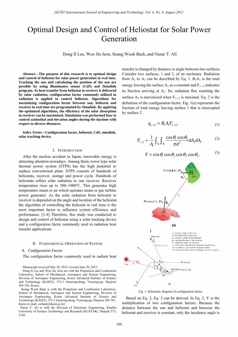
C. Overall Control System Fig. 2(a) shows overview of the control algorithm. Two

solar sensors for azimuthal angle and two solar sensors for elevation angle are used to set the sun position. A Simulink program calculates the elevation and azimuthal angles of the sun using signals received from these four solar sensors. After determining the location of the sun, the Simulink program calculates θ2 using equation 8 to determine the optimal configuration factor. The optimal angle of θ2 is then used to control the elevation and azimuthal angles of the heliostat using its two motors (one for elevation angle and the other for azimuthal angle). This optimized control algorithm enhances system efficiency.

Fig. 2. Control algorithm and schematic diagram of solar tracking device.

D. Solar tracking Device Fig. 2(b) shows a configuration of the solar tracking device,

which consists of a controller, two stepping motors, and four CdS sensors. The controller uses Simulink to calculate the sun position and operate the stepping motors. Stepping motors are commonly used in precision positioning control applications. The stepping motor used in the prototype has

S = cos sin cos cos sin .x y zS i S j S k e Ai e Aj ek+ + = + +

H = cos sin cos cos sin .x y z H H H H HH i H j H k e A i e A j e k+ + = + +

2 2 2

( ) ( ) ( )R = .( ) ( ) ( )

R H R H R Hx y z

R H R H R H

x x i y y j z z k R i R j R kx x y y z z

− + − + − = + +− + − + −

2cos(2 ) = R S = = cos sin cos cos sin .x x y y z z x y zRS RS RS R e A R e A R eθ + + + +

1

2

cos ( cos sin cos cos sin ) = .

2x y zR e Ai R e A R e

θ− + +

2 2

( ) ( ) ( ).

2cos 2cosx x y y z zR S i R S j R S kR SH

θ θ+ + + + ++= =

2

cos sinsin .2cos cos

xH

H

R e AAeθ

+=

2

cos coscos .

2cos cosy

HH

R e AA

eθ+

=

2

sinsin .2cos

zH

R eeθ

+=

tan 2(sin ,cos ).H H HA a A A=

1

2

sinsin ( ).2cosz

HR ee

θ− +=

IACSIT International Journal of Engineering and Technology, Vol. 4, No. 4, August 2012

389

specification of 24 V, 0.072o per step, and five phases. The voltage of the CdS sensor changes with the brightness of the light. Depending on the position of the sun, the cylindrical pillar has differing shadows. On the outside of the cylinder, north-, south-, east-, and west-facing CdS sensors detect the brightness of the ambient light. The voltage values, which vary with the brightness of the light, are inputted to an analog-to-digital converter. Mean voltage values (east–west and north–south) are set at a threshold value. When a CdS sensor provides a value lower than the threshold voltage, the system automatically adjusts the direction of azimuthal and elevation angle. Of the four CdS sensors (A, B, C, D), A and B are used to detect the azimuthal angle, while C and D to detect the elevation angle.

As the sun moves to the west, shadows are formed on the east side. The reduced light causes the voltage value of the east-side ambient CdS sensor to decrease relative to that of the ambient CdS sensor located on the west side. Thus, tracking the sun is performed by activating the motor to move the heliostat toward the west until the output voltage of two CdS sensors A and B (azimuthal) is equal. The cylindrical housing height is calculated as follows: h is the height of the cylindrical housing, d is the diameter of the CdS sensor, and the trigonometric formula is tan /h dθ = . If the angle of the shadow formed by the cylindrical pillar is within 1°, h can be obtained by tan1oh d= ⋅ .

If a CdS sensor (R1) and a resistor (R2) are connected to a circuit voltage, the output voltage can be calculated by the following expression: 2 / ( 2 1)out inV V R R R= ⋅ + When using this equation, output voltage increases in bright places because of the reduced resistance of R1 and decreases in dark places due to the increased resistance of R1. The output voltage is inputted to an analog-to-digital converter.

E. Several Simulink Algorithm When CdS sensors located on the east side and west side

detect voltage values, the average voltage of the two CdS sensors is calculated. This average value is set to a threshold value. If the voltage on the east side is lower than the threshold of the average azimuthal voltage and higher than a cloudy threshold, the condition causes the true value. If this condition is not satisfied, it generates a false value. The sensor value of the west side is calculated in the same way by a conditional statement. Also, solar tracking is stopped when the average threshold calculations per second (east–west, north–south) is lower than the cloudy threshold criterion. If the control signal for forward and reverse rotation is entered into the motor at the same time, the motor causes the step out. Thus, one of the signals should be sent to the motor. The control algorithm for clockwise and counterclockwise movement is the same as above for the elevation angle.

The procedure for calculating the azimuthal or elevation angle is as follows. Firstly, the number of pulses is calculated when the motor operates clockwise. Secondly, the clockwise angle is computed by multiplying the per pulse angle of the moving motor. Thirdly, the clockwise rotation angle is calculated by subtracting the counterclockwise angle. Finally, the azimuthal angle can be obtained by adding the initial azimuthal angle. The calculation algorithm for the elevation angle is the same as above.

III. RESULTS AND DISCUSSION This experimental azimuthal and elevation angle at the

Korea Advanced Institute of Science and Technology (KAIST) was compared with the actual value, obtained from Korea Astronomy and Space Science Institute (KASSI). The maximum error was within 1° between 8:00 am and 5:00 pm. According to these results, the algorithm used for the solar tracking device is correct.

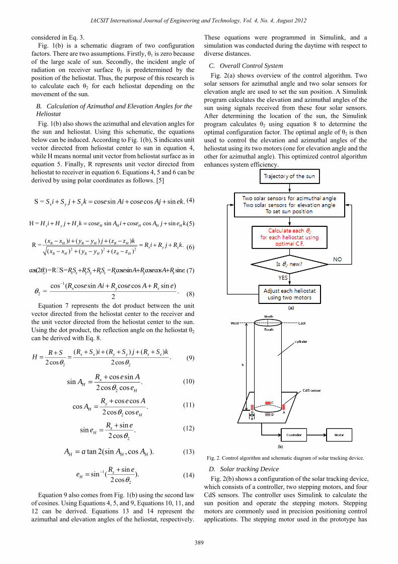
A. Experimental Verification of the Heliostat Experimental verification was carried out from 10 a.m. to 5

p.m. Solar tracking device and heliostat was operated by a programmed algorithm from east to west as shown in Fig. 3.

Fig. 3. Transient motion of heliostat by hour.

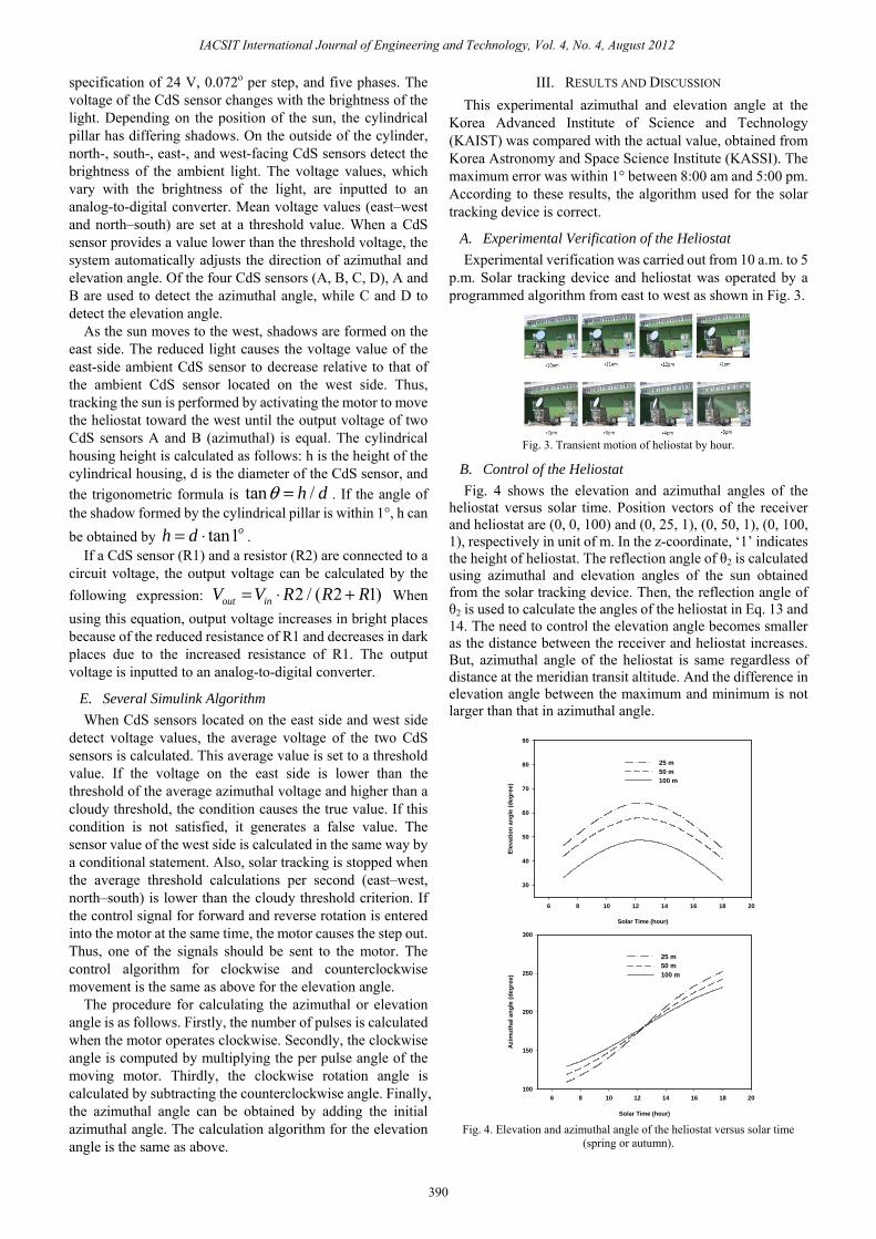
B. Control of the Heliostat Fig. 4 shows the elevation and azimuthal angles of the

heliostat versus solar time. Position vectors of the receiver and heliostat are (0, 0, 100) and (0, 25, 1), (0, 50, 1), (0, 100, 1), respectively in unit of m. In the z-coordinate, ‘1’ indicates the height of heliostat. The reflection angle of θ2 is calculated using azimuthal and elevation angles of the sun obtained from the solar tracking device. Then, the reflection angle of θ2 is used to calculate the angles of the heliostat in Eq. 13 and 14. The need to control the elevation angle becomes smaller as the distance between the receiver and heliostat increases. But, azimuthal angle of the heliostat is same regardless of distance at the meridian transit altitude. And the difference in elevation angle between the maximum and minimum is not larger than that in azimuthal angle.

Fig. 4. Elevation and azimuthal angle of the heliostat versus solar time (spring or autumn).

Solar Time (hour)

6 8 10 12 14 16 18 20

Elev

atio

n an

gle

(deg

ree)

30

40

50

60

70

80

90

25 m50 m100 m

Solar Time (hour)

6 8 10 12 14 16 18 20

Azi

mut

hal a

ngle

(deg

ree)

100

150

200

250

300

25 m50 m100 m

IACSIT International Journal of Engineering and Technology, Vol. 4, No. 4, August 2012

390

IV. CONCLUSIONS An optimized design and control of heliostat was

conducted using a solar tracking device and a configuration factor commonly used in radiation heat transfer applications. Comparison of the experimental results with KASSI mathematical data for sun position confirmed that the algorithm used for the solar tracking device was correct. A simulation for controlling elevation and azimuthal angle of the heliostat was conducted during the day with respect to differing distances. Dissimilar distances from the receiver to the heliostat show interesting results. As this distance gets larger, elevation angle gets smaller. Furthermore, azimuthal angle is the same at the meridian transit altitude regardless of the distance. Finally, design and applied control algorithms of heliostat were validated

ACKNOWLEDGEMENTS This work was supported by the “Human Resources

Development” of the Korea Institute of Energy Technology Evaluation and Planning (KETEP) grant funded by the Korea government Ministry of Knowledge Economy. (No. 20094010100050)

REFERENCES [1] S. A. Kalogirou, “Design and construction of a one-axis sun-tracking

system,” Solar Energy. 1996, vol. 57, no. 6, pp. 465-469. [2] P. Roth, A. Georgiev, and H. Boudinov, “Design and construction of a

system for sun-tracking,” Renewable Energy. 2004, vol. 29, pp. 393-402.

[3] H. Arbab, B. Jazi, and M. Rezagholizadeh, “A computer tracking system of solar dish with two-axis degree freedoms based on picture processing of bar shadow,” Renewable Energy. 2009, vol. 34, pp. 1114-1118.

[4] W. A. Lynch and Z. M. Salameh, “Simple electro-optically controlled dual-axis sun tracker,” Solar Energy. 1990, vol. 45, no. 2, pp. 65-69.

[5] Y. C. Park, “Heliostat control system,” Journal of the Korean Solar Energy Society. 2009, vol. 29, no. 1, pp. 50-57.

IACSIT International Journal of Engineering and Technology, Vol. 4, No. 4, August 2012

391