OPTIMAL DESIGN AND ANALYSIS OF CLONAL FORESTRY

OPTIMAL DESIGN AND ANALYSIS OF CLONAL FORESTRY

TRIALS USING SIMULATED DATA

By

SALVADOR ALEJANDRO GEZAN

A DISSERTATION PRESENTED TO THE GRADUATE SCHOOL OF THE UNIVERSITY OF FLORIDA IN PARTIAL FULFILLMENT

OF THE REQUIREMENTS FOR THE DEGREE OF DOCTOR OF PHILOSOPHY

UNIVERSITY OF FLORIDA

2005

Copyright 2005

by

Salvador Alejandro Gezan

"If a scientific heresy is ignored or denounced by the general public,

there is a chance it may be right. If a scientific heresy is emotionally supported by the general public,

it is almost certainly wrong." (Isaac Asimov, 1977)

Dedicated to: My biological family, Tita, Lincoln, Ivan, Demain, Florencia and Alexandra My political family, Dean, Quena and Becky, Lauren, Anha and Kevin And to an special individual that put us all together, Pincho

iv

ACKNOWLEDGMENTS

I would like to thank the members of my supervisory committee, Drs. T.L. White,

R.C. Littell, D.A. Huber, D. S. Wofford, and R. L. Wu, for their energy, time and help

during my program. I thank, in particular to Dr. White, for the opportunity to come to

Gainesville and do such an interesting project and also for his patience and wiliness to

show me not only science, but also emotional intelligence. I thank to Dr. Huber, for many

small but important details, and for showing me a different dimension of thinking,

sometimes unreachable but which surprisingly I liked. I thank to Dr. Littell, an

unconditional supporter and also model in many senses.

This research would not have been done without the financial support of the

members of the Cooperative Forest Genetic Research Program (CFGRP). Here, I want to

thank Greg Powell for his enormous support in several aspects, and for showing me what

being a gator is all about.

I also want to thank several friends: The Latino Mafia, Veronica, Alex, Rodrigo,

Bernardo, Belkys, Gabriela, and Rossanna; the Trigators Mafia, Terrence, Mathew,

Shannon, Josh, Betsy, Mark, and with special love Eugenia.

Special thanks go to all members of my family for tolerating my absence, but

particularly to my step father Dean W. Pettit, for his unusual vision and for opening doors

for me to cross as I choose.

v

TABLE OF CONTENTS page

ACKNOWLEDGMENTS ................................................................................................. iv

LIST OF TABLES............................................................................................................ vii

LIST OF FIGURES .............................................................................................................x

ABSTRACT..................................................................................................................... xiii

CHAPTER

1 INTRODUCTION ........................................................................................................1

2 COMPARISON OF EXPERIMENTAL DESIGNS FOR CLONAL FORESTRY USING SIMULATED DATA......................................................................................7

Introduction...................................................................................................................7 Materials and Methods ...............................................................................................10

Field Layout.........................................................................................................10 Genetic Structure and Linear Model ...................................................................12 Spatial Surface.....................................................................................................13 Simulation Process ..............................................................................................15 Simulating Mortality ...........................................................................................16 Statistical Analysis ..............................................................................................17

Results and Discussion ...............................................................................................19 Variance Components .........................................................................................19 Correlations between True and Predicted Clonal Values....................................22 Heritabilities for Simulated Designs ...................................................................24

Conclusions.................................................................................................................26

3 ACHIEVING HIGHER HERITABILITIES THROUGH IMPROVED DESIGN AND ANALYSIS OF CLONAL TRIALS.................................................................29

Introduction.................................................................................................................29 Materials and Methods ...............................................................................................31

Field Design and Simulation ...............................................................................31 Statistical Models ................................................................................................33

Results and Discussion ...............................................................................................36 Heritability Estimates and Confidence Intervals .................................................36

vi

Surface Parameter Behavior ................................................................................40 Latinization..........................................................................................................43 Number of Ramets per Clone ..............................................................................44

Conclusions and Recommendations ...........................................................................47

4 ACCOUNTING FOR SPATIAL VARIABILITY IN BREEDING TRIALS ...........49

Introduction.................................................................................................................49 Materials and Methods ...............................................................................................53

Field Design and Simulation ...............................................................................53 Statistical Analysis ..............................................................................................55

Results.........................................................................................................................59 Modeling Global and Local Trends.....................................................................59 Nearest Neighbor Models....................................................................................65

Discussion...................................................................................................................68 Modeling Global and Local Trends.....................................................................69 Nearest Neighbor Models....................................................................................72

Conclusions.................................................................................................................75

5 POST-HOC BLOCKING TO IMPROVE HERITABILITY AND BREEDING VALUE PREDICTION..............................................................................................77

Introduction.................................................................................................................77 Materials and Methods ...............................................................................................79 Results.........................................................................................................................83 Discussion...................................................................................................................88

6 CONCLUSIONS ........................................................................................................93

APPENDIX

A SUPPLEMENTAL TABLES .....................................................................................98

B EXTENSIONS IN CONFIDENCE INTERVALS FOR HERITABILITY ESTIMATES ............................................................................................................106

C MATLAB SOURCE CODE.....................................................................................108

Annotated Matlab Code to Generate Error Surfaces. ...............................................108 Annotated Matlab Code to Generate Clonal Trials. .................................................109

LIST OF REFERENCES.................................................................................................112

BIOGRAPHICAL SKETCH ...........................................................................................118

vii

LIST OF TABLES

Table page 2-1 Simulated designs and their number of replicates, blocks per replicate, plots per

block, and trees per block for single-tree plots (STP) and four-tree row plots (4-tree). The number of rows and columns is given for the row-column design. All designs contained 2,048 trees arranged in a rectangular grid of 64 x 32 positions..12

2-2 Linear models fitted for simulated datasets for single-tree plots (STP) and four-tree row plots (4-tree) over all surface patterns, plot and design types. All model effects were considered random. ..............................................................................18

3-1 Linear models fitted for non-Latinized experimental designs over all surface patterns. All model effects other than the mean were considered random. .............33

3-2 Linear models fitted for Latinized linear experimental designs over all surface patterns. All model effects other than the mean were considered random. .............33

3-3 Average individual single-site broad-sense heritability with its standard deviations in parenthesis and relative efficiencies calculated over completely randomized design for experimental designs and linear models that were not Latinized (No-LAT). Note that the parametric HB

2 was established for CR design as 0.25. ..........................................................................................................37

3-4 Coefficient of variation (100 std /⎯x) for the estimated variance component for clone and error on 3 surface patterns, different number of ramets per clone and 3 selected experimental designs. .................................................................................45

4-1 Linear models fitted for simulated datasets using classical experimental designs to model global trends: complete randomized (CR), randomized complete block (RCB), incomplete block design with 32 blocks (IB), and row-column (R-C) design. All model effects other than the mean were considered random.................56

4-2 Linear models fitted for simulated datasets using polynomial functions to model global trends: linear (Linear), quadratic (Red-Poly), and quadratic model with some interactions (Full-Poly). All variables are assumed fixed and the treatment effect is random. .......................................................................................................56

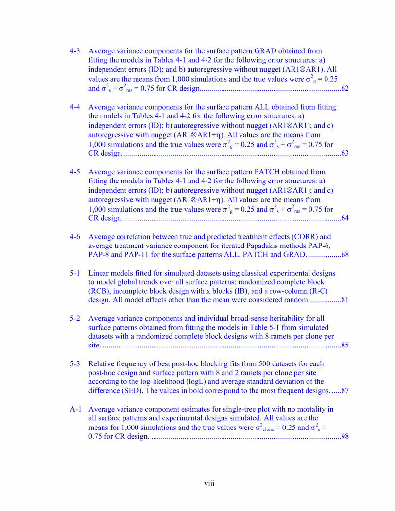
viii

4-3 Average variance components for the surface pattern GRAD obtained from fitting the models in Tables 4-1 and 4-2 for the following error structures: a) independent errors (ID); and b) autoregressive without nugget (AR1⊗AR1). All values are the means from 1,000 simulations and the true values were σ2

g = 0.25 and σ2

s + σ2ms = 0.75 for CR design.........................................................................62

4-4 Average variance components for the surface pattern ALL obtained from fitting the models in Tables 4-1 and 4-2 for the following error structures: a) independent errors (ID); b) autoregressive without nugget (AR1⊗AR1); and c) autoregressive with nugget (AR1⊗AR1+η). All values are the means from 1,000 simulations and the true values were σ2

g = 0.25 and σ2s + σ2

ms = 0.75 for CR design. ................................................................................................................63

4-5 Average variance components for the surface pattern PATCH obtained from fitting the models in Tables 4-1 and 4-2 for the following error structures: a) independent errors (ID); b) autoregressive without nugget (AR1⊗AR1); and c) autoregressive with nugget (AR1⊗AR1+η). All values are the means from 1,000 simulations and the true values were σ2

g = 0.25 and σ2s + σ2

ms = 0.75 for CR design. ................................................................................................................64

4-6 Average correlation between true and predicted treatment effects (CORR) and average treatment variance component for iterated Papadakis methods PAP-6, PAP-8 and PAP-11 for the surface patterns ALL, PATCH and GRAD. .................68

5-1 Linear models fitted for simulated datasets using classical experimental designs to model global trends over all surface patterns: randomized complete block (RCB), incomplete block design with x blocks (IB), and a row-column (R-C) design. All model effects other than the mean were considered random.................81

5-2 Average variance components and individual broad-sense heritability for all surface patterns obtained from fitting the models in Table 5-1 from simulated datasets with a randomized complete block designs with 8 ramets per clone per site. ...........................................................................................................................85

5-3 Relative frequency of best post-hoc blocking fits from 500 datasets for each post-hoc design and surface pattern with 8 and 2 ramets per clone per site according to the log-likelihood (logL) and average standard deviation of the difference (SED). The values in bold correspond to the most frequent designs. .....87

A-1 Average variance component estimates for single-tree plot with no mortality in all surface patterns and experimental designs simulated. All values are the means for 1,000 simulations and the true values were σ2

clone = 0.25 and σ2ε =

0.75 for CR design. ..................................................................................................98

ix

A-2 Average variance component estimates for four-tree plot with no mortality in all surface patterns and experimental designs simulated. All values are the means for 1,000 simulations and the true values were σ2

clone = 0.25 and σ2ε = 0.75 for

CR design. ................................................................................................................99

A-3 Average variance component estimates for single-tree plot with 25% mortality in all surface patterns and experimental designs simulated. All values are the means for 1,000 simulations and the true values were σ2


0.75 for CR design. ................................................................................................100

A-4 Average variance component estimates for four-tree plot with 25% mortality in all surface patterns and experimental designs simulated. All values are the means for 1,000 simulations and the true values were σ2


0.75 for CR design. ................................................................................................101

A-5 Average estimated correlations between true and predicted clonal (CORR) with standard deviations for 0 and 25% mortality obtained from 1,000 simulations for single-tree plots (STP) and four-tree plot row plots (4-tree) in all surface patterns and experimental designs. ......................................................................................102

A-6 Average individual broad-sense heritability calculated for single-tree plot (STP) and four-tree plot (4-tree) with their standard deviations in all surface patterns, experimental designs and mortality cases. All values are the means for 1,000 simulations and the base heritability value was 0.25 for CR design......................103

A-7 Coefficient of variation (100 std /⎯x) for broad-sense individual heritability obtained from 1,000 simulations with 8 ramets per clone for single-tree plot in all surface patterns and experimental designs. .......................................................104

A-8 Average correlations between true and predicted treatment effects (CORR) with standard deviations in parenthesis in the ALL surface patterns for 2 and 8 ramets per clone for selected experimental designs analyses and polynomial models fitted for the following error structures: independent errors (ID); autoregressive without nugget (AR1⊗AR1); and autoregressive with nugget (AR1⊗AR1+η). ..105

A-9 Original and post-hoc blocking average individual broad-sense heritabilities with standard deviations in parenthesis for all surface patterns obtained from fitting the models in Table 5-1 from simulated datasets with a randomized complete block design with 8 ramets per clone per site.........................................105

x

LIST OF FIGURES

Figure page 2-1 Replicate layout for randomized complete block design simulations for single-

tree plots (left) and four-tree row plots (right). The same 8 resolvable replicates were used for incomplete block and row-column designs. All simulations had 256 unrelated clones with 8 ramets per clone for a total of 2,048 trees...................11

2-2 Average proportions of restricted maximum likelihood (REML) variance component estimates (after correction so that all components sum to one) for single-tree and four-tree row plots for the no mortality case in all surface patterns and experimental designs simulated. ..........................................................21

2-3 Average estimated correlations between true and predicted clonal values (CORR) obtained from 1,000 simulations for single-tree and four-tree row plots in the 0% mortality case for all surface patterns and designs. .................................23

2-4 Average heritabilities obtained for single-tree and four-tree row plots in each surface pattern and design type for the no mortality case. The error bars correspond to the upper limit for a 95% confidence interval of the mean. ..............25

2-5 Heritability distributions for the no mortality case in the surface pattern ALL for selected completely randomized (CR), randomized complete block (RCB), and row-column (R-C) designs in single-tree and four-tree row plots. ..........................25

3-1 Plots of means and 95% confidence intervals for estimated individual broad-sense heritabilities obtained from simulation runs and by the method proposed by Dickerson (1969) for all design types and surface patterns for non-Latinized designs and analyses (No-LAT). Average heritabilities correspond to the central points in each confidence interval, and all simulations involved 8 ramets per clone. ........................................................................................................................38

3-2 Contours for individual heritabilities obtained by using the lowess smoother (Cleveland 1979) of row-column design for different surface parameters from fitting experimental designs and analyses that were non-Latinized (No-LAT). ......39

3-3 Average individual heritability estimates for ALL and PATCH surface pattern for simulated surfaces for subsets of simulations with High (ρx > 0.7 and ρy > 0.7) and Low (ρx < 0.3 and ρy < 0.3) spatial correlations.........................................42

xi

3-4 Distribution of individual broad-sense heritability estimates for row-column designs with 2 and 8 ramets per clone obtained from 500 simulations each for the surface patterns ALL and PATCH from fitting experimental designs and analyses that were non-Latinized (No-LAT). ..........................................................46

3-5 Average values for row-columns design in all surface patterns from fitting experimental designs and analyses that were non-Latinized: a) Clonal mean heritabilities (the whiskers correspond to the 95% confidence intervals); and b) Clonal mean heritability increments. .......................................................................46

4-1 Neighbor plots and definitions of covariates used in Papadakis (PAP) and Moving Average (MA) methods. Plots with the same numbers indicate a common covariate. ...................................................................................................58

4-2 Average correlations between true and predicted treatment effects (CORR) in 3 different surface patterns for classical experimental design analyses and polynomial models fitted for the following error structures: independent errors (ID); autoregressive without nugget (AR1⊗AR1); and autoregressive with nugget (AR1⊗AR1+η). Surface GRAD is not shown in the last graph because few simulations converged.......................................................................................61

4-3 Average correlations between true and predicted treatment effects (CORR) in 3 different surface patterns for nearest neighbor analyses fitted assuming independent errors. PAP: Papadakis, MA: Moving Average...................................67

4-4 Average correlations between true and predicted treatment effects (CORR) in 3 different surface patterns for selected methods: randomized complete block (RCB), row-column (R-C), and Papadakis (PAP) using the following error structures: independent errors (ID), and autoregressive with nugget (AR1⊗AR1+η). .......................................................................................................67

5-1 Experimental layout for randomized complete block design simulations with 8 resolvable replicates (left) and partitioning of one replicate for incomplete block design layouts (right). All simulations had 256 unrelated clones with 8 ramets per clone per site for a total of 2,048 trees. ..............................................................81

5-2 Average correlation between true and predicted clonal values (CORR) for original and post-hoc bloking analyses on ALL, PATCH and GRAD surface patterns for simulated surfaces with 8 ramets per clone. .........................................84

5-3 Average individual heritability (a) and correlation between true and predicted clonal values (b) calculated over 500 simulations with a randomized complete block designs with 8 ramets per clone per site for each surface pattern and post-hoc design.................................................................................................................86

xii

5-4 Average correlation between true and predicted clonal values (CORR) calculated for ALL and PATCH surface patterns and all post-hoc designs for sets with High (ρx, > 0.7 and ρy > 0.7) and Low (ρx < 0.3 and ρy < 0.3) spatial correlations. The datasets used corresponded to simulated surfaces with a randomized complete block design and 8 ramets per clone per site. .......................89

B-1 Plots of means and 95% confidence intervals for broad-sense heritabilities for single-tree plots (STP) and four-tree row plots (4-tree) in all designs and surface patterns for non-Latinized designs and analyses (No-LAT) with 25% mortality. The methods correspond to simulation runs and the approximation proposed by Dickerson (1969). Average heritabilities correspond to the central points in each confidence interval. ................................................................................................107

xiii

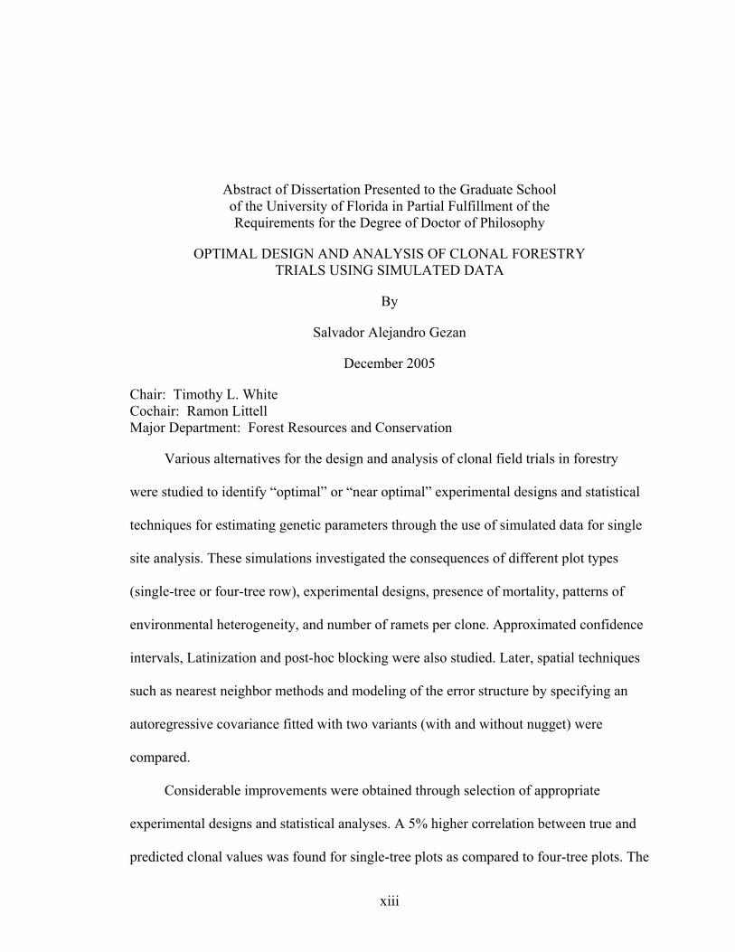
Abstract of Dissertation Presented to the Graduate School of the University of Florida in Partial Fulfillment of the Requirements for the Degree of Doctor of Philosophy

OPTIMAL DESIGN AND ANALYSIS OF CLONAL FORESTRY TRIALS USING SIMULATED DATA

By

Salvador Alejandro Gezan

December 2005

Chair: Timothy L. White Cochair: Ramon Littell Major Department: Forest Resources and Conservation

Various alternatives for the design and analysis of clonal field trials in forestry

were studied to identify “optimal” or “near optimal” experimental designs and statistical

techniques for estimating genetic parameters through the use of simulated data for single

site analysis. These simulations investigated the consequences of different plot types

(single-tree or four-tree row), experimental designs, presence of mortality, patterns of

environmental heterogeneity, and number of ramets per clone. Approximated confidence

intervals, Latinization and post-hoc blocking were also studied. Later, spatial techniques

such as nearest neighbor methods and modeling of the error structure by specifying an

autoregressive covariance fitted with two variants (with and without nugget) were

compared.

Considerable improvements were obtained through selection of appropriate

experimental designs and statistical analyses. A 5% higher correlation between true and

predicted clonal values was found for single-tree plots as compared to four-tree plots. The

xiv

best experimental designs were row-column for single-tree plots, and incomplete blocks

with 32 blocks for four-tree row plots increasing heritability by 10% and 14% over a

randomized complete block design, respectively. Larger variability of some variance

component estimates was the only effect of 25% mortality. Experiments with more

ramets per clone yielded higher clonal mean heritabilities, and using between 4 and 6

ramets per clone per site is recommended.

Dickerson’s approximate method for estimating the variance of heritability

estimates produced reasonable 95% confidence intervals, but an underestimation was

detected in the upper confidence limit of complex designs. The effects of implementing

Latinization were significant for increasing heritability, but small in practical terms. Also,

substantial improvements in statistical efficiency were obtained using post-hoc blocking,

with negligible differences compared to pre-designed local control with no reduction in

the genetic variance as the size of the block decreased.

For spatial analyses, the incorporation of a separable autoregressive error structure

with or without nugget yielded the best results. Differences between experimental designs

were almost non-existent when an error structure was also modeled. Some variants of the

Papadakis method were almost as good as models that incorporated the error structure.

Further, an iterated Papadakis method did not produce improvements over the non-

iterated Papadakis.

1

CHAPTER 1 INTRODUCTION

Genetic testing is a critical activity for all breeding programs; however, it is time-

consuming and frequently one of the most expensive processes (Zobel and Talbert 1984,

p. 232). Appropriate selection of experimental design and statistical analysis can yield

considerable improvements in terms of increased precision of genetic parameter estimates

and efficient use of resources. Genetic testing aims to achieve several objectives such as

(White 2004) 1) improved genetic gain from selection by evaluation of genetic quality; 2)

estimation of genetic parameters; 3) creation of a base population for future selection

cycles; and 4) quantification of realized genetic gains. Also, various operational decisions

depend on information obtained from genetic tests, and limited quantitative genetic

knowledge degrades the efficiency of a breeding program, eventually affecting potential

gains.

At present, there is extensive research in genetic testing for agricultural crops that

can be useful for testing in forestry; nevertheless, for forest species several important

differences must be considered. Forest sites tend to be heterogeneous, the individuals of

interest (trees) are usually large, and the screening of hundreds or thousands of genetic

entities (e.g., families or clones) is common. These elements imply the need for relatively

large test sites or the use of fewer replicates per site for each entry. Finding optimal

testing sites is difficult, and if areas with high environmental heterogeneity are selected,

the residual error variance will be inflated due to the confounding of tree-to-tree variation

with other large-scale environmental effects. Nevertheless, optimization of genetic testing

2

is possible in any of the following stages: 1) design of experiments; 2) implementation;

and 3) statistical analysis.

The design of experiments is a critical element and no single design will suit all

testing objectives and environmental conditions perfectly, but statistical and

computational tools are available to improve efficiency and they should be used as

safeguards against site heterogeneity or potential undetected biases. Traditionally, in

forest tree improvement, randomized complete block designs have been the design of

choice, which is effective when within replicate (or block) variability is relatively small,

a situation that is rare in forest sites (Costa e Silva et al. 2001). Nevertheless, more

complex and efficient designs can be easily implemented. Incomplete block designs

allow for a better control of site heterogeneity by specifying smaller compartments than

do randomized complete block design. Also, row and column positions of the

experimental units can be utilized to simultaneously implement two-way blocking factors

producing row-column designs. Other design options include the utilization of restricted

randomization such as Latinization, nested structures and spatial designs (Whitaker et al.

2002).

In the second stage of optimizing experimental precision (i.e., implementation), it is

important to exercise control at all levels of field testing (installation, maintenance and

measurement) with proper care on documentation, labeling, randomization, site

uniformity and survival. The objectives of this stage are to control for all possible factors

that might increase experimental noise, and, therefore, reduce precision of estimation of

parameters of interest.

3

The stage of statistical analysis is also very important. The use of mixed linear

models combined with techniques such as restricted maximum likelihood (REML) to

estimate variance components and to predict random effects is well understood and

broadly used. Spatial analysis (Gilmour et al. 1997) and nearest neighbor methods

(Vollmann et al. 1996) are interesting techniques used to improve prediction of genetic

values. Spatial analyses are particularly attractive because they incorporate the

coordinates of the experimental units (plots, trees or plants) in the linear model to account

for physical proximity by modeling the error structure (i.e., environmental heterogeneity).

Another relevant tool is post-hoc blocking, which consists of superimposing complete or

incomplete blocks over the original field design and fitting a modified linear model as if

the blocking effects were present in the original design.

Clonal forestry is a new practice in many widely used commercial forestry species,

e.g., Pinus spp., Eucalyptus spp. and Populus spp. (Carson 1986; Elridge et al. 1994, p.

230; Ritchie 1992). Clonal forestry refers to the use of a relatively small number of tested

clones deployed in operational plantations through mass-propagation techniques (Bonga

and Park 2003). Testing clones is of particular interest because the use of identical

genetic entities (ramets from a clone) allows sampling several environmental microsites,

thus allowing complete separation of genetic and environmental effects to increase the

precision of prediction of breeding values (Shaw and Hood 1985). Other benefits of

clonal testing include 1) achieving greater genetic gains than under traditional tree

breeding; 2) capturing greater portions of non-additive genetic variation for deployment;

3) using genotype x environment interaction by selecting clones most suited to specific

site conditions; 4) detecting and utilizing correlation breakers for traits with undesirable

4

genetic correlations; 5) preventing inbreeding in populations; 6) increasing plantation and

product uniformity; and 7) reducing time between breeding and testing cycles (Libby

1977; Libby and Rauter 1984; Zobel and Talbert 1984, p. 311).

There is extensive research relative to field testing of progenies using seedling from

half or full-sib families (e.g., White 2004). Some of these guidelines can be used for

clonal testing, but differences must be taken into consideration. In the literature, few

studies exist that give important guidelines for the design and analysis of clonal

experiments. The characteristics of the optimal designs and analyses are influenced by

many factors such as magnitudes of heritability, g x e interaction, and ratio of additive to

non-additive genetic variance. Also, several questions of interest remain to be answered.

For example, for the design of experiments: 1) are single-tree plots more efficient than

multiple-tree plots? is there an optimal incomplete block size? 2) how much better than

randomized complete blocks are incomplete blocks or row-column designs? 3) what are

the effects of mortality on the estimation of genetic parameters? 4) do the best designs

depend on the pattern of environmental heterogeneity? and 5) what is the optimal number

of ramets per clone?

For statistical analysis we require answers to the following: 1) is there any gain

from incorporating the error structure in the model? 2) is it necessary to model gradients?

3) how good are the nearest neighbor methods compared with spatial analysis

techniques? and 4) is post-hoc blocking useful; and how should we implement post-hoc

blocking?

One of the best ways to answer many of the above questions is with the use of

simulation techniques. Statistical simulation or Monte Carlo experiments are widely used

5

in statistical research. These methods are based on the generation of random numbers

with a computer to obtain approximate solutions to problems that are difficult to solve

analytically, and they can aid understanding and knowledge of the properties of the

experiments or methods of interest (Johnson 1987, p. 1). Particularly, for field testing,

they allow several alternatives to be evaluated without incurring large expense or having

to wait years before practical results are available.

The overall goal of this research was to identify “optimal” or “near optimal”

experimental designs and statistical analysis techniques for the prediction of clonal values

and estimation of genetic parameters in order to achieve maximum genetic gains from

clonal testing. This study explored single-site simulations with sets of unrelated clones

“planted” in environments with different patterns of variability.

In the first two chapters many alternative designs for clonal experiments are

compared. In Chapter 2, the consequences for the estimation of genetic parameters of

different design alternatives were studied. The elements compared were 1) single-tree

plot versus four-tree row plots; 2) several experimental designs; 3) no mortality versus

25% mortality; and 4) three different environmental patterns. For Chapter 3, more

detailed work was done with STP experiments. Here, individual heritabilities estimates

were examined in detail according to the different parameters used to simulate the

environmental patterns. Also, confidence intervals for heritability obtained using the

method proposed by Dickerson (1969) were compared with simulated percentile

confidence sets; and the effects of using different number of ramets per clone were

investigated.

6

Several statistical analysis techniques were studied in the last two chapters using

single-tree plot experiments only. First, in Chapter 4, multiple statistical tools were used

to account for spatial variability. The selected techniques included 1) modeling of global

trends through the use of traditional experimental designs or polynomial models; 2)

specification of a separable autoregressive error structure (with and without nugget); and

3) variants of nearest neighbor methods (Papadakis and Moving Average). Finally,

Chapter 5 aimed to understand consequences of and to define strategies for post-hoc

blocking. Some of the aspects evaluated included comparing performance of original

blocking versus post-hoc blocking for several experimental designs; and defining

strategies to select an optimal blocking structure within post-hoc blocking.

7

CHAPTER 2 COMPARISON OF EXPERIMENTAL DESIGNS FOR CLONAL FORESTRY USING SIMULATED DATA

Introduction

Genetic field tests of forest trees are critical to tree improvement serving to

estimate genetic parameters and evaluate provenances, families, and individuals. Genetic

testing of forest trees is a time-consuming process and is frequently the most expensive

activity of an improvement program (Zobel and Talbert 1984, p. 232). Therefore, it is of

primary interest to maximize benefits by allocating resources efficiently (Namkoong

1979, p. 117). It is common in forestry trials to study the performance of a large number

of genetic entries (e.g., families or clones), and this implies the need for relatively large

test sites or the use of fewer replicates per site for each entry. Because forest sites for

field experiments are often inherently variable, it is difficult to find optimal sites. The

presence of this environmental heterogeneity inflates the residual variance due to the

confounding of tree-to-tree variation with other, larger-scale environmental effects; and,

hence, decreases the benefits of using simple experimental designs (Grondona et al.

1996).

Within-site variability is caused by variation in natural factors such as soil,

microclimate, topography, wind and aspect. In addition other forms of heterogeneity

might originate from machinery, stock quality or planting technique. Some conditions

produced by topography or moisture might be easy to identify but, more commonly,

environmental heterogeneity is only recognized after the fact as differential response to

8

environmental conditions. Gradients across the site, local patches, and random microsite

variance are the common types of variability, and these sources may appear individually

or in combination (Costa e Silva et al. 2001), with some sources more frequent in

particular geographical areas.

There are three stages during which optimization of genetic testing can occur: 1)

experimental design and planning; 2) implementation; and 3) statistical analysis. Forest

genetic trials have traditionally employed randomized complete block designs (RCB) or,

more recently, incomplete block designs (IB). The RCB is most effective when the site is

relatively uniform within replicates, which is rarely the case in forest sites (Costa e Silva

et al. 2001). Reducing the size of the unit by incorporating incomplete blocks within a

full replicate (IB designs) allows for better control of site heterogeneity because smaller

blocks tend to be less variable than larger ones; therefore, IB designs have the potential to

increase precision over RCB (Cochran and Cox 1957, p. 386; Williams et al. 2002, p.

120). For simulated forest genetic trials under several environmental conditions, Fu et al.

(1998) report a 42% increase in the efficiency for IB over RCB. In a related study Fu et

al. (1999a) found that most of the within-site variation can be controlled using 5 to 20

plots per incomplete block with better results in those cases where square blocks were

employed instead of row or column blocks.

Another experimental option is the row-column design (John and Williams 1995, p.

87). When the experimental units are located in two-dimensional arrays, it is possible to

simultaneously implement two blocking factors (instead of one as in IB) corresponding to

the rows and columns of the experiment. Greater efficiencies are expected when row-

column designs are used (Lin et al. 1993; Williams and John 1996). Qiao et al. (2000),

9

using several wheat breeding trials, reported an increase of efficiency over RCB of 11%

for row-column designs compared with 8% for IB.

Clonal forestry is a new practice in many widely planted commercial tree species,

e.g., Pinus spp., Eucalyptus spp., Populus spp. (Carson 1986; Elridge et al. 1993, p. 230;

Ritchie 1992). Interest in clonal forestry stems from its additional benefits such as ability

to achieve greater genetic gains; potential to capture greater portions of non-additive

genetic variation and genotype x environment interaction; increased plantation and

product uniformity; and accelerated use of results from tree improvement by reducing

breeding and testing cycles (Libby 1977; Zobel and Talbert 1984, p. 311).

In the agronomy and forestry literature, there are several studies that compare

design and analysis alternatives for breeding experiments through real or simulated

datasets. In forest genetics, the few simulation studies available report some guidelines

for future testing. Fu et al. (1998) showed that α-designs were the most efficient

arrangement for IB designs. For the majority of the environmental conditions studied

they were superior to an RCB design for the estimation of family means, but the benefits

of IB over RCB were reduced as the level of missing observations increased (Fu et al.

1999b). In a related study for α-designs, Fu et al. (1999a) reported that smaller

incomplete blocks were more efficient for significant patches when single-tree plots were

established to estimate family and clonal means.

These studies give important guidelines for the design of genetic experiments;

nevertheless, several questions of interest remain to be answered: Are single-tree plots

more efficient than multiple-tree plots? In relation to IB designs, how much better (or

worse) are row-column designs? Is there an optimal incomplete block size? How is the

10

phenotypic variance partitioned under different experimental designs? Also, it is common

in previous simulation studies to screen a limited number of clones and to treat the

genetic entries as fixed effects in the linear model. In this study genetic entries were

assumed to be random, allowing estimation of heritabilities and prediction of clonal

genetic values for a range of simulated conditions.

The present study is focused on identifying “optimal” or “near optimal”

experimental designs for estimating genetic parameters and achieving maximum genetic

gain from forestry clonal tests. This study explores sets of unrelated clones tested on a

single site through the use of simulated data created with different patterns of

environmental variability. In particular, the objectives of these simulations are to

investigate the consequences for the estimation of genetic parameters of 1) using single-

tree or four-tree row plots; 2) using completely randomized, randomized complete block,

incomplete blocks of various sizes, or row-column designs; 3) experiencing no mortality

versus 25% mortality; and 4) planting on sites with different environmental patterns of

surface variation (only patches, only gradients, and both patches and gradients).

Materials and Methods

Field Layout

All simulations were based on a single trial of 2,048 trees planted on a contiguous

rectangular site of 64 rows and 32 columns with square spacing and 8 ramets for each of

the 256 unrelated clones. The trees were “planted” in either single-tree plots (STP) or

four-tree row plots (4-tree), corresponding to 8 and 2 plots per clone, respectively (Figure

2-1). A completely randomized design (CR) in which clonal plots were randomly

assigned to the field site was considered the baseline experimental design for each plot

size. A randomized complete block design (RCB), a variety of incomplete block designs

11

(IB), and a row-column design (R-C) were also implemented for both STP and 4-tree row

plots (Table 2-1).

There are many ways in which treatments (or clones in this case) can be allocated

to incomplete blocks. For the present work, α-designs were used to obtain IB and R-C

layouts. These designs can be obtained quickly and efficiently for many design

parameters (Williams et al. 1999). All IB and R-C designs were generated using the

software CycDesigN (Whitaker et al. 2002) that incorporates an algorithm to generate

optimal or near-optimal α-designs. Outputs from 100 different independent runs were

used for each design and plot type. CR and RCB layouts were generated using code

programmed in MATLAB (MathWorks 2000).

Figure 2-1. Replicate layout for randomized complete block design simulations for single-tree plots (left) and four-tree row plots (right). The same 8 resolvable replicates were used for incomplete block and row-column designs. All simulations had 256 unrelated clones with 8 ramets per clone for a total of 2,048 trees.

12

Table 2-1. Simulated designs and their number of replicates, blocks per replicate, plots per block, and trees per block for single-tree plots (STP) and four-tree row plots (4-tree). The number of rows and columns is given for the row-column design. All designs contained 2,048 trees arranged in a rectangular grid of 64 x 32 positions.

STP

Design a Replicates Blocks / Rep b Plots / Block Trees / Block

CR 1 1 2048 2048

RCB 8 1 256 256

IB 4 8 4 64 64

IB 8 8 8 32 32

IB 16 8 16 16 16

IB 32 8 32 8 8

R-C 8 32 rows 32 columns -

4-tree

Design Replicates Blocks / Rep Plots / Block Trees / Block

CR 1 1 512 2048

RCB 2 1 256 1024

IB 4 2 4 64 256

IB 8 2 8 32 128

IB 16 2 16 16 64

IB 32 2 32 8 32

R-C 2 16 rows 16 columns - a CR, complete randomized; RCB, randomized complete block; IB x, incomplete block with x blocks per

replicate; R-C, row-column. b Rep, resolvable replicate.

Genetic Structure and Linear Model

The linear model used to generate the simulated data was

)()( ijkmsijkskijk EECy +++= µ 2-1

where yijk is the response of the tree located in the ith row and jth column of the kth clone,

µ is a fixed population mean which was set equal to 10 units, Ck is the random genetic

clonal effect, Es(ijk) is the surface error (or structured residual) and Ems(ijk) corresponds to

the microsite random error (or unstructured residual).

13

The total variance for the above linear model (Equation 2-1) considering all

components as random is σ2T = σ2

clone + σ2s + σ2

ms. For simplicity, but without loss of

generality, σ2T was fixed to 1. Further, the variance structure for all surfaces and designs

was set to σ2clone = 0.25 and σ2

s + σ2ms = 0.75; hence, the single-site biased broad-sense

heritability HB2 = σ2

clone / (σ2clone + σ2

s + σ2ms) is 0.25 for completely randomized designs.

Spatial Surface

The spatial surface is a rectangular grid (x and y coordinates) composed of

unstructured and structured residuals. The unstructured errors, Ems, correspond to white

noise and can originate from measurement errors, planting technique, stock quality, and

unstructured microsite variation. The structured residuals, Es, are due to the underlying

environmental surface, and were generated from two distinct patterns: gradients and

patches. Gradients were modeled as a mean response vector t of size 2,048 x 1, at each of

the positions of the 64 x 32 grid, employing the following polynomial function:

)()( 22cicicicicicii yxyxyxt +++= βα 2-2

where xci and yci correspond to the centered values xci = xi –⎯x and yci = yi –⎯y for the ith

tree located in column x and row y; and α and β represent fixed weights on linear and

quadratic components, respectively. This function defines a flat plane (i.e., no gradients),

when α and β are zero. Also, the primary environmental gradient was oriented along the

short axis of the 64 x 32 rectangle to minimize variation within a replicate, as an

experiment would be laid out in the field.

Patches were modeled by incorporating a covariance structure based on a first-

order separable autoregressive process (AR1⊗AR1), which is a variant of the exponential

model used in spatial statistics (Littell et al. 1996, p. 305). This error structure has been

14

previously used successfully for analyses of agricultural experiments (Cullis and Gleeson

1991; Zimmerman and Harville 1991; Grondona et al. 1996; Gilmour et al. 1997) and

forestry trials (Costa e Silva et al. 2001; Dutkowsky et al. 2002). The AR1⊗AR1 error

structure considers two perpendicular correlations, one for the x direction (ρx) and the

other for y (ρy). The model defines an anisotropic model, where the covariance (or

correlation) between two observations is not only a function of their distance, but also of

their direction (Cressie 1993, p. 62). The parameters ρx and ρy define the correlation

between the structured residuals (Es) of nearby trees, and there is a positive relationship

between the magnitude of these parameters and patch size.

To generate the patches, a 2,048 x 2,048 variance-covariance matrix (R) was

constructed and later used to simulate residuals. The elements of this matrix were

obtained as

sieVar 2)( σ= for diagonal elements 2-3

hyy

hxxsii eeCov ρρσ 2

' ),( = for off-diagonal elements 2-4

where hx = | xi - xi’ |, hy = | yi - yi’ |, i.e., the absolute distance in row and column position

respectively, between two trees. The other parameters were previously defined.

This covariance structure also includes a nugget parameter (σ2ms), which allows the

modeling of discontinuities in covariance over very small distances. In real datasets the

nugget effect reflects variability that would be found if multiple measurements were

made exactly on the same position or the microsite variation of positions very close

together (Cressie 1993, p. 59; Young and Young 1998, p. 256).

15

Simulation Process

The first stage of the simulation consisted of the independent generation of surfaces

over which different experimental designs were superimposed. Each surface or

environmental pattern was produced by selecting 5 parameters at random from uniform

distributions (α, β, ρx, ρy and σ2ms). The parameters were restricted to the following

ranges: 0 to 0.05 for α, 0 to 0.0005 for β, 0.01 to 0.99 for the correlation parameters ρx

and ρy, and 0.15 to 0.60 for σ2ms. Additionally, these correlations were restricted so their

absolute difference was smaller than 0.85; and σ2s was calculated from σ2

s = 0.75 – σ2ms.

All these parameters were then used to generate the vector t and the residual

variance-covariance matrix R. The Cholesky decomposition of the R matrix was obtained

and used together with t and an independent random vector of standard normal numbers

to obtain the correlated residuals (Johnson 1987, p. 52-54), producing e ~ N(t, R). Later,

a set of normal independent random residuals was incorporated to constitute the white

noise (i.e., Ems). After this, all components were added together and a standardization was

performed to ensure that the total environmental variance was fixed at 0.75.

The remaining variability (0.25) belongs to the clonal component of the linear

model (Equation 2-1). Because all clones are unrelated, each set of 256 clonal values was

generated as 500 independent standard normal vectors, which were scaled to have a

variance of 0.25.

Three surface patterns were implemented to generate 1,000 independent surfaces of

each pattern: patches only (PATCH) with α = β = 0 in Equation 2-2; gradients only

(GRAD) where ρx = ρy = 0 in Equation 2-4; and both patches and gradients together

(ALL) with none of the parameters set to zero. Because of the standardization that was

16

applied to all surfaces, the comparison between different patterns must be viewed with

caution. ALL includes both gradients and patches and so is more heavily “corrected”

when the error variance was adjusted to 0.75; hence, the effect of each surface component

is reduced when compared with PATCH or GRAD.

The process of generating a simulated trial for a particular surface pattern and

design consisted of selecting at random a surface and a vector of clonal values.

Additionally, a random experimental design (layout) was selected from those generated

through CycDesigN or MATLAB code, and a simple partial randomization was

performed that consisted of shuffling clone numbers. Finally, all components were added

together to produce the response vector (y), which was stored with other relevant

variables (x and y positions, replicate, block, etc.) for statistical analysis.

Simulating Mortality

Two levels of mortality were considered in the present study: 0% and 25%. The

process of mortality was modeled using two independent components: clone and

microsite. The clonal component assumed that some clones survived better than others

because of resistance to disease, adaptability to site, or difference in stock quality. This

component was generated as a random vector of standard normal numbers independent of

their original genetic values (i.e., no relationship with their original clonal values, Ck).

For the microsite component, it was assumed that mortality occurs in clusters or patches;

and it was simulated as a patchy surface with exactly the same error structure previously

described using Equations 2-3 and 2-4 where 20% of the total variation corresponded to

white noise or random mortality. The following values were used to generate the

mortality surfaces: α = β = 0, ρx = ρy = 0.75, σ2ms = 0.20 and σ2

s = 0.80. Finally, the

17

mortality process consisted of calculating an index for each tree based on a weighted

average of both components (10% for clonal and 90% for the microsite component), and

according to this index the lowest 25% of the trees were eliminated. If all ramets (out of

8) were eliminated for any clone, then the process was repeated. The procedure

previously described does not take into account changes in competition due to death of

neighboring trees. This effect was not incorporated because it is expected to be more

relevant several years after establishment and to affect some variables more than others.

Statistical Analysis

The data for each of the simulated trials were analyzed using ASREML (Gilmour et

al. 2002) with the linear models specified in Table 2-2 (all effects were considered

random). This software fits mixed linear models producing restricted maximum

likelihood (REML) estimates of variance components and best linear unbiased

predictions (BLUP) of the random effect (Patterson and Thompson 1971). Altogether

there were 84,000 datasets analyzed (3 surface patterns x 7 experimental designs x 2 plot

types x 2 levels of mortality x 1,000 simulations each).

The output was compiled and summarized to obtain averages and standard

deviations for heritability estimates and REML variance components for the response

variable y. In addition, empirical correlations (CORR) were calculated between the true

and predicted clonal values.

Single-site heritabilities for each simulation were calculated as

eclone

cloneBH 22

22

ˆˆˆˆ

σσσ

+= for STP, and 2-5

eplotclone

cloneBH 222

22

ˆˆˆˆˆ

σσσσ

++= for 4-tree. 2-6

18

Because heritability estimates correspond to a ratio of correlated variance

component estimates, the simple average is not an unbiased estimator of the first

moment. Hence, the following formula was used

( ) n

nH

eclone

clone

B

∑∑

+=

22

22

ˆˆ

ˆ

σσ

σ for STP, and 2-7

( ) n

nH

eplotclone

clone

B

∑∑

++=

222

22

ˆˆˆ

ˆ

σσσ

σ for 4-tree 2-8

where the sums are over n=1,000 simulations of each surface pattern, plot and design

type.

Table 2-2. Linear models fitted for simulated datasets for single-tree plots (STP) and four-tree row plots (4-tree) over all surface patterns, plot and design types. All model effects were considered random.

Design a

STP b

CR yij = µ + clonei + εij

RCB yij = µ + repi + clonej + εij

IB yijk = µ + repi + block(rep)ij + clonek + εijk

R-C yijkl = µ + repi + col(rep)ij + row(rep)ik + clonel + εijkl

Design

4-tree CR yijk = µ + clonei + plotij + εijk

RCB yijk = µ + repi + clonej + plotij + εijk

IB yijkl = µ + repi + block(rep)ij + plotik + clonek + εijkl

R-C yijklm = µ + repi + col(rep)ij + row(rep)ik + clonel + plotil + εijklm a CR, complete randomized; RCB, randomized complete block; IB, incomplete block; R-C, row-column. b clone, clone effect; rep, resolvable replicate; block(rep), incomplete block nested within replicate;

col(rep), column nested within replicate; row(rep), row nested within replicate; plot, plot effect; ε, residual.

19

Genetic gain from clonal selection was not estimated in the present study because

gain is directly proportional to heritability (HB2) for a fixed selection intensity and

phenotypic variance (Falconer and Mackay 1996, p. 189). Thus, any increases in HB2 lead

directly to greater genetic gains. Also, the correlation between true and predicted clonal

values (CORR) is a direct measure of genetic gain. As CORR approaches 1, clonal values

are precisely predicted and genetic gain from clonal selection is maximized.

Results and Discussion

Variance Components

For all surface patterns, designs and plot types the simulated data yielded REML

estimates of the genetic variance that averaged close to the parametric values imposed

during simulation (i.e., σ2clone = 0.25). Also, for CR (the reference experimental design)

the estimated variance components for error averaged almost exactly to their parametric

values (i.e., σ2ε = 0.75 for STP and σ2

plot + σ2ε = 0.75 for 4-tree) (Figure 2-2). During the

simulation process, the total variance was set to 1, and, after analysis the estimated

phenotypic variance (sum of average variance component estimates) were extremely

close to 1 for CR for all surface patterns and plot types and for all experimental designs

in PATCH (Tables A-1, A-2, A-3 and A-4).

Simulation scenarios other than CR designs that contained gradients (ALL and

GRAD) and replications resulted in estimated phenotypic variances slightly greater than

1 (2% to 6% overestimation) with higher values for 4-tree row plots than STP. This

situation was due to an inflation of the error variance that originates when a replicate

effect is incorporated in the model. Theoretically, a flat plane is specified for each level

of replicate when in fact a non-horizontal trend should be used to model the field

20

gradients. The presence of a slightly inflated total variance was corroborated in a small

simulation study using surfaces that contained only gradient and no errors (i.e., random

noise or patches). Upon fitting an RCB to this gradient, residuals were generated and an

error variance was estimated when in fact it should not exist. Box and Hay (1953)

reported a similar situation with time trends and indicated that this inflated error

produced by trends within the replicates can be eliminated by using very small replicates.

In this study, we preferred to correct the variance components in all models so that they

will sum to 1 for each simulated dataset.

For STP in PATCH and ALL surfaces, the variance component for the incomplete

block effect (σ2block(rep)) increased with the number of incomplete blocks (Figure 2-2). For

surfaces with patches. the error variance component, σ2ε, decreased for smaller

incomplete block sizes because an increasing portion of the variance was explained by

incomplete blocks. In general, larger values for the error component σ2ε were found for

PATCH compared to GRAD surfaces indicating that some of the variation due to patches

tended to be confounded with the microsite error instead of being captured by the

incomplete blocks. Fu et al. (1998) reported a similar result where blocks were more

efficient in controlling for gradients than for patches. The variance components σ2rep and

σ2block(rep) for those surfaces with gradients (GRAD and ALL) explained a larger portion

of the total variability than for PATCH surfaces. Also, for surfaces with gradients, the

variance components for R-C indicated that there was more variability among columns

than rows, since the main environmental gradient was oriented along the short axis of the

experiment.

21

4-Tree row - Surface: ALL

CR RCB IB 4 IB 8 IB 16 IB 32 R-C0.0

0.1

0.2

0.3

0.4

0.5

0.6

0.7

0.8

0.9

1.0

STP - Surface: PATCH


0.1

0.2

0.3

0.4

0.5

0.6

0.7

0.8

0.9

1.0

STP - Surface: ALL


0.1

0.2

0.3

0.4

0.5

0.6

0.7

0.8

0.9

1.0

STP - Surface: GRAD


0.1

0.2

0.3

0.4

0.5

0.6

0.7

0.8

0.9

1.0

4-Tree row - Surface: PATCH


0.1

0.2

0.3

0.4

0.5

0.6

0.7

0.8

0.9

1.0

4-Tree row - Surface: GRAD


0.1

0.2

0.3

0.4

0.5

0.6

0.7

0.8

0.9

1.0

Figure 2-2. Average proportions of restricted maximum likelihood (REML) variance

component estimates (after correction so that all components sum to one) for single-tree and four-tree row plots for the no mortality case in all surface patterns and experimental designs simulated.

CloneRep

Block(rep)Col(rep)

Row(rep)Plot Error

22

The tendencies for 4-tree were similar to STP except that the values of σ2rep were

smaller because replicates were 4 times larger and more heterogeneous. Also, the

proportion of variance explained by incomplete blocks was greater for 4-tree than STP

for GRAD and ALL surfaces and smaller for PATCH. But, the sum of σ2rep and σ2

block(rep)

was very similar between plot types with slightly larger values for STP in PATCH. The

plot effect (σ2plot) was smaller for GRAD and larger for PATCH indicating that some of

the variability of patches was confounded in the plot effect. For both plot types, smaller

values of σ2ε were found on ALL surfaces which had both gradients and patches.

Similarly, Fu et al. (1998) found increased efficiencies in the estimation of family means

when high levels of gradients and patches occurred simultaneously.

The variance components were very similar, comparing 25% mortality to 0%

mortality, for all of the plot types, designs, and surface patterns (Tables A-1, A-2, A-3

and A-4). The major impact of mortality was more variation in the variance component

estimates. For σ2clone, the standard deviation increased from 6.8% to 12.6%, while for σ2

ε

the increase was only 0.2% to 2.5%. This result agrees with findings reported by Fu et al.

(1999b) that showed for clonal tests a slight decrease in the efficiency of IB over RCB

under random mortality. However, in the present study the impact of mortality was small

considering that 25% of the observations were missing, and it demonstrates the

usefulness of the REML technique to estimate unbiased parameters efficiently.

Correlations between True and Predicted Clonal Values

Performance of the various designs and plot types for predicting clonal values was

assessed by the correlation between true and predicted clonal values (CORR). For all

surface patterns the best 4-tree row plot design was less precise for predicting clonal

23

values (lower CORR averages) than any STP design indicating that for these simulations

the latter did a better job accounting for microsite variation (Figure 2-3). This finding

agrees with results reported by Loo-Dinkins et al. (1990) and Costa e Silva et al. (2001).

The difference in average CORR values between the best and worst experimental designs

was larger for 4-tree than for STP, and this difference increased in surfaces that

incorporated gradients (GRAD and ALL). So, while 4-tree row plot designs were

generally less efficient than STP, experimental designs have more impact on the

efficiency of experiments established with multiple-tree plots.

For STP, the best designs were R-C followed closely by IB 32. On GRAD surfaces

all the incomplete block designs behaved similarly, and on PATCH the R-C performed

best. For 4-tree the best designs for GRAD and ALL were IB 8, IB 16 and IB 32; and R-

C was clearly inferior, while for PATCH the best designs were IB 32 and R-C.

4-Tree row - 0% Mortality

CR RCB IB 4 IB 8 IB 16 IB 32 R-C

CO

RR

0.74

0.76

0.78

0.80

0.82

0.84

0.86

0.88

0.90STP - 0% Mortality


CO

RR

0.74

0.76

0.78

0.80

0.82

0.84

0.86

0.88

0.90

PATCHGRADALL

PATCHGRADALL

Figure 2-3. Average estimated correlations between true and predicted clonal values (CORR) obtained from 1,000 simulations for single-tree and four-tree row plots in the 0% mortality case for all surface patterns and designs.

24

The effect of mortality on the average correlations was almost identical for all

designs, plot types, and surface patterns. CORR decreased approximately 4% from the

loss of 25% of the observations (Table A-5).

Heritabilities for Simulated Designs

As for variance components estimates, the average heritability calculated using

Equations 2-7 and 2-8 returned the correct parametric value of HB2 = 0.25 for the CR

reference experimental design (see Figure 2-4). For the majority of all other experimental

designs, the estimated average heritabilities were always higher than 0.25 indicating that

these designs were effective at reducing the residual variance. For STP, there was a

considerable increase in heritability for RCB above CR in GRAD and ALL surfaces

(Table A-6 and Figure 2-4). For 4-tree row plots, the greater increase occurred when the

design changed from RCB to incomplete block designs. In STP, the design producing the

highest average 2ˆBH for any surface pattern was R-C followed by IB 32. In the case of 4-

tree, the best design was clearly IB 32.

For the IB designs, larger heritability values were obtained as the number of

incomplete blocks increased for all plot types and surface patterns indicating that smaller

incomplete blocks were more efficient than larger blocks in controlling environmental

variation. Similar conclusions were obtained from other simulation studies where

between 5 and 10 plots (or trees) per incomplete block were recommended (Fu et al.

1999a). For this study, the best incomplete block design (IB 32) had only 8 plots per

block for both STP and 4-tree row plots. This block size is relatively small, and the use of

fewer plots could produce greater heritabilities, but further studies are required.

25



Her

itabi

lity

0.20

0.22

0.24

0.26

0.28

0.30

0.32

0.34

0.36STP - 0% Mortality


Her

itabi

lity

0.20

0.22

0.24

0.26

0.28

0.30

0.32

0.34

0.36

PATCHGRADALL

a b

Figure 2-4. Average heritabilities obtained for single-tree and four-tree row plots in each

surface pattern and design type for the no mortality case. The error bars correspond to the upper limit for a 95% confidence interval of the mean.


HB2

0.1 0.2 0.3 0.4 0.5 0.6

Freq

uenc

y

0

50

100

150

200

250

300

CRRCBR-C

STP - 0% Mortality

HB2

0.1 0.2 0.3 0.4 0.5 0.6

Freq

uenc

y

0

50

100

150

200

250

300

CRRCBR-C

Figure 2-5. Heritability distributions for the no mortality case in the surface pattern ALL

for selected completely randomized (CR), randomized complete block (RCB), and row-column (R-C) designs in single-tree and four-tree row plots.

26

The comparison of the distributions of HB2 estimates for different designs showed

that as the number of incomplete blocks increased the distribution became asymmetric,

with a longer tail and increased spread to the right (Figure 2-5). This result indicates that

assuming a normal distribution for heritability can sometimes be incorrect.

A z-test comparing the 2ˆBH values for 0% and 25% mortality levels for designs of

the same plot type and surface patterns was conducted to study if the heritability

estimates changed. No statistically significant differences were found (experiment-wise α

= 0.05) among average HB2 estimates with the exception of a few comparisons within R-

C indicating that the analyses produced unbiased heritability estimates for all

experimental designs and plot types. The main effect of mortality was the increase in the

variance among HB2 estimates. Compared to 0% mortality, Var( 2ˆ

BH ) increased 9.8% for

STP and 12.0% for 4-tree row plots for datasets with 25% missing trees.

The minor effect produced by 25% missing values could indicate that 8 ramets per

clone was more than necessary. Several authors recommend using between 1 and 6

ramets/clone for single site experiments (Shaw and Hood 1985, Russell and Libby 1986);

hence, it is possible that under the conditions of the present study fewer than 8 ramets per

clone might be adequate; nevertheless, this topic requires further study.

Conclusions

The results from these simulations indicate that proper selection of experimental

designs can lead to considerable increases in heritability, precision of predicted genetic

values and genetic gain from selection. The use of single-tree plots instead of 4-tree row

plots resulted in an average increase in the correlation between true and predicted clonal

values of 5%. Hence, single-tree plots allow a more effective sampling of the

27

environmental variation and reduce error variance more than 4-tree row plots. The best

experimental design for single-tree plot experiments was the row-column design which

fits random effects for both rows and columns within each resolvable replicate. R-C

designs were followed closely by incomplete block designs with small blocks which were

very efficient for STP. For 4-tree row plots, an incomplete block design with 32 blocks

per replicate is recommended.

The use of incomplete blocks (in one or two directions) controlled for an important

portion of the total environmental variability and produced unbiased estimates of genetic

variance components and clonal values. The increase in the standard deviation of the

average pair-wise clonal comparison from the use of incomplete blocks was counteracted

by the improved precision obtained in the statistical analysis. For single-tree plots, the

smallest incomplete block under study had 8 trees per block, and it is possible that

smaller blocks could produce even greater improvements.

For the different simulated surface patterns, the ranking using heritability or

correlation from high to low was ALL, GRAD and PATCH. In the latter pattern some of

the small patches were confounded with random error; hence, for this surface pattern

lower heritability values should be expected.

Twenty-five percent mortality produced only slight changes in the statistics studied.

The consequences were primarily an increase in the variability of some variance

components (variance of σ2clone increases about 10%, and σ2

ε about 1%) and, therefore,

the variability of heritabilities increased. Thus, the effect of mortality was small, but

might have been ameliorated by the relatively large number of ramets used per clone.

28

Lastly, the simulations from this study did not incorporate the effect of competition

between neighboring trees; therefore, these results must be interpreted with caution.

Trials with strong between tree competition, as occurs in older testing ages, and with

large mortality patches, might produce different results.

29

CHAPTER 3 ACHIEVING HIGHER HERITABILITIES THROUGH IMPROVED

DESIGN AND ANALYSIS OF CLONAL TRIALS

Introduction

For any operational breeding program, genetic testing constitutes one of the most

important and expensive activities. Several alternatives are available for experimental

designs. The widely employed randomized complete block design (RCB) is most

effective when blocks (or replicates) are relatively uniform, something that usually occurs

only with small replicates (Costa e Silva et al. 2001). With large numbers of treatments

(e.g., families and clones) the use of incomplete blocks (IB) can increase efficiency

considerably (Fu et al. 1998; Fu et al. 1999a), particularly when there are large amounts

of environmental variability or when the orientation of replicates can not be correctly

specified (Lin et al. 1993). Also, the row and column positions of the experimental units

can be utilized to simultaneously implement two blocking factors and produce row-

column designs (R-C), as described in detail by John and Williams (1995, p. 87). These

designs have demonstrated greater efficiencies than other common designs (Lin et al.

1993; Williams and John 1996). Latinization is rarely used as a design technique for

increasing the efficiency of estimating treatment effects. A design is said to be

“Latinized” when the randomization is restricted so that the position of the experimental

units for the same treatment are forced to sample different areas of the experimental area.

This is accomplished by defining long blocks (such as row or columns) that span multiple

30

replicates ensuring that the treatments are spread out across the entire test site (John and

Williams 1995, p. 87-88).

The increased interest in clonal forestry is generated by the higher genetic gains

that can be obtained from using tested clones for deployment to operational plantations.

Some benefits include the possibility of capturing non-additive genetic effects, using

greater amounts of genotype x environment interaction, and increasing plantation and

product uniformity (Zobel and Talbert 1984, p. 311).

Field experiments for clonal testing are particularly challenging because large

numbers of genotypes need to be evaluated, implying the need for large test areas.

Relatively homogenous areas are difficult to find because forest sites tend to have high

environmental variability usually expressed in the form of patches, gradients or both,

together with considerable random microsite noise (Costa e Silva et al. 2001). Therefore,

site heterogeneity is an important factor to consider when clonal trials are designed,

implemented and analyzed. Selection of an appropriate experimental design together with

a correct specification of the linear model could produce considerable improvements in

the precision of predicted genetic values, heritabilities and gains from selection.

Several recommendations are available in the literature for clonal testing, and in

general, optimal designs would employ 1 to 6 ramets per clone per site, and the number

of clones tested would be maximized while utilizing as few ramets as possible (Shaw and

Hood 1985; Russell and Libby 1986; Loo-Dinkins et al. 1990; Russell and Loo-Dinkins

1993). Still, difficulties remain in defining optimal designs, numbers of families, clones

per family and ramets per clone to be planted on single or multiple sites. Also, it is not

clear which analytical methods are to be preferred.

31

In Chapter 2, we simulated single-site clonal trials under several experimental

designs and 3 different environmental surface patterns to identify appropriate conditions

for estimating genetic parameters. That study showed that single-tree plots (STP)

experiments were more efficient for predicting clonal values than four-tree row plots

across all designs and conditions simulated. This new study considers only STP

experiments and aims to determine the effects of different designs and analytical options

on the prediction of clonal values and the precision of some genetic components. In

particular, the objectives are to determine 1) which experimental designs, including

Latinization, maximize broad-sense heritability and, hence, gain from clonal selection? 2)

which patterns of environmental or spatial variability yield high or low heritabilities? 3)

what the effects of using different number of ramets per clone are? and 4) how close

Dickerson’s approximate method for confidence intervals is to the empirical estimates?


Field Design and Simulation

The simulated datasets used in this study are based on a single site trial of 2,048

ramets planted in a rectangular grid of 64 rows and 32 columns with 8 ramets for each of

the 256 clones arranged in single-tree plots with no missing observations (details in

Chapter 2). Briefly, two factors were considered in simulating the environments under

which the different experiments were performed a gradient generated with a polynomial

function depending on the x and y coordinates of the grid; and patches that were modeled

by incorporating a covariance structure based in a first-order separable autoregressive

process or AR1⊗AR1 (Cressie 1993; Gilmour et al. 1997). The polynomial function

employed was

32


where xci and yci correspond to the centered values xci = xi –⎯x and yci = yi –⎯y for the ith

tree located in column x and row y; α and β represent fixed weights on linear and

quadratic components, respectively.

The AR1⊗AR1 error surface employed two perpendicular correlations (ρx and ρy)

and was generated through an error variance-covariance matrix defined as

Var (ei) = σ2s + σ2

ms for diagonal elements 3-2

Cov (ei, ei’) = σ2s ρx

hx ρyhy for off-diagonal elements 3-3

where hx = | xi - xi’ |, hy = | yi - yi’ |, i.e., the absolute distance between two trees in the

row and column position, respectively. The variance component σ2s describes the surface

error or structured residual, and σ2ms corresponds to the microsite random error, white

noise or unstructured residual. The three surface patterns simulated included only patches

(PATCH), only gradients (GRAD), and a combination of both (ALL). Each surface was

generated by drawing at random the parameters α, β, ρx, ρy and σ2ms from uniform

distributions with the following ranges: 0 to 0.05 for α, 0 to 0.0005 for β, 0.01 to 0.99 for

ρx and ρy, and 0.15 to 0.60 for σ2ms. Without loss of generality, the total variance for all

simulated datasets was fixed at 1, and the genetic structure was set to have a single site

biased broad-sense heritability of 0.25; hence, σ2clone = 0.25 and σ2

s + σ2ms = 0.75.

The experimental designs studied were completely randomized (CR), randomized

complete block with 8 resolvable replicates (RCB), a variety of incomplete block designs

with 4, 8, 16 and 32 incomplete blocks within each resolvable replicate (IB 4, IB 8, IB 16

and IB 32, respectively), and a row-column design (R-C). Both non-Latinized and

Latinized designs were obtained for IB and R-C designs using the software CycDesigN

33

(Whitaker et al. 2002). One thousand simulations were generated for each combination of

surface pattern, design type and Latinization option, for a total of 36,000 datasets.

Statistical Models

All the simulated experiments were analyzed using the software ASREML

(Gilmour et al. 2002) fitting the models specified in Tables 3-1 and 3-2 for non-Latinized

and Latinized design options, respectively. For each set of simulations, the restricted

maximum likelihood (REML) variance components estimates were obtained, and single-

site individual heritabilities for each fitted model were estimated using the following

expression:

eclone

cloneBH 22

22

ˆˆˆˆ

σσσ

+= 3-4

Table 3-1. Linear models fitted for non-Latinized experimental designs over all surface patterns. All model effects other than the mean were considered random.

Design a

Model b

CR yij = µ + clonei + εij


IB yijk = µ + repi + block(rep)ij + clonek + εijk

R-C yijkl = µ + repi + col(rep)ij + row(rep)ik + clonel + εijkl a CR, complete randomized; RCB, randomized complete block; IB, incomplete block; R-C, row-column. b clone, clone effect; rep, resolvable replicate; block(rep), incomplete block nested within replicate;

col(rep), column nested within replicate; row(rep), row nested within replicate; ε, residual.

Table 3-2. Linear models fitted for Latinized linear experimental designs over all surface patterns. All model effects other than the mean were considered random.

Design a

Model b

IB yijkl = µ + repi + latj + block(rep)ik + clonel + εijkl

R-C yijklmn = µ + repi + lcolj + lrowk + col(rep)il + row(rep)im + clonen + εijklmn a IB, incomplete block; R-C, row-column. b clone, clone effect; rep, resolvable replicate; lat, Latinized block; block(rep), incomplete block nested

within replicate; lcol, Latinized long column; lrow, Latinized long row; col(rep), short column nested within replicate; row(rep), short row nested within replicate; ε, residual.

34

To estimate an unbiased empirical expected heritability for each design and surface,

the ratio of the mean of the numerator over the mean of the denominator was used (see

Equation 3-4). Also, the relative efficiency (RE) was calculated as the ratio of means of

the heritability of a particular design divided by that of an RCB design of the same

surface pattern.

In this study, Dickerson’s method was used to obtain approximate 95% confidence

intervals (CI’s) on individual heritability estimates. Approximations are required because

heritabilities correspond to a ratio between linear functions of random variables, and in

general, and particularly for unbalanced data, a closed form expression does not exist to

estimate confidence intervals (Dieters 1994, p. 4). Assumptions and procedures

suggested by Dickerson (1969) approximate the variance of 2ˆBH for each data set as

[ ]2 22

22

ˆˆ)ˆ(ˆ

)ˆ(êclone

cloneB

raVHraVσσ

σ

+= 3-5

where the numerator )ˆ(ˆ 2cloneraV σ corresponded to the variance of a variance component

obtained from ASREML based on asymptotic theory of restricted maximum likelihood

estimation (Searle et al. 1992, p. 473). Then, Dickerson’s 95% confidence intervals for

2ˆBH were calculated as )ˆ(96.1ˆ 22

BB HstdH ×± where )ˆ( 2BHstd is the square root of the

variance expression from Equation 3-5. For comparison, empirical or percentile CI’s

were obtained by finding the top and bottom 2.5% estimated 2ˆBH from the 1,000

individual heritability estimates from each fitted set of simulations. CI’s were calculated

for each experimental design and environmental surface.

The magnitude of 2ˆBH is affected by different levels of the parameters used to

generate the error surfaces (α, β, ρx, ρy and σ2ms). Influences of these parameters were

35

studied using heritability estimates obtained from the non-Latinized designs and models

fitted without Latinization through the use of simple group means and by producing

smoothed three-dimensional surfaces using the loess smoother (Cleveland 1979).

Two types of comparisons were made to study the efficiency of Latinization. First,

the effectiveness of Latinization in the design phase alone was tested using a z-test with

the estimated heritabilities that were generated with and without Latinization analyzed

with linear models that did not include these Latinization effects (i.e., only models from

Table 3-1). These analyses correspond to Partial-LAT (indicating Latinization in design

but not in analysis) and No-LAT (no Latinization for both design and analysis). Second,

to examine the importance of including Latinization in the analysis phase, Latinized

experimental designs were fitted with and without Latinization effects in their respective

linear models. These analyses were identified as Full-LAT (indicating Latinization in

design and analysis) and Partial-LAT, and the likelihood ratio test for mixed models

described by Wolfinger (1996) was used to compare these fitted models.

Finally, the effects of using different numbers of ramets per clone on the efficiency

of estimating variance components and predicting clonal values were studied by selecting

subsets of each original simulated dataset and fitting their corresponding linear models.

The first 500 simulations of three designs (RCB, IB 32 and R-C) previously generated for

the non-Latinized designs were analyzed by selecting at random 2, 4, 6 and 8 contiguous

replicates and using the linear models from Table 3-1. Comparisons were preformed

using both individual broad sense heritability and mean clonal heritability ( 2ˆcH ) from

each subset. The 2ˆcH formula used was

mH

eclone

clonec

/ˆˆˆˆ

22

22

σσσ

+= 3-6

36

where the variance components are as previously described, and m is the number of

ramets (2, 4, 6 or 8). As with Equation, 3-4 an unbiased mean was estimated as the ratio

of the mean of the numerator over the mean of the denominator.

In the present study comparisons of methods and designs were made using

heritabilities only. Genetic gains are also of interest, but they were not used here because

for a given intensity of selection and fixed phenotypic variance, gains are directly

proportional to heritability (Falconer and Mackay 1996, p. 189).

Results and Discussion

Heritability Estimates and Confidence Intervals

The R-C design produced the highest average individual heritability and relative

efficiency (RE) for all surface patterns (Table 3-3 and Figure 2-4). This was particularly

true for surface pattern ALL where both gradients and patches were simulated together.

For IB designs, heritability increased as the size of the incomplete block decreased for all

surfaces, and IB designs with 32 incomplete blocks per replicate (8 trees per block) were

nearly as efficient as R-C designs for all surfaces. In general, for all designs higher

relative efficiencies were found for surfaces with simulated patches (ALL and PATCH),

indicating the usefulness of one or two-way blocking to account for them. These results

agree with other studies that also reported greater efficiencies for IB and R-C designs

(Lin et al. 1993; Fu et al. 1999a; Qiao et al. 2000). Also, higher average heritabilities

were accompanied by an increase in their standard deviation (Table 3-3 and Figure 2-5).

For example, in PATCH surfaces for R-C designs, the standard deviation was more than

double that of RCB designs. Hence, the implementation of genetic experiments with R-C

and IB 32 designs is recommended; nevertheless, they have the drawback of yielding

more variable heritability estimates.

37

Table 3-3. Average individual single-site broad-sense heritability with its standard deviations in parenthesis and relative efficiencies calculated over completely randomized design for experimental designs and linear models that were not Latinized (No-LAT). Note that the parametric HB

2 was established for CR design as 0.25.

2ˆ

BH

RE

Design a ALL b GRAD PATCH ALL GRAD PATCH

CR 0.250 (0.026)

0.252 (0.025)

0.251 (0.024) 0.84 0.86 0.98

RCB 0.296 (0.033)

0.291 (0.030)

0.256 (0.026) 1.00 1.00 1.00

IB 4 0.309 (0.040)

0.305 (0.033)

0.262 (0.030) 1.04 1.05 1.02

IB 8 0.317 (0.045)

0.307 (0.034)

0.269 (0.034) 1.07 1.05 1.05

IB 16 0.323 (0.049)

0.308 (0.035)

0.273 (0.038) 1.09 1.06 1.07

IB 32 0.328 (0.055)

0.308 (0.035)

0.284 (0.044) 1.11 1.06 1.11

R-C 0.336 (0.060)

0.312 (0.035)

0.287 (0.052) 1.13 1.07 1.12

a CR, complete randomized; RCB, randomized complete block; IB x, incomplete block with x blocks per replicate; R-C, row-column.

b ALL, surfaces with patches and gradients; GRAD, surfaces with only gradients; PATCH, surfaces with only patches.

In most cases, Dickerson’s approximation and the percentile CI’s obtained directly

from simulations gave similar estimates for the 95% confidence intervals (Figure 3-1).

Both methods were particularly close for the RCB designs for all surface patterns, and for

all designs in the GRAD surfaces. In contrast, Dickerson’s approximation almost always

yielded smaller CI’s than the percentile intervals for surfaces PATCH and ALL, and the

upper limit of the CI’s was particularly underestimated for R-C and IB designs on these

surfaces. This was a consequence of Dickerson’s approximation assuming a symmetrical

distribution when, in fact, the simulated 2ˆBH distributions were skewed to the right (see

Figures 2-5 and 3-4).

38

S u rfa ce : P A T C H

C R R C B IB 4 IB 8 IB 1 6 IB 3 2 R -C

HER

ITAB

ILIT

Y

0 .1 5

0 .2 0

0 .2 5

0 .3 0

0 .3 5

0 .4 0

0 .4 5

0 .5 0

S u rfa ce : A L L


HER

ITAB

ILIT

Y

0 .1 5

0 .2 0

0 .2 5

0 .3 0

0 .3 5

0 .4 0

0 .4 5

0 .5 0

S u rfa c e : G R A D


HE

RIT

ABIL

ITY

0 .1 5

0 .2 0

0 .2 5

0 .3 0

0 .3 5

0 .4 0

0 .4 5

0 .5 0

Simulation Dickerson's

Figure 3-1. Plots of means and 95% confidence intervals for estimated individual broad-sense heritabilities obtained from simulation runs and by the method proposed by Dickerson (1969) for all design types and surface patterns for non-Latinized designs and analyses (No-LAT). Average heritabilities correspond to the central points in each confidence interval, and all simulations involved 8 ramets per clone.

39

H2 - Surface: GRAD

α0.00 0.01 0.02 0.03 0.04 0.05

0.2

0.3

0.4

0.5

0.6

0.7

0.8

H2 - Surface: PATCH

0.0 0.2 0.4 0.6 0.8 1.00.0

0.2

0.4

0.6

0.8

1.0

H2 - Surface: PATCH

0.0 0.2 0.4 0.6 0.8 1.00.2

0.3

0.4

0.5

0.6

0.7

0.8

H2 - Surface: GRAD

α0.00 0.01 0.02 0.03 0.04 0.05

β

0.0000

0.0001

0.0002

0.0003

0.0004

0.0005

H2 - Surface: ALL

ρx

0.0 0.2 0.4 0.6 0.8 1.00.2

0.3

0.4

0.5

0.6

0.7

0.8

H2 - Surface: ALL

ρx0.0 0.2 0.4 0.6 0.8 1.0

ρ y

0.0

0.2

0.4

0.6

0.8

1.0

σ20

σ20

σ20

ρx

ρ y

ρx

a b

c d

e f

0.25 0.30 0.35 0.40 0.45 0.50

Figure 3-2. Contours for individual heritabilities obtained by using the lowess smoother (Cleveland 1979) of row-column design for different surface parameters from fitting experimental designs and analyses that were non-Latinized (No-LAT).

σ2 ms

σ2 ms

σ2 ms

40

The ideal situation would be to derive the exact probability distribution for

heritability, but this is very complex and usually only possible for simple linear models

and balanced datasets. Better approximate confidence intervals than Dickerson’s can be

obtained using Taylor series, which improves the estimation of the heritability variance

(more details in Dieters 1994, p. 17-20); nevertheless, methods based on Taylor series do

not correct the problem of skewness. Another option is to use bootstrap and jackknife

techniques to approximate distributions by re-sampling. These methods have been

implemented successfully for specific situations with heritability (Ndlovu 1992) and

genetic correlations estimates (Liu et al. 1997), but their statistical properties are not well

understood.

Surface Parameter Behavior

The simulation parameters (α, β, ρx, ρy and σ2ms) used to generate the three surface

patterns varied considerably and differentially influenced the magnitude of the individual

heritability estimates. Gradients (or trends) on simulated surfaces were specified by α and

β, here, larger values corresponded to steeper gradients. These parameters, in most cases,

had little impact on heritability estimates; with larger values of α and β, only small

increases in heritabilities were found. Also, as expected, the effect of these gradient

parameters was more pronounced in GRAD surfaces (for R-C see Figures 3-2c and 3-2d).

It is well known that smaller amounts of unstructured residual increase the

efficiency of analyses of field experiments. For this study, an increase in heritabilities for

all designs and surface patterns was noted as the simulated σ2ms decreased. This increase

was more pronounced for designs with smaller incomplete blocks, where some

41

heritability estimates reached values as high as 0.50. Also, increases in 2ˆBH as the σ2

ms

got smaller were more pronounced in surfaces with patches (ALL and PATCH).

For the simulated surfaces, using larger spatial correlation parameters (ρx and ρy)

produced bigger patches. The results of this study indicated that, in general, for all

experimental designs there was an improvement in heritabilities as the patch size

increased. The effect of the spatial correlation parameters was larger for IB and R-C

designs than for RCB designs. Also, an interaction between these parameters and σ2ms

was observed. For example, in R-C designs, high values of spatial correlation and low

values of white noise yielded larger heritabilities, where the effect of spatial correlations

was more pronounced at low values of σ2ms (Figures 3-2b and 3-2f).

In another simulation study Fu et al. (1998) reported that increasing patch size in

RCB and IB designs gave smaller variance of family mean contrasts, a result that agrees

with our findings. Nevertheless, they also reported that the presence of gradients

produced a reduction in precision, which was more pronounced for RCB designs. In the

present study, the effect of gradient was almost negligible, but more relevant for those

designs that had smaller incomplete blocks. The disparity of results is probably a

consequence of using different block sizes. Fu et al. (1998) considered a long rectangular

block (10 x 1 tress) perpendicular to the main gradient; therefore, increasing its effect, but

in the present study blocks were always considered square or almost square.

The larger effect of ρx and ρy on IB and R-C designs in comparison to RCB occurs

because small incomplete blocks were more likely to be completely contained in a larger

patch; therefore, reducing the within block variability and explaining a larger portion of

the total variance in comparison to using only large blocks or replicates. To examine this

42

fact, the average individual heritabilities for subsets of simulations with low spatial

correlations (ρx < 0.3 and ρy < 0.3) and large correlations (ρx, > 0.7 and ρy > 0.7) were

compared. For all surface patterns, within the set of low correlations, no important

differences were noted between all designs, but in the case of high correlations, an

important increase in average heritability occurred as the size of the incomplete block

decreased. For example, in PATCH surfaces, the average heritability between IB 4 and

IB 32 was fixed at 0.25 for low correlations, in contrast with a change from 0.29 to 0.35

for the high correlations set (Figure 3-3). Thus, the use of smaller incomplete blocks

should be preferred for field experiments under the presence of moderate to strong spatial

correlations.


HER

ITA

BILI

TY

0.24

0.26

0.28

0.30

0.32

0.34

0.36

0.38

0.40

PATCH - HighPATCH - LowALL - HighALL - Low

Figure 3-3. Average individual heritability estimates for ALL and PATCH surface pattern

for simulated surfaces for subsets of simulations with High (ρx > 0.7 and ρy > 0.7) and Low (ρx < 0.3 and ρy < 0.3) spatial correlations.

43

Latinization

A z-test was conducted to compare average 2ˆBH values for all designs and surface

patterns generated from simulations with and without Latinization but always fitted

without the Latinization random effects (i.e., Partial-LAT versus No-LAT). This test

indicated significant differences (experiment-wise α = 0.05) for all IB and R-C designs

on PATCH surfaces only. In this surface pattern, Latinized designs produced an increase

up to 0.04 units of heritability, which tended to be larger for simpler designs. It was

expected that the incorporation of a restricted randomization, as occurs with Latinized

designs, would yield smaller standard deviation for 2ˆBH and for the variance component

σ2block(rep) (Williams et al. 1999); but when Partial-LAT was compared to No-LAT very

small reductions in heritability standard deviations were found and changes in coefficient

of variation were not relevant (for 2ˆBH see Table A-7).

The other comparison considered only simulated datasets originating from

Latinized experiments, which were fitted using linear models with and without

Latinization effects (i.e., Full-LAT and Partial-LAT). The results from the likelihood

ratio test indicated statistical significant differences (experiment-wise α = 0.05) between

these two models for all designs and surface patterns with the exception of designs IB 4

and IB 8 for PATCH surfaces. Better model fitting was found on Full-LAT, but

differences in terms of average heritability, clonal and error variance were very small and

not of practical relevance. Also, the largest improvements of including Latinization

effects occurred in GRAD surfaces or with IB 32 designs in any surface. The above

findings agree with what Qiao et al. (2000) reported for the analysis of several Latinized

R-C designs, where greater efficiencies were reported in those analyses that included the

44

Latinized effects in the linear model. In summary, once a design is generated with

Latinization, the incorporation of its corresponding random effects is important.

The small benefits of Latinization found in this study in the design and analysis

phase were not important in practice, but could possible be a consequence of the large

sample size used per clone (8 ramets). Nevertheless, the use of Latinization in the design

stage is recommended to help control potential undetected environmental biases.

Number of Ramets per Clone

The variance components estimated through REML for all experimental designs

and surface patterns were very similar for datasets with different number of ramets per

clone. Hence, even with reduced amounts of information, REML yielded unbiased

variance component estimates and best linear unbiased predictions of genetic values. The

main impact of larger experiments (i.e., more ramets per clone) was a decrease in

variability or improved precision on variance component estimates. The greatest overall

reduction occurred when the number of ramets changed from 2 to 4, and was more

pronounced for PATCH surfaces. For example, within R-C designs the coefficient of

variation for the clonal variance component on average in all surfaces was reduced from

22.5% for analyses with 2 ramets to 12.0% for the case with 8 ramets (Table 3-4). As

with variance components, for the same design type and surface pattern average

heritability estimates changed very little between datasets with different numbers of

ramets. Nevertheless, 2ˆBH distributions for any design type and surface pattern showed a

decrease in range (and variance) as the number of ramets increased (for R-C design see

Figure 3-4).

45

Table 3-4. Coefficient of variation (100 std /⎯x) for the estimated variance component for clone and error on 3 surface patterns, different number of ramets per clone and 3 selected experimental designs.

Clonal Variance

ramets / clone

Design a Surface b 2 4 6 8

RCB ALL 21.5 % 14.4 % 13.1 % 12.0 %

GRAD 23.6 % 14.6 % 12.7 % 11.7 %

PATCH 24.5 % 15.4 % 12.7 % 11.8 %

IB 32 ALL 21.5 % 14.5 % 12.8 % 11.7 %

GRAD 21.3 % 14.4 % 11.9 % 11.3 %

PATCH 25.3 % 15.7 % 13.6 % 12.7 %

R-C ALL 21.5 % 15.3 % 13.0 % 12.1 %

GRAD 21.2 % 14.3 % 12.6 % 11.9 %

PATCH 24.8 % 15.0 % 13.2 % 12.0 %

Error Variance

ramets / clone

Design Surface 2 4 6 8

RCB ALL 15.0% 12.2% 11.0% 9.8%

GRAD 15.9% 11.1% 9.9% 8.9%

PATCH 10.5% 7.1% 5.0% 4.6%

IB 32 ALL 22.0% 20.3% 20.0% 19.6%

GRAD 14.9% 12.6% 12.3% 12.2%

PATCH 17.1% 15.3% 15.0% 14.7%

R-C ALL 22.5% 21.3% 20.8% 20.5%

GRAD 14.1% 11.9% 11.6% 11.6%

PATCH 18.9% 17.8% 17.3% 17.2% a RCB, randomized complete block; IB 32, incomplete block with 32 blocks per replicate; R-C, row-

column. b ALL, surfaces with patches and gradients; GRAD, surfaces with only gradients; PATCH, surfaces with

only patches.

46

Surface: ALL

HB2

0.0 0.1 0.2 0.3 0.4 0.5 0.6 0.7

Freq

uenc

y

0

20

40

60

80

100

120

140

160

28

Surface: PATCH

HB2

0.0 0.1 0.2 0.3 0.4 0.5 0.6 0.7

Freq

uenc

y

0

20

40

60

80

100

120

140

160

2 8

Figure 3-4. Distribution of individual broad-sense heritability estimates ( 2ˆ

BH ) for row-column designs with 2 and 8 ramets per clone obtained from 500 simulations each for the surface patterns ALL and PATCH from fitting experimental designs and analyses that were non-Latinized (No-LAT).

a

ramets / clone2 4 6 8

Clo

nal M

ean

Her

itabi

lity

0.4

0.5

0.6

0.7

0.8

0.9

ALLGRADPATCH

b

ramets / clone

Clo

nal M

ean

Her

itabi

lity

Incr

ease

0.04

0.06

0.08

0.10

0.12

0.14

0.16

0.18

0.20

ALLGRADPATCH

2-4 4-6 6-8

Figure 3-5. Average values for row-columns design in all surface patterns from fitting

experimental designs and analyses that were non-Latinized: a) Clonal mean heritabilities (the whiskers correspond to the 95% confidence intervals); and b) Clonal mean heritability increments.

47

For all studied designs, as the number of ramets increased considerably higher

clonal mean heritabilities ( 2ˆcH ) were found; nevertheless, incremental improvements

above 6 ramets per clone were small. For R-C designs 2ˆcH averaged over all surfaces for

2, 4, 6 and 8 ramets per clone were 0.44, 0.62, 0.70 and 0.76, respectively (Figure 3-5a);

and the largest change occurred when the number of ramets changed from 2 to 4.

Notably, these increments were always larger in PATCH surfaces than any other surface

(see Figure 3-5b).

Hence, the results from these simulations (that considered no missing values)

indicated that the optimal number of ramets per clone per site should be between 4 and 6.

This number of ramets agrees with results obtained in other studies that recommend

between 1 and 6 ramets per clone per site (Shaw and Hood 1985; Russell and Libby

1986), and will produce near maximal genetic gains for clonal selection and will allow

alternative uses of available resources (for example, increasing the number of clones

tested).

Conclusions and Recommendations

Appropriate selection of experimental designs can yield considerably

improvements in clonal testing. Row-column and incomplete block designs with a block

size of 8 trees had the higher individual heritability estimates. Unfortunately, these two

designs yielded more variable heritability estimates than simpler designs.

Approximate 95% confidence intervals on heritability estimates obtained using

Dickerson’s method were similar to empirical percentile CI’s. These methods were

particularly close for simple designs (CR and RCB), but Dickerson’s approximation

presented a bias in the upper confidence limit of more complex designs (IB and R-C).

48

The examination of the simulation parameters used to generate the surfaces patterns

had larger individual heritabilities when the amount of white noise or unstructured

residual σ2ms was smaller and the spatial correlations larger, with a greater effect of the

latter at low levels of σ2ms. Also, the effect of different levels of gradients on 2ˆ

BH tended

to be almost non-existent, affecting slightly GRAD surfaces only.

In the present study, the use of Latinized designs improved the experimental design

efficiency mainly for PATCH surfaces, but the benefits of designing an experiment with

Latinization were not important in practical terms. On the other hand, once an experiment

is designed with Latinization, the inclusion of its corresponding effects in the linear

model yielded better analyses.

As expected, experiments with more ramets per clone produced more precise

variance component estimates and larger clonal mean heritabilities. Using 4 to 6 ramets

per clone per site is recommended. More than 6 ramets produced marginal improvements

in precision of clonal means, but for clonal forestry it is important to screen large

numbers of clones in one test.

Finally, it is important to note, that these findings were produced analyzing datasets

that did not have missing values. Nevertheless, in other related studies (see Chapter 2 and

Fu et al. 1999b) the effects of mortality were small. Therefore, these results can be

extended safely to situations with low mortality levels.

49

CHAPTER 4 ACCOUNTING FOR SPATIAL VARIABILITY IN BREEDING TRIALS

Introduction

The amount and type of environmental heterogeneity found in agricultural or

forestry trials greatly influences the statistical precision obtained in the comparison of

treatments. As the homogeneity decreases, the error variance of the treatment effect

estimates increases and, consequently, it is harder to detect differences among treatments.

Many natural and anthropogenic factors affecting site variability, such as soil,

topography, wind, machinery or planting technique are usually detected after test

establishment, making it difficult to implement optimal designs and to minimize the

portion of the experimental error due to site variation (Fu et al. 1999). This

environmental or spatial variability usually is expressed as gradients, patches or a

combination of both, together with random microsite differences (Costa e Silva et al.

2001).

Proper treatment randomization is enough to ensure that, over repeated testing and

sampling, unbiased estimates of treatment effects are obtained, and hypothesis testing is

valid (Grondona and Cressie 1991; Brownie et al. 1993). Nevertheless, under

environmental heterogeneity, the estimates obtained for the analysis of a particular

dataset are highly variable. This situation can be improved by the use of proper

experimental designs and statistical analysis. Randomized complete block, incomplete

block and row-column designs constitute classical approaches that control for spatial

variability and are recognized as “a priori” techniques because they are implemented in

50

the design stage. Another group of techniques (“a posteriori”) deals with statistical

analyses that incorporate the x and y coordinates of the experimental units (plots, trees or

plants) in the linear model to account for physical proximity.

The majority of statistical analyses for spatial data are based on modeling two main

components of spatial variability (Grondona et al. 1996): 1) global trends or large-scale

variation; and 2) local trends or small-scale variation. The first component corresponds to

field gradients which can be modeled by: i) incorporating designs effects (e.g., replicate,

block, row, column, etc.); ii) using x and y positions as one or multiple fixed effects in

the linear model to describe continuous mathematical functions; or, iii) calculating

covariates to adjust each observation. Some of the most common options are 1)

polynomial regression (Brownie et al. 1993); 2) cubic smoothing spline (Durban et al.

1999; Verbyla et al. 1999); 3) nearest neighbor analysis (Bartlett 1978; Brownie et al.

1993; Vollmann et al. 1996); and 4) moving average (Townley-Smith and Hurd 1973).

Of particular interest are the nearest neighbor techniques, for which there are multiple

variants. Nevertheless, the majority corresponds to modifications of the Papadakis

method (Atkinson 1969) which is based on the use of one or more covariates obtained

from averaging residuals of neighboring plots; these residuals are obtained from fitting a

completely randomized or randomized complete block design. The original method uses

the residual average of one plot to the right and one to the left; thus, known as EW

adjustment. Several modifications are available which consider different definitions of

the covariates with 2, 4, 8 or even 24 adjacent plots (Brownie et al. 1993; Stroup et al.

1994; Vollman et al. 1996). Also, Bartlett (1978) suggested performing an iterated

Papadakis method that recalculates residuals iteratively. A method similar to Papadakis is

51

based on the original measurements and not on residuals is the Moving Average analysis.

Here, a “local” mean is calculated from a number of adjacent plots and used as a

covariate (Townley-Smith and Hurd, 1973).

The second component of spatial variability (local trends), frequently identified as

multiple patches on the field surface, can be modeled through the specification of an error

structure that takes into account some form of spatial correlation produced by the

physical proximity among experimental units. Most of the techniques for modeling global

trends (as presented above) assume that residuals or errors from the linear model are

independent and identically distributed with a common variance. Under spatial

correlation, the error variance-covariance matrix has nonzero off-diagonal elements,

which are assumed to be a function of the distance among experimental units.

Several correlated error models are available (Cressie 1993; Littell et al. 1996),

allowing substantial flexibility in assumptions and covariance structures; nevertheless,

different error structures tend to yield similar results (Zimmerman and Harville 1991).

The first-order separable autoregressive error structure has been used successfully in

several agronomic and forestry trials (Grondona et al. 1996; Gilmour et al. 1997; Qiao et

al. 2000; Sarker et al. 2001; Costa e Silva et al. 2001; Dutkowski et al. 2002). This

pattern considers two perpendicular correlations (one for row and the other for the

column direction), and is equivalent to the separable exponential geostatistical model.

Sometimes a nugget parameter is included in the error structure to model the expected

variability that occurs if repeated measurements were made exactly at the same location

(Cressie, 1993) allowing modeling of potential microsite variability or measurement

error.

52

Finally, it is possible to fit global and local trends simultaneously for which

multiple combinations of techniques exist. Because many of these options yield similar

results, it is more difficult to select an adequate model, and the use of some statistical and

graphical tools (e.g., sample variograms) seems particularly useful (Gilmour et al. 1997).

Field testing of varieties is critical for the progress of genetic improvement

programs, and is an expensive and time consuming activity. Therefore, allocation of

resources and the use of the best available statistical techniques to obtain precise

estimation of genetic parameters, such as heritability and breeding values, are critical.

Due to the large number of varieties or treatments to be studied relatively large test areas

are required. These areas usually have high amounts of environmental heterogeneity that

inflate the residual error variance. Hence, controlling for this variability is important, and

requires the use of more sophisticated experimental designs, or the implementation of

spatial statistical analyses.

The goal of this study is to quantify efficiencies of implementing a range of “a

priori” and “a posteriori” statistical techniques to account for spatial variability, and also

to discriminate among these techniques for parsimony and global performance for a

broad set of conditions. In particular, the selected array of techniques is compared to

improvement in the precision for comparing and predicting treatment effects. This is

achieved through simulations of field trials with sets of unrelated genotypes (or

treatments) tested on a single site with environments having different patterns of

heterogeneity (only patchy, only gradient, and both types). These patterns were generated

using a polynomial function for the gradients and an AR1⊗AR1 error structure for

patches. The selected techniques included 1) modeling of global trends through the use of

53

traditional experimental designs (complete randomized, randomized complete block,

incomplete block and row-column) or polynomial models; 2) fitting AR1⊗AR1 error

structure (with and without nugget) individually or in combination with some of the

above specifications of global trends; and 3) implementation of several variants of

Papadakis and Moving Average methods.


Field Design and Simulation

The simulations were based on a single trial of 2,048 plots arranged on a

contiguous rectangular site of 64 rows and 32 columns with square spacing and no

missing observations. For each site a total of 256 treatments (genotypes or varieties) with

8 replicates each were tested in plots composed by single plants. The linear model used to

generate the simulated data for the response variable was

yijk = µ + gk + Es(ijk) + Ems(ijk) 4-1

where yijk is the response of the plant located in the ith row and jth column of the kth

treatment, µ is a fixed population mean which was set equal to 10 units, gk is the random

treatment effect, Es(ijk) is the surface error (or structured residual) and Ems(ijk) corresponds

to the microsite random error (or unstructured residual sometimes called nugget). The

total variance for the above linear model is σ2T = σ2

g + σ2s + σ2

ms. For simplicity, but

without loss of generality, σ2T was fixed to 1, and the variances for all surfaces were set

to σ2g = 0.25 and σ2

s + σ2ms = 0.75.

The base experimental design simulated corresponded to an incomplete block

design with 32 blocks in each of the 8 resolvable replications in an α-lattice design (John

and Williams 1995, p. 68), which had previously shown to be superior to completely

54

randomized and randomized complete block designs (Chapter 2). This experimental

design was implemented in three surface patterns: only patches (PATCH), only gradients

(GRAD), and both types (ALL). These simulated error surfaces included two main

components: gradients and patches. The following third degree polynomial function

using the x and y coordinates of each plot was used to generate the gradients:


where xci and yci correspond to the centered position values for the ith plot (i.e., xci = xi –

⎯x) located in column x and row y. Patches were generated using a first-order separable

autoregressive error structure (AR1⊗AR1) based on two perpendicular spatial

correlations (ρx and ρy) with an error variance-covariance matrix defined as

Var (ei) = σ2s + σ2

ms for diagonal elements 4-3

Cov (ei, ei’) = σ2s ρx

hx ρyhy for off-diagonal elements 4-4

where hx = | xi - xi’ |, hy = | yi - yi’ |, i.e., the absolute distance in the row and column

position, respectively, between two plots.

The simulation consisted of the generation of independent surfaces over which

different experimental designs were superimposed. Each surface was produced by

selecting 5 parameters at random from uniform distributions (α, β, ρx, ρy and σ2ms). The

parameters were restricted to the following ranges: 0 to 0.05 for α and 0 to 0.0005 for β,

0.01 to 0.99 for the correlation parameters ρx and ρy, and 0.15 to 0.60 for σ2ms.

Additionally, the two correlations were restricted so their absolute difference was smaller

than 0.85 and σ2s was calculated from σ2

s = 0.75 – σ2ms. Several layouts of the

incomplete block design were generated using the software CycDesigN and randomly

selected (Whitaker et al. 2002). For each surface pattern 1,000 simulations were

55

generated and stored for further analysis. More details of the simulation process can be

found in Chapter 2.

Statistical Analysis

For the prediction of treatment effects and estimation of other parameters of interest

four sets of statistical analyses were considered based on modeling: 1) only global trends;

2) only local trends; 3) both components simultaneously; and 4) nearest neighbor

methods. All linear models were fitted using the software ASREML (Gilmour et al.

2002), which estimates fixed effects, variance-covariance parameters and predicts

random effects by REML (Patterson and Thompson 1971).

For those analyses that considered only global trends it was assumed that the errors

were independent and identically distributed; therefore, no spatial error structure was

considered. To model the global trends or mean structure, classical experimental designs

and explicit trend modeling were implemented. The classical designs or models

corresponded to a completely randomized (CR), randomized complete block (RCB), the

original incomplete block design with 32 blocks (IB) which was employed to simulate

the data, and a superimposed row-column (R-C) design that consisted of short rows and

columns within each replicate. All effects with the exception of the overall mean were

considered random (Table 4-1). The original α-lattice design did not consider row and

column effects; nevertheless, it is of interest to include this type of analysis because the

short rows and columns allow for some form of spatial modeling (Lin et al. 1993).

Explicit trend modeling considered a set of continuous variables to describe polynomial

regressions. The independent variables used in the study corresponded to the x and y

coordinates of the individual plots, which were assumed fixed. The models used are

56

specified on Table 4-2. It is important to note that the model Full-Poly was the one used

to generate the gradients in the error surface simulations (see Equation 4-2).

For modeling the local trends two variants of the AR1⊗AR1 error structure were

fitted with and without nugget effect. The variant with nugget is specified by Equations

4-3 and 4-4; and for the case of no nugget, the only difference is that the variance

component σ2ms was assumed to be zero. These two variants were fitted alone or in

combination with different forms of global trends: 1) the classical models specified in

Table 4-1; and 2) the polynomial regressions from Table 4-2.

Table 4-1. Linear models fitted for simulated datasets using classical experimental designs to model global trends: complete randomized (CR), randomized complete block (RCB), incomplete block design with 32 blocks (IB), and row-column (R-C) design. All model effects other than the mean were considered random.

Model a

CR yij = µ + gi + εij

RCB yij = µ + repi + gj + εij

IB yijk = µ + repi + block(rep)ij + gk + εijk

R-C yijkl = µ + repi + col(rep)ij + row(rep)ik + gl + εijkl a g, treatment effect; rep, resolvable replicates; block(rep), incomplete block nested within replicate;

col(rep), column nested within replicate (short column); row(rep), row nested within replicate (short row); and ε, residual.

Table 4-2. Linear models fitted for simulated datasets using polynomial functions to model global trends: linear (Linear), quadratic (Red-Poly), and quadratic model with some interactions (Full-Poly). All variables are assumed fixed and the treatment effect is random.

Model a

Linear yijk = µ + β0 xi + β1 yj + gk + εijk

Red-Poly yijk = µ + β0 xi + β1 yj + β2 xi2 + β3 yj

2 + gk + εijk

Full-Poly yijk = µ + β0 xi + β1 yj + β2 xi2 yj + β3 yj

2 xi + gk + εijk a x, longitudinal position of the plant; y, latitudinal position; g, treatment; and ε, residual.

57

For the nearest neighbor methods, a number of different variants of Papadakis

(PAP) and Moving Average (MA) methods were implemented. The design effects

(replicate, block, etc.) were not considered when these methods were implemented. The

residuals (or deviations) used to implement the PAP method and its variants were

computed as kijij yy −=ε̂ , where yij is the observation of the plot located in the ith row and

jth column and ky is the simple treatment average (fitting a CR design). The covariates

used to correct for differential yields (Xij) were calculated using the average of these

residuals from a number of neighboring plots. In the case of the MA method, the

covariate was calculated using the original observations (yij) instead of their residuals

( ijε̂ ). The following linear model, which considered the covariates as fixed effects and the

treatment effects (gk) as random, was used

yijk = µ + β0 X1,ij + β1 X2,ij + … + βm Xp,ij + gk + εijk 4-5

where X1,ij, X2,ij, …, Xp,ij are p different covariates. All definitions of covariates and linear

models considered for this study are detailed in Figure 4-1. All Papadakis or Moving

Average models were fitted with an error structure assuming independent errors. Also, an

iterated PAP method was implemented for the models PAP-6, PAP-8 and PAP-11. Three

iterations were implemented on these models using the residuals obtained from the

previous iteration.

In summary, a total of 35 different statistical models where fitted for 3 difference

surface patterns (PATCH, GRAD and ALL) each one with 1,000 simulated datasets

totaling 105,000 sets of estimated parameters; additionally 24,000 sets were available

from the iterative PAP models.

58

The output from each of the fitted models, datasets and surface patterns was

compiled and summarized to obtain averages for variance component parameters. Also,

empirical correlations between true and predicted treatment effect values (CORR) were

calculated to compare different techniques and models.

1 • 1

2

1

•

1

2

2 1 • 1 2

1

2 • 2

1

2

1

4 3 • 3 4

1

2

1

1 • 1

1

1 1 1

1 • 1

1 1 1

2 1 2

1 • 1

2 1 2

3 1 4

2 • 2

4 1 3

2

5 1 6

4 3 • 3 4

6 1 5

2

1

•

1

PAP-1 PAP-2 PAP-3

PAP-4 PAP-5 PAP-6

PAP-7 / MA-1 PAP-8 / MA-2 PAP-9 / MA-3

PAP-10 PAP-11

1 • 11 • 1111 •• 111

2

1

•

1

2

2

1

•

1

2

222

111

••

111

222

2 1 • 1 22 1 • 1 2222 111 •• 111 222

1

2 • 2

1

1

2 • 2

1

111

222 •• 222

111

2

1

4 3 • 3 4

1

2

2

1

4 3 • 3 4

1

2

222

111

444 333 •• 333 444

111

222

1

1 • 1

1

1

1 • 1

1

111

111 •• 111

111

1 1 1

1 • 1

1 1 1

1 1 1

1 • 1

1 1 1

111 111 111

111 •• 111

111 111 111

2 1 2

1 • 1

2 1 2

2 1 2

1 • 1

2 1 2

222 111 222

111 •• 111

222 111 222

3 1 4

2 • 2

4 1 3

3 1 4

2 • 2

4 1 3

333 111 444

222 •• 222

444 111 333

2

5 1 6

4 3 • 3 4

6 1 5

2

2

5 1 6

4 3 • 3 4

6 1 5

2

222

555 111 666

444 333 •• 333 444

666 111 555

222

1

•

1

1

•

1

111

••

111

PAP-1 PAP-2 PAP-3

PAP-4 PAP-5 PAP-6

PAP-7 / MA-1 PAP-8 / MA-2 PAP-9 / MA-3

PAP-10 PAP-11

Figure 4-1. Neighbor plots and definitions of covariates used in Papadakis (PAP) and

Moving Average (MA) methods. Plots with the same numbers indicate a common covariate.

59

Results

Modeling Global and Local Trends

Comparisons of the average correlation values between true and predicted

treatment effects showed considerable differences among linear models, error structures,

and surface patterns with values that ranged from 0.85 to 0.90 (Figure 4-2). While this

range is relatively narrow, small increments in values closer to 1 correspond to large

improvements in terms of precision. In relation to those models that assumed independent

errors (ID), all designs yielded higher average CORR values than CR. In general, the best

model was R-C, but Full-Poly was better for surfaces with only global gradients

(GRAD). In general, the models with explicit trends (Linear, Red-Poly and Full-Poly)

were very good for GRAD surfaces and unsuccessful for sites with only local patches

(PATCH). Nevertheless, for patchy surfaces polynomial models were slightly better than

CR, which is an indication that a small portion of the patches can be explained as trends.

Approximately 98% and 95% of the fitted models converged for the autoregressive

without nugget (AR1⊗AR1) and with nugget (AR1⊗AR1+η) error structures,

respectively. In GRAD surfaces, the results for the latter structure are not reported

because very few simulations converged. For all surface patterns, most of the failed

convergences occurred in surfaces without patches, i.e., when the spatial correlations (ρx

and ρy) were close to zero. This situation makes the covariance formula in Equation 4-4

equal to zero; hence, the variance of the error composed by σ2s and σ2

ms as indicated in

Equation 4-3 cannot be adequately partitioned.

Once the errors were assumed correlated (i.e., when the error structure was

incorporated in the linear models) several changes occurred (Figure 4-2). First,

60

AR1⊗AR1 had for all models on surfaces ALL and PATCH larger average CORR values

than model with independent error structure. The largest improvement in CORR was

found on PATCH surfaces, which was expected because in this case now the error

structure is explicitly modeled. Also, the CORR values in GRAD surfaces almost did not

change between AR1⊗AR1 and ID error structures, with the exception of CR designs

that had better CORR values than with ID.

Once the nugget effect was incorporated, as with AR1⊗AR1+η, even larger CORR

values were found. Comparisons of this error structure with the other two showed that

differences between experimental designs were even smaller. The maximum values for

CORR were 0.90 and 0.88 with the Full-Poly model for ALL and PATCH, respectively.

But it is important to note that this last model corresponds exactly to the one used to

simulate the data; therefore, in this study it was used as reference or base model for the

maximum performance that can be achieved.

As with CORR, the average estimated variance components differed between error

structures and models (see Tables 4-3, 4-4 and 4-5). And, as expected, within the same

error structure, there was an inverse relationship between the variance of the error and the

average CORR value. For all designs, surfaces and error structures, the mean treatment

variance component (σ2g) after 1,000 simulations was close to its parametric value of

0.25; and, hence, unbiased. In addition, the estimate of the error variance (σ2s or σ2

s +

σ2ms) was near its parametric value f 0.75 for all surface patterns and error structures (for

models that partitions the error structure into replicates, blocks, rows and columns, these

components are included in the total sum of 0.75).

61

Figure 4-2. Average correlations between true and predicted treatment effects (CORR) in 3 different surface patterns for classical experimental design analyses and polynomial models fitted for the following error structures: independent errors (ID); autoregressive without nugget (AR1⊗AR1); and autoregressive with nugget (AR1⊗AR1+η). Surface GRAD is not shown in the last graph because few simulations converged.

The average variance components for the reference model from this simulation

study (Full-Poly with AR1⊗AR1+η) for PATCH surfaces were close to their parametric

constants, with the exception of ρx which was slightly overestimated (0.52 instead of

0.50). A similar situation was found in ALL, but in this case the error variance only sums

up to 0.56 (instead of the parametric 0.75) because part of the variability was explained

by the polynomial fixed effects. Hence, for this surface explicit trends explained

approximately 19% of the total variability.

Within AR1⊗AR1+η important differences were found when a model different

than Full-Poly was used. In ALL surfaces, larger average ρx and ρy were obtained with

values as high as 0.88. Because of the lack of trends in PATCH the spatial correlation for

AR1 AR1+η

CRRCB

IB 32 R-C

Linea

r

Red-P

oly

Full-P

oly

ID

CRRCB

IB 32 R-C

Linea

r

Red-P

oly

Full-P

oly

CO

RR

0.85

0.86

0.87

0.88

0.89

0.90AR1 AR1

CRRCB

IB 32 R-C

Linea

r

Red-P

oly

Full-P

oly

ALLGRADPATCH

⊗ ⊗

62

other models different than Full-Poly were close to 0.50. In the case of GRAD, the

correlations for AR1⊗AR1 should be close to zero, but in almost all models, slightly

positive values were found with the exception of Full-Poly. This bias was particularly

large for CR, possible a consequence of failing to model the underlying surface trends

properly.

Table 4-3. Average variance components for the surface pattern GRAD obtained from fitting the models in Tables 4-1 and 4-2 for the following error structures: a) independent errors (ID); and b) autoregressive without nugget (AR1⊗AR1). All values are the means from 1,000 simulations and the true values were σ2

g = 0.25 and σ2

s + σ2ms = 0.75 for CR design.

ID Model a g b rep block(rep) col(rep) row(rep) ρx ρy σ2

ms σ2s

CR 0.25 - - - - - - - 0.75 RCB 0.25 0.16 - - - - - - 0.61

IB 32 0.25 0.16 0.05 - - - - - 0.56

R-C 0.25 0.16 - 0.04 0.02 - - - 0.55

Linear 0.25 - - - - - - - 0.60

Red-Poly 0.25 - - - - - - - 0.60

Full-Poly 0.25 - - - - - - - 0.56

AR1⊗AR1

Model g rep block(rep) col(rep) row(rep) ρx ρy σ2ms σ2

s CR 0.25 - - - - 0.19 0.20 - 0.74

RCB 0.25 0.16 - - - 0.07 0.07 - 0.61

IB 32 0.25 0.16 0.04 - - 0.03 0.02 - 0.57

R-C 0.25 0.16 - 0.04 0.02 0.02 0.01 - 0.56

Linear 0.25 - - - - 0.07 0.07 - 0.60

Red-Poly 0.25 - - - - 0.06 0.07 - 0.60

Full-Poly 0.25 - - - - 0.00 0.00 - 0.56 a CR, complete randomized; RCB, randomized complete block; IB 32 incomplete block with 32 blocks per

replicate; R-C, row-column; Linear, linear regression; Red-Poly, reduced polynomial regression; Full-Poly, full polynomial regression.

b g, treatment; rep, resolvable replicate; block(rep), incomplete block nested within replicate; col(rep), column nested within replicate; row(rep), row nested within replicate; ρx, correlation in the x-direction; ρy, correlation in the y-direction; ms, microsite error; s, surface error.

63

Table 4-4. Average variance components for the surface pattern ALL obtained from fitting the models in Tables 4-1 and 4-2 for the following error structures: a) independent errors (ID); b) autoregressive without nugget (AR1⊗AR1); and c) autoregressive with nugget (AR1⊗AR1+η). All values are the means from 1,000 simulations and the true values were σ2

g = 0.25 and σ2s + σ2

ms = 0.75 for CR design.

ID

Model a g b rep block(rep) col(rep) row(rep) ρx ρy σ2ms σ2

s CR 0.25 - - - - - - - 0.75

RCB 0.25 0.17 - - - - - - 0.60

IB 32 0.25 0.17 0.09 - - - - - 0.51

R-C 0.25 0.17 - 0.06 0.05 - - - 0.50

Linear 0.25 - - - - - - - 0.61

Red-Poly 0.25 - - - - - - - 0.60

Full-Poly 0.25 - - - - - - - 0.55

AR1⊗AR1


s

CR 0.25 - - - - 0.29 0.28 - 0.72 RCB 0.25 0.16 - - - 0.19 0.18 - 0.60

IB 32 0.25 0.16 0.02 - - 0.16 0.13 - 0.58

R-C 0.25 0.16 - 0.04 0.03 0.12 0.12 - 0.53

Linear 0.25 - - - - 0.20 0.19 - 0.60

Red-Poly 0.25 - - - - 0.19 0.18 - 0.60

Full-Poly 0.25 - - - - 0.15 0.14 - 0.55

AR1⊗AR1+η


s

CR 0.25 - - - - 0.87 0.88 0.44 0.33 RCB 0.25 0.07 - - - 0.76 0.78 0.35 0.35

IB 32 0.25 0.06 0.00 - - 0.79 0.79 0.42 0.29

R-C 0.25 0.07 - 0.00 0.00 0.75 0.77 0.35 0.33

Linear 0.25 - - - - 0.73 0.72 0.41 0.22

Red-Poly 0.25 - - - - 0.73 0.72 0.40 0.22

Full-Poly 0.25 - - - - 0.54 0.51 0.36 0.20 a CR, complete randomized; RCB, randomized complete block; IB 32 incomplete block with 32 blocks per



64

Table 4-5. Average variance components for the surface pattern PATCH obtained from fitting the models in Tables 4-1 and 4-2 for the following error structures: a) independent errors (ID); b) autoregressive without nugget (AR1⊗AR1); and c) autoregressive with nugget (AR1⊗AR1+η). All values are the means from 1,000 simulations and the true values were σ2

g = 0.25 and σ2s + σ2

ms = 0.75 for CR design.

ID

Model a g b rep block(rep) col(rep) row(rep) ρx ρy σ2ms σ2

s

CR 0.25 - - - - - - - 0.75 RCB 0.25 0.02 - - - - - - 0.73

IB 32 0.25 0.02 0.10 - - - - - 0.63

R-C 0.25 0.02 - 0.06 0.06 - - - 0.62

Linear 0.25 - - - - - - - 0.74

Red-Poly 0.25 - - - - - - - 0.74

Full-Poly 0.25 - - - - - - - 0.73

AR1⊗AR1


s

CR 0.25 - - - - 0.22 0.21 - 0.74

RCB 0.25 0.02 - - - 0.21 0.20 - 0.73

IB 32 0.25 0.01 0.02 - - 0.20 0.18 - 0.71

R-C 0.25 0.02 - 0.04 0.03 0.17 0.16 - 0.66

Linear 0.25 - - - - 0.22 0.21 - 0.73

Red-Poly 0.25 - - - - 0.22 0.21 - 0.73

Full-Poly 0.25 - - - - 0.21 0.20 - 0.73

AR1⊗AR1+η


s

CR 0.25 - - - - 0.52 0.50 0.37 0.39 RCB 0.25 0.00 - - - 0.53 0.51 0.33 0.43

IB 32 0.25 0.00 0.00 - - 0.51 0.49 0.36 0.39

R-C 0.25 0.00 - 0.00 0.00 0.51 0.50 0.33 0.42

Linear 0.25 - - - - 0.52 0.50 0.37 0.40

Red-Poly 0.25 - - - - 0.52 0.50 0.36 0.40

Full-Poly 0.25 - - - - 0.52 0.50 0.37 0.40 a CR, complete randomized; RCB, randomized complete block; IB 32 incomplete block with 32 blocks per



65

Considering only models with independent errors, the partition of variance

components showed larger values of the replicate variance component in ALL and

GRAD in comparison with PATCH. Also, the incomplete block variance components

(from IB and R-C) were always smaller in GRAD surfaces.

Because few simulations converged for GRAD surfaces, to draw inferences

comparisons between AR1⊗AR1 and AR1⊗AR1+η can only be performed for surfaces

ALL and PATCH. Failing to incorporate the nugget effect in these surface patterns

produced an under estimation of the spatial correlation parameters for any experimental

design. Another consequence was an increase in the magnitude of the variance

components for other effects. For example, in ALL surfaces the replicate variance

increased from 0.07 to 0.16, indicating that part of the variability that the error structured

failed to capture was absorbed by the replicate effect.

Nearest Neighbor Models

Due to differences in the number of neighbor plots accounted for and covariates

considered, a wide variety of average CORR values were found for the nearest neighbor

methods (Figure 4-3), but in all cases, average CORR values greater than 0.86 were

found. In general, models that considered more plots and/or covariates produced larger

CORR values. When compared with analyses with RCB designs, both the PAP and MA

methods gave larger CORR values for PATCH and ALL, but for GRAD surface RCB

was in general better than any nearest neighbor methods. This situation is not surprising

because PAP and MA were originally designed to control for correlated errors (or

patches) and not potential surface trends or gradients. Nevertheless, as occurred before

with the incorporation of autoregressive error structures, controlling for patches helped to

66

model a small portion of the trends (see GRAD in Figures 4-2 and 4-3). Additionally, for

all nearest neighbor methods studied, unbiased estimates of variance components were

always obtained, as indicated by values close to 0.25 for all cases. Also, a proportional

inverse relation was noted between the average error variance and the CORR values.

Generally, PAP-6 and PAP-11 were superior to any of the MA methods across all surface

patterns (Figure 4-3), where PAP-11 was slightly better, particularly for GRAD surfaces.

Interestingly, the PAP-8 method that only considers one covariate for the 8 surrounding

plots was particularly good for GRAD.

PAP-6, PAP-8 and PAP-11 were also fitted iteratively using their previously

estimated residuals to calculate new covariates. For any given surface, a decrease in the

average CORR and the treatment and error variance was noted in PAP-6 and PAP-11,

this decrease was more abrupt in the last iteration (Table 4-6) and affected mostly

surfaces with patches (ALL and PATCH). PAP-8 was almost not affected by the

iterations showing stable statistics and unbiased variance components.

A group of selected models was plotted in Figure 4-4. The first 4 models assumed

that the errors were independent (ID) and the last 2 models corresponded to the best

models for the autoregressive error structures. ID models did not achieve the maximum

potential CORR values that could be obtained by using the Full-Poly with AR1⊗AR1+η.

As indicated before, the classical design R-C was very good in ALL and GRAD, but less

precise for PATCH surfaces than other models. PAP-6 and PAP-11 performed very well

but had slightly lower CORR values than the maximum potential CORR obtained with

the AR1⊗AR1+η.

67

PAP-1PAP-2

PAP-3PAP-4

PAP-5PAP-6

PAP-7PAP-8

PAP-9PAP-10

PAP-11MA-1

MA-2MA-3

CO

RR

0.85

0.86

0.87

0.88

0.89

0.90

ALLGRADPATCH

Figure 4-3. Average correlations between true and predicted treatment effects (CORR) in

3 different surface patterns for nearest neighbor analyses fitted assuming independent errors. PAP: Papadakis, MA: Moving Average.

Figure 4-4. Average correlations between true and predicted treatment effects (CORR) in

3 different surface patterns for selected methods: randomized complete block (RCB), row-column (R-C), and Papadakis (PAP) using the following error structures: independent errors (ID), and autoregressive with nugget (AR1⊗AR1+η).

RCB R-C PAP-6 PAP-11 Full-Poly Full-Poly

CO

RR

0.85

0.86

0.87

0.88

0.89

0.90

ALLGRADPATCH

(ID) (ID) (ID) (ID) (AR1⊗AR1) (AR1⊗AR1+η)

68

Table 4-6. Average correlation between true and predicted treatment effects (CORR) and average treatment variance component for iterated Papadakis methods PAP-6, PAP-8 and PAP-11 for the surface patterns ALL, PATCH and GRAD.

ALL a

PAP-6 PAP-8 PAP-11

Iteration CORR σ2g

b σ2s CORR σ2

g σ2s CORR σ2

g σ2s

0 0.89 0.25 0.52 0.89 0.25 0.54 0.89 0.25 0.51

1 0.89 0.25 0.52 0.89 0.25 0.53 0.89 0.26 0.50

2 0.89 0.25 0.47 0.89 0.25 0.53 0.89 0.25 0.44

3 0.87 0.24 0.45 0.89 0.25 0.53 0.87 0.24 0.39

PATCH PAP-6 PAP-8 PAP-11

Iteration CORR σ2g σ2

s CORR σ2g σ2

s CORR σ2g σ2

s

0 0.88 0.25 0.59 0.87 0.25 0.65 0.88 0.25 0.59

1 0.86 0.26 0.62 0.87 0.25 0.64 0.87 0.26 0.57

2 0.87 0.25 0.49 0.87 0.25 0.64 0.87 0.25 0.47

3 0.83 0.23 0.49 0.87 0.25 0.64 0.85 0.24 0.44

GRAD PAP-6 PAP-8 PAP-11

Iteration CORR σ2g σ2

s CORR σ2g σ2

s CORR σ2g σ2

s

0 0.88 0.25 0.61 0.88 0.25 0.60 0.88 0.25 0.60

1 0.88 0.25 0.60 0.88 0.25 0.60 0.88 0.25 0.59

2 0.87 0.25 0.59 0.88 0.25 0.60 0.87 0.25 0.56

3 0.87 0.24 0.56 0.88 0.25 0.60 0.86 0.25 0.45 a ALL, surfaces with patches and gradients; GRAD, surfaces with only gradients; PATCH, surfaces with

only patches. b g, treatment effect; s, surface error.

Discussion

Sites for field trials in agronomy or forestry are particularly variable showing

spatial heterogeneity that produces positive correlations between plots in close proximity.

In this context, classical experimental designs that assume independent errors are still

valid due to the randomization of treatments, but they are not optimal. Some of the

consequences are (Ball et al. 1993) 1) inflation of the mean square error (MSE); 2) MSE

69

is not the minimum-variance estimator of the error; 3) overestimated standard error of

treatment pairwise comparisons; 4) invalid hypothesis testing and confidence intervals;

and 5) bias in other statistics calculated from variance components estimates (e.g.,

heritability and genetic correlations). Nevertheless, controlling for spatial variation by

modeling the error structure or using nearest neighbor analysis helps to minimize these

problems and to obtain more efficient analyses.

A concern in this study was CORR values close to the maximum of 1, which was

probably a consequence of using a large number of replicates in the field design. To study

this, the first 500 simulated dataset from the ALL surface were fitted using only 2

contiguous replicates and the models from Tables 4-1 and 4-2 with all three error

structures described previously. The results showed an average CORR for all surfaces

that ranged from 0.67 to 0.71 (for ALL see Table A-8), which were lower than the ones

obtained with 8 replicates (see Figure 4-2), but both numbers of replicates results were

similar in range and behavior. Some relevant differences were a greater difficulty in

achieving convergence and an increased variability in the estimates.

Modeling Global and Local Trends

R-C was the best of all experimental design models fitted assuming independent

errors (ID). This design which incorporates short rows and columns within replicates was

particularly good for patches and in a less extent for gradients. These findings agree with

other studies where R-C designs showed greater efficiency than RCB (Williams et al.

1999) and IB designs (Qiao et al. 2000). Hence, for all surface patterns tested in this

study designing an experiment as R-C is recommended.

Incorporation of the autoregressive error structure yielded improved precision of

treatment estimates as reflected in larger CORR values. The best model, as expected,

70

corresponded to Full-Poly with AR1⊗AR1+η which was the reference model used to

simulate the surfaces. In contrast, when the autoregressive error structure was fitted

without the nugget effect only small decreases in average CORR values was noted, but

considerable bias in some of the variance components, particularly an underestimation of

the spatial correlation parameters was found. For forestry breeding trials Dutkowski et al.

(2002) also reported an overestimation when the nugget effect was not included in the

model but in their case for the additive genetic variance component. Zimmerman and

Harville (1991) indicated that in many cases this extra parameter might be unnecessary

for most field experiments and could produce problems because of increased

computation. But in this and several other studies, microsite error has been found to be

necessary and often large relative to the total surface error (Ball et al. 1993; Gilmour et

al. 1997; Cullis et al. 1998; Costa e Silva et al. 2001; Dutkowski et al. 2002). All these

results suggest that the inclusion of the nugget or microsite error might be important.

Usually, portions of the gradient variability can be explained by the error structure

(Zimmerman and Harville 1991). In this study, this situation was observed when the

gradient was modeled incorrectly (e.g., using Red-Poly instead of Full-Poly) under an

autoregressive error structure fro GRAD surfaces some improvements on average CORR

values over CR design were found.

There is debate about the use of the design effects together with an error structure

in the same model. These effects induce artificial discontinuities for adjacent

experimental units on the boundaries (replicates or incomplete blocks). In the present

study, once the error structure was modeled through autoregressive with or without

nugget, differences between experimental designs were considerably reduced,

71

particularly for PATCH surfaces (see Figure 4-2). Nevertheless, in analyses of real

datasets, some authors using autoregressive errors together with design effects have been

successful in increasing precision of treatment effect predictions (Sarker et al. 2001;

Dutkowski et al. 2002).

The concept behind modeling global trends is to represent the field gradient that is

generated by gradual changes in topography and soil characteristics. Polynomial

functions were used in this study, which under independent errors proved to be suitable

only on those simulated surfaces with dominant gradients (ALL and GRAD).

Importantly, once the correct autoregressive error structure was incorporated

(AR1⊗AR1+η) no differences were found between models with different polynomial

functions or design effects. Differences were only noted in the GRAD surface were Full-

Poly was clearly better than any other alternative. In several studies, the incorporation of

fixed or random effects to model global trends together with the autoregressive error

structure has resulted in improved precision of treatment estimates or predictions

(Brownie et al. 1993; Brownie and Gumpertz 1997; Gilmour et al. 1997). Here, trend or

gradient was modeled using polynomial functions, but other options such as smoothing

splines (Verbyla et al. 1999) or differencing the data (Cullis and Gleeson 1991) have

proved useful.

In this study, each simulated dataset was fitted in an automated fashion. Due to the

variability between trials, a general model cannot adequately fit all experiments. For

routine analyses it is recommended, as suggested by Gilmour et al. (1997), that for each

individual datasets several variants of the autoregressive spatial model must be tried, and

the linear model extended by the inclusion of other design factors, polynomial functions,

72

or other fixed or random effects to model the gradient. Also, model selection should be

always accompanied by the use of diagnostic tools, such as variograms (Cressie 1993) or

the use some of the available mixed model information criteria.

Nearest Neighbor Models

The findings in this study indicated that considerable improvements can be

achieved with PAP or MA methods in controlling for spatial variation. As expected, the

best results were obtained for patchy surfaces. For the same covariate definition, PAP

methods were always better than MA. This situation demonstrates that, as done with

PAP, it is necessary to eliminate the treatment effect from the response variables. The

performance of PAP methods agrees with other studies in which they were always

superior to RCB designs, generally better than IB designs (Kempton and Howes 1981;

Brownie et al. 1993; Vollmann et al. 1996), and only slightly inferior to models that

fitted the autoregressive error structure (Zimmerman and Harville 1991; Brownie et al.

1993; Brownie and Gumpertz 1997).

The best nearest neighbor methods corresponded to PAP-6 and PAP-11, which are

based on 4 and 6 covariates respectively, and yielded better results than the original PAP

method based on a single covariate (PAP-1 and PAP-3). This agrees with other studies

where the inclusion of more than one covariate produced better results (Kempton and

Howes 1981; Vollmann et al. 1996). With extra covariates, it is possible to use more

information about the neighbor plots; therefore, improving efficiency. Nevertheless, for

different situations, the ideal set of covariates needs to be investigated.

PAP methods and other nearest neighbor methods not studied here have the

advantages of simplicity and flexibility. They are simple because only the assumption of

independent errors is required so computational requirements are minimal, and they are

73

flexible because several covariates with varying number of plots can be defined and

studied. Nevertheless, these methods are not free of difficulties. Testing the inclusion of

covariates in a model is difficult because it is not clear how many degrees of freedom

should be considered for each covariate due to the fact that a previous estimate of the

treatment mean was used. As point of reference, Pearce (1998) in a simulation study

recommended considering 2 degrees of freedom for each covariate. Also, it is not clear

how to treat covariates obtained from border plots, or what to do if no border plots exist.

Ideally, measurements outside the test area should be available as plots that received a

treatment with an average response (Scharf and Alley 1993). Nevertheless, it is common

to use only existing plots to calculate covariates (Wilkinson et al. 1983), or replace non-

existent plots by their interior complement (Magnussen 1993). A similar situation occurs

with missing information that generates an internal border. Another reported difficulty is

that these methods appear to be more sensitive to outliers (Kempton and Howes 1981)

and to the presence of abrupt changes in the error surface (Binns 1987; Pearce 1998); and

in many cases it is not clear what are the ideal solutions for these problems.

The iterative PAP was first suggested by Bartlett (1978) to improve efficiency.

Wilkinson et al. (1983) claimed that there is a considerable positive bias for testing

significance of treatment effects for a single covariate iterative PAP method;

nevertheless, Pearce (1998) in another study found no bias, and showed that some PAP

methods were more effective after iteration. The results in this study for iterated PAP

methods were not favorable producing a reduction in the efficiency as more iterations

were executed. Given the results, non-iterated PAP methods appear to be the best option.

Nevertheless, is important to consider that for the present simulations a relatively large

74

number of replicates per treatment were available (i.e., 8) that allowed reasonable initial

estimates of treatment means to calculate covariates.

Apparently, the PAP methods can be improved by including model effects to

incorporate gradients or trends (which is where these methods failed to outperform other

options, see Figure 4-4). Design effects, as replicates or blocks have been used in some

studies together with some nearest neighbor covariates (Kempton and Howes 1981;

Scharf and Alley 1993) with varying outcomes. But, as indicated before, the use of

design effects is not recommended because they create artificial discontinuities for

neighboring plots that belong to different blocks. Polynomials functions or smoothing

splines do not have this problem because they produce a continuous gradient; hence, they

are recommended for modeling gradients when employing nearest neighbor methods to

account for patchiness.

Usually, in spatial analysis only positive correlations due to physical proximity are

considered. But, in many real situations, a negative correlation can be generated by

competition between plots belonging to different treatments. This competition can disrupt

the spatial correlation (Kempton and Howes 1981) and might require explicit modeling.

However, this negative correlation is only present once competition for resources (light,

water and nutrients) is important, which might take several years to occur. Because the

simulations in this study did not consider these effects some caution must be taken in

situations with high levels of them.

The use of spatial techniques discussed here does not invalidate classical design of

experiments. As Sarker et al. (2001) suggest, it is important to design the layout of an

experiment according to a preferred design (e.g., IB), which should be first analyzed as

75

designed, but further spatial models should be fitted to capture other relevant information

(or noise) present in the field. For any design or analysis, treatment randomization is still

critical to neutralize the effect of spatial correlations and provide unbiased estimates and

to validate hypothesis testing (Grondona and Cressie 1991; Brownie et al. 1993). Also,

specific design of experiments in the presence of spatial correlation might yield

improvements, particularly in balancing treatment pairwise comparisons. Little research

in this topic has been reported, and for example, Williams (1985) described an algorithm

to improve IB designs by considering their spatial arrangement.

The results from this study concentrated in single-site analyses. Combining several

sites and other sources of information together can yield to improved estimation of the

genetic parameters. Usually, for multiple-site analyses each test is studied individually to

determine its significant model effects and error structure, and later, all sites are

combined in a unique model using their single-site specifications obtained previously.

Specialized software is required to fit this complex mixed linear model, which commonly

presents difficulties in getting variance components that converge. In contrast, the use of

nearest neighbor models on multiple-site analyses is considerable easier, particularly

because the error structure is simple, and it only requires the definition of site specific

covariate parameters. Nevertheless, further studies in these topics are required.

Conclusions

The main findings of this study indicated that an adequate selection of the

experimental design can produce considerable improvements in the prediction of

treatment effects and better design options than the widely used RCB are available for

field trials in agronomical and forestry studies. Particularly among models assuming

independent errors, R-C designs gave the best results and IB designs of 32 incomplete

76

blocks were almost as good. Nevertheless, in PATCH surfaces these designs did not

perform as well as autoregressive error structures or nearest neighbor methods. Also,

those designs that modeled global trends (i.e., polynomial functions) performed well in

surfaces with a dominant gradient (GRAD and ALL) but poorly in PATCH.

The incorporation of a separable autoregressive error structure with or without

nugget yielded the highest CORR values among all models and methods tried for all

surface patterns. Here, the inclusion of design effects (replicates and blocks) or

polynomial covariates were only useful when the nugget effect was not included.

Nevertheless, in this last situation biased spatial correlations parameters were found.

Promising results were obtained with the use of nearest neighbor techniques,

particularly for surfaces with patches, but in surfaces with gradients some minor

improvements were also found. PAP methods were always better than MA, and they

were almost as good as methods that modeled the error structure, particularly those

variants that considered more plots and/or covariates. PAP-11 was the best alternative

followed by PAP-6, but the use of the latter is recommended because of its simplicity.

The use of an iterated PAP method did not produce improvements in this study,

generating deteriorated estimates.

In summary, if simple analyses are preferred, R-C and IB designs with

independent errors should be preferred. For further improvements, it is recommended that

some form of PAP methods be used, but several covariates must be tried and tested.

Finally, spatial analysis incorporating error structures are promising, and they should be

used whenever possible, but the computational requirements and some uncertainty about

the correct procedures and testing may limit its practical use.

77

CHAPTER 5 POST-HOC BLOCKING TO IMPROVE HERITABILITY AND

BREEDING VALUE PREDICTION

Introduction

Genetic testing of provenances, varieties and families in forestry and agricultural

crops is usually a long process and frequently one of the most expensive activities of any

genetic improvement program (Zobel and Talbert 1984, p. 232). Appropriate selection of

an experimental design and statistical analysis can produce considerable improvement in

the prediction of breeding values and efficient use of available resources.

Traditionally, in forest trials the randomized complete block (RCB) design has

been favored. RCB design is effective when within replicate (or block) variability is

relatively small, a situation that is rare in forest sites, or occurs only with relatively small

replicates (Costa e Silva et al. 2001). Since a large number of genetic entities are usually

tested together, a good alternative is to implement incomplete block designs (IB) which

subdivide the full replicate into smaller compartments (i.e., incomplete blocks) that tend

to be more homogeneous. For these designs, several authors have reported greater

efficiencies in comparison to RCB (Fu et al. 1998; Fu et al. 1999; see Chapter 2). It is

also possible to simultaneously implement two-way blocking using row-column designs

(R-C). These R-C designs are described in detail by John and Williams (1995, p. 87) and

often yield even greater efficiencies than IB designs (Lin et al. 1993; Qiao et al. 2000;

see also Chapter 2).

78

Fitting the best linear model that adequately describes the trial data together with

the appropriate specification of random and fixed effects is critical. In the literature

several techniques are available for improving statistical analyses, such as 1) spatial

models (Gilmour et al. 1997; Chapter 4); 2) nearest neighbor methods (Vollmann et al.

1996; Chapter 4); and 3) inclusion of covariates and other factors to deal with missing

values (Cochran 1957) or nuisance effects (Gilmour et al. 1997). These are examples of

“a posteriori” analyses. In these options, an extended linear model different than the

original experimental design is fitted, which aims to model elements that were unnoticed

or not controlled at test establishment.

Another “a posteriori” technique, called post-hoc blocking, can also be easily

implemented. This method consists of superimposing a blocking structure on top of the

original field design and a linear model is fitted as if the blocking effects were present in

the original design. Usually, an IB design is fitted over a simpler design (e.g., RCB), but

an R-C can also be superimposed. This technique was originally proposed by Patterson

and Hunter (1983) as a tool to inexpensively evaluate the efficiency of potential

experimental designs. Nevertheless, several authors have used post-hoc blocking

successfully to increase heritability and the precision of prediction of genetic effects for

final analyses (Ericsson 1997; Dutkowski et al. 2002; Lopez et al. 2002).

The primary problem in implementing post-hoc blocking is determining the

characteristics of the incomplete blocks to be superimposed. If large incomplete blocks

are used, the blocks will continue to be highly heterogeneous. On the other hand, small

incomplete blocks should considerably reduce the residual variability by capturing

smaller areas (or patches) of the environmental surface. But if block size becomes too

79

small, fewer treatments will occur together in the same block; therefore, the standard

error of their difference can be considerably larger. Also, according to Ericsson (1997),

with small blocks part of the treatment (or genetic) variability can be absorbed by the

block variance due to an increased chance that two good (or bad) genotypes occur

together in the same block. Another problem is the shape of the incomplete block;

nevertheless, general guidelines used for design of experiments can be followed. For

example, a shape as close to a square as possible, and orienting the blocks main axis

perpendicularly to the principal field gradient should be preferred (Zobel and Talbert

1984, p. 248).

The present study used simulated single-site clonal trials and 3 different

environmental patterns to understand consequences of and define future strategies for

using post-hoc blocking in estimating heritabilities and predicting breeding values.

Specifically, the objectives were to 1) study the use of post-hoc blocking for several

experimental designs, surface patterns and numbers of ramets; 2) verify a potential

reduction in the genetic variance as the incomplete blocks become smaller; 3) compare

the performance of different strategies or criteria for selecting an appropriate blocking

structure; and 4) discuss statistical and practical issues related to implementing post-hoc

blocking.


Several single site clonal trials were simulated based on a rectangular grid of 64

rows and 32 columns with square spacing and no missing observations (see Chapter 2 for

details). Briefly, 256 clones each with 8 ramets were “planted” in single-tree plots

according to several experimental plans. The simulated environmental or surface patterns

were based on two main elements: a gradient or trend generated with a third degree

80

continuous polynomial function, and patches that were incorporated through a covariance

structure based in a first-order separable autoregressive process or AR1⊗AR1 (Cressie

1993; Gilmour et al. 1997). The 3 surface patterns considered were 1) only patches

(PATCH); 2) only gradients (GRAD); and 3) both components (ALL). The variance

structure was set for a completely randomized design to have a single-site individual

broad-sense heritability (HB2) of 0.25 originating from a total variance fixed at 1.0 and a

clonal variance of σ2clone = 0.25. The simulated designs were a randomized complete

design with 8 resolvable replicates (RCB), incomplete block designs with 4, 8, 16 and 32

incomplete blocks within each of the 8 full replicates (IB 4, IB 8, IB 16 and IB 32), and a

row-column design with 16 rows and 16 columns (R-C). For each design, several

implementations were generated using the software CycDesigN (Whitaker et al. 2002)

that produces α-designs. For each combination of surface pattern and design type 1,000

different datasets were generated.

The software ASREML (Gilmour et al. 2002) was used to fit all mixed linear

models and to obtain restricted maximum likelihood (REML) variance component

estimates and best linear unbiased predictions (BLUP) of clonal values (Patterson and

Thompson 1971). To compare alternatives, several statistics were calculated: summary

statistics of estimated variance components, average empirical correlation between true

and predicted clonal BLUP values (CORR) and individual single-site heritabilities

( 2ˆBH ). Finally, for each linear model and dataset the log-likelihood value (logL) was

recorded together with its average standard error of the difference (SED) between any

two clones.

81

Table 5-1. Linear models fitted for simulated datasets using classical experimental designs to model global trends over all surface patterns: randomized complete block (RCB), incomplete block design with x blocks (IB), and a row-column (R-C) design. All model effects other than the mean were considered random.

Model a


IB x yijk = µ + repi + block(rep)ij + clonek + εijk

R-C yijkl = µ + repi + col(rep)ij + row(rep)ik + clonel + εijkl a clone, clone effect; rep, resolvable replication; block(rep), incomplete block nested within replication;

col(rep), column nested within replication (short column); row(rep), row nested within replication (short row); ε, residual.

Figure 5-1. Experimental layout for randomized complete block design simulations with

8 resolvable replicates (left) and partitioning of one replicate for incomplete block design layouts (right). All simulations had 256 unrelated clones with 8 ramets per clone per site for a total of 2,048 trees.

82

The first stage in this study consisted of fitting the original experimental designs

(without post-hoc blocking) using the corresponding linear models (see Table 5-1). Later,

by employing only the RCB designs for all surface patterns, post-hoc blocking was

implemented by superimposing 4, 8, 16 and 32 incomplete blocks of sizes 8 x 8, 8 x 4, 4

x 4, and 4 trees x 2 trees, respectively, and a R-C design with short rows and columns of

length 16 (see Figure 5-1). These “new” post-hoc designs were fitted using the

corresponding linear model from Table 5-1. Statistical comparisons of individual

heritabilities between original designs and post-hoc blocking were made using a z-test.

In a second stage, the first 500 datasets generated for RCB designs were used to

perform additional post-hoc blocking studies. The same post-hoc blocking designs

previously used were fitted and two extra incomplete block designs were incorporated to

examine the effects of very small incomplete blocks: a layout with 64 (IB 64) and 128

(IB 128) blocks were superimposed with block sizes of 2 x 2 and 2 x 1 respectively (see

Figure 5-1). The linear models from Table 5-1 were fitted to all datasets, and the

previously described statistics were also calculated. Additionally, for each of the 500

datasets, a subset of 2 contiguous replicates was selected at random constituting a “new”

trial based on only 2 ramets per clone. This reduced trial size was used because of interest

in studying the potential effects of using post-hoc blocking in the estimation of the

variance components and other statistics for trials with fewer replications. For these

datasets, the same incomplete block and row-column designs described previously were

fitted (IB 4, IB 8, IB 16, IB 32, IB 64, IB 128 and R-C), and summary statistics were

calculated.

83

In practical situations, several blocking alternatives (varying numbers of blocks and

block shapes) are tested during analysis, and a final model must be selected. In this study,

the performance of log-likelihood and SED decision criteria was studied and compared

with individual heritabilities. The first criteria, logL, selects the blocking structure that

maximizes the log-likelihood of the mixed linear model (Lopez et al. 2002). For SED, the

model with the smallest average standard deviation of the difference between treatments

is selected. The procedure consisted of selecting and recording the best model fitted in

the second stage using both of these criteria for each of the 500 datasets and experimental

designs. Here, frequency tables were obtained with all designs together, and only for IB

designs.

Results

When results from fitting the original experimental designs were compared to post-

hoc blocking designs of the same block size and orientation, small differences were found

for all statistics. The largest difference for average 2ˆBH was 0.003 units (Table A-9).

Further, z-tests comparing individual heritabilities between the original design and post-

hoc blocking for each design type and surface pattern indicated that no significant

differences existed (experiment-wise α = 0.05), with the single exception of R-C designs

on PATCH surfaces. Also, when standard deviations for 2ˆBH were compared between

original and post-hoc blocking analyses, the differences in magnitude were very small

and probably due to sampling variation (Table A-9). The average clonal variance did not

differ between original and post-hoc blocking, and a negligible decrease in the precision

of this component was found for post-hoc blocking. A similar situation of very little

84

difference between original experimental designs and post-hoc blocking was also

observed for average correlation between true and predicted clonal values (Figure 5-2).

Average variance components obtained in the second stage employing even smaller

post-hoc blocks for all designs and surface patterns for the case of 8 ramets per clone are

shown in Table 5-2. The clonal variance was always close to its parametric value of 0.25,

with no reduction in its average value as the size of the block decreased, as postulated by

Ericsson (1997). Also, the block variance increased and the error variance decreased as

the number of incomplete blocks increased. Considerable differences were noted in block

variance components between IB 4 and IB 128, indicating a large influence of the

experimental design used on partitioning total variance.

RCB IB 4 IB 8 IB 16 IB 32 R-C

CO

RR

0.82

0.84

0.86

0.88

0.90

ALL - OriginalALL - Post-hocPATCH - OriginalPATCH - Post-hocGRAD - OriginalGRAD - Post-hoc

Figure 5-2. Average correlation between true and predicted clonal values (CORR) for

original and post-hoc bloking analyses on ALL, PATCH and GRAD surface patterns for simulated surfaces with 8 ramets per clone.

85

Table 5-2. Average variance components and individual broad-sense heritability for all surface patterns obtained from fitting the models in Table 5-1 from simulated datasets with a randomized complete block designs with 8 ramets per clone per site.

ALL a

Model b clone c rep block(rep) col(rep) row(rep) error 2ˆBH

RCB 0.25 0.17 - - - 0.60 0.296 IB 4 0.25 0.16 0.05 - - 0.56 0.310

IB 8 0.25 0.17 0.07 - - 0.54 0.319

IB 16 0.25 0.17 0.08 - - 0.53 0.323

IB 32 0.25 0.17 0.09 - - 0.51 0.329

IB 64 0.25 0.17 0.10 - - 0.50 0.337

IB 128 0.25 0.17 0.10 - - 0.50 0.336

R-C 0.25 0.17 - 0.06 0.05 0.50 0.336

PATCH Model clone rep block(rep) col(rep) row(rep) error 2ˆ

BH

RCB 0.25 0.02 - - - 0.73 0.256 IB 4 0.25 0.01 0.03 - - 0.71 0.263

IB 8 0.25 0.01 0.05 - - 0.68 0.269

IB 16 0.25 0.02 0.07 - - 0.67 0.274

IB 32 0.25 0.02 0.10 - - 0.63 0.284

IB 64 0.25 0.02 0.13 - - 0.60 0.295

IB 128 0.25 0.02 0.15 - - 0.58 0.304

R-C 0.25 0.01 - 0.06 0.06 0.62 0.288

GRAD Model clone rep block(rep) col(rep) row(rep) error 2ˆ

BH

RCB 0.25 0.17 - - - 0.61 0.292 IB 4 0.25 0.15 0.05 - - 0.57 0.305

IB 8 0.25 0.16 0.05 - - 0.56 0.308

IB 16 0.25 0.16 0.05 - - 0.56 0.308

IB 32 0.25 0.16 0.05 - - 0.56 0.308

IB 64 0.25 0.16 0.06 - - 0.54 0.314

IB 128 0.25 0.17 0.06 - - 0.55 0.313

R-C 0.25 0.16 - 0.04 0.02 0.55 0.312 a ALL, surfaces with patches and gradients; GRAD, surfaces with only gradients; PATCH, surfaces with

only patches. b CR, complete randomized; RCB, randomized complete block; IB x, incomplete block with x blocks per

replicate; R-C, row-column. c rep, resolvable replicate; block(rep), incomplete block nested within replicate; col(rep), column nested

within replicate; row(rep), row nested within replicate; clone, clone; ε, residual.

86

RCBIB

4IB

8IB

16IB

32IB

64IB

128

R-CC

OR

R0.85

0.86

0.87

0.88

0.89

0.90

RCBIB

4IB

8IB

16IB

32IB

64IB

128

R-C

Aver

age

Her

itabi

lity

0.24

0.26

0.28

0.30

0.32

0.34

ALLPATCHGRAD

a b

Figure 5-3. Average individual heritability (a) and correlation between true and predicted

clonal values (b) calculated over 500 simulations with a randomized complete block designs with 8 ramets per clone per site for each surface pattern and post-hoc design.

For average individual heritability (Figure 5-3a) IB 128 was the best design across

all 3 surface patterns, but IB 64 and R-C were relatively close. In fact, considerable

improvements in 2ˆBH can be achieved with post-hoc blocking using better designs;

average 2ˆBH values of up to 0.34, compared with a base value of 0.25 for the completely

randomized design were obtained for smaller block sizes. Nevertheless, a better statistic

to use is the average correlation between the true and predicted values (CORR) because it

evaluates how well a post-hoc blocking design predicts clonal breeding values and,

hence, genetic gain from clonal selection. The trends between 2ˆBH and CORR differ

considerably (see Figure 5-3), and a decrease in CORR was present for those designs

87

with very small blocks. This decrease was particularly noteworthy for IB 128. Hence,

according to average CORR, the best post-hoc design for ALL and PATCH was R-C, and

for GRAD surfaces IB 8. Post-hoc blocking with IB 8, IB 16 and IB 32 were better than

RCB for all surface patterns and very good for ALL and GRAD.

Table 5-3. Relative frequency of best post-hoc blocking fits from 500 datasets for each post-hoc design and surface pattern with 8 and 2 ramets per clone per site according to the log-likelihood (logL) and average standard deviation of the difference (SED). The values in bold correspond to the most frequent designs.

8 ramets / clone / site

logL SED

Type a ALL b PATCH GRAD ALL PATCH GRAD

RCB 0 % 0 % 0 % 0 % 0 % 0 %

IB 4 2 % 0 % 49 % 0 % 0 % 24 %

IB 8 38 % 4 % 51 % 23 % 3 % 73 %

IB 16 11 % 4 % 0 % 9 % 1 % 0 %

IB 32 4 % 19 % 0 % 9 % 18 % 0 %

IB 64 1 % 17 % 0 % 4 % 21 % 0 %

IB 128 0 % 11 % 0 % 0 % 18 % 0 %

R-C 44 % 45 % 0 % 54 % 38 % 3 %

2 ramets / clone / site logL SED

Type ALL PATCH GRAD ALL PATCH GRAD

RCB 1 % 1 % 1 % 4 % 5 % 5 %

IB 4 7 % 2 % 28 % 6 % 3 % 15 %

IB 8 24 % 8 % 33 % 15 % 9 % 23 %

IB 16 9 % 4 % 3 % 6 % 6 % 8 %

IB 32 7 % 16 % 2 % 13 % 15 % 6 %

IB 64 4 % 15 % 8 % 8 % 17 % 7 %

IB 128 3 % 9 % 4 % 6 % 12 % 7 %

R-C 45 % 45 % 21 % 43 % 33 % 28 % a RCB, randomized complete block; IB x, incomplete block with x blocks per replicate; R-C, row-column. b ALL, surfaces with patches and gradients; GRAD, surfaces with only gradients; PATCH, surfaces with

only patches.

88

The results obtained for 2 ramets per clone are not shown explicitly, but followed

similar trends to the analyses with 8 ramets per clone. As expected, a reduction in CORR

was noted (e.g., CORR ranged from 0.64 to 0.70) together with an increase in their

variability. However, no bias in the clonal variance estimates was found, and the best

designs were same as with 8 ramets per clone.

Relative frequencies of the best fits for the different selection criteria are shown in

Table 5-3 for each design type, surface pattern and for 2 and 8 ramets per clone. Both

logL and SED criteria were similar showing an analogous trend to average CORR

(Figure 5-3b). Interestingly, with 8 ramets per clone for both criteria, the RCB design was

never selected as the best fit, which indicates that post-hoc blocking always yielded

improved precision for all statistics (HB2, CORR, logL and SED). For 2 ramets per clone,

all designs were selected at least once, and differences between the most and least

frequently selected design were not as disparate as with 8 ramets per clone. This

phenomenon resulted from higher variability in the parameters estimates product of a

reduced number of observations (see Tables 3-4 and A-8).

Discussion

Differences between designed and post-hoc blocking were almost negligible in

terms of average individual heritabilities, CORR values and variance components for all

surface patterns and number of ramets; also no decrease in precision was noted. In other

studies, Dutkowski et al. (2002) reported reductions of up to 4% in the error variance

using the logL criteria to analyze genetic forestry trials. In contrast, Qiao et al. (2000)

applied post-hoc blocking to several agricultural trials where they found only small

improvements. It appears that post-hoc blocking is useful when there is environmental

heterogeneity (in form of patches or gradients) that can be controlled through blocking.

89

To demonstrate this, average CORR values were calculated from subsets with high and

low spatial correlations (Figure 5-4), where low correlations correspond to surfaces with

patch of small size. As expected, differences between blocking structures were not

important under low levels of spatial correlation, but were for high levels. In a related

study, detailed analysis of surfaces indicated that smaller microsite variability and larger

spatial correlations (i.e., more homogeneous sites) showed larger average heritability

values and, therefore, better prediction of clonal values (Chapter 3).

RCBIB

4IB

8IB

16IB

32IB

64IB

128

R-C

CO

RR

0.82

0.84

0.86

0.88

0.90

0.92

PATCH - HighPATCH - LowALL - HighALL - Low

Figure 5-4. Average correlation between true and predicted clonal values (CORR) calculated for ALL and PATCH surface patterns and all post-hoc designs for sets with High (ρx, > 0.7 and ρy > 0.7) and Low (ρx < 0.3 and ρy < 0.3) spatial correlations. The datasets used corresponded to simulated surfaces with a randomized complete block design and 8 ramets per clone per site.

90

Ericsson (1997) indicated that post-hoc analysis with small incomplete blocks can

reduce the genetic variance by confounding the block and genetic effects. This problem

was not found in the present simulations for any of the surface patterns or level of

number of ramets per clone. This difference was probably due to the fact that in this

study incomplete block effects were treated as random in comparison with Ericsson’s

(1997) who incorrectly assumed them as fixed. Assuming block effects random is

extremely important in mixed linear models, because the need to specify a correlation

between observations that belong to the same block.

For optimal block size during experimental design, Williams et al. (2002, p. 131)

recommended as a general rule using the square root of the number of treatment or

entities, which for the present study is √256 = 16, i.e., the IB 16 design. This is an

adequate option for post-hoc blocking too if the dominant surface patterns are unknown;

however, when the surface has a dominant gradient, larger post-hoc blocks are to be

preferred (e.g., IB 8), and for dominant patches smaller post-hoc blocks should be used

(e.g., IB 32). On the other hand, the two-way blocking produced by R-C designs yielded

some of the best statistics for all surfaces, except for GRAD where they were marginally

inferior to IB 8; hence, for the simulated conditions of the present study, it appears that in

general the post-hoc R-C design should be preferred over IB designs. The use of R-C in

post-hoc blocking over an RCB design has not been reported previously in the literature.

For the present study only one variant was analyzed (with small row and columns within

replicate), and further studies are required to understand the effects of other R-C layouts.

The use of individual broad-sense heritability as a selection criterion for the best fit

for choosing among post-hoc blocking designs can be deceptive (Figure 5-3a). The

91

optimal criterion for genetic studies should be CORR, which is not available from many

mixed model software packages. Nevertheless, average logL and SED values were

always proportional to CORR for all designs and surface patterns; hence, their use is

recommended. However, we believe logL should be preferred, because SED appears to

be more sensitive to imprecision in the estimation of clonal variance for individual

dataset analyses.

The use of post-hoc blocking is not free from controversy. Originally, this tool was

conceived to investigate if a different blocking structure other than the originally

implemented experimental design would be better suited for future experiments

(Patterson and Hunter, 1983). According to Pearce et al. (1988, p. 294) superimposing a

different blocking system will bias the estimation of the error variance because the

original randomization does not work properly for alternative blocking structures. In

addition, one of the desirable properties of designing an experiment as IB is to obtain

exactly (or approximately) the same precision on pairwise treatment comparisons

throughout the experiment, which is a situation that post-hoc blocking does not ensure.

Another important problem is the subjectivity of post-hoc blocking in selecting the size

and shape of the blocks. Here, Pearce (1976) points that re-analyzing the “data until

something appears that can be declared significant” is of high risk, and can yield to

biased estimates.

On the other hand, arguments in favor of post-hoc blocking indicate that it is

always difficult to foresee all the potential factors that can affect a particular design, and

unplanned events occur during experimentation that require the original statistical linear

model to be modified in order to control for new factors (Federer 1988). Some of the

92

frequently used post-hoc techniques include the use of covariates to deal with nuisance

effects and missing values and/or modeling of gradients in spatial analysis. Ignoring this

type of information corresponds to an inefficient use of relevant knowledge. In addition,

the negative effects of post-hoc blocking in unbalanced pairwise treatment comparisons

is usually overcome by the reduction of the error variance that occurs (for an example see

Qiao et al. 2000). Besides, for genetic experiments, a balanced pairwise comparison of

genetic entities is not as relevant as an increased precision of the estimation of genetic

parameters or prediction of breeding values, which for simulations studies is adequately

summarized by the correlations between true and predicted genetic values.

It is important to recall that optimal results will always be obtained with the proper

planning and designing of experiments before field establishment. For this, specific

literature and software are available (e.g., CycDesigN) to accommodate for the majority

of experimental situations. Nevertheless, as experiments are still established with poor

local control (i.e., CR or RCB), they can benefit from post-hoc blocking with practically

no additional cost.

93

CHAPTER 6 CONCLUSIONS

Clonal testing is becoming a very important activity in breeding and deployment of

many commercial forestry species. Because it is a relatively new practice, several aspects

need to be understood and solved. Genetic testing of clones is one area for which

guidelines are lacking for adequate characteristics of clonal field trials. In addition,

research done on testing of progenies using seedlings from half or full-sib families is only

partially applicable to clones.

The overall goal of this dissertation was to identify “optimal” or “near optimal”

experimental designs and statistical analysis techniques for the prediction of clonal values

and estimation of genetic parameters in order to achieve maximum genetic gains from

clonal testing. In this study, simulations of single-site trials with sets of unrelated clones

“planted” in environments with different patterns of variability were generated and

studied.

The main result was that considerable improvement can be obtained through

selection of experimental design and statistical analysis. In particular, for several

experimental designs analyzed with independent errors, the use of single-tree plots (STP)

increased the correlations between true and predicted clonal values by 5% over four-tree

row plots (4-tree) and yielded greater genetic gain from selection. These results indicated

that STP allows a more effective sampling of the environmental variation than 4-tree row

plots.

94

Starting with a parametric broad-sense heritability of 0.25 for a completely

randomized design, the experimental designs resulting in the highest heritability increase

were row-column (R-C) designs for STP, and incomplete blocks with 32 blocks per

replication (IB 32) for 4-tree plots. These designs increased average heritability 10% and

14% over a randomized complete block design, respectively. Unfortunately, the best

designs always yielded more variable parameter estimates than simpler designs. The use

of incomplete blocks (in one or two directions) provided explanation of a larger portion

of total phenotypic variability and produced unbiased estimates of genetic variance

components and clonal values. For STP, the smallest incomplete block under study had 8

trees per block and it is possible that smaller blocks could produce even greater

improvements.

For the different surfaces patterns simulated, the ranking from best to worst in

terms of easy of accounting for spatial variability was ALL, GRAD and PATCH. The

latter had the disadvantage that some of the small patches were confounded with the

random error; hence, for this surface pattern lower heritability values should be expected

frequently. Also, differences between plot types were smaller for the GRAD surface

pattern.

Twenty five percent mortality when compared to no mortality produced only slight

changes in the statistics studied. The consequences were mostly reflected in an increase

of the variability of some variance components (variances of clone2σ̂ increases about 10%,

and variance of εσ 2ˆ about 1%) and, therefore, an increase in the variability of individual

heritability. Thus, the effect of mortality was small, which could have resulted from the

relative large number of ramets used per clone in this study.

95

For all experimental designs, Dickerson’s approximate method produced adequate

95% confidence intervals around heritability estimates. They were particularly good for

simple designs (completely randomized and randomized complete block), but contained

an underestimation in the upper confidence limit for complex designs.

The examination of the simulation parameters used to generate the surface patterns

showed larger individual heritabilities when the amount of white noise or unstructured

residual (σ2ms) was smaller and the spatial correlations larger, with a greater effect of the

latter at low levels of σ2ms. Also, the effect of different levels of gradients on heritability

estimates tended to be almost non-existent, slightly affecting heritability for GRAD

surfaces only.

Latinization significantly increased heritability, but the impact was small in

practical terms, and was more important for surfaces with patches (ALL and PATCH).

However, once an experiment is designed with Latinization, the inclusion in the linear

model of its corresponding effects always yielded better results.

As expected, experiments with more ramets per clone produced more precise

variance component estimates and larger clonal mean heritabilities. Using 4 to 6 ramets

per clone per site is recommended. More than 6 ramets produced only marginal

improvements in precision of clonal means.

The results from implementing spatial analysis techniques indicated that modeling

the error structure other than with independent errors produced an important increase in

the average correlations between true and predicted clonal values (CORR), with larger

improvements in PATCH surfaces. The incorporation of a separable autoregressive error

structure with nugget (AR1⊗AR1+η) yielded the highest values of CORR. Also,

96

differences between experimental designs and polynomial models were almost non-

existent when the error structure was modeled with any of the autoregressive options.

As expected, the best results were found in the AR1⊗AR1+η error structure with

average CORR values as high as 0.90 with the full polynomial regression model, and

with average variance components close to their parametric values. Failing to model

correctly the data by not including the nugget produced an overestimation of the

correlation parameters (ρx and ρy).

Comparisons between the best classical designs that assumed independent errors

(i.e., IB 32 and R-C) in relation to spatial analyses that used complex error structures,

indicated that considerable control for environmental heterogeneity (trend and patches)

can be achieved with the traditional classical designs. For example, R-C design had

average CORR which were only 0.01 lower than the maximum, and it was the best of the

models with independent errors for ALL and PATCH surface patterns, and only deficient

in GRAD surfaces.

Nearest neighbor techniques were also among the best options to account for

spatial heterogeneity to increase individual heritability and gain from selection. Some of

the variants of the Papadakis method were almost as good as models that incorporated the

error structure, particularly for surfaces with patches. The best models were Papadakis

with 4 covariates and no diagonals (PAP-6) and a model with 6 covariates (PAP-11), but

due to the simplicity of the model (4 covariates) the use of PAP-6 is recommended. In

this study, the use of an iterated Papadakis method did not produce improvements over

the traditional Papadakis.

97

In summary, the use of spatial analysis techniques that model the error structure or

that use linear covariates are promising options to achieve higher genetic gains, and we

recommend their use because they make better use of available information at almost no

cost.

The last topic was using post-hoc blocking as a way to improve statistical

efficiency (or precision) with little effort. The results from post-hoc blocking were

promising with negligible differences compared to pre-designed local control. The best

post-hoc designs were row-column (for ALL and PATCH) and incomplete blocks with 8

blocks (for GRAD). No reduction in the genetic variance was noted as the size of the

block decreased. Also, the use of the log-likelihood (logL) and the average standard error

of the difference (SED) as criterion for selection of models are recommended. While

there is no substitute for proper designs of experiments, there are still forestry

experiments implemented with randomized complete block designs that could benefit

from post-hoc blocking. Thus, post-hoc blocking should be used whenever possible and

small incomplete blocks are preferred.

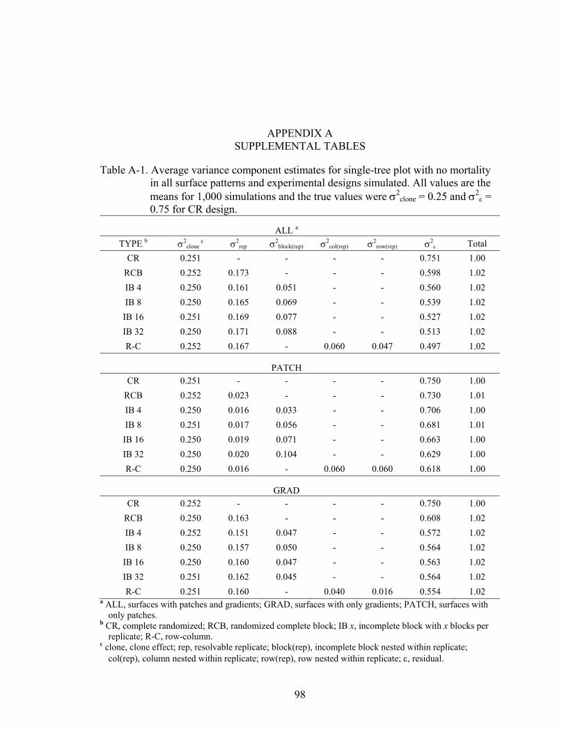
98

APPENDIX A SUPPLEMENTAL TABLES

Table A-1. Average variance component estimates for single-tree plot with no mortality in all surface patterns and experimental designs simulated. All values are the means for 1,000 simulations and the true values were σ2


0.75 for CR design.

ALL a

TYPE b σ2clone

c σ2rep σ2

block(rep) σ2col(rep) σ2

row(rep) σ2ε Total

CR 0.251 - - - - 0.751 1.00 RCB 0.252 0.173 - - - 0.598 1.02 IB 4 0.250 0.161 0.051 - - 0.560 1.02 IB 8 0.250 0.165 0.069 - - 0.539 1.02 IB 16 0.251 0.169 0.077 - - 0.527 1.02 IB 32 0.250 0.171 0.088 - - 0.513 1.02 R-C 0.252 0.167 - 0.060 0.047 0.497 1.02

PATCH


GRAD


a ALL, surfaces with patches and gradients; GRAD, surfaces with only gradients; PATCH, surfaces with only patches.

b CR, complete randomized; RCB, randomized complete block; IB x, incomplete block with x blocks per replicate; R-C, row-column.

c clone, clone effect; rep, resolvable replicate; block(rep), incomplete block nested within replicate; col(rep), column nested within replicate; row(rep), row nested within replicate; ε, residual.

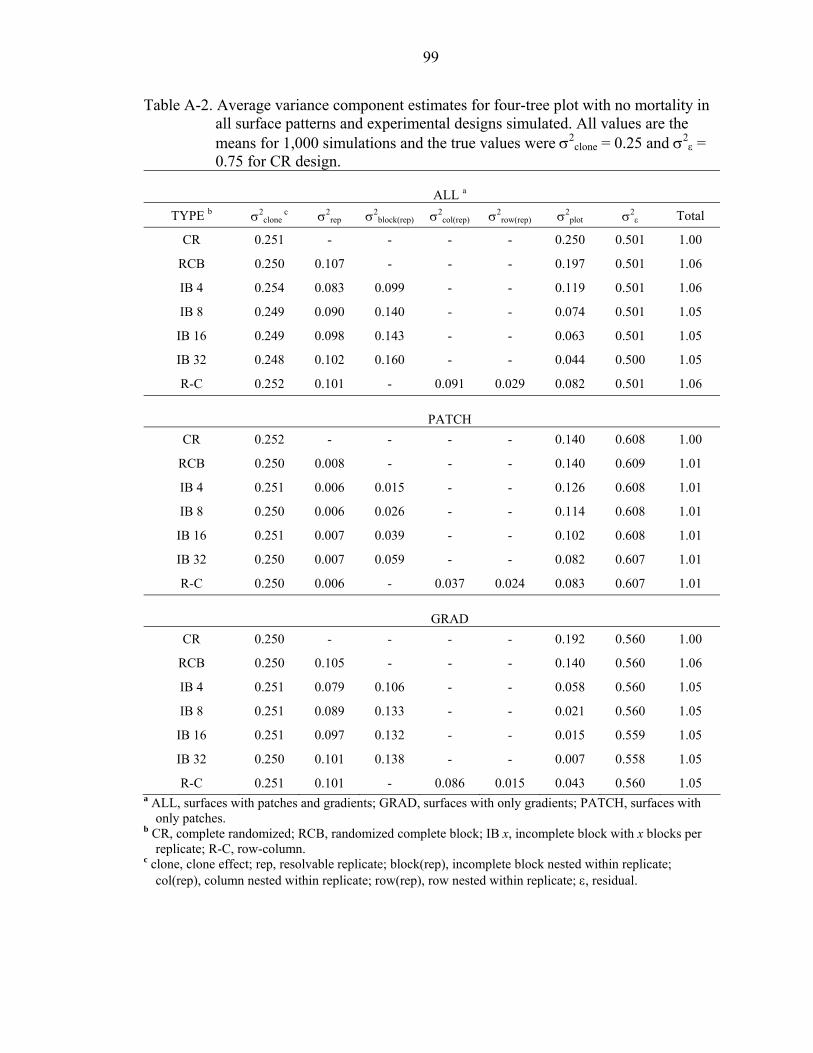
99

Table A-2. Average variance component estimates for four-tree plot with no mortality in all surface patterns and experimental designs simulated. All values are the means for 1,000 simulations and the true values were σ2


0.75 for CR design.

ALL a

TYPE b σ2clone

c σ2rep σ2


row(rep) σ2plot σ2

ε Total

CR 0.251 - - - - 0.250 0.501 1.00

RCB 0.250 0.107 - - - 0.197 0.501 1.06

IB 4 0.254 0.083 0.099 - - 0.119 0.501 1.06

IB 8 0.249 0.090 0.140 - - 0.074 0.501 1.05

IB 16 0.249 0.098 0.143 - - 0.063 0.501 1.05

IB 32 0.248 0.102 0.160 - - 0.044 0.500 1.05

R-C 0.252 0.101 - 0.091 0.029 0.082 0.501 1.06

PATCH

CR 0.252 - - - - 0.140 0.608 1.00

RCB 0.250 0.008 - - - 0.140 0.609 1.01

IB 4 0.251 0.006 0.015 - - 0.126 0.608 1.01

IB 8 0.250 0.006 0.026 - - 0.114 0.608 1.01

IB 16 0.251 0.007 0.039 - - 0.102 0.608 1.01

IB 32 0.250 0.007 0.059 - - 0.082 0.607 1.01

R-C 0.250 0.006 - 0.037 0.024 0.083 0.607 1.01

GRAD

CR 0.250 - - - - 0.192 0.560 1.00

RCB 0.250 0.105 - - - 0.140 0.560 1.06

IB 4 0.251 0.079 0.106 - - 0.058 0.560 1.05

IB 8 0.251 0.089 0.133 - - 0.021 0.560 1.05

IB 16 0.251 0.097 0.132 - - 0.015 0.559 1.05

IB 32 0.250 0.101 0.138 - - 0.007 0.558 1.05

R-C 0.251 0.101 - 0.086 0.015 0.043 0.560 1.05 a ALL, surfaces with patches and gradients; GRAD, surfaces with only gradients; PATCH, surfaces with


replicate; R-C, row-column. c clone, clone effect; rep, resolvable replicate; block(rep), incomplete block nested within replicate;


100

Table A-3. Average variance component estimates for single-tree plot with 25% mortality in all surface patterns and experimental designs simulated. All values are the means for 1,000 simulations and the true values were σ2


0.75 for CR design.

ALL a

TYPE b σ2clone

c σ2rep σ2


row(rep) σ2ε Total

CR 0.252 - - - - 0.751 1.00

RCB 0.253 0.173 - - - 0.598 1.02

IB 4 0.251 0.160 0.052 - - 0.559 1.02

IB 8 0.249 0.165 0.070 - - 0.538 1.02

IB 16 0.251 0.168 0.077 - - 0.526 1.02

IB 32 0.250 0.171 0.089 - - 0.512 1.02

R-C 0.252 0.167 - 0.061 0.048 0.495 1.02

PATCH

CR 0.251 - - - - 0.749 1.00

RCB 0.252 0.023 - - - 0.730 1.01

IB 4 0.251 0.017 0.033 - - 0.704 1.00

IB 8 0.251 0.017 0.057 - - 0.680 1.00

IB 16 0.249 0.019 0.073 - - 0.662 1.00

IB 32 0.250 0.021 0.105 - - 0.628 1.00

R-C 0.250 0.017 - 0.062 0.061 0.615 1.00

GRAD

CR 0.252 - - - - 0.750 1.00

RCB 0.250 0.163 - - - 0.607 1.02

IB 4 0.252 0.151 0.047 - - 0.573 1.02

IB 8 0.250 0.157 0.050 - - 0.564 1.02

IB 16 0.250 0.160 0.046 - - 0.563 1.02

IB 32 0.252 0.162 0.045 - - 0.563 1.02

R-C 0.250 0.160 - 0.040 0.016 0.553 1.02 a ALL, surfaces with patches and gradients; GRAD, surfaces with only gradients; PATCH, surfaces with




101

Table A-4. Average variance component estimates for four-tree plot with 25% mortality in all surface patterns and experimental designs simulated. All values are the means for 1,000 simulations and the true values were σ2


0.75 for CR design.

ALL a

TYPE b σ2clone

c σ2rep σ2


row(rep) σ2plot σ2

ε Total

CR 0.251 - - - - 0.250 0.501 1.00

RCB 0.250 0.107 - - - 0.197 0.501 1.05

IB 4 0.254 0.082 0.099 - - 0.119 0.502 1.06

IB 8 0.249 0.090 0.141 - - 0.075 0.501 1.05

IB 16 0.249 0.099 0.143 - - 0.063 0.501 1.05

IB 32 0.248 0.102 0.160 - - 0.044 0.499 1.05

R-C 0.252 0.101 - 0.092 0.030 0.081 0.501 1.06

PATCH

CR 0.252 - - - - 0.142 0.606 1.00

RCB 0.248 0.008 - - - 0.142 0.606 1.00

IB 4 0.252 0.006 0.015 - - 0.127 0.607 1.01

IB 8 0.251 0.006 0.027 - - 0.114 0.608 1.01

IB 16 0.250 0.007 0.039 - - 0.101 0.608 1.01

IB 32 0.250 0.007 0.060 - - 0.082 0.606 1.01

R-C 0.250 0.006 - 0.038 0.025 0.083 0.606 1.01

GRAD

CR 0.249 - - - - 0.192 0.560 1.00

RCB 0.251 0.105 - - - 0.139 0.559 1.05

IB 4 0.251 0.079 0.107 - - 0.057 0.561 1.05

IB 8 0.250 0.089 0.134 - - 0.022 0.558 1.05

IB 16 0.250 0.097 0.132 - - 0.017 0.559 1.05

IB 32 0.248 0.101 0.137 - - 0.010 0.557 1.05

R-C 0.249 0.100 - 0.086 0.015 0.043 0.560 1.05 a ALL, surfaces with patches and gradients; GRAD, surfaces with only gradients; PATCH, surfaces with




102

Table A-5. Average estimated correlations between true and predicted clonal (CORR) with standard deviations for 0 and 25% mortality obtained from 1,000 simulations for single-tree plots (STP) and four-tree plot row plots (4-tree) in all surface patterns and experimental designs.

0% Mortality

STP 4-tree


CR 0.853 (0.018)

0.852 (0.017)

0.853 (0.017)

0.759 (0.045)

0.796 (0.049)

0.777 (0.032)

RCB 0.877 (0.018)

0.856 (0.017)

0.876 (0.016)

0.783 (0.042)

0.799 (0.047)

0.803 (0.029)

IB 4 0.882 (0.019)

0.860 (0.018)

0.881 (0.016)

0.816 (0.032)

0.803 (0.044)

0.844 (0.019)

IB 8 0.887 (0.019)

0.862 (0.019)

0.882 (0.017)

0.841 (0.028)

0.806 (0.041)

0.865 (0.016)

IB 16 0.887 (0.021)

0.862 (0.022)

0.879 (0.017)

0.843 (0.026)

0.810 (0.039)

0.867 (0.016)

IB 32 0.887 (0.021)

0.865 (0.021)

0.879 (0.017)

0.849 (0.027)

0.816 (0.040)

0.863 (0.017)

R-C 0.888 (0.022)

0.870 (0.024)

0.879 (0.018)

0.821 (0.032)

0.817 (0.039)

0.836 (0.023)

25% Mortality

STP 4-tree


CR 0.811 (0.023)

0.809 (0.021)

0.810 (0.021)

0.724 (0.043)

0.756 (0.046)

0.739 (0.035)

RCB 0.839 (0.023)

0.814 (0.022)

0.838 (0.021)

0.747 (0.040)

0.759 (0.044)

0.764 (0.031)

IB 4 0.846 (0.025)

0.819 (0.023)

0.843 (0.022)

0.780 (0.031)

0.763 (0.041)

0.803 (0.024)

IB 8 0.850 (0.025)

0.821 (0.024)

0.845 (0.022)

0.803 (0.029)

0.765 (0.039)

0.824 (0.021)

IB 16 0.850 (0.026)

0.821 (0.026)

0.842 (0.021)

0.804 (0.027)

0.768 (0.038)

0.823 (0.022)

IB 32 0.849 (0.027)

0.824 (0.026)

0.841 (0.022)

0.807 (0.028)

0.774 (0.039)

0.819 (0.022)

R-C 0.852 (0.028)

0.829 (0.029)

0.841 (0.022)

0.781 (0.034)

0.776 (0.038)

0.794 (0.027)



103

Table A-6. Average individual broad-sense heritability calculated for single-tree plot (STP) and four-tree plot (4-tree) with their standard deviations in all surface patterns, experimental designs and mortality cases. All values are the means for 1,000 simulations and the base heritability value was 0.25 for CR design.

0% Mortality

STP 4-tree


CR 0.250 (0.026)

0.251 (0.024)

0.252 (0.025)

0.251 (0.036)

0.252 (0.032)

0.249 (0.032)

RCB 0.296 (0.033)

0.256 (0.026)

0.291 (0.030)

0.263 (0.037)

0.250 (0.031)

0.264 (0.033)

IB 4 0.309 (0.040)

0.262 (0.030)

0.305 (0.033)

0.290 (0.039)

0.255 (0.032)

0.289 (0.034)

IB 8 0.317 (0.045)

0.269 (0.034)

0.307 (0.034)

0.302 (0.040)

0.257 (0.035)

0.302 (0.034)

IB 16 0.323 (0.049)

0.273 (0.038)

0.308 (0.035)

0.306 (0.042)

0.261 (0.036)

0.304 (0.034)

IB 32 0.328 (0.055)

0.284 (0.044)

0.308 (0.035)

0.313 (0.047)

0.266 (0.039)

0.307 (0.036)

R-C 0.336 (0.060)

0.287 (0.052)

0.312 (0.035)

0.301 (0.048)

0.266 (0.041)

0.294 (0.035)

25% Mortality

STP 4-tree


CR 0.251 (0.029)

0.251 (0.027)

0.251 (0.029)

0.251 (0.041)

0.252 (0.037)

0.249 (0.038)

RCB 0.297 (0.035)

0.257 (0.030)

0.292 (0.033)

0.264 (0.042)

0.249 (0.035)

0.265 (0.038)

IB 4 0.310 (0.041)

0.263 (0.033)

0.305 (0.036)

0.290 (0.044)

0.255 (0.037)

0.289 (0.039)

IB 8 0.317 (0.047)

0.269 (0.037)

0.307 (0.037)

0.301 (0.044)

0.258 (0.038)

0.301 (0.038)

IB 16 0.323 (0.052)

0.274 (0.041)

0.308 (0.037)

0.306 (0.046)

0.261 (0.041)

0.303 (0.037)

IB 32 0.328 (0.057)

0.285 (0.047)

0.309 (0.038)

0.313 (0.051)

0.266 (0.043)

0.304 (0.040)

R-C 0.338 (0.062)

0.289 (0.055)

0.311 (0.038)

0.302 (0.051)

0.266 (0.046)

0.292 (0.038)



104

Table A-7. Coefficient of variation (100 std /⎯x) for broad-sense individual heritability obtained from 1,000 simulations with 8 ramets per clone for single-tree plot in all surface patterns and experimental designs.

ALL a

Analysis b CR c RCB IB 4 IB 8 IB 16 IB 32 R-C Average

No-LAT 10.4 % 11.2 % 12.8 % 14.2 % 15.0 % 16.5 % 17.5 % 13.9 %

Partial-LAT 10.3 % 10.9 % 12.9 % 13.7 % 15.0 % 16.2 % 17.2 % 13.7 %

Full-LAT 10.3 % 10.9 % 12.8 % 13.7 % 15.0 % 16.2 % 17.2 % 13.7 %

PATCH

Analysis CR RCB IB 4 IB 8 IB 16 IB 32 R-C Average

No-LAT 9.5 % 10.2 % 11.5 % 12.6 % 13.9 % 15.3 % 17.9 % 13.0 %

Partial-LAT 10.0 % 10.4 % 11.3 % 12.5 % 13.9 % 14.9 % 18.0 % 13.0 %

Full-LAT 10.0 % 10.4 % 11.3 % 12.5 % 13.9 % 14.9 % 17.9 % 13.0 %

GRAD

Analysis CR RCB IB 4 IB 8 IB 16 IB 32 R-C Average

No-LAT 9.9 % 10.3 % 10.9 % 11.1 % 11.2 % 11.2 % 11.3 % 10.8 %

Partial-LAT 9.6 % 10.5 % 11.0 % 11.2 % 11.3 % 11.7 % 10.9 % 10.9 %

Full-LAT 9.6 % 10.5 % 11.0 % 11.2 % 11.3 % 11.6 % 10.9 % 10.9 % a ALL, surfaces with patches and gradients; GRAD, surfaces with only gradients; PATCH, surfaces with

only patches. b No-LAT, design and analysis no Latinized; Partial-LAT, design Latinized and analysis no Latinized; Full-

LAT, design and analysis Latinized. c CR, complete randomized; RCB, randomized complete block; IB x, incomplete block with x blocks per

replicate; R-C, row-column.

105

Table A-8. Average correlations between true and predicted treatment effects (CORR) with standard deviations in parenthesis in the ALL surface patterns for 2 and 8 ramets per clone for selected experimental designs analyses and polynomial models fitted for the following error structures: independent errors (ID); autoregressive without nugget (AR1⊗AR1); and autoregressive with nugget (AR1⊗AR1+η).

ID

AR1⊗AR1

AR1⊗AR1+η

ramets / clone ramets / clone ramets / clone

Model a 2 8 2 8 2 8

CR 0.674 (0.042)

0.853 (0.018)

0.692 (0.052)

0.886 (0.024)

0.707 (0.061)

0.909 (0.023)

RCB 0.674 (0.042)

0.877 (0.017)

0.696 (0.052)

0.891 (0.024)

0.706 (0.060)

0.909 (0.024)

R-C 0.695 (0.050)

0.889 (0.022)

0.700 (0.053)

0.893 (0.024)

0.707 (0.059)

0.898 (0.025)

Full-Poly 0.692 (0.045)

0.886 (0.019)

0.702 (0.052)

0.894 (0.024)

0.709 (0.055)

0.899 (0.025)

a CR, complete randomized; RCB, randomized complete block; R-C, row-column; Full-Poly, full polynomial regression.

Table A-9. Original and post-hoc blocking average individual broad-sense heritabilities with standard deviations in parenthesis for all surface patterns obtained from fitting the models in Table 5-1 from simulated datasets with a randomized complete block design with 8 ramets per clone per site.

Original

Post-hoc


IB 4 0.309 (0.040)

0.262 (0.030)

0.305 (0.033)

0.310 (0.040)

0.263 (0.030)

0.303 (0.033)

IB 8 0.317 (0.045)

0.269 (0.034)

0.307 (0.034)

0.319 (0.045)

0.270 (0.034)

0.307 (0.034)

IB 16 0.323 (0.049)

0.273 (0.038)

0.308 (0.035)

0.323 (0.049)

0.275 (0.039)

0.307 (0.035)

IB 32 0.328 (0.055)

0.284 (0.044)

0.308 (0.035)

0.329 (0.054)

0.286 (0.043)

0.307 (0.036)

R-C 0.336 (0.060)

0.287 (0.052)

0.312 (0.035)

0.336 (0.059)

0.290 (0.053)

0.311 (0.035)

a IB x, incomplete block with x blocks per replicate; R-C, row-column. b ALL, surfaces with patches and gradients; GRAD, surfaces with only gradients; PATCH, surfaces with

only patches.

106

APPENDIX B EXTENSIONS IN CONFIDENCE INTERVALS FOR

HERITABILITY ESTIMATES

A similar study to the one performed in Chapter 4 with STP to obtain 95%

confidence intervals was performed with 4-tree row plots using the same procedures

specified before to compare empirical percentile with Dickerson’s approximation. In

addition, for both plot types approximated 95% confidence intervals where obtained for

analyses from datasets with 25% mortality.

The results indicated a surprising agreement between the empirical percentiles and

Dickerson’s approximations for 4-tree plots, particularly for GRAD surface patterns

(Figure B-1). Large differences were detected with IB 32 and R-C for surfaces with

patches (ALL and PATCH); nevertheless, these differences are irrelevant in practice.

In relation to the effects of 25% mortality, as expected, an increase in the ranges of

both 95% confidence interval approximation methods was found. This was due to an

increase in the variability of the individual heritability estimates (see Table A-6).

However, differences detected between empirical and Dickerson’s approximations for

each plot type were consistent for both levels of missing information.

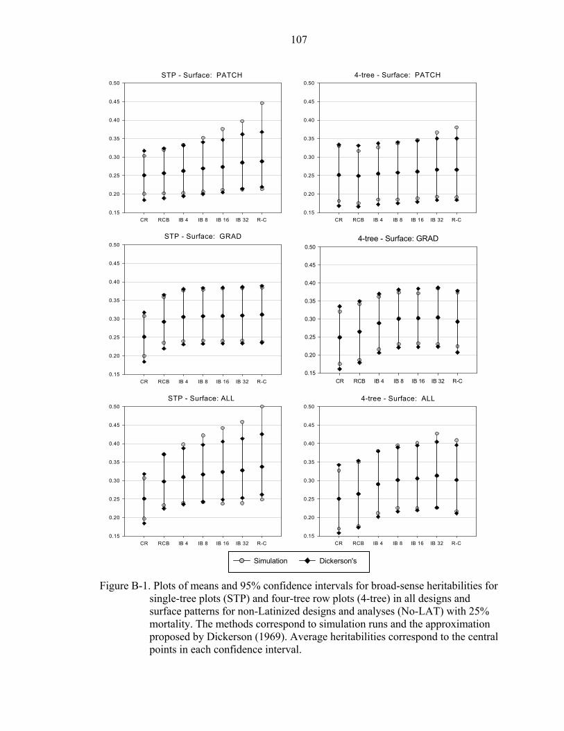
107

Simulation Dickerson's

Figure B-1. Plots of means and 95% confidence intervals for broad-sense heritabilities for

single-tree plots (STP) and four-tree row plots (4-tree) in all designs and surface patterns for non-Latinized designs and analyses (No-LAT) with 25% mortality. The methods correspond to simulation runs and the approximation proposed by Dickerson (1969). Average heritabilities correspond to the central points in each confidence interval.

4-tree - Surface: PATCH


0.20

0.25

0.30

0.35

0.40

0.45

0.50STP - Surface: PATCH


0.20

0.25

0.30

0.35

0.40

0.45

0.50

4-tree - Surface: GRAD


0.20

0.25

0.30

0.35

0.40

0.45

0.50

STP - Surface: ALL


0.20

0.25

0.30

0.35

0.40

0.45

0.50

STP - Surface: GRAD


0.20

0.25

0.30

0.35

0.40

0.45

0.50

4-tree - Surface: ALL


0.20

0.25

0.30

0.35

0.40

0.45

0.50

108

APPENDIX C MATLAB SOURCE CODE

Annotated Matlab Code to Generate Error Surfaces

function ZST=ar2(n,m,RHOX,RHOY,a,b,s20,e1,e2); % Program that generates the error surfaces % Modified for Exponential = AR(1)xAR(1) (Anisotropic) % Incorporates Polynomial Function for Mean Vector. % Salvador A. Gezan / Dec-2005 % n: number of rows % m: number of columns % RHOX: spatial correlation in the x-direction % RHOY: spatial correlation in the y-direction % a, b: parameters polynomial trend regression % s20: nugget effect error % e1, e2: independent vectors of errors rand('state',sum(100*clock)) s2=1; N=n*m; V=eye(N,N); % Calculation of base V(N*N) MATRIX with AR(1)*AR(1) covariance model Y=zeros(N,1);X=zeros(N,1); for K=1:N Y1=fix((K-1)/m)+1; % I X1=K-(Y1-1)*m; % J Y(K)=Y1;X(K)=X1; % Recording Position for L=K+1:N Y2=fix((L-1)/m)+1; X2=L-(Y2-1)*m; V(K,L)=s2*(RHOXâbs(X2-X1))*(RHOYâbs(Y2-Y1)); % Core AR(1)xAR1(1) V(L,K)=V(K,L); end end % Generation of correlated errors (using Cholesky decomposition) L=chol(V); PAT=L'*e1; PAT=(PAT-mean(PAT))/std(PAT); % Standarized Patches % Incorporation trend and production Surface if a==0 & b==0 Z=PAT; else XC=X-mean(X);YC=Y-mean(Y); mu=a*(XC+YC)+b*((XC.^2).*YC+XC.*(YC.^2)); mu=(mu-mean(mu))/std(mu); % Standarized means (trends) Z=(mu+PAT)./sqrt(2); % Standarized surface end;

109

% Incorporating Nugget (white noise) ZST=Z*sqrt(1-s20)+e2*sqrt(s20); % Drawing simulated Surface for I=1:n*m; SUR(Y(I),X(I))=ZST(I); end surf(SUR); view(45,30);axis equal; xlabel('X');ylabel('Y');

Annotated Matlab Code to Generate Clonal Trials

function CHARS=SIMULA(FORM,NSETS); % Program that generates the clonal trial datasets ready for analysis % Implemented for single site analyses % Salvador A. Gezan / Dec-2005 % Calls files: % SURFALL.TXT Contains 500 surfaces as vectors % Structure: X Y S1 S2 ... S499 S500 % PARAMALL.TXT Contains parameters from surfaces simulated for ALL pattern % PARAMFLAT.TXT Contains parameters from surfaces simulated for ALL pattern % PARAMGRAD.TXT Contains parameters from surfaces simulated for ALL pattern % Structure: SURF RHOX RHOY a b S20 % VALGEN.MAT 500*256 matrix with random clonal genetic values ~N(0,1) % GXENV.MAT 500*256 matrix with random genotype x environment % interactions ~N(0,1) % n: number of rows % m: number of columns % NSETS: number of simulations to be generated % FORM: Plot Type: Single Tree Plot (FORM=1) % 4-tree row Plot (FORM=2) % DSGPTYPE: experimental design type % 1:CR, 2:RCB, 3:IB4, 4:IB8, 5:IB16, 6:IB32, 7:R-C % LATIN: Latinization type % 0:No-Latinized, 1:Latinized % RNDSTP(TYPE,LAT,SET): Function that calls pre-generated CycDesigN for STP % RNDROW(TYPE,SET): Function that calls pre-generated CycDesigN for 4-tree rand('state',sum(100*clock)) % Reading Files SURFS=load('SURFALL.TXT'); % Simulated surfaces SURFS=sortrows(SURFS,[1 2]); PARAM=load('PARAMALL.TXT'); % Parameters of simulated surfaces load VALGEN.MAT % Random vectors of clonal values load GXENV.MAT % Random vectors of gxe interactions % Inicialization n=64; m=32; N=n*m; % Total number of observation CHARS=[]; % Output Matrix SELVG=zeros(500,1); % Selection Vector for Clonal Values SELGXE=zeros(500,1); % Selection Vector for GXE Interaction IDVG=ceil(rand(1)*500); % Random starting vector for clonal values IDGXE=ceil(rand(1)*500);% Random starting vector for gxe interactions

110

RESP=[]; for SET=1:NSETS % Reads set of Clonal Values IDVG=IDVG+1; if IDVG>500;IDVG=IDVG-500;end BV=VALGEN(:,IDVG); % Reads set of GXE interactions IDGXE=IDGXE+1; if IDGXE>500;IDGXE=IDGXE-500;end GXE=GXENV(:,IDGXE); % Reads SURFACE consecutively ZSUR=SURFS(:,SET+2); X=SURFS(:,1); % x positions in test Y=SURFS(:,2); % y positions in test % Generation of Effects for linear model mu=10; %Population Mean (arbitrary) BV=sqrt(0.20)*BV; % 0.20 s2clone (multiple sites) GXE=sqrt(0.05)*GXE; % 0.05 s2gxe ZSUR=sqrt(0.75)*ZSUR; % 0.75 s2s+s2ms (total error) DSGPTYPE=[1 2 3 4 5 6 7]; for TYPE=1:7 for FORM=1:2 for LATIN=0:1 %Latinization LAT='A'; if LATIN==1;LAT='L';end if FORM==2 & LAT=='L';break;end % Gets pre-generated design (CycDesigN) % Structure NDES:REP BLK PLT TREE LAT CLONE X Y (DSGTYPE 1-6) % Structure NDES:REP ROW COL TREE LROW LCOL CLONE X Y (DSGTYPE 7) if FORM==1 %STP NDES=RNDSTP(TYPE,LAT,SET); elseif FORM==2 %4-tree NDES=RNDROW(TYPE,SET); end % Calculation of Response Values (Yijkl) RESP0=[zeros(size(NDES)) zeros(N,1)]; for I=1:N %Assigns clonal value (VG) and GXE to each CLONE if TYPE==7 VG=BV(NDES(I,7)); GE=GXE(NDES(I,7)); else VG=BV(NDES(I,6)); GE=GXE(NDES(I,6)); end YA=mu+VG+GE+ZSUR(I); % Final response vector % Structure RESP0: REP BLK PLOT TREE LAT (LCOL) CLONE X Y YA % Structure RESP0: REP ROW COL TREE LAT (LCOL) CLONE X Y YA RESP0(I,:)=[NDES(I,:) YA]; % Adds columns with levels of design end

111

% Saving Final simulated trial file (RESP0) if SET<10 RUN=['00' num2str(SET)]; elseif SET<100 & SET>=10 RUN=['0' num2str(SET)]; else RUN=num2str(SET); end FNAME=[LAT RUN 'T' num2str(TYPE) 'F' num2str(FORM) '.TXT']; if TYPE==7

FFORMAT='%3.0f %3.0f %4.0f %2.0f %3.0f %3.0f … %3.0f %3.0f %3.0f %10.6f \n';

else FFORMAT='%3.0f %3.0f %4.0f %2.0f %3.0f %3.0f … %3.0f %3.0f %10.6f \n';

end fid = fopen(FNAME,'wt'); fprintf(fid,FFORMAT,RESP0'); fclose(fid); end end end % Stores parameters of simulated surface and random vectors used % Structure: SET IDVG IDGXE RHOX RHOY a b S20 CHARS=[CHARS;SET IDVG IDGXE PARAM(SET,2:6)]; end % Saving file of Parameters (CHARS) FNAME='SIMALL.TXT'; FFORMAT='%4.0f %4.0f %4.0f %6.4f %6.4f %6.4f %8.6f %6.4f \n'; fid = fopen(FNAME,'wt'); fprintf(fid,FFORMAT,CHARS'); fclose(fid);

112

LIST OF REFERENCES

Atkinson, A.C. 1969. The use of residuals as a concomitant variable. Biometrika 56(1): 33-41.

Ball, S.T., Mulla, D.J., and Konzak, C.F. 1993. Spatial heterogeneity affects variety trial interpretation. Crop Sci. 33: 931-935.

Bartlett, M.S. 1978. Nearest neighbour models in the analysis of field experiments. J. R. Statist. Soc. B 40(2): 147-174.

Binns, M.R. 1987. Practical use of neighbor methods and alternatives in the analysis of field trials. Can. J. Plant. Sci. 67: 477-489.

Bonga, J.M., and Park, Y.S. 2003. Clonal propagation, forest trees. In: Thomas, B., Murphy, D, and Murray, B. (Eds). Encyclopedia of applied plant sciences. Elsevier Science Ltd. Oxford, U.K. pp. 1395-1402.

Box, G.E.P, and Hay, W.A. 1953. A statistical design for the efficient removal of trends occurring in a comparative experiment with an application in biological assay. Biometrics 9: 304-319.

Brownie, C., Bowman, D.T., and Burton, J.W. 1993. Estimating spatial variation in analysis of data from yield trials: a comparison of methods. Agron. J. 85: 1244-1253.

Brownie. C., and Gumpertz, M.L. 1997. Validity of spatial analyses for large field trials. J. Agric. Biol. Environ. Stat. 2(1): 1-23.

Carson, M.J. 1986. Advantages of clonal forestry for Pinus radiata – real or imagined? New Zeal. J. For. Sci. 16: 403-415.

Cleveland, W.S. 1979. Robust locally weighted regression and smoothing scatterplots. J. Amer. Statist. Assoc. 74: 829-836.

Cochran, W.G. 1957. Analysis of covariance: its nature and uses. Biometrics 13: 261-281.

Cochran, W.G., and Cox, G.M. 1957. Experimental designs. 2nd ed. John Wiley & Sons, Inc. New York. 611pp.

113

Costa e Silva, J., Dutkowski, G.W., and Gilmour, A.R. 2001. Analysis of early tree height in forest genetic trials is enhanced by including a spatially correlated residual. Can. J. For. Res. 31: 1887-1893.

Cressie, N.A.C. 1993. Statistics for spatial data – revised edition. John Wiley & Sons, Inc. New York. 900pp.

Cullis, B.R., and Gleeson, A.C. 1991. Spatial analysis of field experiments – an extension to two dimensions. Biometrics 47: 1449-1460.

Dickerson, G.E. 1969. Techniques for research in quantitative animal genetics. In: Techniques and procedures in animal science research. Amer. Soc. Anim. Sci. Albany, New York. pp. 36-79.

Dieters, M.J. 1994. Inheritance of volume and rust resistance in slash pine. Ph.D. Dissertation, University of Florida, Gainesville, Florida. 104pp.

Durbán, M., Hackett, C., and Currie, I. 1999. Blocks, trend and interference in field trials. In: Friedl, H., Berghold, A., and Kauermann, G. (Eds.). Proceedings of 14th International Workshop on Statistical Modelling. Graz, Austria. July 19-23, 1999. pp. 492-495.

Dutkowski, G.W., Costa e Silva, J., Gilmour, A.R., and Lopez, G.A. 2002. Spatial analysis methods for forest genetic trials. Can. J. For. Res. 32: 2201-2214.

Elridge, K., Davidson, J., Harwood, C., and van Wyk, G. 1993. Eucalypt domestication and breeding. Clarendon Press. Oxford, U.K. 288pp.

Ericsson, T. 1997. Enhanced heritabilities and best linear unbiased predictors through appropriate blocking of progeny trials. Can. J. Forest. Res. 27: 2097-2101.

Falconer, D.S., and Mackay, T.F.C. 1996. Introduction to quantitative genetics. 4th ed. Prentice Hall. Harlow, U.K. 464pp.

Federer, W.T. 1988. Recovery of interblock, intergradient, and intervariety information in incomplete block and lattice rectangle design experiments. Biometrics 54: 471-481.

Fu, Y.B., Clarke, G.P.Y., Namkoong, G., and Yanchuk, A.D. 1998. Incomplete block designs for genetic testing: statistical efficiencies of estimating family means. Can. J. For. Res. 28: 977-986.

Fu, Y.B., Yanchuk, A.D., and Namkoong, G. 1999a. Incomplete block designs for genetic testing: some practical considerations. Can. J. Forest. Res. 29: 1871-1878.

Fu, Y.B., Yanchuk, A.D., Namkoong, G., and Clarke, G.P.Y. 1999b. Incomplete block designs for genetic testing: statistical efficiencies with missing observations. For. Sci. 45(3): 374-380.

114

Gilmour, A.R., Cullis, B.R., and Verbyla, A.P. 1997. Accounting for natural and extraneous variation in the analysis of field experiments. J. Agric. Biol. Environ. Stat. 2(3): 269-293.

Gilmour, A.R., Gogel, B.J., Cullis, B.R., Welham, S.J., and Thompson, R. 2002. ASReml User guide release 1.0. VSN International Ltd. Hemel Hempstead, HP1 1ES, UK. 267pp.

Grondona, M.O., and Cressie, N. 1991. Using spatial considerations in the analysis of experiments. Technometrics 33(4): 381-392.

Grondona, M.O., Crossa, J., Fox, P.N., and Pfeiffer, W.H. 1996. Analysis of variety yield trials using two-dimensional separable ARIMA processes. Biometrics 52: 763-770.

John, J.A., and Williams, E.R. 1995. Cyclic and computer generated designs. Monographs on Statistics and Applied Probability 38. Chapman & Hall. London, U.K. 255pp.

Johnson, M.E. 1987 Multivariate statistical simulation. John Wiley & Sons, Inc. New York. 230pp.

Kempton, R.A., and Howes, C.W. 1981. The use of neighbouring plot values in the analysis of variety trials. Appl. Statist. 30(1): 59-70.

Libby, W.J. 1977. Rooted cuttings in production forests. In: Proc. 14th Southern Forest Tree Improvement Conference, Gainesville, Florida. pp. 13-27.

Libby, W.J., and Rauter, R.M. 1984. Advantages of clonal forestry. For. Chron. 60: 145–149.

Lin, C.S., Binns, M.R., Voldeng, H.D., and Guillemette, R. 1993. Performance of randomized block designs in field experiments. Agron. J. 65: 168-171.

Littell, R.C., Milliken, G.A., Stroup, W.W., and Wolfinger, R.D. 1996. SAS® system for mixed models. SAS Institute Inc. Cary, North Carolina. 633pp.

Loo-Dinkins, J., Tauer, C.G., and Lambeth, C.C. 1990. Selection system efficiencies for computer simulated progeny test field designs in loblolly pine. Theor. Appl. Genet. 79: 89-96.

Lopez, G.A., Potts, B.M., Dutkowski, G.W., Apiolaza, L.A., and Gelid, P.E. 2002. Genetic variation and inter-trait correlations in Eucalyptus globulus base population trials in Argentina. Forest Genetics 9(3): 217-231.

Lui, B.H., Knapp, S.J., and Birkes, D. 1997. Sampling distributions, biases, variances, and confidence intervals for genetic correlations. Theor. Appl. Genet. 94: 8-19.

115

Magnussen, S. 1993. Bias in genetic variance estimates due to spatial variation. Theor. Appl. Genet. 86: 349-355.

MathWorks. 2000. Using MATLAB Version 6.0. The MathWorks, Inc. Natick, Massachusetts. 874pp.

Namkoong, G. 1979. Introduction to quantitative genetics in forestry. USDA Forest Service Technical Bulletin N° 1588. Washington, District of Columbia. 342pp.

Ndlovu, P. 1992. Classical and bootstrap estimates of heritability of milk yield in Zimbabwean Holstein cows. J. Diary. Sci. 76: 2013-2024.

Patterson, H.D., and Hunter, E.A. 1983. The efficiency in incomplete block design in national list and recommended list cereal variety trials. J. Agric. Sci. 101: 427-433.

Patterson, H.D., and Thompson, R. 1971. Recovery of inter-block information when block sizes are unequal. Biometrika 58: 545-554.

Pearce, S.C. 1976. The conduct of “post-mortems” on concluded field trials. Expl. Agric. 12: 151-162.

Pearce, S.C. 1998. Field experimentation on rough land: the method of Papadakis reconsidered. J. Agric. Sci. 131:1-11.

Pearce, S.C., Clarke, G.M., Dyke, G.V., and Kempson, R.E. 1988. A manual of crop experimentation. Charles Griffin & Company Limited. London, UK. 358pp.

Qiao, C.G., Basford, K.E., DeLacy, I.H., and Cooper, M. 2000. Evaluation of experimental designs and spatial analysis in wheat breeding trials. Theor. Appl. Genet. 100: 9-16.

Ritchie, G.A. 1992. The commercial use of conifer rooted cuttings in forestry: a world review. New For. 5: 247-275.

Russell, J.H., and Libby, W.J. 1986. Clonal testing efficiency: the trade-offs between clones tested and ramets per clone. Can. J. For. Res. 16: 925-930.

Russel, J.H., and Loo-Dinkins, J.A. 1993. Distribution of testing effort in cloned genetic tests. Silvae Genetica 42: 98-104.

Sarker, A., Singh, M., and Erskine, W. 2001. Efficiency of spatial methods in yield trials in lentil (Lens culinaris ssp. culinaris). J. Agric. Sci. 137: 427-438.

Scharf, P.C., and Alley, M.M. 1993. Accounting for spatial yield variability in field experiments increases statistical power. Agron. J. 85: 1254-1256.

Searle, S.R., Casella, G., and McCulloch, C.E. 1992. Variance components. John Wiley & Sons, Inc. New York. 501pp.

116

Shaw, D.V., and Hood, J.V. 1985. Maximizing gain per effort by using clonal replicates in genetic tests. Theor. Appl. Genet. 71: 392-399.

Stroup, W.W., Baenziger, P.S., and Mulitze, D.K. 1994. Removing spatial variation from wheat yield trials: a comparison of methods. Crop Sci. 86: 62-66.

Townley-Smith, T.F., and Hurd, E.A. 1973. Use of moving means in wheat yield trials. Can. J. Plant. Sci. 53: 447-450.

Verbyla, A.P., Cullis, B.R., Kenward, M.G., and Welham, S.J. 1999. The analysis of designed experiments and longitudinal data by using smoothing splines. Appl. Statist. 48(3): 269-311.

Vollmann, J., Buerstmayr, H., and Ruckenbauer, P. 1996. Efficient control of spatial variation in yield trials using neighbor plot residuals. Exp. Agric. 32: 185-197.

Whitaker, D., Williams, E.R., and John, J.A. 2002. CycDesigN: a package for the computer generation of experimental designs. Version 2.0. CSIRO. Canberra, Australia. 33pp.

White, T.L. 2004. Breeding theory and genetic testing. In: Burley, J., Evans, J., and Youngquist, J.A. (Eds). Encyclopedia of forest sciences. Elsevier Science Ltd. Oxford, U.K. pp. 1551-1561.

Wilkinson, G.N., Eckert, S.R., Hancock, T.W., and Mayo, O. 1983. Nearest neighbour (NN) analysis of field experiments. J. R. Statist. Soc. B 45(2): 151-211.

Williams, E.R. 1985. A criterion for the construction of optimal neighbor designs. J. R. Statist. Soc. B 47(3): 489-497.

Williams, E.R., and Fu, Y.B. 1999. Comment - Enhanced heritabilities and best linear unbiased predictors through appropriate blocking of progeny trials. Can. J. Forest. Res. 29: 1633-1634.

Williams, E.R., and John, J.A. 1996. Row-column factorial designs for use in agricultural field trials. Appl. Statist. 45(1): 39-46.

Williams, E.R., John, J.A., and Whitaker, D. 1999. Example of block designs for plant and tree breeding trials. Aust. N. Z. J. Stat. 41(3): 277-284.

Williams, E.R., Matheson, A.C., and Harwood, C.E. 2002. Experimental design and analysis for tree improvement. Second Edition. CSIRO Publishing. Collingwood, Australia. 214pp.

Wolfinger, R.D. 1996. Heterogeneous variance-covariance structures for repeated measures. J. Agric. Biol. Environ. Stat. 1(2): 205-230.

117

Young, L.J., and Young, J.H. 1998. Statistical ecology: a population perspective. Kluwer Academic Publishers. Boston, Massachusetts. 565pp.

Zimmerman, D.L., and Harville, D.A. 1991. A random field approach to the analysis of field-plot experiments and other spatial experiments. Biometrics 47: 223-239.

Zobel, B.J., and Talbert, J.T. 1984. Applied forest tree improvement. John Wiley & Sons, Inc. New York. 505pp.

118

BIOGRAPHICAL SKETCH

Salvador Alejandro Gezan was born in October 13, 1973, in Santiago, Chile, a

polluted city flanked by the Andes. After a few moths, his family moved to Mexico, to

settle first in Acapulco and later in Mexico City, where he practically became a Mexican

boy. After 10 years he returned to his still “unknown” home country to the city of

Santiago to live during a few years of political repression and later the happy times of the

return to democracy. By 1996 he finished his Bachelor of Science in forestry from the

Universidad de Chile in Santiago. A few months later, after being involved in temporary

and dubious activities, he obtained a research position at the Universidad Austral de Chile

in the rainy but pretty city of Valdivia. His job consisted of building a growth and yield

simulator for native forests, which he enjoyed considerably. After 3 years of mud and wet

cold shoes in January of 2001, he started a Ph.D. program in the USA at the University of

Florida in the wet, hot and flat city of Gainesville. There, he was lucky to work with two

of his most favorite topics, forestry and statistics; nevertheless, at times he was distracted

by sports activities such as triathlon. Finally, after 21 years and thanks to the monetary

support of several (almost uninterested) sources he was able to end his school work.

Documents

OPTIMAL DESIGN AND ANALYSIS OF CLONAL FORESTRY