Optimal Control of the Atmospheric Reentry of a Space

HAL Id: inria-00317722https://hal.inria.fr/inria-00317722

Submitted on 3 Sep 2008

HAL is a multi-disciplinary open accessarchive for the deposit and dissemination of sci-entific research documents, whether they are pub-lished or not. The documents may come fromteaching and research institutions in France orabroad, or from public or private research centers.

L’archive ouverte pluridisciplinaire HAL, estdestinée au dépôt et à la diffusion de documentsscientifiques de niveau recherche, publiés ou non,émanant des établissements d’enseignement et derecherche français ou étrangers, des laboratoirespublics ou privés.

Optimal Control of the Atmospheric Reentry of a SpaceShuttle by an Homotopy Method

Audrey Hermant

To cite this version:Audrey Hermant. Optimal Control of the Atmospheric Reentry of a Space Shuttle by an Ho-motopy Method. Optimal Control Applications and Methods, Wiley, 2011, 32 (6), pp.627-646.10.1002/oca.961. inria-00317722

https://hal.inria.fr/inria-00317722

https://hal.archives-ouvertes.fr

appor t de r ech er ch e

ISS

N02

49-6

399

ISR

NIN

RIA

/RR

--66

27--

FR

+E

NG

Thème NUM

INSTITUT NATIONAL DE RECHERCHE EN INFORMATIQUE ET EN AUTOMATIQUE

Optimal Control of the Atmospheric Reentry of aSpace Shuttle by an Homotopy Method

Audrey Hermant

N° 6627

September 2008

Centre de recherche INRIA Saclay – Île-de-FranceParc Orsay Université

4, rue Jacques Monod, 91893 ORSAY CedexTéléphone : +33 1 72 92 59 00

Optimal Control of the Atmospheric Reentry of a

Space Shuttle by an Homotopy Method

Audrey Hermant∗

Theme NUM — Systemes numeriquesEquipes-Projets Commands

Rapport de recherche n° 6627 — September 2008 — 23 pages

Abstract: This paper deals with the optimal control problem of the atmospheric reentryof a space shuttle with a second-order state constraint on the thermal flux. We solve theproblem using the shooting algorithm combined with an homotopy method which auto-matically determines the structure of the optimal trajectory (composed of one boundaryarc and one touch point).

Key-words: Optimal control, State constraint, Shooting algorithm, Homotopy method,Atmospheric reentry.

∗ CMAP, Ecole Polytechnique, INRIA Saclay Ile-de-France, Route de Saclay, 91128 Palaiseau, France.

Commande optimale de la rentree atmospherique

d’une navette spatiale par une methode d’homotopie

Resume : Dans cet article, on s’interesse au probleme de commande optimale de la rentreeatmospherique d’une navette spatiale avec une contrainte sur l’etat du second ordre surle flux thermique. Le probleme est resolu par l’algorithme de tir combine a une methoded’homotopie qui determine automatiquement la structure de la trajectoire (composee d’unarc frontiere et d’un point de contact isole).

Mots-cles : Commande optimale, contrainte sur l’etat, algorithme de tir, methoded’homotopie, rentree atmospherique.

Optimal Control of the Atmospheric Reentry of a Space Shuttle 3

1 Introduction

The optimal control of the atmospheric reentry of a space shuttle is a challenging opti-mal control problem. It has been studied by many authors and solved using either directmethods (nonlinear programming), see [3, 7, 13], or indirect methods (multiple shooting),see [9, 15, 16]. Shooting methods, based on the resolution of a two- (or multi-) pointsboundary value problem, are choice methods when a high precision is required to computea reliable optimal trajectory. However, it is well known that due to a small domain ofconvergence, it may be difficult to initialize the unknown variables to make the shoot-ing algorithm converge. Moreover, in presence of constraints, the a priori knowlegde ofthe structure of constraints is required. To overcome these difficulties, continuations orhomotopy methods can be used (see [1]), starting the homotopy path from an easier prob-lem, e.g. the unconstrained problem (i.e. the problem without the state constraint), andintroducing the constraints progressively, see e.g. [2, 11].

In the course of homotopy, the structure of solutions may vary, as well as the dimen-sion of the unknown vector of shooting parameters. At those points where the structurechanges, classical continuation methods cannot be applied. Somehow heuristic rules (jus-tified in practice) for updating the structure of the trajectory were given e.g. in [2]. It isof interest to be able to describe those changes in the structure for general control prob-lems. Such results have been obtained in [5] for first-order state constraints and in [12]for second-order state constraints, providing a solid basis for a new homotopy algorithmwhich automatically determines the structure of the constraint and initializes the associ-ated shooting parameters. The user has only to provide an initial guess for the solution ofthe unconstrained problem.

Our aim in this work is to illustrate this algorithm on the problem of the atmosphericreentry of a space shuttle with a second-order state constraint on the thermal flux. Wefollow the model of Bonnard, Faubourg, Trelat [9]. In [9], the authors computed anapproximate solution by assuming that the control is bang-bang on interior arcs. (As itcan be seen on Figure 5(a), this approximation is justified.) This simplification allows theauthors to deduce the structure of the trajectory using a geometric analysis (see [10, 8])and to obtain the solution by a shooting method without introducing the adjoint variables.In the present paper, we are able to check that the control is continuous (see Lemma 8)and that the Legendre-Clebsch condition holds excepted at the final time. The full setof necessary conditions is solved by the shooting algorithm. To this end, the geometricanalysis in [10, 8] is used to initialize the unconstrained problem. Then we apply thehomotopy algorithm of [12] which successfully finds the structure of the optimal trajectory,composed of one boundary arc and one touch point.

The paper is organized as follows. In section 2, the optimal control framework and thehomotopy algorithm are presented. In section 3, we recall the model of [9] and discussthe validity of the assumptions of the homotopy algorithm. In section 4, we detail theinitialization of the unconstrained problem. Finally, in section 5, we present the resolutionof the constrained problem and give some comments on the numerical implementation.

RR n° 6627

4 A. Hermant

2 Homotopy algorithm

2.1 General framework

We consider general optimal control problems with a scalar control and scalar state con-straint of the following form:

(P) min

∫ tf

0

ℓ(u(t), y(t))dt (1)

subject to y(t) = f(u(t), y(t)) for a.a. t ∈ [0, tf ], (2)

g(y(t)) ≤ 0 for all t ∈ [0, tf ], (3)

ψ(y(0), y(tf )) = 0, (4)

u(t) ∈ U (5)

where the controls u(·) are measurable and bounded functions, U is a closed and convexsubset of R and ℓ : R × R

n → R, f : R × Rn → R

n, g : Rn → R, and ψ : R

2n → Rr are

smooth functions. The classical (resp. generalized) Hamiltonian H : R × Rn × R

n∗ → R

(resp. H : R × R × Rn × R

n∗ → R) of problem (P) are defined by

H(u, y, p) := ℓ(u, y) + pf(u, y), (6)

H(p0;u, y, p) := p0ℓ(u, y) + pf(u, y). (7)

The well-known optimality condition of problem (P) is as follows.

Definition 1. We say that (u, y) is a Pontryagin extremal, if there exists p0 ∈ R+, functionsp : [0, tf ] → R

n∗ and η : [0, tf ] → R of bounded variation such that η(tf ) = 0, and λ ∈ Rr∗,

(p0, p, η, λ) not all zero, such that

y = f(u, y), (8)

−dp = Hy(p0;u, y, p)dt+ gy(y)dη, (9)

u(t) ∈ argminw∈UH(p0;w, y, p), (10)

0 ≥ g(y(t)), dη ≥ 0,∫ T

0g(y(t))dη(t) = 0, (11)

0 = ψ(y(0), y(tf )), p(0) = −λψy0(y(0), y(tf )), p(tf ) = λψytf(y(0), y(tf )). (12)

Moreover, if the final time tf is free,

minw∈U

H(p0;w, y(tf ), p(tf )) = 0. (13)

Theorem 2. An optimal trajectory of (P) is a Pontryagin extremal.

The contact set of the constraint is defined by I(g(y)) := t ∈ [0, tf ] : g(y(t)) = 0. Weconsider the following assumptions:

(A1) The functions ℓ, ψ and f (resp. g) are C3 (resp. C4) with locally Lipschitz continuousthird-order (resp. fourth-order) derivatives.

(A2) The control u is continuous and (strengthened Legendre-Clebsch condition)

∃ α > 0, Huu(u(t), y(t), p(t)) ≥ α for all t ∈ [0, tf ]. (14)

(A3) The state constraint is a regular state constraint of second-order. This means that thefirst-order time derivative of the constraint defined by g(1)(u, y) := gy(y)f(u, y) does

not depend on the control variable, i.e. g(1)u is identically zero, while the second-order

time derivative defined by g(2)(u, y) := g(1)y (y)f(u, y) satisfies

∃ α, σ > 0, |g(2)u (u(t), y(t))| ≥ α for all t : distt; I(g(y)) < σ. (15)

INRIA


2.2 Description of the homotopy algorithm

In this section we present the homotopy algorithm. Throughout the section it is assumedthat U = R, i.e. the control is unconstrained. We start by some definitions.

The structure of a trajectory is the number and order of boundary arcs (time intervals(τen, τex) where g(y(t)) = 0) and touch points (isolated times τto such that g(y(τto)) = 0).The left- and right endpoints of a boundary arc (τen, τex) are called respectively entryand exit points. A touch point τ is said to be essential if [η(τ)] > 0 and reducible ifg(2)(u(τ), y(τ)) < 0.

The shooting algorithm Let us first recall the shooting algorithm for optimal controlproblems with a second-order state constraint (see [14, 6, 15]). The alternative multipli-ers used in the shooting algorithm are denoted by p2, η2 and we define the alternativeHamiltonian H : R × R

n × Rn∗ × R → R by

H(u, y, p2, η2) := H(u, y, p2) + η2g(2)(u, y)

where H is the classical Hamiltonian (6). Througout the section, it is assumed thatassumptions (A1)–(A3) hold and that

(A4) The trajectory has finitely many boundary arcs and finitely many touch points andthe state constraint is not active at initial and final times, i.e. g(y(0)) < 0 andg(y(tf)) < 0.

Moreover, we assume that the extremals are normal, i.e. p0 = 1, and hence Pontryagin’sminimum principle holds by substituting to the generalized Hamiltonian H the classicalHamiltonian H .

Remark 3. Under our assumptions, the Hamiltonian is constant along a Pontryagin ex-tremal so that (13) is equivalent to, for any t∗ ∈ [0, tf ] (in particular t∗ = 0)

H(u(t∗), y(t∗), p(t∗)) = 0.

Assume that the structure of the trajectory is known and given e.g. by the variableS := [s1, . . . , sN ] where the size N is variable, si ∈ 1, 2 for i = 1, . . . , N , and “1”stands for a touch point and “2” for a boundary arc. Then the dimension of the shootingfunction is given by dS := 2n + r + 1 + (2n + 2)

∑N

i=1 si. More precisely, a vector ofshooting parameters θ ∈ R

dS and the shooting function FS : RdS → R

dS associated withthe structure S are as follows:

θ :=

y0

p0

λtfa1

...aN

, FS(θ) :=

p0 + λψy0(y0, y(tf ))

p2(tf ) − λψytf(y0, y(tf ))

ψ(y0, y(tf ))H(u(0), y(0), p(0))

b1...bN

where (y0, p0) is the initial value of state and costate, λ is the multiplier associated withthe constraint (4), tf is the (free) final time, and, for i = 1, . . . , N , ai, bi ∈ R

(2n+2)si areas follows. If si = 1 (touch point τ i

to):

ai =

νito

τ ito

yito

pito

, bi =

g(y(τ ito))

g(1)(y(τ ito))

yito − y(τ i

to)

pito − p(τ i−

to ) + νitogy(y(τ i

to))

RR n° 6627

6 A. Hermant

where νito is the jump parameter of the costate and (yi

to, pito) the state-costate value at

touch point τ ito. If si = 2 (boundary arc (τ i

en, τ iex)):

ai =

ν1,ien

ν2,ien

τ ien

yien

pien

τ iex

yiex

piex

, bi =

g(y(τ ien))

g(1)(y(τ ien))

g(2)(u(τ i−en ), y(τ i

en)),

yien − y(τ i

en)

pien − p(τ i−

en ) + ν1,ien gy(y(τ i

en)) + ν2,ien g

(1)y (y(τ i

en))

g(2)(u(τ i+ex ), y(τ i

ex))

yiex − y(τ i

ex)

piex − p(τ i

ex)

.

where ν1,ien , ν2,i

en are the jump parameters of the costate at entry times, and (yien, p

ien) and

(yiex, p

iex) are the state-costate values at respectively entry and exit points. The trajectory

and multipliers (y, u, p2, η2) are the solution of, on the interior of each arc (τ, τ ′) (which isa boundary arc if (τ, τ ′) = (τ i

en, τiex) and an interior arc if τ is one of 0, τ i

to, or τ iex and τ ′

is one of τ i+1to , τ i+1

en , or tf , for some i = 1, . . . , N):

y = f(u, y), (16)

p2 = −Hy(u, y, p2, η2), (17)

0 = Hu(u, y, p2, η2), (18)

0 = g(2)(u, y) on boundary arcs, (19)

0 = η2 on interior arcs, (20)

with initial values of the state and costate (y(τ), p(τ)) given by (y0, p0) if τ = 0, (yito, p

ito)

if τ = τ ito, (yi

en, pien) if τ = τ i

en, and (yiex, p

iex) if τ = τ i

ex. The boundary arcs are allowedto have a nonpositive length, i.e. τ i

en ≥ τ iex, in that case (16)–(17) are integrated back-

wards starting from τ ien until τ i

ex is reached. On interior arcs, η2 = 0 by (20) and underassumption (A2) (since we have p2 = p on interiors arcs, see [6]), (18) allows us to expressu as a smooth function of the state and costate u = Υ(y, p2). On boundary arcs, by (A3)and (19) u can be expressed as a smooth function of the state u = Υb(y) and we have

η2 = −Hu(u, y, p2)/g(2)u (u, y) by (18).

The shooting algorithm consists in finding a zero of the shooting function by applyinge.g. a Newton method. Under assumptions (A1)–(A4), a zero of the shooting mapping isassociated with a normal Pontryagin extremal (p0 = 1) iff (see [6, Corollary 2.17] and [12,Remark 6.4])

g(y(t)) ≤ 0, η2 ≥ 0 on boundary arcs, νito ≥ 0 for all touch points τ i

to. (21)

Remark 4. In order to gain numerical stability, we consider here a slightly different shootingfunction to that of [12] by adding to the set of shooting parameters the value of state andcostate at junction times. We detail below the straightforward extension of the homotopyalgorithm in this case.

Homotopy algorithm The principle of the homotopy algorithm is to solve, with theshooting algorithm, a sequence of problems with state constraint depending on a parameterµ ∈ [0, 1]

gµ(y) := g(y) − (1 − µ)M ≤ 0, (22)

where the constant M > 0 is large enough so that the state constraint g0(y) is not active.For µ = 1 we recover our problem (P). Starting with µ = 0 (unconstrained problem), µ isprogressively increased until reaching µ = 1. Doing so the structure of solutions may vary.

INRIA


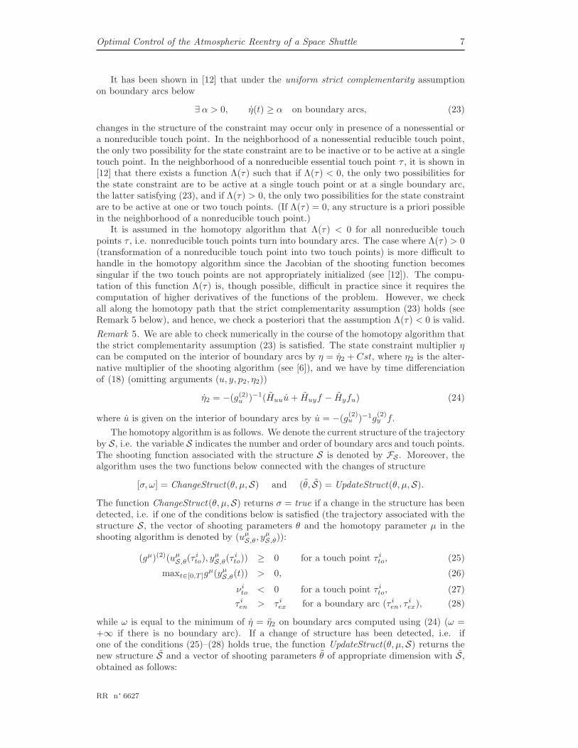
It has been shown in [12] that under the uniform strict complementarity assumptionon boundary arcs below

∃ α > 0, η(t) ≥ α on boundary arcs, (23)

changes in the structure of the constraint may occur only in presence of a nonessential ora nonreducible touch point. In the neighborhood of a nonessential reducible touch point,the only two possibility for the state constraint are to be inactive or to be active at a singletouch point. In the neighborhood of a nonreducible essential touch point τ , it is shown in[12] that there exists a function Λ(τ) such that if Λ(τ) < 0, the only two possibilities forthe state constraint are to be active at a single touch point or at a single boundary arc,the latter satisfying (23), and if Λ(τ) > 0, the only two possibilities for the state constraintare to be active at one or two touch points. (If Λ(τ) = 0, any structure is a priori possiblein the neighborhood of a nonreducible touch point.)

It is assumed in the homotopy algorithm that Λ(τ) < 0 for all nonreducible touchpoints τ , i.e. nonreducible touch points turn into boundary arcs. The case where Λ(τ) > 0(transformation of a nonreducible touch point into two touch points) is more difficult tohandle in the homotopy algorithm since the Jacobian of the shooting function becomessingular if the two touch points are not appropriately initialized (see [12]). The compu-tation of this function Λ(τ) is, though possible, difficult in practice since it requires thecomputation of higher derivatives of the functions of the problem. However, we checkall along the homotopy path that the strict complementarity assumption (23) holds (seeRemark 5 below), and hence, we check a posteriori that the assumption Λ(τ) < 0 is valid.

Remark 5. We are able to check numerically in the course of the homotopy algorithm thatthe strict complementarity assumption (23) is satisfied. The state constraint multiplier ηcan be computed on the interior of boundary arcs by η = η2 + Cst, where η2 is the alter-native multiplier of the shooting algorithm (see [6]), and we have by time differenciationof (18) (omitting arguments (u, y, p2, η2))

η2 = −(g(2)u )−1(Huuu+ Huyf − Hyfu) (24)

where u is given on the interior of boundary arcs by u = −(g(2)u )−1g

(2)y f.

The homotopy algorithm is as follows. We denote the current structure of the trajectoryby S, i.e. the variable S indicates the number and order of boundary arcs and touch points.The shooting function associated with the structure S is denoted by FS . Moreover, thealgorithm uses the two functions below connected with the changes of structure

[σ, ω] = ChangeStruct(θ, µ,S) and (θ, S) = UpdateStruct(θ, µ,S).

The function ChangeStruct(θ, µ,S) returns σ = true if a change in the structure has beendetected, i.e. if one of the conditions below is satisfied (the trajectory associated with thestructure S, the vector of shooting parameters θ and the homotopy parameter µ in theshooting algorithm is denoted by (uµ

S,θ, yµS,θ)):

(gµ)(2)(uµS,θ(τ

ito), y

µS,θ(τ

ito)) ≥ 0 for a touch point τ i

to, (25)

maxt∈[0,T ]gµ(yµ

S,θ(t)) > 0, (26)

νito < 0 for a touch point τ i

to, (27)

τ ien > τ i

ex for a boundary arc (τ ien, τ

iex), (28)

while ω is equal to the minimum of η = η2 on boundary arcs computed using (24) (ω =+∞ if there is no boundary arc). If a change of structure has been detected, i.e. ifone of the conditions (25)–(28) holds true, the function UpdateStruct(θ, µ,S) returns thenew structure S and a vector of shooting parameters θ of appropriate dimension with S,obtained as follows:

RR n° 6627

8 A. Hermant If (25) holds, then S is obtained from S by replacing the touch point τ ito by a boundary

arc, and θ is obtained from θ by replacing the touch point τ ito and its associated

shooting parameters νito and (yi

to, pito) by a boundary arc, with associated shooting

parameters

τ ien := τ i

to =: τ iex, ν1,i

en := νito, ν2,i

en := 0,

(yien, p

ien) := (yi

to, pito) =: (yi

ex, piex). If (26) holds and (25) does not, set τ := argmaxt∈[0,T ] g

µ(yµS,θ(t)). Then S is obtained

from S by adding the new touch point τ and θ is obtained from θ by adding the touchpoint τ i

to := τ , a zero jump parameter νito := 0 and the state-costate value at touch

point (yito, p

ito) := (yµ

S,θ(τ), pµS,θ(τ)). If (27) holds, then S is obtained from S by deleting the touch point τ i

to, and θ isobtained from θ by deleting the touch point τ i

to, its jump parameter νito and its

associated state-costate value (yito, p

ito). If (28) holds, then S is obtained from S by replacing the boundary arc (τ i

en, τiex) by

a touch point, and θ is obtained from θ by replacing the shooting parameters asso-ciated with the boundary arc (τ i

en, τiex) by a touch point and its associated shooting

parameters:

τ ito := τ i

en, νito := ν1,i

en , (yito, p

ito) := (yi

en, pien).

Finally, the function θ = Shooting(θ0, µ,FS) returns, if succeeds, a vector θ solution ofFS(θ, µ) = 0 obtained e.g. by a Newton algorithm initialized by the value θ0. Combininga classical predictor-corrector algorithm (see [1]) with the changes of structure describedabove, we obtain Algorithm 1.

The algorithm ends either because µ = 1 (success), or because the homotopy steplengthδ has been too much reduced (failure), or because ω ≤ 0 (the strict complementarityassumption on boundary arcs (23) fails).

The steplength δ is reduced either when the prediction is judged too bad, or when thecorrection fails, or at change of structure of the trajectory if the algorithm fails to initializea vector of shooting parameters for the new structure or does not find the new structure.It is increased after a successfull predictor-corrector step, so that the algorithm adjustsitself the homotopy steplength.

The complementarity condition on boundary arcs fails if a change of structure occursthat was not anticipated by the algorithm. This can happen e.g. if a boundary arc splitsinto two boundary arcs, or if the function Λ(τ) is positive at a nonreducible touch point τ(transformation of a touch point into two touch points). Otherwise, it has been shown in[12] that when Λ(τ) < 0, the uniform strict complementarity holds on emerging boundaryarcs.

It was shown in [12] that under some assumptions, this algorithm succeeds in reachingµ = 1. It is assumed in particular that only one change in the structure occur at a time.

Remark 6. No constraints on the initial and final state were considered in [12], but theresults can be extended if a strong controllability condition is assumed (see [4, section 8]).This condition means that the constraints (2)–(4) are jointly onto.

3 Model of atmospheric reentry

3.1 The optimal control problem

We use the model of atmospheric reentry of [9], to which we refer for further details. Letus recall that the state is composed of six variables, the radius r, velocity v, flight path

INRIA


Algorithm 1 Homotopy Algorithm

Input - θ0 = (y0, p0, λ, tf ) initial vector of shooting parameters for the unconstrainedproblem,- 0 < δmin < δ < δmax, minimum, current, and maximum values for the homotopysteplength,- distmax > 0 maximal distance to the curve FS(θ, µ) = 0 allowed in the predictionstep.

(Initialization) S := the empty structure (no boundary arc and no touch point),θ := Shooting(θ0, 1,FS) (assumed not to fail for good enough initial guess θ0),M := maxt∈[0,T ] g(y

1S,θ

(t)) (assumed to be positive),µ := 0, ω := +∞.

while µ < 1 and δ > δmin and ω > 0 do(Prediction step) Set µ := minµ+ δ; 1 and compute θ solution of

DθFS(θ, µ)(θ − θ) +DµFS(θ, µ)δ = 0.

if |FS(θ, µ)| > distmax then δ := δ/2

else (Correction Step) try θ = Shooting(θ, µ,FS)if fails then δ := δ/2else [σ, ω] := ChangeStruct(θ, µ,S)

if σ is true then (Change of structure)

(θ, S) := UpdateStruct(θ, µ,S)

try θ := Shooting(θ, µ,FS)

if fails then δ := δ/2

else [σ, ω] := ChangeStruct(θ, µ, S)if σ is true then δ := δ/2

else θ := θ, µ := µ, S := Send if

end ifelse (no change of structure) θ := θ, µ := µ, δ := min(2δ, δmax)end if

end ifend if

end while

RR n° 6627

10 A. Hermant

angle γ, latitude L, longitude l, and azimuth χ. The control is the bank angle β (the angleof attack is fixed following a given incidence profile, see [9, p.135]). The dynamics writes:

r = v sin γ, (29)

v = −g sinγ − SCD

2mρv2 + Ω2r cosL(sin γ cosL− cos γ sinL cosχ), (30)

γ = (−gv

+v

r) cos γ +

SCL

2mρv cosβ + 2Ω cosL sinχ

+ Ω2 r

vcosL(cos γ cosL+ sin γ sinL cosχ), (31)

L =v

rcos γ cosχ, (32)

l =v

r

cos γ sinχ

cosL, (33)

χ =SCL

2mρ

v

cos γsinβ +

v

rcos γ tanL sinχ+ 2Ω(sinL− tan γ cosL cosχ)

+ Ω2 r

v

sinL cosL sinχ

cos γ. (34)

The gravity g and atmospheric density ρ are modeled respectively by

g =g0r2

and ρ = ρ0e−(r−rE)

hs

where rE denotes the Earth radius and g0 and hs are positive constants whose numericalvalues can be found — as well as the other constants of the problem — in [9]. Theconstants S and m denote respectively the reference surface and mass of the shuttle, andΩ is the Earth rotation velocity. Here the (positive) aerodynamics coefficients CL and CD

are interpolated from the tabulated values of [9] as C3 functions (piecewise polynomials oforder 7) of r and v in order to satisfy assumption (A1).

The objective is to minimize the integral of the thermal flux, as in [7, 9]:

min

∫ tf

0

Cq

√ρv3dt (35)

where Cq > 0 is a fixed constant. The final time tf is free.Moreover, we consider the state constraint on the thermal flux, also considered in

[3, 7, 9, 13]:Φ = Cq

√ρv3 ≤ Φmax (36)

with Φmax = 7.4.105 W.m−2. (A different value Φmax = 7.173.105 W.m−2 was consideredin [9]. We explain later in Rem. 11 why our homotopy algorithm does not allow us tosolve the problem for Φmax < 7.4.105.)

Finally, the problem is subject to the boundary conditions given in Table 1 ([9]).

Initial conditions Final conditionsAltitude h = r − rE 119.82 km 15 kmVelocity v 7404.95 m.s−1 445 m.s−1

Flight angle γ -1.84 ° freeLatitude L 0 10.99 °Longitude l free 166.48°Azimuth χ free free.

Table 1: Boundary conditions

INRIA


Remark 7. It can be seen that the right-hand side of the dynamics (29)–(34) does notdepends on the longitude l, which does not appear in the cost (35) nor in the constraint(36). Since the initial longitude is free, the variable l can be omitted and computedafterwards once the optimal trajectory has been obtained by integrating backwards (33)from its final value ltf

= 166.48 prescribed in Table 1 (see [9]).

In what follows, we denote by y = (r, v, γ, L, χ) the state variable and by u or β thescalar control.

3.2 Assumptions

In order to apply the homotopy algorithm of [12], it is required that assumptions (A1)–(A3) hold. Assumption (A1) is satisfied by our model, and we will discuss in this sectionthe validity of assumptions (A2) and (A3).

Regularity of the Hamiltonian Let (u, y) denote an optimal trajectory. We have that

Hu = −pγ

SCL

2mρv sinβ + pχ

SCL

2mρ

v

cosγcosβ

where H denotes the generalized Hamiltonian (7). Let us assume that (this will be checkedin the numerical simulation)

Assumption (H0) In the flight domain, cos γ > 0.

If pγ and pχ do not vanish together, the (unique modulo 2π) control β minimizing theHamiltonian over U = R, i.e. satisfying (10), is given by

cosβ = − cos γpγ√

cos γ2p2γ + p2

χ

, sinβ = − pχ√

cos γ2p2γ + p2

χ

. (37)

(The control β is not uniquely determined, but since it is involved in the equations ofthe problem only by its sine and cosine, it is sufficient that the two above quantities areuniquely defined). However, because of our final boundary conditions and the transver-sality condition (12), we have that pγ(tf ) = pχ(tf ) = 0. We shall make the assumptionbelow:

Assumption (H1) For all t ∈ [0, tf ), either pγ(t) 6= 0 or pχ(t) 6= 0.

This assumption will be checked numerically since, as we will see, we have pχ(t) < 0 on(0, tf ) and pγ(0) 6= 0 (see Fig. 2(b) to 5(b)).

Lemma 8. Let (u, y) be a Pontryagin extremal. If assumption (H0)–(H1) hold, then u iscontinuous over [0, tf).

Proof. On [0, tf), the control u that minimizes the Hamiltonian is given by (37). Since thestate constraint (36) does not depend on γ nor on χ, the associated costate components,respectively pγ and pχ, are continuous over [0, tf ] by (9). The result follows.

Under assumptions (H0)–(H1), the control β can be computed as a smooth functionof the state and costate by (37) on [0, tf ). Moreover, at the minimizing control (37), wehave that

Huu = Huu =SCL

2mρ

v

cos γ

√

cos γ2p2γ + p2

χ. (38)

Therefore, the strenghtened Legendre-Clebsch condition (14) holds on [0, tf − ε] for everyε > 0, i.e. for every ε > 0 there exists α > 0 such that Huu ≥ α on [0, tf − ε]. Sincethe state constraint is not active at final time tf , the homotopy algorithm 1 is valid todetect the structure of the trajectory as long as assumption (H1) remains satisfied (seeRemark 11).

RR n° 6627

12 A. Hermant

Regularity of the state constraint The constraint on the thermal flux (36) is asecond-order state constraint. The second-order time derivative of the state constraint isgiven by

g(2) = A+B cosβ + C sinβ

where A = A(y), B = B(y), and C = C(y) are functions of the state and can be computedeither by hand or using formal calculus (see [9, p.122]). If 0 < B2 +C2 and A2 ≤ B2 +C2,the control on boundary arcs can be computed by

cosβ =−AB + σC

√B2 + C2 −A2

B2 + C2, sinβ =

−AC − σB√B2 + C2 −A2

B2 + C2, σ ∈ −1, 1.

The solution with σ = 1 is convenient in order to have a continuous control, which is anecessary optimality condition by Lemma 8. Moreover, we have that

g(2)u = σ

√

B2 + C2 −A2.

We shall therefore make the assumption below, which will be checked in the numericalsimulations:

Assumption (H2) In the neighborhood of the contact set of the state constraint, wehave A2 < B2 + C2.

This assumption implies that (A3) holds.Finally, we will assume that the extremals of the problem are normal (p0 = 1).

4 Resolution of the unconstrained problem

In order to apply the homotopy algorithm, it is required that a sufficiently good initialguess for the initial costate of the unconstrained problem can be provided in order tomake the (simple) shooting algorithm converge. We detail in this section how we proceedto initialize the unconstrained problem.

4.1 Resolution of the reduced problem in dimension 3

If we neglect the Earth rotation, i.e. Ω = 0, then the problem reduces to a problem withonly three state variables y = (r, v, γ) and control u = cosβ ∈ U = [−1, 1] (see [10, 8]):

Minimize∫ tf

0 Cq√ρv3dt subject to the state equation

r = v sin γ, (39)

v = −g sin γ − SCD

2mρv2, (40)

γ = (−gv

+v

r) cos γ +

SCL

2mρvu. (41)

Moreover, the problem is subject to the boundary conditions for r, v and γ given in Table1.

It was shown in [10, 8] by a geometric analysis that the optimal trajectory for the abovereduced problem in dimension 3 is composed by an arc with u = −1 followed by an arcwith u = +1.

In order to obtain the solution of the reduced problem, we proceed as in [9] and in-troduce the switching time tswitch and the free final time tf . Given a couple (tswitch, tf ),starting from the initial conditions y0 = (r0, v0, γ0) of Table 1, we integrate (39)–(41) withthe control u = −1 on (0, tswitch) and u = +1 on (tswitch, tf ) and search for a solution(t∗switch, t

∗f ) that satisfies the final conditions r(tf ) = rtf

and v(tf ) = vtfof Table 1. In

INRIA


this way the optimal trajectory solution of the reduced problem in dimension 3 can beobtained without introducing the adjoint variables.

In order to determine the latter, we introduce the unknown initial costate p0 =(p0

r, p0v, p

0γ) = (pr(0), pv(0), pγ(0)). Since the Hamiltonian of the reduced problem H is

given by

H = pγ

SCL

2mρvu + a function of (y, p),

Pontryagin’s minimum principle (10) yields that

u(t) =

−1 if pγ(t) > 0+1 if pγ(t) < 0.

(42)

Since pγ is continuous, (42) together with (12) and Rem. 3 implies that the three followingnecessary conditions have to be satisfied:

pγ(t∗switch) = 0, pγ(t∗f ) = 0, H(u(0), y(0), p(0)) = 0. (43)

Since the initial state y0 is known, as well as u(0) = −1, the last condition allows us toexpress p0

γ in function of p0r and p0

v by

p0γ = −(Φ(y0) + p0

rfr(y0) + p0

vfv(y0))/fγ(u(0), y0).

By a shooting algorithm (initialized by zero), integrating the costate equations we easilyobtain initial values p0

r and p0v in order to satisfy the two first conditions of (43).

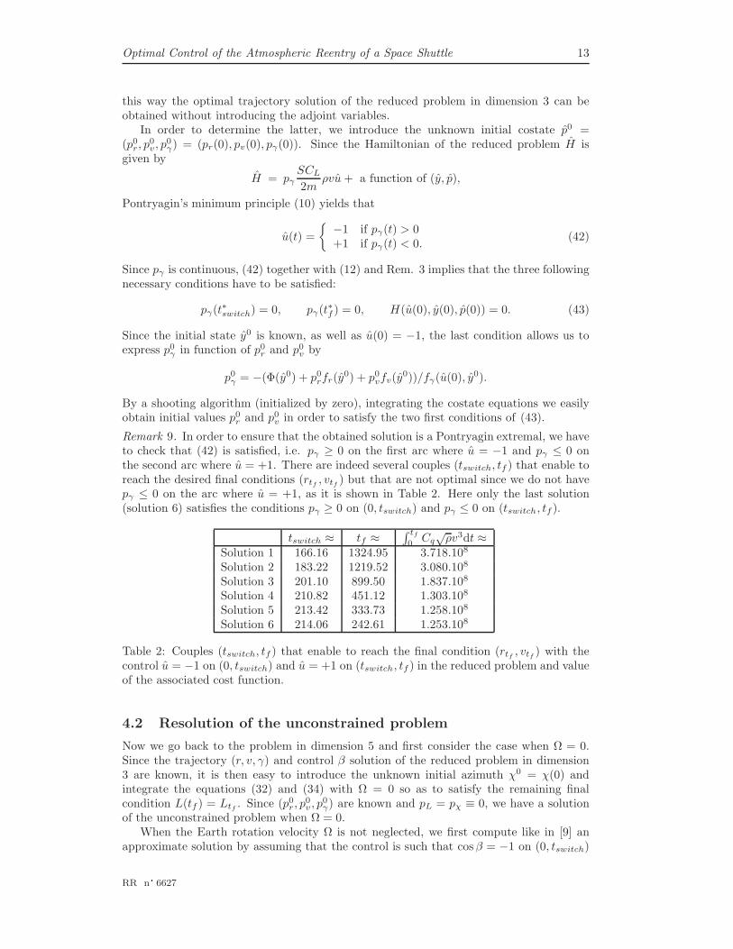
Remark 9. In order to ensure that the obtained solution is a Pontryagin extremal, we haveto check that (42) is satisfied, i.e. pγ ≥ 0 on the first arc where u = −1 and pγ ≤ 0 onthe second arc where u = +1. There are indeed several couples (tswitch, tf ) that enable toreach the desired final conditions (rtf

, vtf) but that are not optimal since we do not have

pγ ≤ 0 on the arc where u = +1, as it is shown in Table 2. Here only the last solution(solution 6) satisfies the conditions pγ ≥ 0 on (0, tswitch) and pγ ≤ 0 on (tswitch, tf ).

tswitch ≈ tf ≈∫ tf

0Cq

√ρv3dt ≈

Solution 1 166.16 1324.95 3.718.108

Solution 2 183.22 1219.52 3.080.108

Solution 3 201.10 899.50 1.837.108

Solution 4 210.82 451.12 1.303.108

Solution 5 213.42 333.73 1.258.108

Solution 6 214.06 242.61 1.253.108

Table 2: Couples (tswitch, tf ) that enable to reach the final condition (rtf, vtf

) with thecontrol u = −1 on (0, tswitch) and u = +1 on (tswitch, tf ) in the reduced problem and valueof the associated cost function.

4.2 Resolution of the unconstrained problem

Now we go back to the problem in dimension 5 and first consider the case when Ω = 0.Since the trajectory (r, v, γ) and control β solution of the reduced problem in dimension3 are known, it is then easy to introduce the unknown initial azimuth χ0 = χ(0) andintegrate the equations (32) and (34) with Ω = 0 so as to satisfy the remaining finalcondition L(tf ) = Ltf

. Since (p0r, p

0v, p

0γ) are known and pL = pχ ≡ 0, we have a solution

of the unconstrained problem when Ω = 0.When the Earth rotation velocity Ω is not neglected, we first compute like in [9] an

approximate solution by assuming that the control is such that cosβ = −1 on (0, tswitch)

RR n° 6627

14 A. Hermant

and cosβ = +1 on (tswitch, tf ). Here tswitch is a free parameter, as well as the final timetf . Using the values of parameters solutions of the problem with Ω = 0 as initial guess,we obtain a zero of the shooting function

χ0

p0r

p0v

p0γ

p0L

tswitch

tf

7→

H(u(0), y(0), p(0))r(tf ) − rtf

v(tf ) − vtf

L(tf ) − Ltf

pγ(tswitch)pγ(tf )pχ(tf )

(44)

where the state and costate equations are integrated with the control cosβ = −1 on(0, tswitch) and cosβ = +1 on (tswitch, tf). In this way we obtain a trajectory and costatesatisfying the state and costate equations (8)-(9) and transversality condition (12) as wellas (13). Only the minimum principle (10) is not satisfied.

Now we arrive to the last step of our initialization procedure. We consider the simpleshooting function

χ0

p0r

p0v

p0γ

p0L

tf

7→

H(u(0), y(0), p(0))r(tf ) − rtf

v(tf ) − vtf

L(tf ) − Ltf

pγ(tf )pχ(tf )

where the state and costate equations are integrated with the control β given as a functionof state and costate by (37). The value (χ0, p0

r, p0v, p

0γ , p

0L, tf ) previously obtained as a zero

of (44) provides a sufficiently good initial guess to make the simple shooting algorithmconverge, and we thus obtain a solution of the unconstrained problem, starting point ofthe homotopy algorithm. The solution and multipliers of the unconstrained problem areplotted in Fig. 2.

5 Resolution of the problem with state constraint

Now we have a solution of the problem without the state constraint, we apply the homotopyalgorithm 1 to our problem with the constraint (36) on the thermal flux. A sequence ofproblems (Pµ) for µ ∈ [0, 1] is solved, with state constraint

Φ = Cq

√ρv3 ≤ Φµ := µΦmax + (1 − µ)Φuncons

where Φuncons denotes the maximum of the thermal flux for the optimal solution of theunconstrained problem. We detail below the results of the algorithm.

5.1 Results

When the value of the homotopy parameter µ is increased from 0 to 1, the algorithmdetects three changes in the structure of the constraint detailed in Table 3.

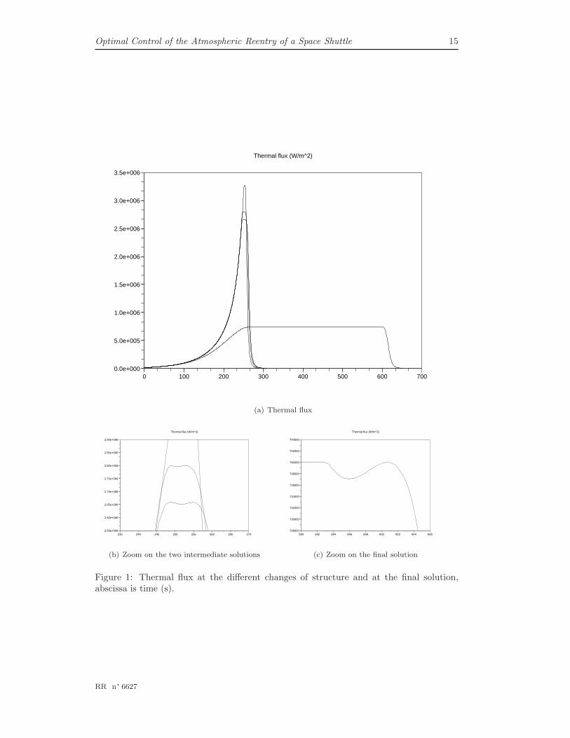
The thermal flux is plotted in Fig. 1 for the unconstrained problem, the final solutionand at two intermediate solutions when changes in the structure are detected: The firstone has a nonessential touch point and an essential one and the second has a nonreducibletouch point and a reducible one.

The state, control and multipliers associated with those four solutions are plotted inFig. 2 to 5.

INRIA


0 100 200 300 400 500 600 7000.0e+000

5.0e+005

1.0e+006

1.5e+006

2.0e+006

2.5e+006

3.0e+006

3.5e+006

Thermal flux (W/m^2)

(a) Thermal flux

235 240 245 250 255 260 265 2702.55e+006

2.60e+006

2.65e+006

2.70e+006

2.75e+006

2.80e+006

2.85e+006

2.90e+006


(b) Zoom on the two intermediate solutions

590 592 594 596 598 600 602 604 606728000

730000

732000

734000

736000

738000

740000

742000

744000


(c) Zoom on the final solution

Figure 1: Thermal flux at the different changes of structure and at the final solution,abscissa is time (s).

RR n° 6627

16 A. Hermant

0 50 100 150 200 250 3000

2e4

4e4

6e4

8e4

1e5

1.2e5

Altitude (m)

0 50 100 150 200 250 3000

1e3

2e3

3e3

4e3

5e3

6e3

7e3

8e3

Velocity (m/s)

0 50 100 150 200 250 300−1.0

−0.8

−0.6

−0.4

−0.2

0.0

0.2

0.4

0.6

Flight angle (rad)

0 50 100 150 200 250 3000.00

0.02

0.04

0.06

0.08

0.10

0.12

0.14

0.16

0.18

0.20

Latitude (rad)

0 50 100 150 200 250 3000.8

1.0

1.2

1.4

1.6

1.8

2.0

2.2

Azimuth (rad)

0 50 100 150 200 250 3000.0

0.5

1.0

1.5

2.0

2.5

3.0

3.5

Bank angle (rad)

(a) State and control

0 50 100 150 200 250 300−2e2

0

2e2

4e2

6e2

8e2

1e3

1.2e3

1.4e3

p_r

0 50 100 150 200 250 300−2e4

0

2e4

4e4

6e4

8e4

1e5

1.2e5

p_v

0 50 100 150 200 250 300−2e8

0

2e8

4e8

6e8

8e8

1e9

1.2e9

1.4e9

1.6e9

p_gamma

0 50 100 150 200 250 300

9.8e7

9.9e7

1e8

1.01e8

p_L

0 50 100 150 200 250 300−6e6

−5e6

−4e6

−3e6

−2e6

−1e6

0

p_chi

(b) Costate

Figure 2: Solution and multipliers of the unconstrained problem, abscissa is time (s).

INRIA


0 50 100 150 200 250 300 3500

2e4

4e4

6e4

8e4

1e5

1.2e5

Altitude (m)

0 50 100 150 200 250 300 3500

1e3

2e3

3e3

4e3

5e3

6e3

7e3

8e3

Velocity (m/s)

0 50 100 150 200 250 300 350−0.8

−0.6

−0.4

−0.2

0.0

0.2

0.4

Flight angle (rad)

0 50 100 150 200 250 300 3500.00

0.02

0.04

0.06

0.08

0.10

0.12

0.14

0.16

0.18

0.20

Latitude (rad)

0 50 100 150 200 250 300 3500.8

1.0

1.2

1.4

1.6

1.8

2.0

2.2

2.4

2.6

Azimuth (rad)

0 50 100 150 200 250 300 3500.0

0.5

1.0

1.5

2.0

2.5

3.0

3.5

Bank angle (rad)


0 50 100 150 200 250 300 350−2e3

−1.5e3

−1e3

−5e2

0

5e2

1e3

1.5e3

p_r

0 50 100 150 200 250 300 350−2e4

0

2e4

4e4

6e4

8e4

1e5

1.2e5

p_v

0 50 100 150 200 250 300 350−2e8

0

2e8

4e8

6e8

8e8

1e9

1.2e9

1.4e9

p_gamma

0 50 100 150 200 250 300 3508.4e7

8.5e7

8.6e7

8.7e7

p_L

0 50 100 150 200 250 300 350−5e6

−4.5e6

−4e6

−3.5e6

−3e6

−2.5e6

−2e6

−1.5e6

−1e6

−5e5

0

p_chi

0 50 100 150 200 250 300 350−14

−12

−10

−8

−6

−4

−2

0

eta

(b) Costate p and state constraint multiplier η

Figure 3: Solution and multipliers of the constrained problem with Φµ ≈ 2.65.106 W.m−2

(two touch points, the first one being nonessential), abscissa is time (s).

RR n° 6627

18 A. Hermant

0 50 100 150 200 250 300 3500

2e4

4e4

6e4

8e4

1e5

1.2e5

Altitude (m)

0 50 100 150 200 250 300 3500

1e3

2e3

3e3

4e3

5e3

6e3

7e3

8e3

Velocity (m/s)

0 50 100 150 200 250 300 350−0.8

−0.6

−0.4

−0.2

0.0

0.2

0.4

Flight angle (rad)

0 50 100 150 200 250 300 3500.00

0.02

0.04

0.06

0.08

0.10

0.12

0.14

0.16

0.18

0.20

Latitude (rad)

0 50 100 150 200 250 300 3500.8

1.0

1.2

1.4

1.6

1.8

2.0

2.2

2.4

2.6

Azimuth (rad)

0 50 100 150 200 250 300 3500.0

0.5

1.0

1.5

2.0

2.5

3.0

3.5

Bank angle (rad)


0 50 100 150 200 250 300 350−1.5e3

−1e3

−5e2

0

5e2

1e3

1.5e3

p_r

0 50 100 150 200 250 300 350−2e4

0

2e4

4e4

6e4

8e4

1e5

1.2e5

p_v

0 50 100 150 200 250 300 350−2e8

0

2e8

4e8

6e8

8e8

1e9

1.2e9

1.4e9

p_gamma

0 50 100 150 200 250 300 3508.1e7

8.2e7

8.3e7

8.4e7

p_L

0 50 100 150 200 250 300 350−5e6

−4e6

−3e6

−2e6

−1e6

0

1e6

p_chi

0 50 100 150 200 250 300 350−16

−14

−12

−10

−8

−6

−4

−2

0

eta

(b) Costate p and state constraint multiplier η

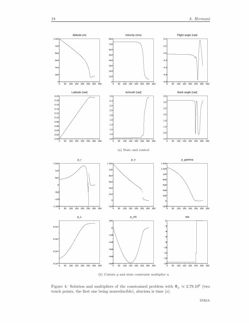
Figure 4: Solution and multipliers of the constrained problem with Φµ ≈ 2.79.106 (twotouch points, the first one being nonreducible), abscissa is time (s).

INRIA


0 100 200 300 400 500 600 7000

2e4

4e4

6e4

8e4

1e5

1.2e5

Altitude (m)

0 100 200 300 400 500 600 7000

1e3

2e3

3e3

4e3

5e3

6e3

7e3

8e3

Velocity (m/s)

0 100 200 300 400 500 600 700−1.0

−0.5

0.0

0.5

Flight angle (rad)

0 100 200 300 400 500 600 7000.00

0.02

0.04

0.06

0.08

0.10

0.12

0.14

0.16

0.18

0.20

Latitude (rad)

0 100 200 300 400 500 600 7001.1

1.2

1.3

1.4

1.5

1.6

1.7

1.8

1.9

Azimuth (rad)

0 100 200 300 400 500 600 7000.0

0.5

1.0

1.5

2.0

2.5

3.0

3.5

Bank angle (rad)


0 100 200 300 400 500 600 700−4e3

−2e3

0

2e3

4e3

6e3

8e3

p_r

0 100 200 300 400 500 600 7000

2e4

4e4

6e4

8e4

1e5

1.2e5

1.4e5

1.6e5

1.8e5

2e5

p_v

0 100 200 300 400 500 600 700−5e9

0

5e9

1e10

1.5e10

2e10

2.5e10

p_gamma

0 100 200 300 400 500 600 700−4e5

−2e5

0

2e5

4e5

6e5

8e5

p_L

0 100 200 300 400 500 600 700−1.6e6

−1.4e6

−1.2e6

−1.0e6

−8e5

−6e5

−4e5

−2e5

0

2e5

p_chi

0 100 200 300 400 500 600 700−400

−350

−300

−250

−200

−150

−100

−50

0

eta

(b) Alternative costate p2 and state constraint multiplier η

Figure 5: Solution and multipliers of the constrained problem with Φµ = 7.4.105 (oneboundary arc and one touch point), abscissa is time (s).

RR n° 6627

20 A. Hermant

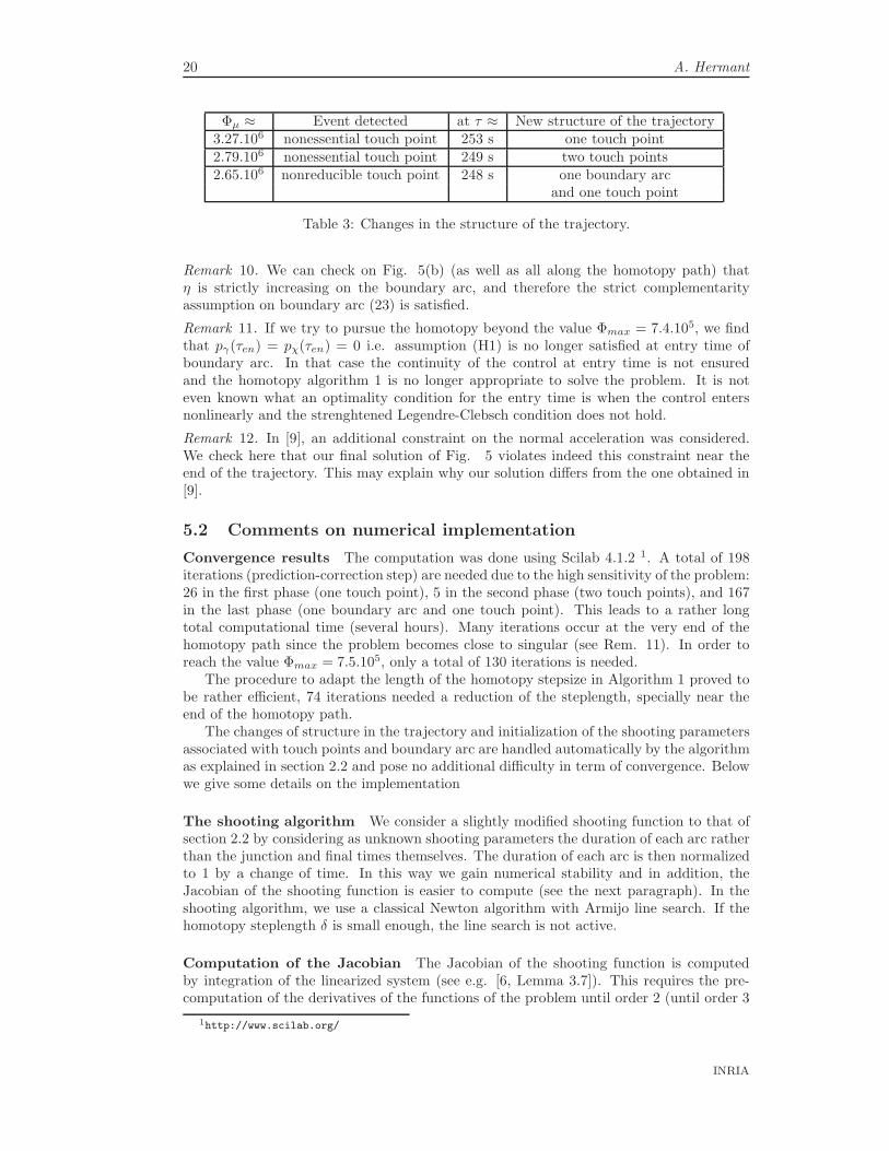
Φµ ≈ Event detected at τ ≈ New structure of the trajectory3.27.106 nonessential touch point 253 s one touch point2.79.106 nonessential touch point 249 s two touch points2.65.106 nonreducible touch point 248 s one boundary arc

and one touch point

Table 3: Changes in the structure of the trajectory.

Remark 10. We can check on Fig. 5(b) (as well as all along the homotopy path) thatη is strictly increasing on the boundary arc, and therefore the strict complementarityassumption on boundary arc (23) is satisfied.

Remark 11. If we try to pursue the homotopy beyond the value Φmax = 7.4.105, we findthat pγ(τen) = pχ(τen) = 0 i.e. assumption (H1) is no longer satisfied at entry time ofboundary arc. In that case the continuity of the control at entry time is not ensuredand the homotopy algorithm 1 is no longer appropriate to solve the problem. It is noteven known what an optimality condition for the entry time is when the control entersnonlinearly and the strenghtened Legendre-Clebsch condition does not hold.

Remark 12. In [9], an additional constraint on the normal acceleration was considered.We check here that our final solution of Fig. 5 violates indeed this constraint near theend of the trajectory. This may explain why our solution differs from the one obtained in[9].

5.2 Comments on numerical implementation

Convergence results The computation was done using Scilab 4.1.2 1. A total of 198iterations (prediction-correction step) are needed due to the high sensitivity of the problem:26 in the first phase (one touch point), 5 in the second phase (two touch points), and 167in the last phase (one boundary arc and one touch point). This leads to a rather longtotal computational time (several hours). Many iterations occur at the very end of thehomotopy path since the problem becomes close to singular (see Rem. 11). In order toreach the value Φmax = 7.5.105, only a total of 130 iterations is needed.

The procedure to adapt the length of the homotopy stepsize in Algorithm 1 proved tobe rather efficient, 74 iterations needed a reduction of the steplength, specially near theend of the homotopy path.

The changes of structure in the trajectory and initialization of the shooting parametersassociated with touch points and boundary arc are handled automatically by the algorithmas explained in section 2.2 and pose no additional difficulty in term of convergence. Belowwe give some details on the implementation

The shooting algorithm We consider a slightly modified shooting function to that ofsection 2.2 by considering as unknown shooting parameters the duration of each arc ratherthan the junction and final times themselves. The duration of each arc is then normalizedto 1 by a change of time. In this way we gain numerical stability and in addition, theJacobian of the shooting function is easier to compute (see the next paragraph). In theshooting algorithm, we use a classical Newton algorithm with Armijo line search. If thehomotopy steplength δ is small enough, the line search is not active.

Computation of the Jacobian The Jacobian of the shooting function is computedby integration of the linearized system (see e.g. [6, Lemma 3.7]). This requires the pre-computation of the derivatives of the functions of the problem until order 2 (until order 3

1http://www.scilab.org/

INRIA


for the state constraint), which has been done here by hands but can also be done usingformal calculus or automatic differentiation. This effort is rewarded by a better accuracy,improving the convergence of the shooting algorithm, and a gain in the computational time,both in the prediction and correction step, with comparison to a Jacobian computed byfinite differences (centered scheme). An accurate computation of the Jacobian is essentialto successfully follow the homotopy path.

Integrator An integrator with fixed step, Runge-Kutta of order 4, is used. This gives abetter convergence of the shooting algorithm than an integrator with a variable step. Thisseems to be due to the fact that the Jacobian of the shooting function can be computedmore accurately when the integration step is fixed.

Scaling and preconditioning It is known that in order to limit numerical errors, allthe state and costate variables have to be scaled in order to vary e.g. in the interval[−1, 1]. The jump parameters and duration of each arc have to be scaled as well. Thiscan be done by an efficient preconditioning of the Jacobian of the shooting function. Moreprecisely, in order to compute Newton’s direction in the shooting algorithm, instead ofsolving Ad = b where A := DθFS(θ, µ) and b := −FS(θ, µ), we set B := AD where D is a(given) diagonal matrix with i-th element dii = 10k if the i-th component of θ is of order

10k, solve Bd = b and then d := Dd. This simple manipulation considerably improve theconvergence of the shooting algorithm. Scaling and preconditioning have to be updated inthe course of the algorithm when the homotopy steplength becomes too small, speciallyin the last phase of the algorithm when the structure is composed of a boundary arc anda touch point. Finally, the use of QR-decompositions to solve the linear systems in theprediction and correction steps (see [1, Chapter 4]) is also an important factor to improvenumerical accuracy.

Acknoledgments The author is grateful to Pierre Martinon for helpful discussionsabout numerical homotopy methods and to Emmanuel Trelat for his remarks on the paper.

References

[1] E. L. Allgower and K. Georg. Introduction to numerical continuation methods, vol-ume 45 of Classics in Applied Mathematics. Society for Industrial and Applied Mathe-matics (SIAM), Philadelphia, PA, 2003. Reprint of the 1990 edition [Springer-Verlag,Berlin].

[2] P. Berkmann and H.J. Pesch. Abort landing in windshear: optimal control problemwith third-order state constraint and varied switching structure. J. of OptimizationTheory and Applications, 85, 1995.

[3] J.T. Betts. Practical methods for optimal control using nonlinear programming. Soci-ety for Industrial and Applied Mathematics (SIAM), Philadelphia, PA, 2001.

[4] J.F. Bonnans and A. Hermant. Second-order analysis for optimal control problemswith pure state constraints and mixed control-state constraints. INRIA ResearchReport 6199, to appear in Annales de l’Institut Henri Poincare (C) Analyse NonLineaire, doi:10.1016/j.anihpc.2007.12.002.

[5] J.F. Bonnans and A. Hermant. Stability and sensitivity analysis for optimal controlproblems with a first-order state constraint and application to continuation methods.ESAIM Control Optim. Calc. Var. (to appear), E-first DOI: 10.1051/cocv:2008016.

RR n° 6627

22 A. Hermant

[6] J.F. Bonnans and A. Hermant. Well-posedness of the shooting algorithm for stateconstrained optimal control problems with a single constraint and control. SIAM J.on Control and Optimization, 46(4):1398–1430, 2007.

[7] J.F. Bonnans and G. Launay. Large scale direct optimal control applied to a re-entryproblem. AIAA J. of Guidance, Control and Dynamics, 21:996–1000, 1998.

[8] B. Bonnard, L. Faubourg, G. Launay, and E. Trelat. Optimal control with stateconstraints and the space shuttle re-entry problem. J. Dynam. Control Systems,9(2):155–199, 2003.

[9] B. Bonnard, L. Faubourg, and E. Trelat. Optimal control of the atmospheric arc of aspace shuttle and numerical simulations with multiple-shooting method. MathematicalModels & Methods in Applied Sciences, 15(1):109–140, 2005.

[10] B. Bonnard and E. Trelat. Une approche geometrique du controle optimal de l’arcatmospherique de la navette spatiale. ESAIM: Control, Optimization and Calculus ofVariations, 7:179–222, 2002.

[11] R. Bulirsch, F. Montrone, and H. J. Pesch. Abort landing in the presence of windshearas a minimax optimal control problem. II. Multiple shooting and homotopy. J. Optim.Theory Appl., 70(2):223–254, 1991.

[12] A. Hermant. Homotopy algorithm for optimal control problems with a second-orderstate constraint. INRIA Research Report RR-6626, 2008. http://hal.inria.fr/inria-00316281/fr/.

[13] J. Laurent-Varin, F. Bonnans, N. Berend, M. Haddou, and C. Talbot. Interior-pointapproach to trajectory optimization. Journal of Guidance, Control, and Dynamics,30(5):1228–1238, 2007.

[14] K. Malanowski and H. Maurer. Sensitivity analysis for optimal control problemssubject to higher order state constraints. Annals of Operations Research, 101:43–73,2001. Optimization with data perturbations, II.

[15] H. J. Pesch. A practical guide to the solution of real-life optimal control problems.Control and Cybernetics, 23:7–60, 1994.

[16] H.J. Pesch. Real-time computation of feedback controls for constrained optimal con-trol problems. II. A correction method based on multiple shooting. Optimal ControlAppl. Methods, 10(2):147–171, 1989.

Contents

1 Introduction 3

2 Homotopy algorithm 42.1 General framework . . . . . . . . . . . . . . . . . . . . . . . . . . . . . . . . 42.2 Description of the homotopy algorithm . . . . . . . . . . . . . . . . . . . . . 5

3 Model of atmospheric reentry 83.1 The optimal control problem . . . . . . . . . . . . . . . . . . . . . . . . . . 83.2 Assumptions . . . . . . . . . . . . . . . . . . . . . . . . . . . . . . . . . . . 11

4 Resolution of the unconstrained problem 124.1 Resolution of the reduced problem in dimension 3 . . . . . . . . . . . . . . . 124.2 Resolution of the unconstrained problem . . . . . . . . . . . . . . . . . . . . 13

INRIA


5 Resolution of the problem with state constraint 145.1 Results . . . . . . . . . . . . . . . . . . . . . . . . . . . . . . . . . . . . . . . 145.2 Comments on numerical implementation . . . . . . . . . . . . . . . . . . . . 20

RR n° 6627

Centre de recherche INRIA Saclay – Île-de-FranceParc Orsay Université - ZAC des Vignes

4, rue Jacques Monod - 91893 Orsay Cedex (France)

Centre de recherche INRIA Bordeaux – Sud Ouest : Domaine Universitaire - 351, cours de la Libération - 33405 Talence CedexCentre de recherche INRIA Grenoble – Rhône-Alpes : 655, avenue de l’Europe - 38334 Montbonnot Saint-Ismier

Centre de recherche INRIA Lille – Nord Europe : Parc Scientifique de la Haute Borne - 40, avenue Halley - 59650 Villeneuve d’AscqCentre de recherche INRIA Nancy – Grand Est : LORIA, Technopôle de Nancy-Brabois - Campus scientifique

615, rue du Jardin Botanique - BP 101 - 54602 Villers-lès-Nancy CedexCentre de recherche INRIA Paris – Rocquencourt : Domaine de Voluceau - Rocquencourt - BP 105 - 78153 Le Chesnay CedexCentre de recherche INRIA Rennes – Bretagne Atlantique : IRISA, Campus universitaire de Beaulieu - 35042 Rennes Cedex

Centre de recherche INRIA Sophia Antipolis – Méditerranée :2004, route des Lucioles - BP 93 - 06902 Sophia Antipolis Cedex

ÉditeurINRIA - Domaine de Voluceau - Rocquencourt, BP 105 - 78153 Le Chesnay Cedex (France)http://www.inria.fr

ISSN 0249-6399

Documents

Optimal Control of the Atmospheric Reentry of a Space