University of Tennessee, Knoxville University of Tennessee, Knoxville

TRACE: Tennessee Research and Creative TRACE: Tennessee Research and Creative

Exchange Exchange

Masters Theses Graduate School

8-2013

Optimal Control of Differential Equations with Pure State Optimal Control of Differential Equations with Pure State

Constraints Constraints

Steven Lee Fassino University of Tennessee - Knoxville, sfassino@utk.edu

Follow this and additional works at: https://trace.tennessee.edu/utk_gradthes

Recommended Citation Recommended Citation Fassino, Steven Lee, "Optimal Control of Differential Equations with Pure State Constraints. " Master's Thesis, University of Tennessee, 2013. https://trace.tennessee.edu/utk_gradthes/2411

This Thesis is brought to you for free and open access by the Graduate School at TRACE: Tennessee Research and Creative Exchange. It has been accepted for inclusion in Masters Theses by an authorized administrator of TRACE: Tennessee Research and Creative Exchange. For more information, please contact trace@utk.edu.

To the Graduate Council:

I am submitting herewith a thesis written by Steven Lee Fassino entitled "Optimal Control of

Differential Equations with Pure State Constraints." I have examined the final electronic copy of

this thesis for form and content and recommend that it be accepted in partial fulfillment of the

requirements for the degree of Master of Science, with a major in Mathematics.

Suzanne Lenhart, Major Professor

We have read this thesis and recommend its acceptance:

Steven M. Wise, Charles Collins

Accepted for the Council:

Carolyn R. Hodges

Vice Provost and Dean of the Graduate School

(Original signatures are on file with official student records.)

University of Tennessee, KnoxvilleTrace: Tennessee Research and CreativeExchange

Masters Theses Graduate School

8-2013

Optimal Control of Differential Equations withPure State ConstraintsSteven Lee FassinoUniversity of Tennessee - Knoxville, sfassino@utk.edu

This Thesis is brought to you for free and open access by the Graduate School at Trace: Tennessee Research and Creative Exchange. It has beenaccepted for inclusion in Masters Theses by an authorized administrator of Trace: Tennessee Research and Creative Exchange. For more information,please contact trace@utk.edu.

To the Graduate Council:

I am submitting herewith a thesis written by Steven Lee Fassino entitled "Optimal Control of DifferentialEquations with Pure State Constraints." I have examined the final electronic copy of this thesis for formand content and recommend that it be accepted in partial fulfillment of the requirements for the degreeof Master of Science, with a major in Mathematics.

Suzanne Lenhart, Major Professor

We have read this thesis and recommend its acceptance:

Steve Wise, Charles Collins

Accepted for the Council:Carolyn R. Hodges

Vice Provost and Dean of the Graduate School

(Original signatures are on file with official student records.)

Optimal Control of Differential Equations

with Pure State Constraints

A Thesis Presented for the

Master of Science

Degree

The University of Tennessee, Knoxville

Steven Lee Fassino

August 2013

c© by Steven Lee Fassino, 2013

All Rights Reserved.

ii

To my family

iii

Acknowledgements

Many people are responsible for helping me through this journey, and I would like to express

my gratitude to those people. First and foremost, I would like to thank my advisor, Dr.

Suzanne Lenhart, for her incredible support and dedication over the years. Her contributions

to my fulfilling experiences as a student, researcher, and teacher are unmeasurable.

I want to thank my thesis committee members: Dr. Charles Collins and Dr. Steve

Wise for their time and keen insight throughout my time at UT. I thank Dr. Collins for his

willingness to share mathematical and teaching advice. I further thank Dr. Wise for first

exposing me to applied math and for his efforts in building colleague camaraderie outside

of school.

I give special thanks to Dr. Anil Rao for his help acquiring and understanding his

optimal control software.

Also, I appreciate all my fellow classmates, officemates, and professors who have provided

many useful discussions and made my time at UT incredibly enjoyable. In particular I want

to convey my gratitude to: Tyler Massaro, Jeremy Auerbach, Eddie Tu, John Collins, Marco

Martinez, and Mike Kelly.

I am extremely grateful for the financial support I received from the Mathematics

Department at UT and the opportunity granted to me as a Teaching Assistant.

I thank my family for their endless love and support. Thank you mom, Debbie Fassino,

for your encouragement and enthusiasm, and dad, Gary Fassino, for sharing your beautiful

mind.

I express profound gratitude to my friends for giving me more than they know.

iv

Abstract

Our work stems from examining a mathematical model that uses ordinary differential

equations to describe the dynamics of running. Previous work determined the optimal

running strategy for how a runner should control his/her force to maximize the distance

run in a given time. Distance covered is determined by the runner’s velocity. The runner’s

velocity is subject to the state differential equations that are based on Newton’s Second Law

and general energy flux. For physical reasonableness, we must assume energy cannot be

non-negative, which is a pure state constraint. Thus we solve the optimal control problem

applied to running that involves differential equations with pure state constraints.

Before solving the runner problem with the pure state constraint, we start by solving

simpler problems through implementing both direct and indirect methods. Applying

optimal control theory, these methods append to the Hamiltonian a penalty function that

either multiplies the state constraint directly or indirectly. Some of our examples can

be solved explicitly by using optimal control techniques and solving ordinary differential

equations exactly. Regardless for all of our examples, we illustrate numerical solutions

approximating the optimality system.

When analyzing the runner problem and its state constraint, we vary the type of control

implemented. We first look at the problem with a linear dependence on the control. We

have difficulty achieving the singular interval and maintaining non-negativity of energy, thus

realizing the challenge of solving this problem. So we approximate the runner problem with

a small quadratic dependence on the control. In this case, to satisfy the energy constraint,

we first attempt to find the penalty function and then try placing a terminal condition on

the energy state. We show the numerical results for the optimality systems of the various

v

formulations of the runner problem. We conclude that the pure state constraint of energy

proves difficult to implement regardless the type of control.

vi

Table of Contents

1 Introduction 1

1.1 Aim . . . . . . . . . . . . . . . . . . . . . . . . . . . . . . . . . . . . . . . . 1

1.2 Optimal Control Theory . . . . . . . . . . . . . . . . . . . . . . . . . . . . . 2

1.3 Linear Dependence on the Control . . . . . . . . . . . . . . . . . . . . . . . 6

1.4 State Variable Constraints . . . . . . . . . . . . . . . . . . . . . . . . . . . . 8

1.5 Numerical Methods . . . . . . . . . . . . . . . . . . . . . . . . . . . . . . . . 10

2 Pure State Constraint Examples 12

2.1 Introduction . . . . . . . . . . . . . . . . . . . . . . . . . . . . . . . . . . . . 12

2.2 Example 1 . . . . . . . . . . . . . . . . . . . . . . . . . . . . . . . . . . . . . 14

2.3 Example 2 . . . . . . . . . . . . . . . . . . . . . . . . . . . . . . . . . . . . . 22

2.4 Solving state constraint problems indirectly . . . . . . . . . . . . . . . . . . 33

3 Runner Problem 40

3.1 Introduction . . . . . . . . . . . . . . . . . . . . . . . . . . . . . . . . . . . . 40

3.2 Background . . . . . . . . . . . . . . . . . . . . . . . . . . . . . . . . . . . . 42

3.3 Mathematical Model . . . . . . . . . . . . . . . . . . . . . . . . . . . . . . . 43

3.4 Linear Dependence on the Control . . . . . . . . . . . . . . . . . . . . . . . 46

3.5 Quadratic Dependence on the Control . . . . . . . . . . . . . . . . . . . . . 53

4 Alternative Optimization Approaches and Conclusions 57

4.1 GPOPS . . . . . . . . . . . . . . . . . . . . . . . . . . . . . . . . . . . . . . 57

4.2 Conclusions . . . . . . . . . . . . . . . . . . . . . . . . . . . . . . . . . . . . 64

4.3 Future work . . . . . . . . . . . . . . . . . . . . . . . . . . . . . . . . . . . . 65

vii

Bibliography 67

Vita 70

viii

List of Tables

2.1 Example 2 - Different sets of constant and initial condition values . . . . . . 27

3.1 Physiological Parameter Values . . . . . . . . . . . . . . . . . . . . . . . . . 46

4.1 Mesh refinement conditions . . . . . . . . . . . . . . . . . . . . . . . . . . . 58

ix

List of Figures

1.1 Types of optimal subarcs . . . . . . . . . . . . . . . . . . . . . . . . . . . . 10

2.1 Example 1- Display of state variable and constraint from the explicit solutions 20

2.2 Example 1-Display of the optimality system and penalty function from the

explicit solutions . . . . . . . . . . . . . . . . . . . . . . . . . . . . . . . . . 20

2.3 Example 1- Display of state solution and constraint using the F-B S method 21

2.4 Example 1-Solution to the optimality system and penalty function using the

F-B S method . . . . . . . . . . . . . . . . . . . . . . . . . . . . . . . . . . . 21

2.5 Example 2, Set 1- Display of approximated state solution and the state

constraints from the F-B S method . . . . . . . . . . . . . . . . . . . . . . . 29

2.6 Example 2, Set 1- Approximated solution to optimality system with no tight

state constraints from the F-B S method . . . . . . . . . . . . . . . . . . . . 29

2.7 Example 2, Set 1- Display of state solution and the state constraints from

the algebraic approximation method . . . . . . . . . . . . . . . . . . . . . . 30

2.8 Example 2, Set 1- Solution to optimality system with no tight state

constraints from the algebraic approximation method . . . . . . . . . . . . . 30

2.9 Example 2, Set 2- Display of approximated state solution with tight state

constraints from using the F-B S method . . . . . . . . . . . . . . . . . . . 31

2.10 Example 2, Set 2- Approximated solution to optimality system with tight

state constraints from the F-B S method . . . . . . . . . . . . . . . . . . . . 31

2.11 Example 2, Set 2- Display of state solution with tight state constraints from

the algebraic approximation method . . . . . . . . . . . . . . . . . . . . . . 32

x

2.12 Example 2, Set 2- Solution to optimality system with tight state constraints

from the algebraic approximation method . . . . . . . . . . . . . . . . . . . 32

2.13 Solution to Indirect example from explicit analytical results . . . . . . . . . 39

3.1 Runner problem with linear dependence on the control with no energy state

constraint . . . . . . . . . . . . . . . . . . . . . . . . . . . . . . . . . . . . . 48

3.2 Sensitivity of the control update in the runner problem . . . . . . . . . . . . 51

3.3 Sensitivity of the control update in the runner problem . . . . . . . . . . . . 51

3.4 Sensitivity of the control update in the runner problem . . . . . . . . . . . . 52

3.5 Sensitivity of the control update in the runner problem . . . . . . . . . . . . 52

3.6 Runner problem with quadratic dependence on the control without the

energy state constraint directly implemented . . . . . . . . . . . . . . . . . 55

3.7 Runner problem with quadratic dependence on the control and terminal

condition . . . . . . . . . . . . . . . . . . . . . . . . . . . . . . . . . . . . . 56

4.1 Example 1 - Solution to the state equation approximated by GPOPS . . . . 59

4.2 Example 1 - Solution to the control equation approximated by GPOPS . . . 59

4.3 Example 2, Set 2 - Solution to the state equation approximated by GPOPS 60

4.4 Example 1, Set 2 - Solution to the control equation approximated by GPOPS 60

4.5 Indirect method example - Solution to the state equation approximated by

GPOPS . . . . . . . . . . . . . . . . . . . . . . . . . . . . . . . . . . . . . . 62

4.6 Indirect method example- Solution to the control equation approximated by

GPOPS . . . . . . . . . . . . . . . . . . . . . . . . . . . . . . . . . . . . . . 62

4.7 Runner problem with linear dependence on the control approximated by

GPOPS that did not converge . . . . . . . . . . . . . . . . . . . . . . . . . . 63

4.8 Runner problem with quadratic dependence on the control approximated by

GPOPS that did not converge . . . . . . . . . . . . . . . . . . . . . . . . . . 63

xi

Chapter 1

Introduction

1.1 Aim

We are interested in controlling a dynamical system to achieve a specific result. A dynamical

system is a model that can exist in various states and changes over time. A dynamical

system can have a variety of forms, but we look at a dynamical system consisting of ordinary

differential equations. We let x(t) be the state variable of the system at time t ∈ [0, T ], e.q.,

amount of a natural resource. We assume control of the state in the system exists through

the control variable, u(t), of the system at time t ∈ [0, T ], e.q., conservation rate. Then the

state equation is a differential equation,

x′(t) = g(t, x(t), u(t)) (1.1)

with x(0) = x0, that explains the instantaneous rate of change in the state variable. Given

the initial value of the state variable and the control trajectory, values of the control for

all t ∈ [0, T ], we can integrate the state equation to obtain the state trajectory. We want

to choose the control trajectory so that the state and control trajectories maximize (or

minimize) the objective functional,

J(u) =

∫ T

0f(t, x(t), u(t))dt. (1.2)

1

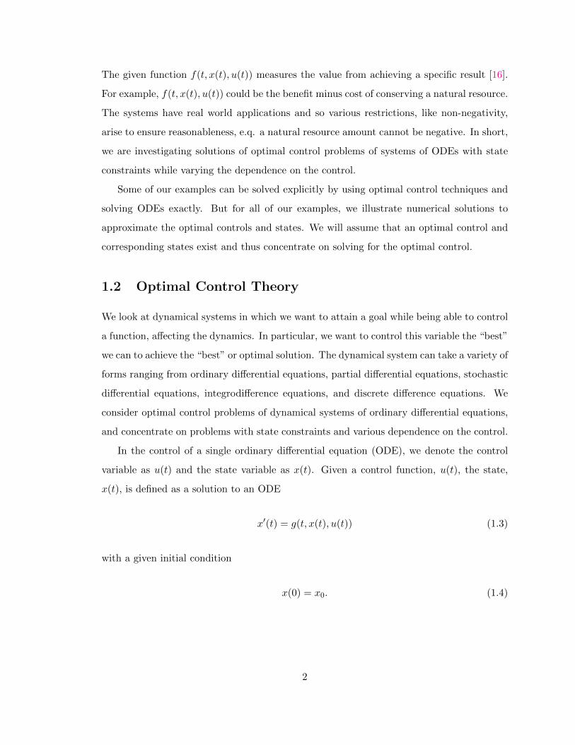
The given function f(t, x(t), u(t)) measures the value from achieving a specific result [16].

For example, f(t, x(t), u(t)) could be the benefit minus cost of conserving a natural resource.

The systems have real world applications and so various restrictions, like non-negativity,

arise to ensure reasonableness, e.q. a natural resource amount cannot be negative. In short,

we are investigating solutions of optimal control problems of systems of ODEs with state

constraints while varying the dependence on the control.

Some of our examples can be solved explicitly by using optimal control techniques and

solving ODEs exactly. But for all of our examples, we illustrate numerical solutions to

approximate the optimal controls and states. We will assume that an optimal control and

corresponding states exist and thus concentrate on solving for the optimal control.

1.2 Optimal Control Theory

We look at dynamical systems in which we want to attain a goal while being able to control

a function, affecting the dynamics. In particular, we want to control this variable the “best”

we can to achieve the “best” or optimal solution. The dynamical system can take a variety of

forms ranging from ordinary differential equations, partial differential equations, stochastic

differential equations, integrodifference equations, and discrete difference equations. We

consider optimal control problems of dynamical systems of ordinary differential equations,

and concentrate on problems with state constraints and various dependence on the control.

In the control of a single ordinary differential equation (ODE), we denote the control

variable as u(t) and the state variable as x(t). Given a control function, u(t), the state,

x(t), is defined as a solution to an ODE

x′(t) = g(t, x(t), u(t)) (1.3)

with a given initial condition

x(0) = x0. (1.4)

2

Note the rate of change of the state is dependent on the control variable u(t). Our goal is

expressed by the objective functional,

J(u) =

∫ T

0f(t, x(t), u(t))dt. (1.5)

We seek to find u∗(t) that achieves the maximum (or minimum) of our objective functional;

i.e., J(u∗) = maxu∈U J(u), where U is the set of possible controls. We will take U to be a

subset of piecewise-continuous functions. Also the objective functional is subject to (1.3)

and (1.4). The state and control variables usually both affect the goal.

The control that maximizes (or minimizes) the objective functional is denoted by

u∗(t). Substituting u∗(t) into the state differential equation (1.3) results in obtaining the

corresponding optimal state, x∗(t). Thus (u∗(t), x∗(t)) is the optimal pair.

In the 1950’s, Lev Pontryagin and his collaborators developed necessary conditions for

optimal control theory. If (u∗(t), x∗(t)) is an optimal pair, then these conditions hold.

From [10], Pontryagin introduced the idea of adjoint functions to append the differential

equations to the objective functional. These adjoint functions have a similar purpose as

Lagrange multipliers in multivariate calculus, which append constraints to the function of

several variables to be maximized or minimized. Refer to [10] for an introduction into

optimal control theory.

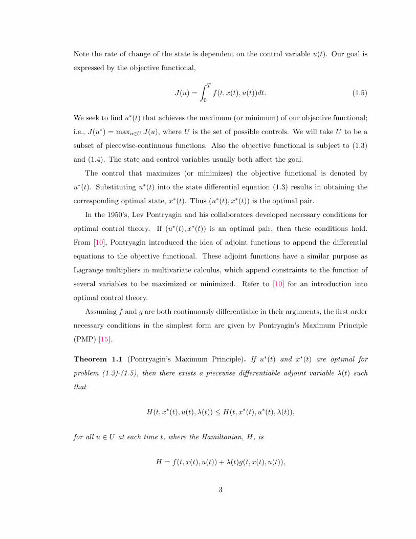
Assuming f and g are both continuously differentiable in their arguments, the first order

necessary conditions in the simplest form are given by Pontryagin’s Maximum Principle

(PMP) [15].

Theorem 1.1 (Pontryagin’s Maximum Principle). If u∗(t) and x∗(t) are optimal for

problem (1.3)-(1.5), then there exists a piecewise differentiable adjoint variable λ(t) such

that

H(t, x∗(t), u(t), λ(t)) ≤ H(t, x∗(t), u∗(t), λ(t)),

for all u ∈ U at each time t, where the Hamiltonian, H, is

H = f(t, x(t), u(t)) + λ(t)g(t, x(t), u(t)),

3

and

λ′(t) = −∂H(t, x∗(t), u∗(t), λ(t))

∂x,

λ(T ) = 0

Note the final time condition on the adjoint variable is called the transversality condition.

PMP changes the problem of finding the control that maximizes the objective functional

subject to the state ODE and initial condition to the problem of optimizing the Hamiltonian

pointwise. Another way to think of the Hamiltonian is

H =f(t, x(t), u(t)) + λ(t)g(t, x(t), u(t))

=(integrand) + (adjoint)× (RHS of ODE).

The necessary conditions can be generated by maximizing H with respect to u(t) at u∗(t).

From [10], they are as follows:

∂H

∂u= 0⇒ fu + λgu = 0 (optimality equation),

λ′ = −∂H∂x⇒ λ′ = −(fx + gx) (adjoint equation), and

λ(T ) = 0 (transversality condition).

We also consider second order conditions. For each t ∈ (0, T ), for a maximization

problem,

∂2H

∂u2≤ 0 at u∗(t)

must hold (from concavity), and for a minimization problem

∂2H

∂u2≥ 0 at u∗(t)

must hold (from convexity) [10].

4

Also, PMP can be extended to multiple states and controls and consequently corre-

sponding adjoint variables are introduced. For example, if we have n state variables,

x1(t) =g1(t, x1(t), ..., xn(t), u(t))

...

xn(t) =gn(t, x1(t), ..., xn(t), u(t)),

with corresponding initial conditions, then we introduce adjoint functions, λ1(t), ..., λn(t).

Thus the objective functional becomes,

maxu

∫ T

0f(t, x1(t), ..., xn(t), u(t))dt.

Similarly, the Hamiltonian is

H = f(t, x1(t), ..., xn(t), u(t)) + λ1(t)g1(t, x1(t), ..., xn(t), u(t))

+ ...

+ λn(t)(gn(t, x1(t), ..., xn(t), u(t))).

Accordingly the appropriate optimality equations, adjoint equations, and transversality

conditions are generated. For example, the i-th adjoint ODE is

λi = −∂H∂xi

. (1.6)

In short, for the simplest case we started with two unknowns, u∗(t) and x∗(t), and then

introduced an adjoint variable, λ(t). Thus we have to solve for three unknowns. We then

attain the optimality equation from setting

∂H

∂u

∣∣∣∣u=u∗

= 0 (1.7)

5

and solving for u∗(t), which will be characterized in terms of x∗(t) and λ(t). Note that

many real world application problems require bounds on the controls, like

a ≤ u(t) ≤ b

and that PMP still holds.

The optimality system is comprised of the state, adjoint ODEs and the control

characterization. Often solutions of the optimality system cannot be solved explicitly, but

can be approximated numerically. Refer to Section 1.5 for a summary of the numerical

methods used to solve optimality systems.

1.3 Linear Dependence on the Control

An optimal control problem with linear dependence on the control can be written as

maxu

∫ T

0[f1(t, x(t)) + f2(t, x(t))u(t)]dt (1.8)

subject to

x′(t) = g1(t, x(t)) + g2(t, x(t))u(t), (1.9)

and

umin ≤ u ≤ umax (1.10)

where

x(0) = x0. (1.11)

The Hamiltonian is

H = f1(t, x(t)) + λ(t)g1(t, x(t)) + [f2(t, x(t)) + λ(t)g2(t, x(t))]u(t). (1.12)

6

Since u(t) appears linearly in the Hamiltonian, we are unable to solve∂H

∂u= 0 for u(t).

The slope of H with respect to the control will help to determine the value of u∗ at time t.

Thus we define a switching function to be

ψ(t) =∂H

∂u= f2(t, x(t)) + λ(t)g2(t, x(t)). (1.13)

If we are solving a maximization problem, the optimal control takes the form:

u∗(t) =

umin, if ψ(t) < 0

∈ [umin, umax], if ψ(t) = 0

umax, if ψ(t) > 0.

(1.14)

Similarly, we reverse the optimal control values for a minimization problem. We split the

optimal control trajectory into three types of subarcs, when ψ(t) < 0, ψ(t) = 0, and

ψ(t) > 0. If ψ(t) only has isolated zeros, then the optimal control, u∗(t), switches values at

these zeros from umin to umax or vice versa. Thus the control is either at umax or umin over

[0, T ], which is referred to as a bang-bang control. If ψ(t) = 0 on some nontrivial subinterval

of time, then the optimal control is called singular on that interval. The times at which the

optimal control strategy switches from different subarcs are called junction times [16].

The Generalized Legendre-Clebsch condition (GLC) was developed as a necessary

condition for a singular control value to be optimal. Note H in this case trivially satisfies

the concavity requirement for a maximization problem. Thus, if u∗(t), x∗(t) are the optimal

pair on a singular subarc, then it is necessary that

(−1)k∂

∂u

[(∂

∂t

)2k ∂H

∂u

]≥ 0, (1.15)

holds for k = 0, 1, 2, ..., where k is the smallest positive integer such that the control

explicitly appears in

∂2kψ

∂t2k(1.16)

7

and the control does not appear in the lower derivatives [9, 2]. The dynamics of the specific

problem will give k exactly, and k is frequently 1.

1.4 State Variable Constraints

In application problems, state variables may be required to have specific bounds, like

being non-negative, for solutions to be reasonable. For more information regarding state

variable constraints refer to Chapter 2 and [16]. Let’s look at the following problem with

an inequality state constraint:

maxu

∫ T

0f(t, x, u)dt (1.17)

subject to

x′ = g(t, x, u) (1.18)

where

x(0) = x0 (1.19)

and the inequality state constraint

h(t, x) ≥ 0. (1.20)

As with optimal control problems we associate an adjoint function, λ, with the state

equation (1.18). Now we include a penalty multiplier function, η, to be associated with

the constraint (1.20), either directly or indirectly as noted in Section 2. For this example,

we directly adjoin the constraint and the penalty multiplier function, η(t), where η(t) is

defined as

η(t)h(t, x∗(t)) = 0 at x∗(t), (1.21)

8

meaning η ≡ 0 when h > 0, and η ≥ 0 otherwise. The Hamiltonian with appended penalty

function and constraint is

H = f(t, x, u) + λg(t, x, u) + η(t)h(t, x). (1.22)

When maximizing H with respect to the control u, it would not be advantageous for

h(t, x(t)) < 0 since that term would pull down H. Thus the penalty function helps to

maintain that h(t, x(t)) ≥ 0.

When solving a minimization problem, the penalty function is defined similarly to 1.21.

Still, η ≡ 0 when h > 0. However, η ≤ 0 when h is tight. Since, when minimizing H with

respect to the control u, violating the constraint would increase H and not be optimal since

η(t)h(t, x) > 0.

On the interior of the control set, the optimality condition takes the same form,

∂H

∂u= fu + λgu = 0. (1.23)

Interestingly, the adjoint DE becomes

λ′ = −∂H∂x

= −(fx + λgx + ηhx), (1.24)

which may help us solve for η(t) when h(t, x) = 0. Also the transversality condition is still,

λ(T ) = 0. (1.25)

So the value of the Hamiltonian and adjoint DE are only affected by η(t) when the constraint

is tight (h(t, x) = 0).

Investigating the possibility of a singular subarc, ψ(t) = 0, with the state constraint

yields two possible solutions, an interior subarc and boundary subarc. A solution is an

interior subarc if h > 0. A solution is a boundary subarc if h ≡ 0. In this case, since the

constraint is tight we find η(t) explicitly from differentiating ψ(t) = 0. Note that because

of the state constraint, the adjoint variable may be discontinuous [16]. See Figure 1.1 for

the possible subarcs that exist from a problem with linear dependence on the control.

9

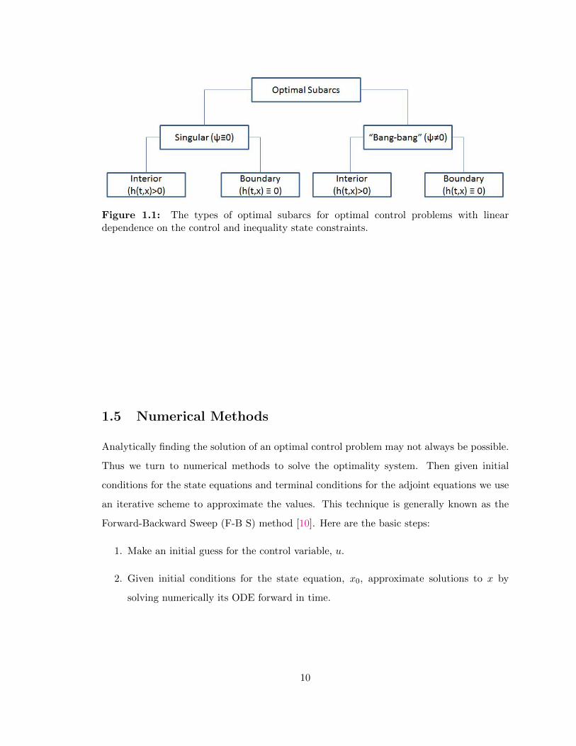
Figure 1.1: The types of optimal subarcs for optimal control problems with lineardependence on the control and inequality state constraints.

1.5 Numerical Methods

Analytically finding the solution of an optimal control problem may not always be possible.

Thus we turn to numerical methods to solve the optimality system. Then given initial

conditions for the state equations and terminal conditions for the adjoint equations we use

an iterative scheme to approximate the values. This technique is generally known as the

Forward-Backward Sweep (F-B S) method [10]. Here are the basic steps:

1. Make an initial guess for the control variable, u.

2. Given initial conditions for the state equation, x0, approximate solutions to x by

solving numerically its ODE forward in time.

10

3. Given the state solution from the previous step and the transversality condition,

λ(T ) = 0, approximate solutions to λ by solving numerically its ODE backwards in

time.

4. Update the value of the control with input from the new x and λ values by using a

convex combination of the previous control values and the current characterization of

u.

5. Check for convergence by repeating steps 1-4 until successive values of all state,

adjoint, and control functions are sufficiently close.

The last step for determining convergence requires the relative errors of the state,

adjoint, and control values from successive iterations to be less than a tolerance, δ. For

example,

‖uold − u‖‖u‖

≤ δ, (1.26)

must hold. This process generalizes to a state system of ODEs. Also, for a more in depth

description of this process refer to [10].

11

Chapter 2

Pure State Constraint Examples

2.1 Introduction

Often in real world problems, e.g. management science, economics, physical systems, there

are non-negativity constraints on the state variables, for example inventory levels, wealth,

or energy [16]. Non-negativity of the state equation requires

x(t) ≥ 0 for 0 ≤ t ≤ T. (2.1)

When such constraints do not include the control they are known as pure state variable

inequality constraints or pure state constraints. Pure state constraints are more difficult to

deal with than mixed state variable inequality constraints or mixed state constraints. Mixed

state constraints involve both the control and state variables. In a system with mixed state

constraints, since the control variable directly affects the constraint, one simply chooses the

appropriate control to satisfy the constraint. However, with pure state constraints, there

is no direct control of the control to ensure the constraint inequality is satisfied, so the

difficulty arises [16].

We define a pure state constraint mathematically as h(x, t) ≥ 0. We assume the function

h : En × E1 → Ep is continuously differentiable in all of its arguments. Note that h

represents a set of p constraints hi(t, x) ≥ 0, i = 1, 2, ..., p [16]. The constraint hi ≥ 0 is of

rth order if the rth time derivative of hi is the first time a term in control u appears in

the expression by putting g(t, x, u) in for x′ after each differentiation. Thus the control can

12

now be determined to satisfy the constraint hi ≥ 0. We only look at examples of first order

constraints, r = 1. Thus the first time derivative of h has terms in u, or

h1(t, x, u) =dh

dt=∂h

∂xg +

∂h

∂t. (2.2)

Most likely, the important special case of the non-negativity constraint, x(t) ≥ 0, for t ∈

[0, T ] will be of order one since g(t, x, u) typically has terms in u [16].

There are two ways to handle pure state constraints: direct and indirect methods. The

direct method appends to the Hamiltonian a penalty multiplier that directly multiplies the

constraint. The indirect method, appends to the Hamiltonian a similar penalty multiplier

that instead multiplies the first time derivative of the constraint. As [16] notes, “This

derivative will involve time derivatives of the state variables, which can be written in terms of

the control and state variables through the use of the state equations. Thus, the restrictions

on the time derivatives of the pure state constraints are transformed in the form of mixed

constraints.” For each method, if the problem has multiple constraints, then a penalty

multiplier exists for each constraint. Note that the adjoint functions may have jumps at

the junction times where the pure state constraints become tight [16].

In solving problems with pure state constraints, we refer to the Maximum Principle given

in [16], that has some additional conditions which must hold. The transversality condition

is λ(T−) = γhx(x∗(T ), T ) for γ ≥ 0. Also, jump conditions may exist on adjoint variable

at contact time τ , where the state trajectory enters or exits an arc where the constraint is

tight. In particular,

λ(τ−) = λ(τ+) + ζ(τ)hx(x∗(τ), τ) (2.3)

H[x∗(τ), u∗(τ−), λ(τ−), τ ] = H[x∗(τ), u∗(τ+), λ(τ+), τ ]− ζht(x∗(τ), τ), (2.4)

and ζ ≥ 0, ζ(τ)h(x∗(τ), τ) = 0 must hold.

State constraints are realistic restrictions imposed on a system, and thus we start with

solving both analytically and numerically a variety of problems involving them from [6].

We illustrate the technique of appending to the Hamiltonian a penalty multiplier function

13

that directly multiplies the pure state constraint. In the following examples we show the

analytical results first, then describe their numerical approaches and results.

2.2 Example 1

Solve

minu

∫ 5

0

(4x(t) + u(t)2

)dt, (2.5)

subject to

x′(t) = u(t) (2.6)

with the initial condition of x(0) = 10 and terminal condition of x(5) = 0. Also, we have

the inequality state constraint, h(t, x), that we define as

h(t, x) = x− (6− 2t) ≥ 0. (2.7)

Adding a penalty term that directly multiplies the state constraint to the Hamiltonian and

forces the optimal state to satisfy the state constraint is called the direct method.

Using Pontryagin’s Maximum Principle (PMP) and the direct method, the Hamiltonian

is

H = 4x+ u2 + λu+ η(x− (6− 2t)), (2.8)

where the penalty function, η(t) ≤ 0, satisfies η ≡ 0 when x(t) > 6−2t, and η ≤ 0 otherwise

when (2.7) is tight (i.e. x(t) = 6− 2t).

Since we seek to minimize H with respect to u, a state variable violating the constraint

would increase H and not be optimal since η(t)(x− (6− 2t)) > 0. Consider the derivative

of the Hamiltonian with respect to the control,

∂H

∂u= 2u+ λ. (2.9)

14

Since our control has no upper or lower bound constraints, we can directly consider the

optimality condition, u∗, from solving when (2.9) equals 0,

u∗ =−λ2. (2.10)

Note that

∂2H

∂u2= 2, (2.11)

which is the correct convexity for a minimization problem. The adjoint differential equation

is

λ′ =−∂H∂x

= −(4 + η) = −η − 4. (2.12)

No transversality condition exists on λ because of the terminal condition on x.

At the times when the constraint (2.7) is not tight, then η(t) = 0 and H = 4x+u2 +λu.

So,∂H

∂uis the same as (2.9), but λ′ = −4. Thus, x′ = u =

−λ2

implies

x′′ =−λ′

2= −(

−4

2) = 2. (2.13)

Solving that ODE, we know x′′ = 2, yields that x′ = 2t+ c1, and so x = t2 + c1t+ c2.

If the constraint is tight, then (2.8) and (2.10) apply and η may not be 0. So x(t) = 6−2t

implies x′ = −2. Since

x′ = u = −2 =−λ2, (2.14)

we have λ = 4, and λ′ = 0. Substituting this into the adjoint DE equation yields

λ′ = 0 = −η − 4

and

η = −4. (2.15)

15

Since at t = 0, x(0) > 6− 2(0), the constraint is not tight near t = 0.

If u = −2 on (0, t1), the solution is of the form

x = t2 + c1t+ c2. (2.16)

Then using the initial condition x(0) = c2 = 10 the solution becomes

x = t21 + c1t1 + 10, 0 ≤ t ≤ t1. (2.17)

At the intersection of the state trajectory and the constraint equations, (2.17) and (2.7),

t21 + c1t+ 10 = 6− 2t1. (2.18)

Continuity of the derivatives at this intersection implies

2t1 + c1 = −2 (2.19)

also holds.

We denote by t1 ≤ t ≤ t2, the interval when the state trajectory is on the constraint

curve, the solution is sliding down the constraint until some time t2. When t1 ≤ t ≤ t2, we

already know the solution from (2.7). Since x(5) = 0 > 6 − 2(5). The terminal condition

implies t2 < 5.

Let’s look at the state solution on the final interval, t2 ≤ t ≤ 5, which we know is of the

form

x = t2 + c3t+ c4. (2.20)

The terminal condition, x(5) = 0, gives us the solution

25 + 5c3 + c4 = 0 (2.21)

16

when t = 5. We look at the intersection of the constraint curve and the state solution when

(2.20)=(2.7),

6− 2t2 = t22 + c3t2 + c4. (2.22)

Then because of continuity of the derivatives at this intersection,

−2 = 2t2 + c3. (2.23)

We now have five equations, (2.18),(2.19),(2.21), (2.22), and (2.23) and five unknowns,

t1, t2, c1, c3, and c4.

We solve for and obtain t1 = 2, t2 = 3, c1 = −6, c2 = 10, c3 = −8, and c4 = 15. Note we

construct λ from the optimality condition (2.10),

u∗ = −λ/2⇒ λ = −2u∗. (2.24)

Putting all of these results together we conclude,

x∗(t) =

t2 − 6t+ 10, 0 ≤ t ≤ 2

6− 2t, 2 ≤ t ≤ 3

t2 − 8t+ 15, 3 ≤ t ≤ 5

(2.25)

u∗(t) =

2t− 6, 0 ≤ t ≤ 2

−2, 2 ≤ t ≤ 3

2t− 8, 3 ≤ t ≤ 5

(2.26)

17

λ(t) =

−4t+ 12, 0 ≤ t ≤ 2

4, 2 ≤ t ≤ 3

−4t+ 16, 3 ≤ t ≤ 5

(2.27)

η(t) =

0, 0 ≤ t ≤ 2

−4, 2 ≤ t ≤ 3

0, 3 ≤ t ≤ 5

(2.28)

This simple example allows us to find the solutions explicitly by hand, and we can

see the plots of the solutions to the optimality system and penalty function in Figure 2.1

and Figure 2.2 . Thus we implement this problem numerically using the forward-backward

sweep method and show the similar results in Figure 2.3 and Figure 2.4. Later we see how

this extends to more complex problems in Section 2.3 and Chapter 3.

Given the problem in (2.5) subject to (2.6), (2.7) and the given initial condition and

terminal condition we developed an iterative scheme similar to that in Section 1.5 to find

the solution of optimality system and the penalty multiplier η. For these simple ODEs,

we used Euler’s method with a ∆t = .005. We include an if-else loop in the adjoint

equation to define the η function depending on whether the constraint is tight or not. The

optimality condition is implemented directly and the value of the control is determined by

averaging the previous control value with the new control value from the characterization,

u = .5n ∗ unew + (1− .5n) ∗ uprev . Note that n is the iteration count and that more weight

is placed on the previous control than the new control. For convergence, relative error for

control, state, and adjoint values of successive iterations was used with a tolerance of 10−4.

Finding the correct λ value at the final time is a result of searching across a grid of values

for λ(5) and choosing the one for which the corresponding state satisfies x(5) = 0. We find

that λ(5) = −4.01 satisfies the terminal condition best with a value of x(5) = −0.0030,

which closely matches the explicit solution in (2.27).

18

Looking at the results from solving the optimality system numerically, we see in Figure

2.3 that the state solution hits the constraint at t = 2 and slides down until t = 3, at which

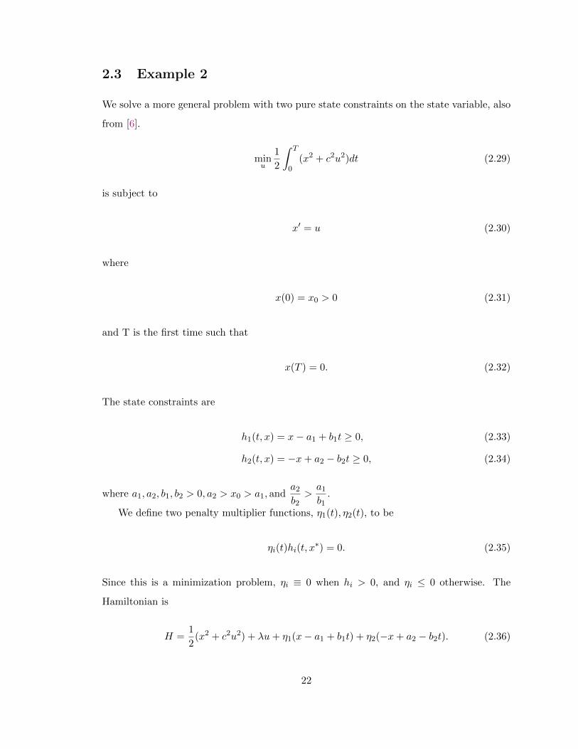
the solution goes towards the terminal condition x(5) = 0. From (2.28), we expect the η

function to be active from 2 ≤ t ≤ 3, and we see that in Figure 2.4. Similarly, Figure 2.4

shows the adjoint solution matching our findings from (2.27) and agrees with λ(5) = −4.

The value of the objective functional calculated from the explicit solution and F-B S method

is 82.666 and 82.740 respectively.

19

Figure 2.1: From the explicit solutions, a plot of the state variable with the inequalityconstraint shaded.

Figure 2.2: The solution for the state, control, λ, and η variables to Example 1 from theexplicit solutions.

20

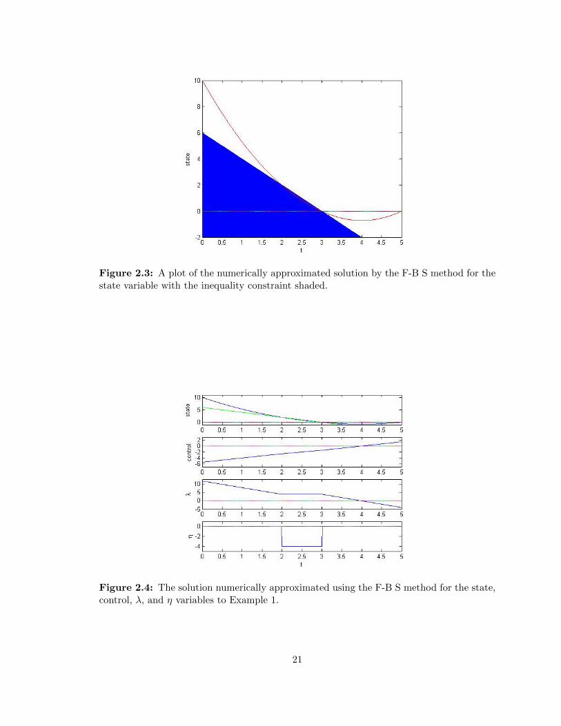
Figure 2.3: A plot of the numerically approximated solution by the F-B S method for thestate variable with the inequality constraint shaded.

Figure 2.4: The solution numerically approximated using the F-B S method for the state,control, λ, and η variables to Example 1.

21

2.3 Example 2

We solve a more general problem with two pure state constraints on the state variable, also

from [6].

minu

1

2

∫ T

0(x2 + c2u2)dt (2.29)

is subject to

x′ = u (2.30)

where

x(0) = x0 > 0 (2.31)

and T is the first time such that

x(T ) = 0. (2.32)

The state constraints are

h1(t, x) = x− a1 + b1t ≥ 0, (2.33)

h2(t, x) = −x+ a2 − b2t ≥ 0, (2.34)

where a1, a2, b1, b2 > 0, a2 > x0 > a1, anda2b2>a1b1

.

We define two penalty multiplier functions, η1(t), η2(t), to be

ηi(t)hi(t, x∗) = 0. (2.35)

Since this is a minimization problem, ηi ≡ 0 when hi > 0, and ηi ≤ 0 otherwise. The

Hamiltonian is

H =1

2(x2 + c2u2) + λu+ η1(x− a1 + b1t) + η2(−x+ a2 − b2t). (2.36)

22

Finding the optimality condition,

∂H

∂u= c2u+ λ = 0⇒ u∗ = − λ

c2. (2.37)

The adjoint is

λ′ = −(x+ η1 − η2) = −x− η1 + η2. (2.38)

No boundary conditions on λ occur because initial and terminal conditions for x are

given. Also, x(T ) = 0 paired with the constraints (2.33), (2.34) restrict our final T,

a1b1≤ T ≤ a2

b2. (2.39)

From a property of the transversality condition of the necessary conditions for solving

problems with terminal conditions given in [16], either

H(t) = 0 and a1/b1 < T < a2/b2, (2.40)

H(T ) ≥ 0 and T = a1/b1, (2.41)

H(T ) ≤ 0 and T = a2/b2. (2.42)

We next find the solution to decide which condition (2.40), (2.41), or (2.42) applies to our

problem. If both constraints (2.28), (2.29) are not tight, then

H =1

2(x2 + c2u2) + λu. (2.43)

Also,∂H

∂uis the same as (2.37) but λ′ = −x. Thus, x′ = u = − λ

c2implies

x′′ =x

c2> 0. (2.44)

Solving for the solution, we know it is of the form

x = k1et/c + k2e

−t/c (2.45)

23

for some constants, k1, k2.

At the final time, x(T ) = 0 means

H =1

2c2u2 + λu = −1

2

λ2

c2= −1

2c2u2 = 0, (2.46)

only if u(T ) = 0. Using this solution form, we know that

u(T ) = x′(T ) =k1ceT/c − k2

ce−T/c (2.47)

and

x(T ) = k1eT/c + k2e

−T/c = 0. (2.48)

Thus having both u(T ) = x(T ) = 0 implies k1 = k2 = 0, thus x(t) = 0 on a final free

interval. This contradicts property of T being first moment of x = 0, and so a constraint

must be tight at T . In particular, the constraint h2 will be tight and (2.41) is satisfied so

that T =a2b2

. Since H ≤ 0 at t = T and H = 0 at t = T leads to a contradiction.

As long as constraint h1 is not tight near t = 0 and right before t = T , the solution is

of the same form as (2.41) and satisfies

x(0) = k1 + k2 = x0, (2.49)

x(T ) = x(a2/b2) = k1ea2/b2c + k2e

−a2/b2c = 0. (2.50)

If one of the constraints are tight, then (2.36), (2.38) apply. Looking at h1 being tight

implies η2 = 0 and x(t) = a1 − b1t, thus x′ = −b1. Since

x′ = u = −b1 =−λc2

(2.51)

we know that λ is a constant. Substituting λ′ = 0 into the adjoint DE (2.38) yields

λ′ = 0 = −x− η1 ⇒ η1 = −x. (2.52)

24

Looking at h2 being tight implies η1 = 0 and x(t) = a2 − b2t, thus x′ = −b2. Since

x′ = u = −b2 =−λc2

(2.53)

we know that λ is a constant. Substituting λ′ = 0 into the adjoint DE (2.38) yields

λ′ = 0 = −x+ η2 ⇒ η2 = x. (2.54)

Since x is convex during the trajectory, it cannot be tangent to the h2 constraint in

(2.34). We know the solution only hits h2 at T from (2.42), thus only possibility of constraint

being tight is h1. So the solution will take the form of (2.45) from (0, t1) to a point of

tangency with h1 = 0 from (t1, t2). The solution will slide down the h1 = 0 constraint until

time t2 at which the solution will take the form of (2.45) from (t2, a2/b2). Defined succinctly

the solution is

x∗(t) =

k1e

t/c + k2e−t/c, 0 ≤ t ≤ t1

a1 − b1t, t1 ≤ t ≤ t2

k3et/c + k4e

−t/c, t2 ≤ t ≤ a2/b2,

(2.55)

where the values of k1, k2, and junction time t1 are determined by the initial condition and

the properties of continuity and tangency at t1. Specifically we use (2.31),

k1et1/c + k2e

−t1/c = a1 − b1t1, (2.56)

and

k1cet1/c − k2

ce−t1/c = −b1. (2.57)

The values of k3, k4, and junction time t2 are determined by the terminal condition and

the properties of continuity and tangency at t2. Specifically we use (2.32),

k3et2/c + k4e

−t2/c = a1 − b1t2, (2.58)

25

and

k3cet2/c − k4

ce−t2/c = −b1. (2.59)

Upon finding those constants and junction times, we construct and conclude:

u∗(t) =

k1cet/c − k2

ce−t/c, 0 ≤ t ≤ t1

−b1, t1 ≤ t ≤ t2k3cet/c − k4

ce−t/c, t2 ≤ t ≤ a2/b2

(2.60)

λ(t) =

−c2(k1

cet/c − k2

ce−t/c), 0 ≤ t ≤ t1

b1c2, t1 ≤ t ≤ t2

−c2(k3cet/c − k4

ce−t/c), t2 ≤ t ≤ a2/b2

(2.61)

η1(t) =

0, 0 ≤ t ≤ t1

−x, t1 ≤ t ≤ t2

0, t2 ≤ t ≤ a2/b2

(2.62)

We solve this more general problem numerically through defining the various constants,

a1, a2, b1, b2, c and the initial condition, x0. We will show the solutions to the optimality set

and penalty function for two different sets of defined constants and initial conditions. The

first set demonstrates what happens when the constraint (2.33) is not tight. The second

shows us what happens when the constraint (2.33) is tight and thus the penalty multiplier

is active.

For both sets of constants and initial conditions, given the problem in (2.29) subject

to (2.30), (2.31), (2.32), (2.33), and (2.34), we used an iterative scheme similar to that in

Section 1.5 to find the solution of optimality system and the penalty multiplier η. We apply

the forward-backward sweep method, (F-B S), to solve for the state and adjoint equations.

26

Similarly for convergence, relative error with a tolerance of 10−3 is used. The specifics of the

method and techniques are the same as in Example 1. Finding the correct λ(T ) is a result

of searching across a grid of possible values and choosing the one which satisfies x(T ) = 0.

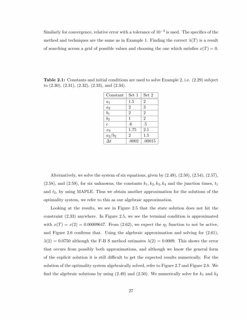
Table 2.1: Constants and initial conditions are used to solve Example 2, i.e. (2.29) subjectto (2.30), (2.31), (2.32), (2.33), and (2.34).

Constant Set 1 Set 2

a1 1.5 2

a2 2 3

b1 2 2

b2 1 2

c .6 .5

x0 1.75 2.1

a2/b2 2 1.5

∆t .0002 .00015

Alternatively, we solve the system of six equations, given by (2.49), (2.50), (2.54), (2.57),

(2.58), and (2.59), for six unknowns, the constants k1, k2, k3, k4 and the junction times, t1

and t2, by using MAPLE. Thus we obtain another approximation for the solutions of the

optimality system, we refer to this as our algebraic approximation.

Looking at the results, we see in Figure 2.5 that the state solution does not hit the

constraint (2.33) anywhere. In Figure 2.5, we see the terminal condition is approximated

with x(T ) = x(2) = 0.00009647. From (2.62), we expect the η1 function to not be active,

and Figure 2.6 confirms that. Using the algebraic approximation and solving for (2.61),

λ(2) = 0.0750 although the F-B S method estimates λ(2) = 0.0009. This shows the error

that occurs from possibly both approximations, and although we know the general form

of the explicit solution it is still difficult to get the expected results numerically. For the

solution of the optimality system algebraically solved, refer to Figure 2.7 and Figure 2.8. We

find the algebraic solutions by using (2.49) and (2.50). We numerically solve for k1 and k2

27

in MAPLE and build the system of solutions shown in Figure 2.8 from (2.45). Note for the

algebraically approximated solutions to Set 1, we find k1 = −0.002229 and k2 = 1.7522299.

28

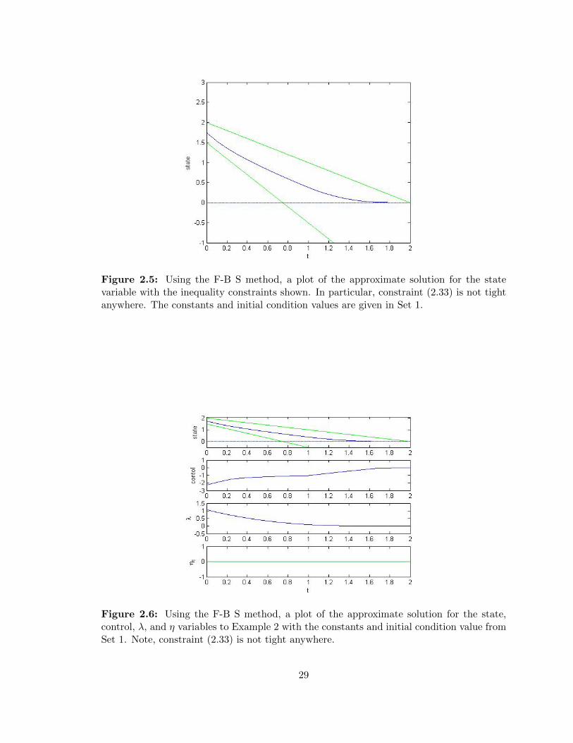
Figure 2.5: Using the F-B S method, a plot of the approximate solution for the statevariable with the inequality constraints shown. In particular, constraint (2.33) is not tightanywhere. The constants and initial condition values are given in Set 1.

Figure 2.6: Using the F-B S method, a plot of the approximate solution for the state,control, λ, and η variables to Example 2 with the constants and initial condition value fromSet 1. Note, constraint (2.33) is not tight anywhere.

29

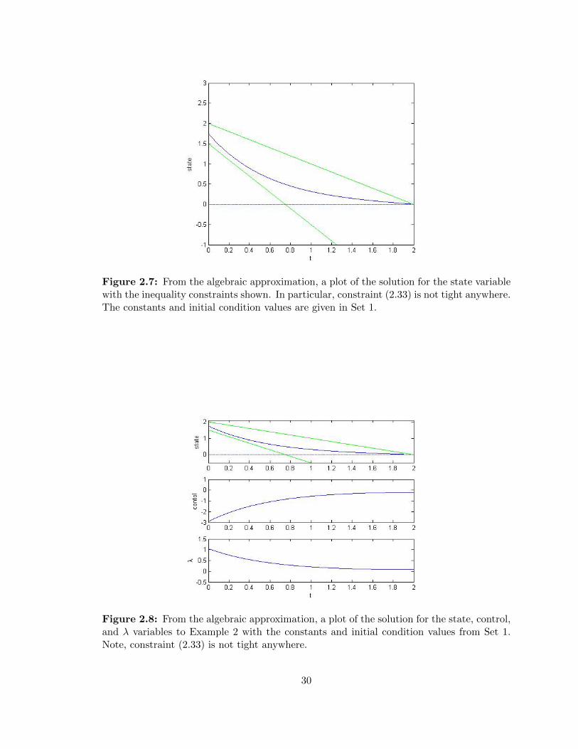
Figure 2.7: From the algebraic approximation, a plot of the solution for the state variablewith the inequality constraints shown. In particular, constraint (2.33) is not tight anywhere.The constants and initial condition values are given in Set 1.

Figure 2.8: From the algebraic approximation, a plot of the solution for the state, control,and λ variables to Example 2 with the constants and initial condition values from Set 1.Note, constraint (2.33) is not tight anywhere.

30

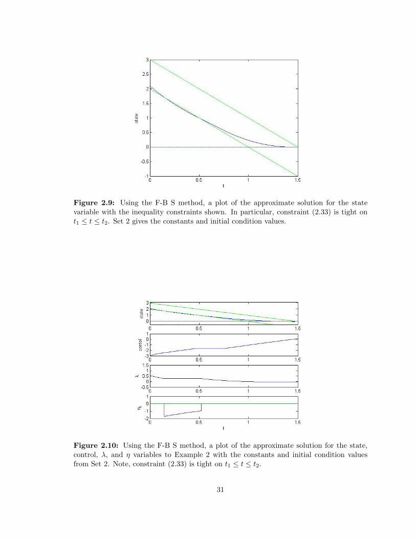
Figure 2.9: Using the F-B S method, a plot of the approximate solution for the statevariable with the inequality constraints shown. In particular, constraint (2.33) is tight ont1 ≤ t ≤ t2. Set 2 gives the constants and initial condition values.

Figure 2.10: Using the F-B S method, a plot of the approximate solution for the state,control, λ, and η variables to Example 2 with the constants and initial condition valuesfrom Set 2. Note, constraint (2.33) is tight on t1 ≤ t ≤ t2.

31

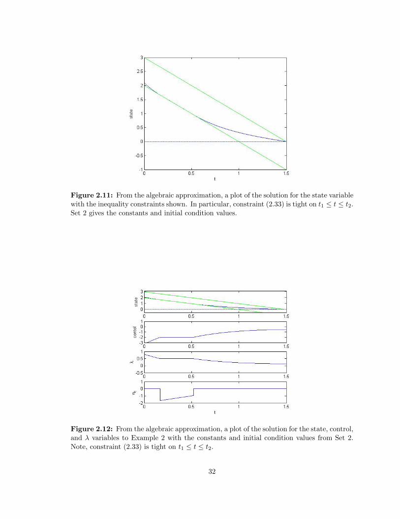
Figure 2.11: From the algebraic approximation, a plot of the solution for the state variablewith the inequality constraints shown. In particular, constraint (2.33) is tight on t1 ≤ t ≤ t2.Set 2 gives the constants and initial condition values.

Figure 2.12: From the algebraic approximation, a plot of the solution for the state, control,and λ variables to Example 2 with the constants and initial condition values from Set 2.Note, constraint (2.33) is tight on t1 ≤ t ≤ t2.

32

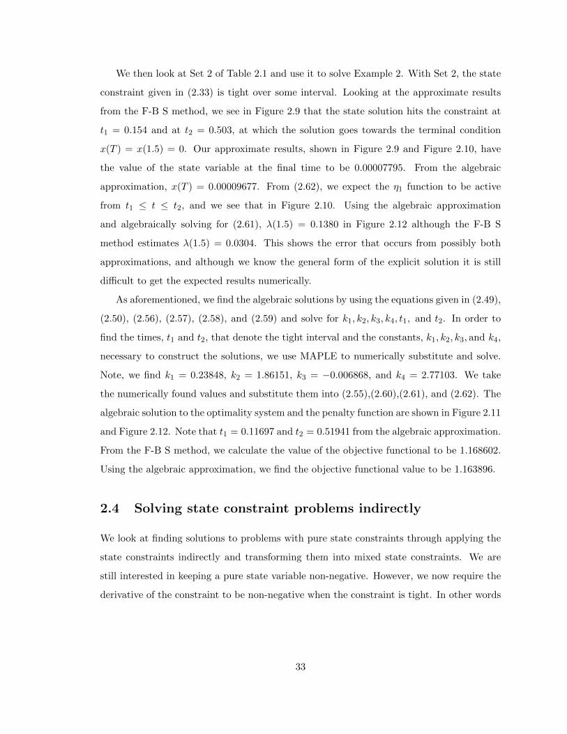
We then look at Set 2 of Table 2.1 and use it to solve Example 2. With Set 2, the state

constraint given in (2.33) is tight over some interval. Looking at the approximate results

from the F-B S method, we see in Figure 2.9 that the state solution hits the constraint at

t1 = 0.154 and at t2 = 0.503, at which the solution goes towards the terminal condition

x(T ) = x(1.5) = 0. Our approximate results, shown in Figure 2.9 and Figure 2.10, have

the value of the state variable at the final time to be 0.00007795. From the algebraic

approximation, x(T ) = 0.00009677. From (2.62), we expect the η1 function to be active

from t1 ≤ t ≤ t2, and we see that in Figure 2.10. Using the algebraic approximation

and algebraically solving for (2.61), λ(1.5) = 0.1380 in Figure 2.12 although the F-B S

method estimates λ(1.5) = 0.0304. This shows the error that occurs from possibly both

approximations, and although we know the general form of the explicit solution it is still

difficult to get the expected results numerically.

As aforementioned, we find the algebraic solutions by using the equations given in (2.49),

(2.50), (2.56), (2.57), (2.58), and (2.59) and solve for k1, k2, k3, k4, t1, and t2. In order to

find the times, t1 and t2, that denote the tight interval and the constants, k1, k2, k3, and k4,

necessary to construct the solutions, we use MAPLE to numerically substitute and solve.

Note, we find k1 = 0.23848, k2 = 1.86151, k3 = −0.006868, and k4 = 2.77103. We take

the numerically found values and substitute them into (2.55),(2.60),(2.61), and (2.62). The

algebraic solution to the optimality system and the penalty function are shown in Figure 2.11

and Figure 2.12. Note that t1 = 0.11697 and t2 = 0.51941 from the algebraic approximation.

From the F-B S method, we calculate the value of the objective functional to be 1.168602.

Using the algebraic approximation, we find the objective functional value to be 1.163896.

2.4 Solving state constraint problems indirectly

We look at finding solutions to problems with pure state constraints through applying the

state constraints indirectly and transforming them into mixed state constraints. We are

still interested in keeping a pure state variable non-negative. However, we now require the

derivative of the constraint to be non-negative when the constraint is tight. In other words

33

we require,

h1(t, x, u) ≥ 0, whenever h(t, x) = 0. (2.63)

This means we have a mixed constraint, but only when the constraint is tight. So, as

we mention in Section 2.1, the indirect method appends to the Hamiltonian a penalty

multiplier that multiplies the first time derivative of the constraint, ηh1. We define the

penalty multiplier, η(t) ≥ 0, to satisfy η ≡ 0 when the constraint is not tight, and η ≥ 0

otherwise when the constraint is tight. Note η must also satisfy the property of η′ ≤ 0.

Since we are dealing with state constraints, we must also ensure the transversality condition

and jump conditions for the adjoint equation hold[16].

Solving a state constraint problem indirectly follows the similar process as mentioned in

the direct constraint examples discussed earlier in this chapter. So we illustrate an example

of an indirect state constraint problem below with analytical results first and then our

numerical approximations.

Solve

maxu

∫ 2

0−xdt, (2.64)

subject to

x′(t) = u(t) (2.65)

with the initial condition of x(0) = 1. The control is bounded, −1 ≤ u ≤ 1. Also, we have

the inequality state constraint, h(t, x), that we define as

x(t) ≥ 0. (2.66)

We define the penalty multiplier function to be η ≥ 0 such that ηh1 = 0 for 0 ≤ t ≤ 2.

Thus η ≡ 0 when the constraint is not tight, i.e. x > 0, and η ≥ 0 when the constraint is

tight. Here h1 = u, and h1 = u ≥ 0 when h = 0.

34

Using the PMP, we first look at the Hamiltonian when the constraint is not tight, i.e.

x > 0, is

H = −x+ λu. (2.67)

Consider the derivative of the Hamiltonian with respect to the control,

∂H

∂u= λ. (2.68)

In finding the optimality condition, we investigate whether the control is bang-bang or

singular because the problem has a linear dependence on the control. The switching function

is ψ = λ and we determine the control through the methods described in Section 1.3,

u∗(t) =

umin = −1, if λ < 0

∈ [umin, umax], if λ = 0

umax = 1, if λ > 0.

(2.69)

We find the adjoint DE to be

λ′ = −∂H∂x

= 1 (2.70)

We investigate the possibility of a singular control on a subinterval by looking at the adjoint

DE when ψ = 0. From (2.69), λ = 0⇒ λ′ = 0 and this contradicts (2.70), λ′ = 1. Thus no

singular subinterval exists and the control is bang-bang over the interval, when x > 0.

However when looking at the problem while the state constraint is tight, i.e. x = 0, we

must apply the indirect maximum principle, from [16]. We find the Hamiltonian is

H = −x+ λu+ ηh1 (2.71)

= −x+ λu+ ηx′ (2.72)

= −x+ λu+ ηu. (2.73)

35

Thus the derivative of the Hamiltonian with respect to the control is

∂H

∂u= λ+ η. (2.74)

We find the switching function to be ψ = λ+ η and so the control is divided into cases. In

particular,

u∗(t) =

umin = 0, if λ+ η < 0

∈ [umin, umax], if λ+ η = 0

umax = 1, if λ+ η > 0,

(2.75)

since x′ = u ≥ 0, from h1 ≥ 0, to satisfy the state constraint in (2.66). On a subinterval

with x = 0, we have u = 0, and thus u∗ is bang-bang.

We know from the initial condition, x(0) = 1, that the constraint is not tight on an initial

subinterval, i.e. η = 0. Also, since the problem is of maximizing the objective functional,

the optimal control will be at a minimum during this subinterval, i.e. u∗ = −1 from (2.69).

Substituting this into the state DE in (2.65) yields x′ = −1. Solving for the state equation,

we use the initial condition and find that x∗ = 1 − t on some subinterval. Looking at the

state equation, it appears the state constraint in (2.66) will become tight at t = 1. Hence,

on the initial subinterval 0 ≤ t ≤ 1, the solutions of the optimal state, optimal control, and

penalty function are

x∗ = 1− t, (2.76)

u∗ = −1, (2.77)

η = 0. (2.78)

In order to determine the adjoint equation, we look at the transversality condition.

The transversality condition for the indirect method must satisfy, λ(2−) = γ ≥ 0, γx(2) =

λ(2−)x(2) = 0, from [16]. As a simple guess we try λ(2−) = γ = 0, which works since

x(2) = 0. Thus combining this guess for λ(2−) with adjoint DE (2.70), we see the solution

36

is

λ = t− 2 (2.79)

on a terminal subinterval. We know λ ≤ 0 on this subinterval. In order to decide which

control value to choose we determine if the state constraint is tight or not. However, earlier

we found that at t = 1 the state constraint becomes tight. So the optimal control on the

terminal subinterval, 1 ≤ t ≤ 2 is u∗ = 0 as defined in (2.75). Substituting this into the

state DE in (2.65) implies x∗ = c, where c is a constant. But at t = 1, we know x(1) = 0.

So, c = 0 implies x∗ = 0 for 1 ≤ t ≤ 2. Also, the constraint being tight implies from (2.75)

that η = −λ so η = 2− t ≥ 0. The terminal subinterval is 1 ≤ t ≤ 2 on which the solutions

to the optimality system and penalty function are

x∗ = 0, (2.80)

u∗ = 0, (2.81)

λ = t− 2, (2.82)

η = 2− t. (2.83)

We seek the adjoint equation on the initial subinterval, 0 ≤ t ≤ 1, by examining what

happens at the jump τ = 1. From λ = t− 2, at τ = 1, λ(1+) = −1. For λ(1−), we look at

H(1+) and H(1−). In particular, applying (2.4),

H(1+) = −x∗(1+) + λ(1+)u∗(1+) = 0 (2.84)

H(1−) = −x∗(1−) + λ(1−)u∗(1−) (2.85)

must be equal. Using x∗(1+) = x∗(1−) = 0, u∗(1+) = 0, and u∗(1−) = −1, we have

λ(1−) = 0. So solving (2.70) with λ(1−) = 0 implies λ = t− 1 for 0 ≤ t ≤ 1. The value of

the jump, determined from (2.3), is ζ(1) = λ(1−)− λ(1+) = 1 ≥ 0.

37

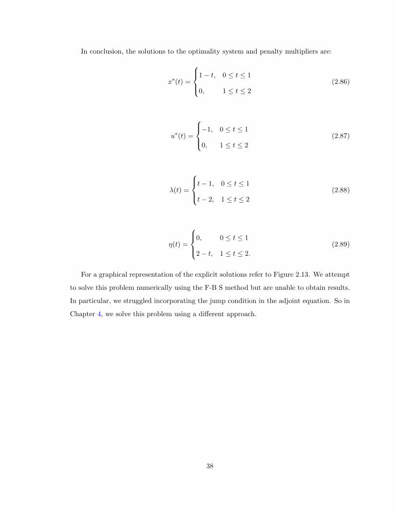
In conclusion, the solutions to the optimality system and penalty multipliers are:

x∗(t) =

1− t, 0 ≤ t ≤ 1

0, 1 ≤ t ≤ 2

(2.86)

u∗(t) =

−1, 0 ≤ t ≤ 1

0, 1 ≤ t ≤ 2

(2.87)

λ(t) =

t− 1, 0 ≤ t ≤ 1

t− 2, 1 ≤ t ≤ 2

(2.88)

η(t) =

0, 0 ≤ t ≤ 1

2− t, 1 ≤ t ≤ 2.

(2.89)

For a graphical representation of the explicit solutions refer to Figure 2.13. We attempt

to solve this problem numerically using the F-B S method but are unable to obtain results.

In particular, we struggled incorporating the jump condition in the adjoint equation. So in

Chapter 4, we solve this problem using a different approach.

38

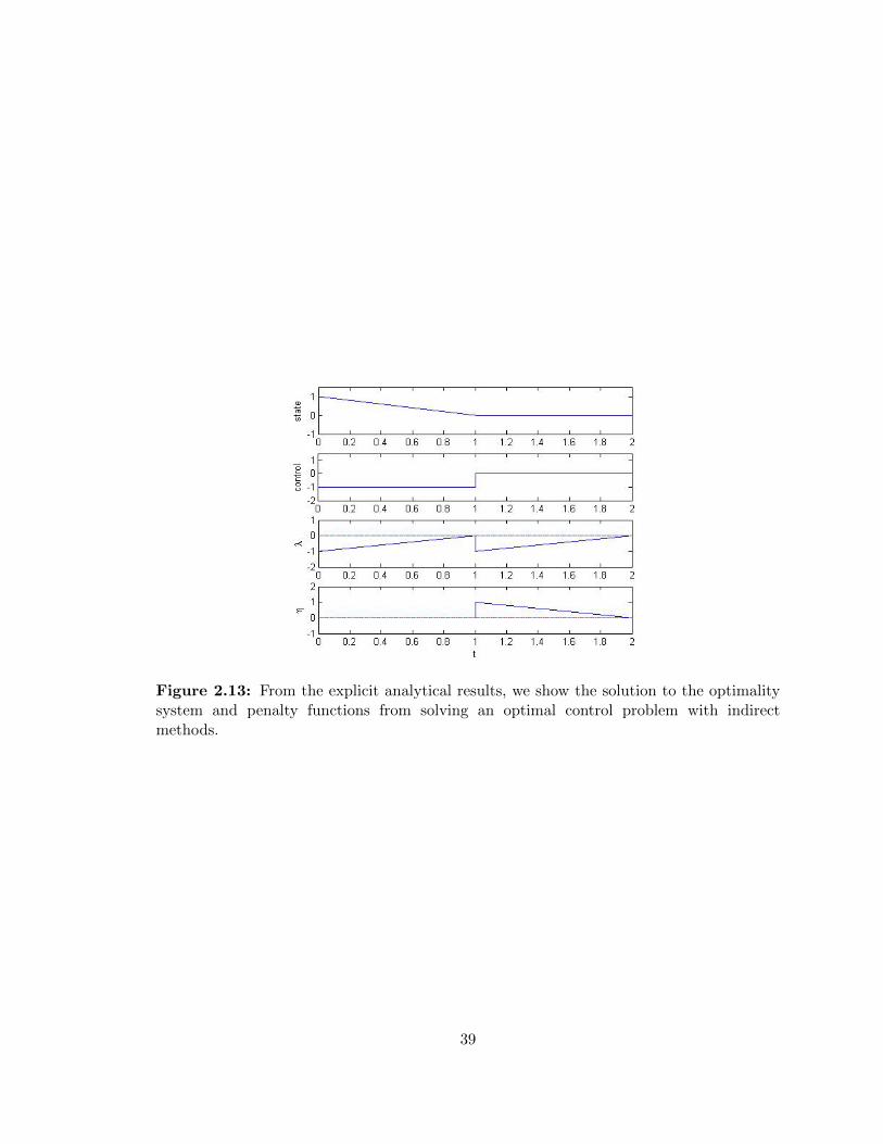
Figure 2.13: From the explicit analytical results, we show the solution to the optimalitysystem and penalty functions from solving an optimal control problem with indirectmethods.

39

Chapter 3

Runner Problem

3.1 Introduction

Running is an easily accessible and highly competitive sport. The origins of human running

is thought to have evolved at least four and a half million years ago, primarily out of the

necessity to hunt and survive. Competitive running as a display of endurance dates back

to the Olympics in 776 B.C. Running is an activity for people of all ages, shapes, and sizes

and is growing in popularity. With so many people participating in this sport, we wanted

to try and find a way for people to run their best. In other words, we want to identify the

ideal strategy for a runner competing in a race.

In order to solve this running problem we must transform this real world problem to

have a more quantitative form. In other words, we need to create a mathematical model

that represents a runner running a race. If the goal is to minimize time for running a

specific distance, or similarly to maximize the running distance for a specific time, then the

runner’s speed, or velocity, will mainly determine this system. Simply put, how long it takes

to run a race depends on the velocity of the runner. The velocity of a runner is determined

by many factors: physiological, mental, and environmental. A more complete model could

include mental focus, wind, humidity, temperature, terrain, energy levels, drafting, energy

replenishment, and biomechanics. However, in our attempt to model this optimal running

strategy, only some of the physiological factors will be addressed. Previous work has been

done to determine the optimal strategy for a competitor running a race. In particular,

40

Keller concluded a runner’s velocity depends on: the maximum force he or she can exert,

the resistive force opposing the runner, the rate at which oxygen metabolism supplies energy,

and the initial amount of energy stored in the runner [7]. We will use Keller’s model as a

basis for ours.

Keller’s problem seeks how best to control the runner’s force to run the farthest distance

in a given time. Force is under the runner’s control and directly impacts velocity. He

determined the physiological parameters, that velocity depends on, from world records using

least-squares fitting. He then solved the maximization problem using Newton’s Second Law

and calculus of variations. Keller found that for all races less than 291 meters, the runner

should run at maximum acceleration. Races greater than 291 meters identify the strategy

of attaining maximum acceleration early, then maintaining a constant speed throughout

the race until the final seconds when slowing down occurs and energy should be nearly

exhausted. Essentially there are three subarcs: a starting phase, a constant interval, and a

finishing phase. The first two subarcs are controlled by initial energy amounts and energy

provided from breathing and circulation, and the last subarc is determined just from energy

gained by breathing and circulation [7].

However, in the real world, is is noteworthy to mention that races often finish with a kick

as opposed to the negative kick suggested in his optimal solution. Keller states the difference

either being the runners are not running optimally or that the theory is inaccurate. Winning

is often more important than minimizing time, thus affecting strategy. Keller suggests that

if runners ran at their optimal speed determined by the theory, then they might win by

even more [7].

Keller’s model has previously been extended and modified to become more realistic. In

particular, Woodside added a fatigue term for longer distance races. For modeling races

longer than 10,000 meters, the fatigue term reduces the runner’s energy and is cumulative

over time, which makes sense because although breathing and circulation replenish energy

it should become less effective the longer one runs [18]. Behncke published detailed papers

that included three submodels based on the biomechanics, energetics, and the typical

optimization model. More specifically, he looked at the processes of chemical energy being

converted to mechanical energy [1]. Quinn included starting gun reaction time, which plays

more of a role in sprint races, and included cross winds and running on a curved track

41

with maximum force diminishing slowly over time. Pitcher built a coupled two-runner

model that included air resistance and drafting. By assigning one runner to run according

to Keller’s optimal strategy, Pitcher was able to show how various initial conditions and

drafting affected the strategy of the other runner [14].

3.2 Background

Our problem, like Keller’s, is how to optimally control the runner’s force to run the farthest

distance in a given time. Force is under the runner’s control and directly impacts velocity.

Based on Newton’s Second Law, the equation of motion is

Mv′(t) = Ft −Rint(v, x, t)−Rext(v, x, t) (3.1)

where v′(t) is the derivative of velocity, also known as acceleration, M is the mass of the

runner, Ft is the propelling force generated from the legs, Rint,Rext are the resistive internal

and external forces, and x(t) is the position of the runner. We assume the race takes place

on a smooth flat track (one dimension), environmental factors are a non-issue, and there

are no physical or mental differences among runners [1]. So we drop the dependency of Rint

and Rext on x. From Behncke’s model, oxygen consumption is an internal resistive force

we acknowledge and we assume it is proportional to velocity [1]. The previous assumptions

allows us to reduce (3.1) to be

v′(t) = f(t)−Rint(v, t) (3.2)

where f(t) is the force per unit mass and Rint loses the x variable because of the homogeneity

of the track. This force per unit mass is bounded above, meaning there is a maximum

amount of force a runner can exert. Consequently, this equation of motion is the basis for

the first state differential equation of our model.

The amount of energy a runner has also limits his velocity. The runner has an initial

amount of energy, E0. As one runs, energy decreases based on the amount of work he or

she is doing and is replenished through breathing and circulation. From physics, we know

work equals force times distance and thus the integration of a rate of change, velocity, gives

42

distance. Breathing and circulation supply oxygen throughout the body so that the muscles

can consume more energy. So the rate of change in energy can be thought of as

E′(t) = b− f(t)v(t) (3.3)

where v(t) is velocity and b is the rate at which oxygen is supplied per unit mass in excess of

the non-running metabolism by breathing and circulation. Consequently, this equation of

energy flow is the basis for the second state differential equation of our model. For physical

reasonableness, the amount of energy can not be negative. Thus we have an an inequality

state constraint which must be considered. Ideally, the runner should finish the race with

as little energy as possible. This means one should put forth all the effort he or she can to

maximize their distance.

Keller solved this problem using calculus of variations, and Pitcher and Behncke used

optimal control theory. We will also use optimal control theory as it is a suitable method

for optimizing a function subject to some state equations and constraints [1],[14]. Pitcher

recreated Keller’s work for a track race of 800m, thus we will do the same to ensure our

methods are correct. However, the theory developed by Keller is suitable for a race of

any length, as Keller predicted results for races as short as 50 yards up to 10,000 meters.

However, Woodside amended the model to be more accurate for races over 10,000 meters

up to 275,000 meters [18].

3.3 Mathematical Model

Restating our problem, we want to maximize the distance a runner can cover in a given

time by controlling the runner’s force. Force is under the runner’s control, so it will be our

control variable given by u(t), and it directly impacts velocity. Bounds for the propulsive

force are

0 ≤ u(t) ≤ F. (3.4)

Velocity is essentially the runner’s pace or speed, thus we want to maximize this, as

efficiently as possible, during the race to maximize the distance. Let x1(t) be velocity,

43

then based off the equation of motion in (2), the acceleration, or rate of change in velocity,

of the runner is given by

x′1(t) = u(t)− x1(t)

a. (3.5)

Thus the internal resistive force per unit mass is proportional to velocity, by a constant of

1/a. At the start of the race, the runner is not moving, so

x1(0) = 0 (3.6)

is an initial condition.

The amount of energy a runner has, x2(t) at time t, also limits the runner’s force. Let

x2(t) be the energy equivalent of the available oxygen per unit mass. The initial energy

amount, x2(0), is denoted by x20 . Also, for the model to make sense physically,

x2(t) ≥ 0 (3.7)

must be satisfied, i.e. energy must be non-negative. This is an inequality state constraint

that provides challenging and interesting results, as discussed in Section 2. Ideally for a

runner to run the fastest race he or she can, he or she should finish the race with as minimal

energy as possible, but it cannot be negative.

The rate of change of energy, x′2, increases by a constant breathing and circulation rate,

b, and decreases by the propulsive force times velocity, u(t)v(t), also known as work of the

runner, similar to (3.3), so we have

x′2(t) = b− x1(t)u(t). (3.8)

We set up our problem to be solved using optimal control theory. Thus x1(t) and x2(t)

are the state variables and u(t) is the control. Previous work set up the optimal control

problem to have a linear dependence on the control. The optimal solution consists of three

subarcs: a starting interval, a singular interval, and a finishing interval. While searching

for the optimal solution, obtaining the large singular interval may be difficult. So we also

44

formulate the optimal control problem to have quadratic dependence on the control. We

know a small quadratic dependence on the control can approximate the linear dependence

formulation well.

First we look at the optimal control problem with the control occurring in a linear way

in the Hamiltonian. The objective functional to be maximized is given by

J(u) =

∫ T

0x1(t)dt, (3.9)

and is subject to (3.4),(3.5),(3.6),(3.7), and (3.8).We seek to maximize J(u) over the

set U = {u : [0, T ]→ R|u piecewise continuous }. Notice the u(t) occurs linearly in the

state equations. Thus in solving for the optimality system we investigate the presence

of the singular subarcs and compare the results when including or disregarding the energy

constraint, (3.7). The analytical and numerical results and discussion of the optimal control

problem with linear dependence on the control is explained in Section 3.4.

Then second we approximate our problem by constructing an optimal control problem

with the control occurring in a quadratic way in the Hamiltonian. The objective functional

is given by

J(u) =

∫ T

0(x1(t)− εu2(t))dt (3.10)

and is subject to (3.4),(3.5),(3.6),(3.7),(3.8), and ε being small with 0 < ε ≤ 1. We seek to

maximize J(u) over the set U = {u : [0, T ]→ R|u piecewise continuous }. Thus in solving

for the optimality system we compare the results when including or disregarding the energy

constraint, (3.7). The analytical and numerical results and discussion of the optimal control

problem with quadratic dependence on the control is explained in Section 3.5.

For values of the parameters used in solving the optimal control problem with linear or

quadratic dependence on the control, refer to Table 3.1. Note, like Pitcher, we try to find

the optimality systems for the optimal control problems by having the given final time be

1:41.11. By setting T = 101.11 sec, this denotes the men’s 800m world record time in 2009.

We can choose any reasonable length of time and similar results should occur. Since we

wanted to replicate Pitcher’s results we focused on T = 101.11 sec.

45

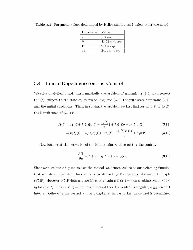
Table 3.1: Parameter values determined by Keller and are used unless otherwise noted.

Parameter Value

a 1.0 sec

b 41.56 m2/sec2

F 9.9 N/kg

x20 2409 m2/sec2

3.4 Linear Dependence on the Control

We solve analytically and then numerically the problem of maximizing (3.9) with respect

to u(t), subject to the state equations of (3.5) and (3.8), the pure state constraint (3.7),

and the initial conditions. Thus, in solving the problem we first find for all u(t) in [0, T ],

the Hamiltonian of (3.9) is

H(t) = x1(t) + λ1(t)(u(t)− x1(t)

a

)+ λ2(t)(b− x1(t)u(t)) (3.11)

= u(λ1(t)− λ2(t)x1(t)) + x1(t)−λ1(t)x1(t)

a+ λ2(t)b. (3.12)

Now looking at the derivative of the Hamiltonian with respect to the control,

∂H

∂u= λ1(t)− λ2(t)x1(t) = ψ(t). (3.13)

Since we have linear dependence on the control, we denote ψ(t) to be our switching function

that will determine what the control is as defined by Pontryagin’s Maximum Principle

(PMP). However, PMP does not specify control values if ψ(t) = 0 on a subinterval t1 ≤ t ≤

t2 for t1 < t2. Thus if ψ(t) = 0 on a subinterval then the control is singular, using, on that

interval. Otherwise the control will be bang-bang. In particular the control is determined

46

by,

u∗(t) =

0, if ψ(t) < 0

using(t), if ψ(t) = 0

F, if ψ(t) > 0,

(3.14)

where F comes from the bounds on u(t) in (3.4).

For simplicity and for general understanding of the problem, we solve the problem

without the energy state constraint given in (3.7). From PMP, the the adjoint differential

equations are:

λ′1(t) = −∂H∂x1

=λ1(t)

a+ λ2(t)u(t)− 1 (3.15)

λ′2(t) = −∂H∂x2

= 0 (3.16)

with transversality conditions λ1(T ) = 0 and λ2(T ) = 0.

For brevity, the explicit dependence of the state variable on t is often suppressed.

Thinking about the problem qualitatively, we expect the runner’s force to be maximal,

without any regard to energy depletion, in order to run the farthest distance. From (3.17)

and the transversality condition λ2(T ) = 0, we know that λ2 ≡ 0. Thus, ψ = λ1 implies

(3.15) becomes λ′1 =λ1a− 1. From the transversality condition of λ1(T ) = 0 and the

structure of the λ1 DE, we know λ1(t) ≥ 0. However, ψ = λ1 = 0 implies that λ′1 = 0. So,

0 =λ1a− 1 is a contradiction. So the control is bang-bang, and as we expect, the runner’s

force should be maximal for the entire run. This system was implemented numerically using

techniques described in Section 1.5, and the results can be seen in Figure 3.1. We note that

energy, x2, becomes negative.

47

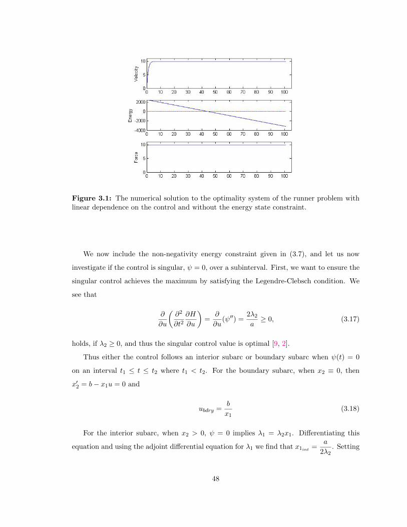
Figure 3.1: The numerical solution to the optimality system of the runner problem withlinear dependence on the control and without the energy state constraint.

We now include the non-negativity energy constraint given in (3.7), and let us now

investigate if the control is singular, ψ = 0, over a subinterval. First, we want to ensure the

singular control achieves the maximum by satisfying the Legendre-Clebsch condition. We

see that

∂

∂u

(∂2

∂t2∂H

∂u

)=

∂

∂u(ψ′′) =

2λ2a≥ 0, (3.17)

holds, if λ2 ≥ 0, and thus the singular control value is optimal [9, 2].

Thus either the control follows an interior subarc or boundary subarc when ψ(t) = 0

on an interval t1 ≤ t ≤ t2 where t1 < t2. For the boundary subarc, when x2 ≡ 0, then

x′2 = b− x1u = 0 and

ubdry =b

x1(3.18)

For the interior subarc, when x2 > 0, ψ = 0 implies λ1 = λ2x1. Differentiating this

equation and using the adjoint differential equation for λ1 we find that x1int =a

2λ2. Setting

48

the derivative of x1int equal to the x1 state differential equation gives

uint =x1int

a. (3.19)

However, energy can still be negative and so we attempt to fix this by appending the

term which includes the penalty function directly multiplying the pure state constraint, as

discussed in Chapter 2. What makes implementing this inequality constraint difficult is that

x2 does not show up anywhere explicitly in the system. So as Behncke and Pitcher included

in [1] and [14], we include the state constraint directly in the Hamiltonian by adjoining it

to the η, or penalty function. The penalty function is defined as, η(t) ≥ 0 and

ηx2 = 0 (3.20)

for all time, meaning η ≡ 0 when x2 > 0, and η ≥ 0 otherwise. The Hamiltonian becomes

H = u(λ1 − λ2x1) + x1 −λ1x1a

+ λ2b+ ηx2. (3.21)

The λ′1 equation is the same as (3.15), but λ′2 = −∂H∂x2

= −η. Since x2 = 0 this implies

x′2 = 0. Also, ψ(t) = 0⇒ λ1 = λ2x1. Using these equations, along with the state DEs, we

find

η =1

x1

[1− 2λ1

a

]. (3.22)

As Keller described, we anticipate three subarcs: a brief starting phase, a long constant

interval, and a short finishing phase. Essentially, the control wants to remain in the singular

case over the entire interval except for at the start when force should be maximal and then

at the finish when force should be minimal.

Getting these expected results is difficult. This system was implemented numerically

using F-B S, described in Section 1.5, and the results can be seen in Figures 3.2-3.5. The

step size for approximating the DEs is ∆t = .0101. For convergence, the relative error for

values of successive iterations needs to be less than the tolerance of 10−4. We find that the

system is very sensitive to the method of updating the control. When solving the runner

49

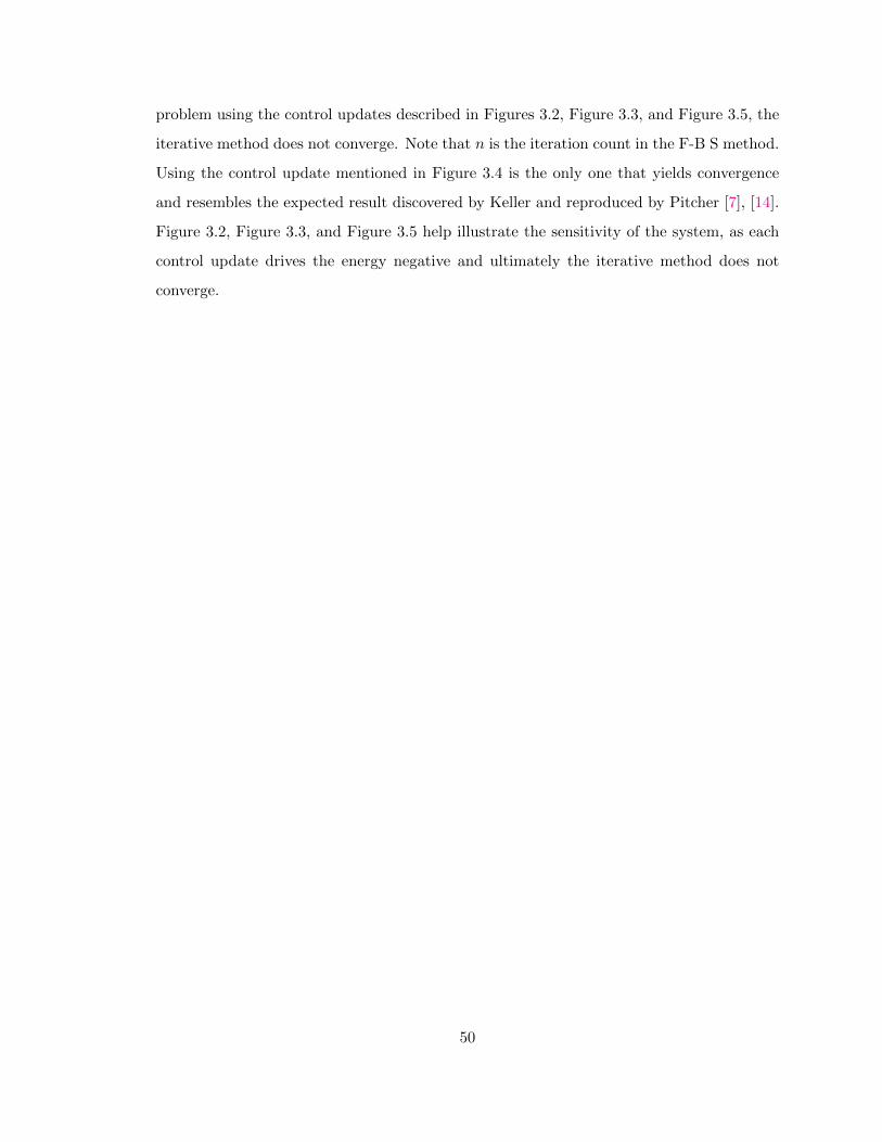
problem using the control updates described in Figures 3.2, Figure 3.3, and Figure 3.5, the

iterative method does not converge. Note that n is the iteration count in the F-B S method.

Using the control update mentioned in Figure 3.4 is the only one that yields convergence

and resembles the expected result discovered by Keller and reproduced by Pitcher [7], [14].

Figure 3.2, Figure 3.3, and Figure 3.5 help illustrate the sensitivity of the system, as each

control update drives the energy negative and ultimately the iterative method does not

converge.

50

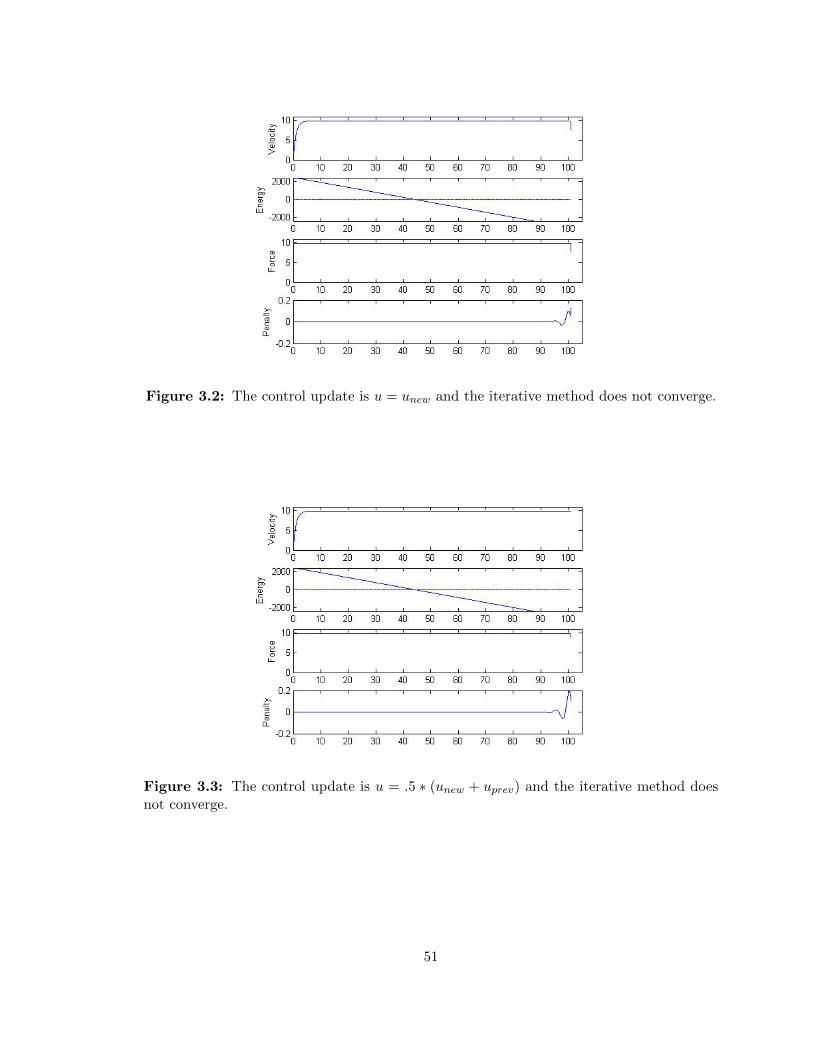
Figure 3.2: The control update is u = unew and the iterative method does not converge.

Figure 3.3: The control update is u = .5 ∗ (unew + uprev) and the iterative method doesnot converge.

51

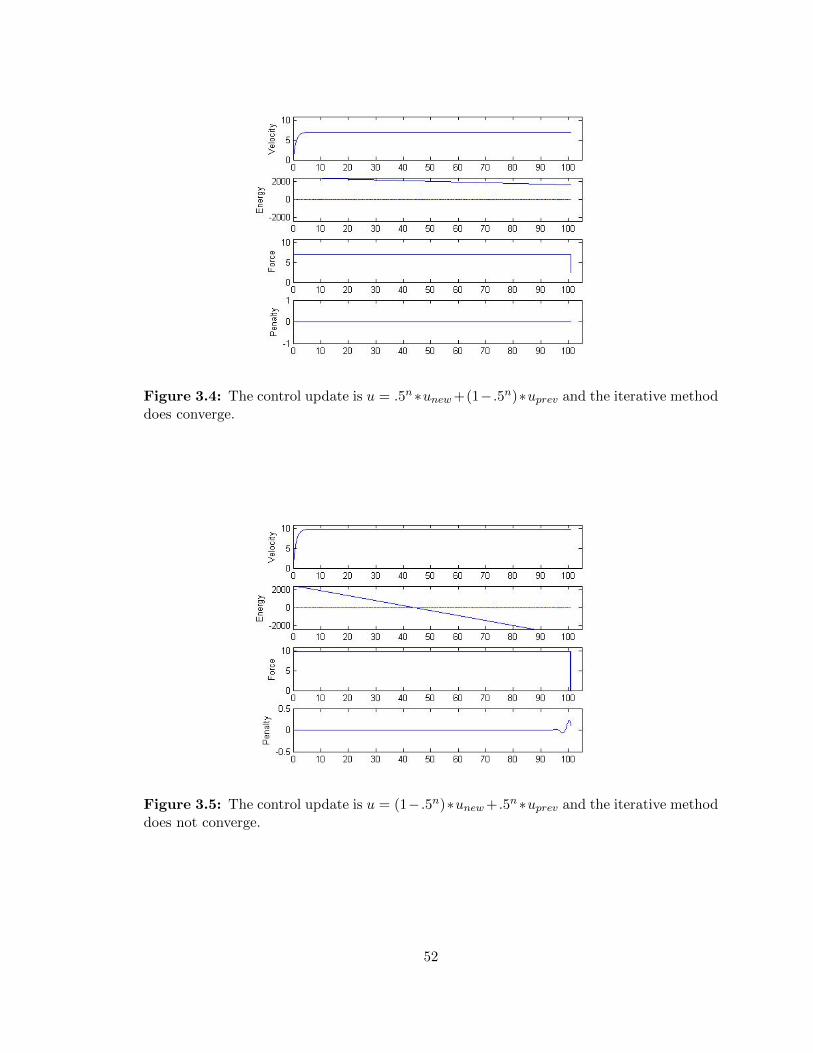
Figure 3.4: The control update is u = .5n∗unew+(1− .5n)∗uprev and the iterative methoddoes converge.

Figure 3.5: The control update is u = (1− .5n)∗unew+ .5n∗uprev and the iterative methoddoes not converge.

52

We acknowledge the difficulty of solving this problem and note that Pitcher had better

success. Referring to Pitcher’s work in [14] and [13], we see that explicitly deriving a

solution structure of two junction times and algebraically solving for the resulting systems of

equations yields better results. This problem is unique because the control wants to remain

in the singular case except for small times at the beginning and end of the race. So we

reformulate the problem slightly to avoid the singularity by having a quadratic dependence

on the control.

3.5 Quadratic Dependence on the Control

We solve analytically and then numerically the problem of maximizing (3.10) with respect

to u(t), subject to the state equations of (3.5) and (3.8), the pure state constraint (3.7),

and the initial conditions. Thus, in solving the problem we first find for all u(t) in [0, T ],

the Hamiltonian of (3.10) is

H = x1 − εu2 + λ1(u− x1

a

)+ λ2(b− x1u). (3.23)

The derivative of the Hamiltonian with respect to the control is

∂H

∂u=λ1 − λ2x1

2ε. (3.24)

We ensure this is a maximization problem by finding the second derivative of the

Hamiltonian with respect to the control,

∂2H

∂u2= −2ε ≤ 0, (3.25)

and note that the inequality holds for all ε > 0.

From PMP, the the adjoint differential equations are:

λ′1 = −∂H∂x1

=λ1a

+ λ2u− 1 (3.26)

53

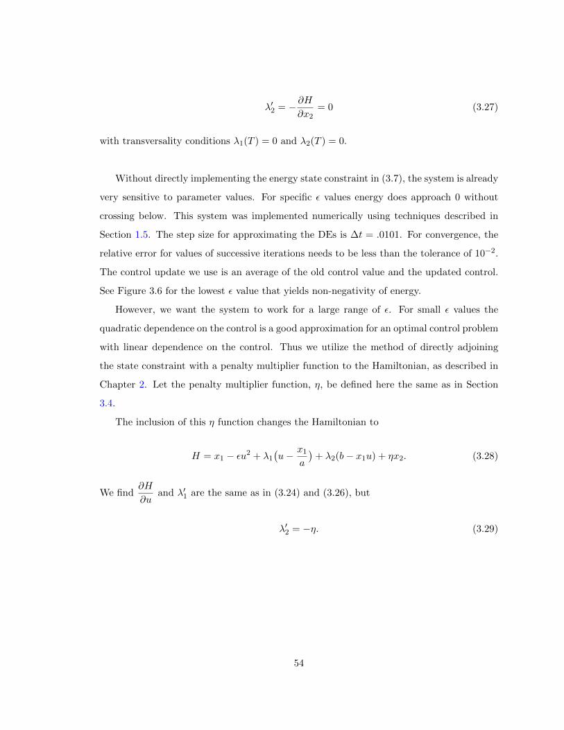
λ′2 = −∂H∂x2

= 0 (3.27)

with transversality conditions λ1(T ) = 0 and λ2(T ) = 0.

Without directly implementing the energy state constraint in (3.7), the system is already

very sensitive to parameter values. For specific ε values energy does approach 0 without

crossing below. This system was implemented numerically using techniques described in

Section 1.5. The step size for approximating the DEs is ∆t = .0101. For convergence, the

relative error for values of successive iterations needs to be less than the tolerance of 10−2.

The control update we use is an average of the old control value and the updated control.

See Figure 3.6 for the lowest ε value that yields non-negativity of energy.

However, we want the system to work for a large range of ε. For small ε values the

quadratic dependence on the control is a good approximation for an optimal control problem

with linear dependence on the control. Thus we utilize the method of directly adjoining

the state constraint with a penalty multiplier function to the Hamiltonian, as described in

Chapter 2. Let the penalty multiplier function, η, be defined here the same as in Section

3.4.

The inclusion of this η function changes the Hamiltonian to

H = x1 − εu2 + λ1(u− x1

a

)+ λ2(b− x1u) + ηx2. (3.28)

We find∂H

∂uand λ′1 are the same as in (3.24) and (3.26), but

λ′2 = −η. (3.29)

54

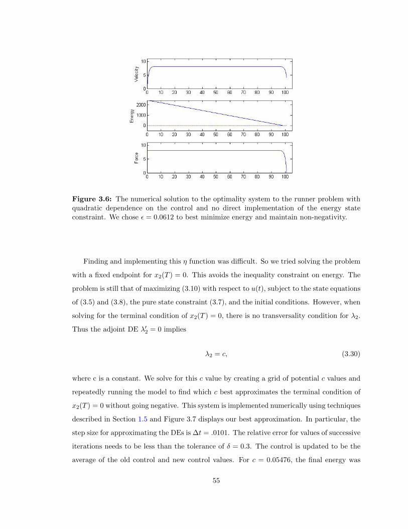
Figure 3.6: The numerical solution to the optimality system to the runner problem withquadratic dependence on the control and no direct implementation of the energy stateconstraint. We chose ε = 0.0612 to best minimize energy and maintain non-negativity.

Finding and implementing this η function was difficult. So we tried solving the problem

with a fixed endpoint for x2(T ) = 0. This avoids the inequality constraint on energy. The

problem is still that of maximizing (3.10) with respect to u(t), subject to the state equations

of (3.5) and (3.8), the pure state constraint (3.7), and the initial conditions. However, when

solving for the terminal condition of x2(T ) = 0, there is no transversality condition for λ2.

Thus the adjoint DE λ′2 = 0 implies

λ2 = c, (3.30)

where c is a constant. We solve for this c value by creating a grid of potential c values and

repeatedly running the model to find which c best approximates the terminal condition of

x2(T ) = 0 without going negative. This system is implemented numerically using techniques

described in Section 1.5 and Figure 3.7 displays our best approximation. In particular, the

step size for approximating the DEs is ∆t = .0101. The relative error for values of successive

iterations needs to be less than the tolerance of δ = 0.3. The control is updated to be the

average of the old control and new control values. For c = 0.05476, the final energy was

55

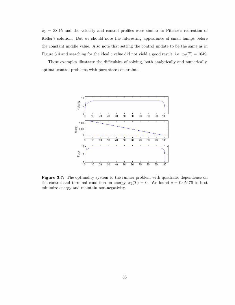
x2 = 38.15 and the velocity and control profiles were similar to Pitcher’s recreation of

Keller’s solution. But we should note the interesting appearance of small humps before

the constant middle value. Also note that setting the control update to be the same as in

Figure 3.4 and searching for the ideal c value did not yield a good result, i.e. x2(T ) = 1649.

These examples illustrate the difficulties of solving, both analytically and numerically,

optimal control problems with pure state constraints.

Figure 3.7: The optimality system to the runner problem with quadratic dependence onthe control and terminal condition on energy, x2(T ) = 0. We found c = 0.05476 to bestminimize energy and maintain non-negativity.

56

Chapter 4

Alternative Optimization

Approaches and Conclusions

4.1 GPOPS

Using a different approach to solving optimal control problems, we solve the examples

in Chapters 2, 3. We find the optimal solutions through using the General-Purpose

Pseudospectral Optimal Control Software (GPOPS) implemented in MATLAB created by

[12].

GPOPS runs an hp-adaptive Radau pseudospectral Gaussian quadrature method where

the collocation is at the Legendre-Gauss-Radau quadrature points [12]. GPOPS takes in

all the common input of an optimal control problem (objective functional, state equations,

constraints, initial and terminal conditions, and bounds) and formulates it into a non-

linear problem which is solved through the Interior Point Optimizer (IPOPT) software

implemented in MATLAB. IPOPT is a software package for solving nonlinear objectives

subject to nonlinear constraints through using primal-dual interior point methodology [17].

Further theory on the Radau pseudospectral method can be found in [5, 3, 4]. GPOPS

runs a non-linear problem solver in MATLAB, and in our examples we use IPOPT with a

tolerance of 10−7.

The conditions for setting up the refinement mesh are as follows:

57

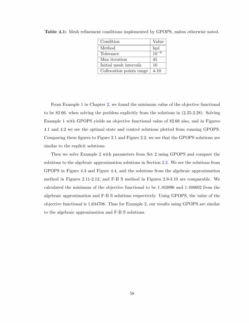
Table 4.1: Mesh refinement conditions implemented by GPOPS, unless otherwise noted.

Condition Value

Method hp1

Tolerance 10−6

Max iteration 45

Initial mesh intervals 10

Collocation points range 4-10

From Example 1 in Chapter 2, we found the minimum value of the objective functional

to be 82.66. when solving the problem explicitly from the solutions in (2.25-2.28). Solving

Example 1 with GPOPS yields an objective functional value of 82.66 also, and in Figures

4.1 and 4.2 we see the optimal state and control solutions plotted from running GPOPS.

Comparing these figures to Figure 2.1 and Figure 2.2, we see that the GPOPS solutions are

similar to the explicit solutions.

Then we solve Example 2 with parameters from Set 2 using GPOPS and compare the

solutions to the algebraic approximation solutions in Section 2.3. We see the solutions from

GPOPS in Figure 4.3 and Figure 4.4, and the solutions from the algebraic approximation

method in Figures 2.11-2.12, and F-B S method in Figures 2.9-3.10 are comparable. We

calculated the minimum of the objective functional to be 1.163896 and 1.168602 from the

algebraic approximation and F-B S solutions respectively. Using GPOPS, the value of the

objective functional is 1.634708. Thus for Example 2, our results using GPOPS are similar

to the algebraic approximation and F-B S solutions.

58

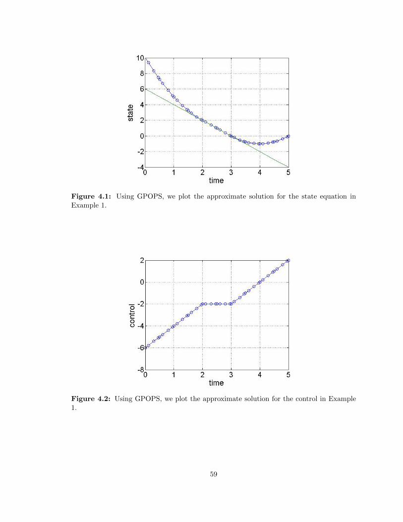
Figure 4.1: Using GPOPS, we plot the approximate solution for the state equation inExample 1.

Figure 4.2: Using GPOPS, we plot the approximate solution for the control in Example1.

59

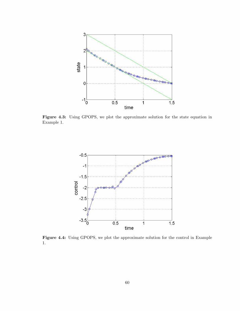
Figure 4.3: Using GPOPS, we plot the approximate solution for the state equation inExample 1.

Figure 4.4: Using GPOPS, we plot the approximate solution for the control in Example1.

60

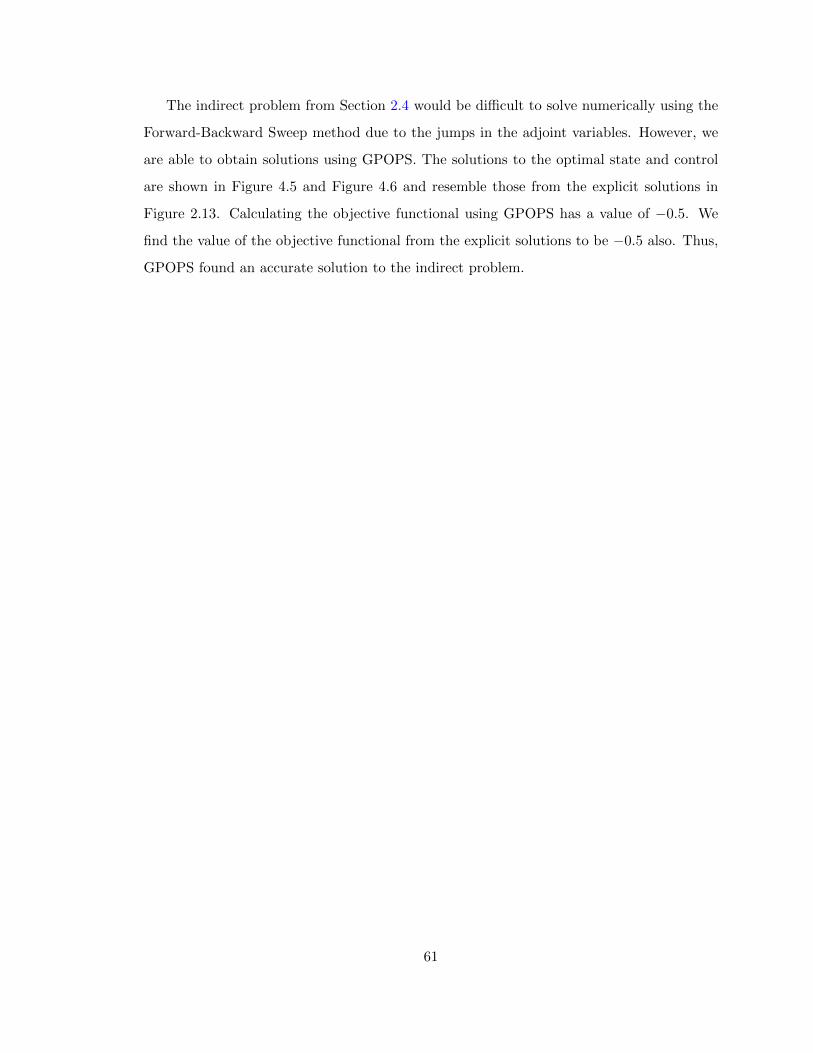
The indirect problem from Section 2.4 would be difficult to solve numerically using the

Forward-Backward Sweep method due to the jumps in the adjoint variables. However, we

are able to obtain solutions using GPOPS. The solutions to the optimal state and control

are shown in Figure 4.5 and Figure 4.6 and resemble those from the explicit solutions in

Figure 2.13. Calculating the objective functional using GPOPS has a value of −0.5. We

find the value of the objective functional from the explicit solutions to be −0.5 also. Thus,

GPOPS found an accurate solution to the indirect problem.

61

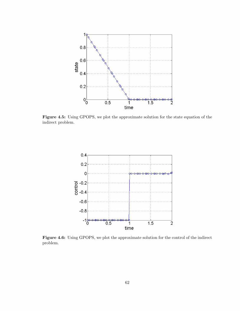
Figure 4.5: Using GPOPS, we plot the approximate solution for the state equation of theindirect problem.

Figure 4.6: Using GPOPS, we plot the approximate solution for the control of the indirectproblem.

62

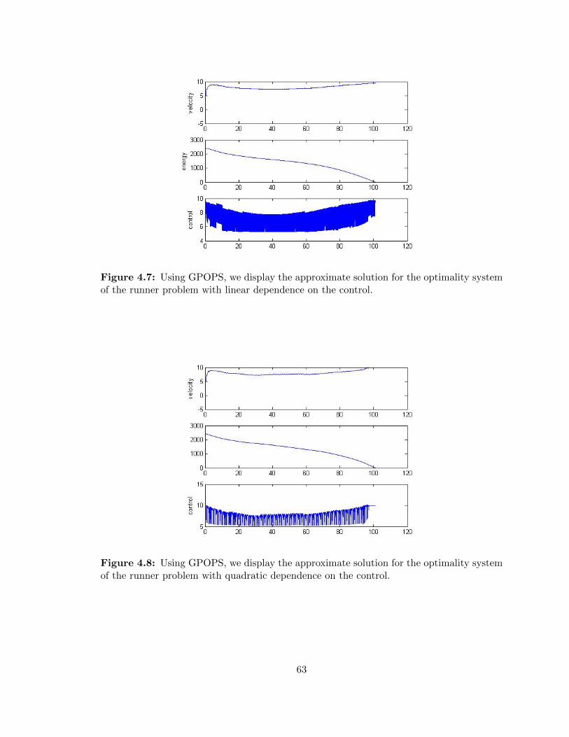
Figure 4.7: Using GPOPS, we display the approximate solution for the optimality systemof the runner problem with linear dependence on the control.

Figure 4.8: Using GPOPS, we display the approximate solution for the optimality systemof the runner problem with quadratic dependence on the control.

63

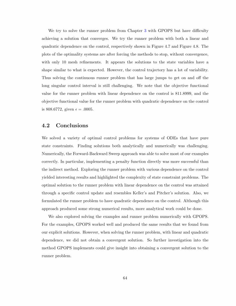
We try to solve the runner problem from Chapter 3 with GPOPS but have difficulty

achieving a solution that converges. We try the runner problem with both a linear and

quadratic dependence on the control, respectively shown in Figure 4.7 and Figure 4.8. The

plots of the optimality systems are after forcing the methods to stop, without convergence,

with only 10 mesh refinements. It appears the solutions to the state variables have a

shape similar to what is expected. However, the control trajectory has a lot of variability.

Thus solving the continuous runner problem that has large jumps to get on and off the

long singular control interval is still challenging. We note that the objective functional

value for the runner problem with linear dependence on the control is 811.8999, and the

objective functional value for the runner problem with quadratic dependence on the control

is 808.6772, given ε = .0005.

4.2 Conclusions

We solved a variety of optimal control problems for systems of ODEs that have pure

state constraints. Finding solutions both analytically and numerically was challenging.

Numerically, the Forward-Backward Sweep approach was able to solve most of our examples

correctly. In particular, implementing a penalty function directly was more successful than

the indirect method. Exploring the runner problem with various dependence on the control

yielded interesting results and highlighted the complexity of state constraint problems. The

optimal solution to the runner problem with linear dependence on the control was attained

through a specific control update and resembles Keller’s and Pitcher’s solution. Also, we

formulated the runner problem to have quadratic dependence on the control. Although this

approach produced some strong numerical results, more analytical work could be done.

We also explored solving the examples and runner problem numerically with GPOPS.

For the examples, GPOPS worked well and produced the same results that we found from

our explicit solutions. However, when solving the runner problem, with linear and quadratic

dependence, we did not obtain a convergent solution. So further investigation into the

method GPOPS implements could give insight into obtaining a convergent solution to the

runner problem.

64

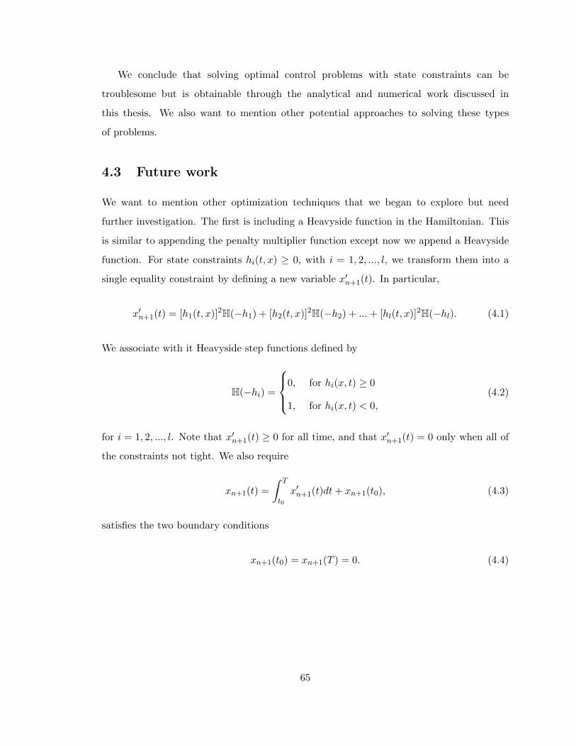
We conclude that solving optimal control problems with state constraints can be

troublesome but is obtainable through the analytical and numerical work discussed in

this thesis. We also want to mention other potential approaches to solving these types

of problems.

4.3 Future work

We want to mention other optimization techniques that we began to explore but need

further investigation. The first is including a Heavyside function in the Hamiltonian. This

is similar to appending the penalty multiplier function except now we append a Heavyside

function. For state constraints hi(t, x) ≥ 0, with i = 1, 2, ..., l, we transform them into a

single equality constraint by defining a new variable x′n+1(t). In particular,

x′n+1(t) = [h1(t, x)]2H(−h1) + [h2(t, x)]2H(−h2) + ...+ [hl(t, x)]2H(−hl). (4.1)

We associate with it Heavyside step functions defined by

H(−hi) =

0, for hi(x, t) ≥ 0

1, for hi(x, t) < 0,

(4.2)

for i = 1, 2, ..., l. Note that x′n+1(t) ≥ 0 for all time, and that x′n+1(t) = 0 only when all of

the constraints not tight. We also require

xn+1(t) =

∫ T

t0

x′n+1(t)dt+ xn+1(t0), (4.3)

satisfies the two boundary conditions

xn+1(t0) = xn+1(T ) = 0. (4.4)

65

To satisfy the boundary conditions, x′n+1(t) must equal zero throughout [t0, T ], which

implies the constraints are satisfied for all t [8]. The Hamiltonian is

H =f(t, x, u) + λ1(g1(t, x, u)) + ... (4.5)

+ λn+1

[[h1(t, x)]2H(−h1) + [h2(t, x)]2H(−h2) + ...+ [hl(t, x)]2H(−hl)

](4.6)

Follow similar steps as before of solving for the optimality system. For more information

on an approach with Heavyside functions refer to [8].

The other approach we considered mainly involved computational work in MATLAB.

In the Global Optimization Toolbox from MATLAB, we considered using a Multistart

method that uses a local solver in a broad range of starting points. The solver we would

use is “fmincon” which uses a trust region approach to minimize the objective functional,

[11].

For a better understanding of “fmincon”, suppose we want to find a minimum for the

function f(x). We are at a point x in an n-space and want to improve our objective

functional value. Thus we approximate f(x) with a simpler function, typically quadratic,

that describes the behavior of x in a small neighboorhood, or trust region. If we find a

better value for the objective functional, then the current point is updated. If not, the trust

region is decreased and the calculations repeated.

As input, “fmincon” accepts: a function that gives the value of an objective functional,

state constraints, and initial and terminal conditions. In order to utilize “fmincon” we

discretized our model but additional work with a more accurate discretization would be

needed. For more information on the Global Optimization Toolbox in Matlab and using

“fmincon” refer to [11].

66

Bibliography

67

[1] H. Behncke. A mathematical model for the force and energetics in competitive running.

Journal of Mathematical Biology, 31:853–878, 1993. 41, 42, 43, 49

[2] A.E. Jr. Bryson and Y. Ho. Applied Optimal Control. Ginn and Company, 1969. 8, 48

[3] Hager W.W. Garg, D. and Rao. Pseudospectral methods for solving infinite-horizon

optimal control problems. Automatica, 47(4):829–837, 2011. 57

[4] Patterson M.A. Darby C.L. Francolin C. Huntington G.T. Hager W.W. Garg, D. and

A.V. Rao. Direct trajectory optimization and costate estimation of finite-horizon

and infinite-horizon optimal control problems via a radau pseudospectral methods.

Computational Optimization and Applications, 49(2):335–358, 2011. 57

[5] Patterson M.A. Hager W.W. Rao A.V. Benson D.A. Garg, D. and G.T. Huntington.

A unified framework for the numerical solution of optimal control problems using

pseudospectral methods. Automatica, 46(11):1843–1851, 2010. 57

[6] M.I. Kamien and N.L. Schwartz. Dynamic Optimization. Elsevier Science B.V., 1991.

13, 22

[7] J. Keller. A theory of competitive running. Physics Today, 26:42–47, 1973. 41, 50

[8] D.E. Kirk. Optimal Control Theory: An Introduction. Dover Publications, 2004. 66

[9] A.J. Krener. The high order maximum principle and its application to singular

extremals. SIAM Journal on Control and Optimization, 15:256–293, 1977. 8, 48

[10] S. Lenhart and J.T. Workman. Optimal Control Applied to Biological Models. Chapman

& Hall/CRC, 2007. 3, 4, 10, 11

[11] MathWorks. Global Optimization Toolbox. Natick, MA, 2013. 66

68

[12] M.A. Patterson and A.V. Rao. General-Purpose Psuedospectral Optimal Control

Problem Software. Gainesville, FL, 2012. 57

[13] A. Pitcher. Mathematical modelling and optimal control of constrained systems. PhD

thesis, University of Oxford, 2009. 53

[14] A. Pitcher. Optimal strategies for a two-runner model of middle-distance running.

SIAM Journal of Applied Mathematics, 70(4):1032–1046, 2009. 42, 43, 49, 50, 53

[15] Boltyanskii V.G. Gamkrelize R.V. Pontryagin, L.S. and E.F. Mishchenko. The

Mathematical Theory of Optimal Processes. Wiley, 1962. 3

[16] S.P. Sethi and G.L. Thompson. Optimal Control Theory: Applications to Management

Science and Economics. Kluwer Academic Publishers, 2000. 2, 7, 8, 9, 12, 13, 23, 34,

35, 36

[17] A. Wachter and L.T. Biegler. On the implementation of a primal-dual interior

point filter line search algorithm for large-scale nonlinear programming. Mathematical

Programming, 106(1):25–57, 2006. 57

[18] W. Woodside. The optimal strategy for running a race (a mathematical model for

world records from 50m to 275km). Mathematical Computational Modelling, 15(10):1–

12, 1991. 41, 43

69

Vita

Steven Fassino was born in Chicago, IL, to Gary and Debbie Fassino. He has a younger

sister, Rachel. He grew up in Signal Mountain, TN and attended the elementary and middle

schools of Signal Mountain. For high school he attended Red Bank. After graduation in

May 2007, he went to the University of Tennessee at Knoxville. Steven participated in the

Research Experience for Undergraduates hosted by the University of Tennessee at Knoxville

and was first introduced to mathematical ecology and his advisor, Dr. Suzanne Lenhart. He

graduated from the University of Tennessee at Knoxville in May 2011 with a Bachelors of

Science in Mathematics. Steven decided to stay in Knoxville to pursue a Masters of Science

degree in Mathematics and continued working with Dr. Lenhart. During his time as a

graduate teaching assistant, he realized his true passion was teaching. Following graduation

in August of 2013, Steven will teach mathematics at Westminster High School in Atlanta,

GA.

70