Optimal Consumption and Portfolio Choices with …hxz054000/RFS_YaoZhang.pdfOptimal Consumption and Portfolio Choices with Risky Housing and Borrowing Constraints Rui Yao Baruch College,

Optimal Consumption and Portfolio

Choices with Risky Housing and

Borrowing Constraints

Rui Yao

Baruch College, City University of New York

Harold H. Zhang

The University of North Carolina at Chapel Hill

We examine the optimal dynamic portfolio decisions for investors who acquire

housing services from either renting or owning a house. Our results show that when

indifferent between owning and renting, investors owning a house hold a lower equity

proportion in their net worth (bonds, stocks, and home equity), reflecting the sub-

stitution effect, yet hold a higher equity proportion in their liquid portfolios (bonds

and stocks), reflecting the diversification effect. Furthermore, following the subopti-

mal policy of always renting leads investors to overweigh in stocks, while following

the suboptimal policy of always owning a house causes investors to underweigh

in stocks.

For many investors, a house is the largest and most important asset in

their portfolios. The 2001 Survey of Consumer Finances (SCF) shows that

about two-thirds of U.S. households own their primary residences and

home value accounts for 55% of a homeowner’s total assets, on average.At the same time, approximately 50% of U.S. households hold stocks and/

or stock mutual funds (including holdings in their retirement accounts),

and stock investment accounts for less than 12% of household assets. Even

for households owning stocks, they account for less than 40% of house-

hold assets. Housing differs from other financial assets in that housing

serves a dual purpose. It is both a durable consumption good from which

the owner derives utility and also an investment vehicle that allows the

investor to hold home equity. Further, compared with other financialassets such as bonds and stocks, the housing investment is often highly

We would like to thank Dong-Hyun Ahn, Tony Ciochetti, Henry Cao, Joao Cocco, Jennifer Conrad,Joshua Coval, Bin Gao, Eric Ghysels, Francisco Gomes, Adam Reed, Jim Shilling, Steve Slezak, RichardStanton, and seminar participants at Cheung Kong Graduate School of Business, CUNY-Baruch College,Fannie Mae, University of Colorado, University of North Carolina at Chapel Hill, University of Texas atDallas, the 2002 AERUEA annual meetings in Atlanta, and the 2002 Western Finance Associationmeetings in Park City for helpful comments. We also thank an anonymous referee and Kenneth Singleton(the editor) for very constructive suggestions. We gratefully acknowledge North Carolina Supercomput-ing Center (NCSC) for providing computing resources and Ekaterini Kyriazidou for providing us theGAUSS code used in our empirical analysis. This article was previously criculated under the title ‘‘OptimalConsumption and Portfolio Choices with Risky Housing and Stochastic Labor Income.’’ All errors areour own. Address correspondence to: Harold Zhang, Kenan-Flagler Business School, The University ofNorth Carolina at Chapel Hill, Chapel Hill, NC 27599, or e-mail: [email protected].

The Review of Financial Studies Vol. 18, No. 1 ª 2005 The Society for Financial Studies; all rights reserved.

doi:10.1093/rfs/hhh007 Advance Access publication March 26, 2004

leveraged and relatively illiquid. Despite the importance of housing assets

in investors’ portfolios, the interaction of investors’ housing choice with

their other financial asset holdings is largely avoided by financial advisors,

who focus primarily on liquid financial assets. It is also largely unexplored

in the academic literature because of the difficulties of dealing withvarious frictions in housing market, such as collateral requirements and

liquidation cost. While little guidance is provided on the issue, the deci-

sions are crucial to the investors’ wealth accumulation and welfare over

their lifetime.

In this article, we examine the optimal dynamic consumption, housing,

and portfolio choices for an investor who receives stochastic labor income

and faces substantial housing risk, collateral requirements, and liquida-

tion cost. By explicitly incorporating risky housing, we investigate howthe investor chooses his housing services and how his investment deci-

sions interact with his housing choice. Grossman and Laroque (1990)

study investment decisions when consumption is derived from a single,

riskless, indivisible durable good that is costly to adjust (such as a house).

They show that housing choice exhibits a deferred adjustment due to

transaction cost. The agent adjusts his housing consumption only when

his house value–wealth ratio deviates substantially from the ‘‘target’’ level.

They also show that in the presence of the adjustment cost, the agentreduces the proportion of his wealth allocated to risky stocks after he

purchases a new house. However, if the house value–wealth ratio is close

to the trigger bound of selling the existing house, the agent increases his

risk exposure relative to the level just after a new purchasing. In a recent

article, Cocco (2004) analyzes the impact of a housing decision on an

investor’s portfolio choice using simulation. In particular, he focuses on

the role of housing consumption in explaining the cross-sectional hetero-

geneity of investors’ portfolio decisions. He finds that the housing assetcrowds out stockholding in net worth, and that liquidation cost reduces

the frequency of housing adjustment and the investor’s exposure to stock.

Our article differs from the previous studies in several important dimen-

sions. First, we explicitly incorporate the rental market for housing

services.1 Recognizing the existence of the house rental market is crucial

to understanding the impact of housing choices on investors’ portfolio

decisions. It allows investors to separate their housing consumption

choice from their housing investment choice and to consume housing

1 Besides explicitly introducing the house rental market, our model also extends Grossman and Laroque(1990) by incorporating a nondurable numeraire consumption good, housing price risk, collateralrequirements, and an uninsurable stochastic labor income. Hu (2002) studies portfolio choices for home-owners in the presence of a house rental market in a five-period model. In her setup, investors makeportfolio and housing adjustments every 10 years. They are not allowed to own in the first period so thatthey can accumulate enough wealth. Further, there is no mortality prior to the final period or bequestmotive. However, Hu (2002) explicitly models refinancing charges, which are absent from our model.

The Review of Financial Studies / v 18 n 1 2005

198

services while saving toward the down payment for a house of the desired

size. Second, we quantitatively assess the utility cost and biases in port-

folio choices when the investor follows an alternative suboptimal policy

of either (1) acquiring housing services only from renting, as implicitly

assumed in most existing studies on portfolio choices such as Heaton andLucas (2000b) and Cocco, Gomes, and Maenhout (2004), or (2) acquiring

housing services only from owning a house, as in Cocco (2004). Finally,

using Panel Study of Income Dynamics (PSID) data, we perform an

in-depth empirical analysis that simultaneously accounts for both the

sample selection in stock market participation and also the fixed effects

among investors that affect both participation and equity-proportion

decisions.

In our model, numeraire consumption goods and housing services aresubstitutable both intratemporally and intertemporally. Investors receive

stochastic labor income calibrated to the lifetime earnings profile of a

college or high school graduate. Because of the tax advantage of mortgage

debt and/or the consumption preference associated with home ownership,

as well as the moral hazard concern associated with renting, holding

everything else equal, investors prefer owning a house to renting in our

model. However, a down payment is required to buy a house. Further,

homeowners are required to maintain a positive home equity positionand incur a significant transaction cost when selling their house.

Our results indicate that investors rent housing services when their level

of liquid assets is low. However, investors buy a house to benefit from

home ownership when they are no longer liquidity-constrained. When

indifferent between owning and renting, investors choose substantially

different portfolio compositions when owning a house versus when rent-

ing housing services. When owning a house, investors reduce the equity

proportion in their net worth (bonds, stocks, and home equity), reflectingthe substitution effect of home equity for risky stocks. However, when

owning, investors hold a higher equity proportion in their liquid financial

portfolio (bonds and stocks). This reflects the diversification benefit

afforded the homeowner who can use home equity to buffer financial

and labor-income risks. While existing studies have emphasized the sub-

stitution effect, our study identifies and quantitatively assesses the effect

of this diversification on investors’ holdings of other risky assets.

We also find that the presence of liquidation cost creates a no-ad-justment region for housing services. Within the no-adjustment region,

investors adjust their numeraire good consumption intratemporally to

maximize utility. Further, when close to the trigger bounds of the no-ad-

justment region, investors hold a higher equity proportion in their liquid

financial portfolios to achieve the optimal risk-return tradeoff. This can

be attributed to investors’ lower relative risk aversion on the trigger

bounds of the no-adjustment region.

Optimal Consumption and Portfolio Choices

199

Our analysis of alternative housing-choice policies indicates that hous-

ing choice has a significant impact on the investors’ portfolio decisions.

Compared with the optimal portfolio choice, which allows investors to

endogenously choose renting versus owning a house, investors overweigh

in equity when following the suboptimal policy of always renting housingservices and underweigh in equity when following the suboptimal policy of

acquiring housing services only by owning. The former reflects the inves-

tors’ incentive to hold a safer liquid portfolio when saving for housing

down payment. The latter reflects the motive to save, which when inves-

tors forgo the opportunity to rent housing services in poor economic

climates, is excessively precautionary.

Further, we find that while investors with substantial net worth suffer

the largest welfare losses when always renting housing services, investorswith very little net worth or old investors approaching the terminal date

lose the most when they forgo the opportunity to rent. The former pre-

vents investors with high net worth from taking advantage of home

ownership. The latter, on the other hand, forces investors facing binding

liquidity constraints or imminent liquidation to consume a disproportion-

ate level of housing services.

When stock and housing returns are correlated, there is a hedging

demand for holding stocks. We find that the hedging demand inducedby a positive correlation between stock and housing returns reduces home-

owners’ stockholding yet raises renters’ equity proportion. This is attrib-

uted to the effective long position in housing assets held by homeowners

and the short position held by renters. Introducing exogenous moving

shocks shifts the trigger bound of owning versus renting upward, particu-

larly for young investors who face the highest mobility rate. However, the

exogenous moving shock has little direct impact on renters’ or home-

owners’ portfolio choices.Comparative static analysis confirms the robustness of our qualitative

findings to various perturbations of the baseline model. It demonstrates

that when the benefit of owning a house is reduced, investors remain as

renters longer and hold a riskier liquid portfolio once they become home-

owners. Eliminating housing risk or the positive correlation between

housing return and the labor-income growth rate lowers the trigger

bound of becoming a homeowner. It also leads to a riskier liquid portfolio

for homeowners.Our empirical analysis demonstrates that renters’ and homeowners’

portfolio choices have different determinants. They also react very differ-

ently to key common variables identified in our theoretical analysis, such

as net-worth–income ratio and age. Together these lead to very different

portfolio choices between renters and homeowners. Overall the empirical

findings provide some support to our model predictions based on policy

function and simulation analysis.


200

The rest of the article is organized as follows. Section 1 describes our

economic model. Section 2 first discusses investors’ optimal consumption

and portfolio choices with and without a housing endowment. We also

conduct a welfare analysis, an analysis of the effects of hedging demand

and moving shocks, a comparative static analysis, and a simulation anal-ysis in this section. Section 3 presents empirical evidence on investors’

portfolio decisions. Finally, Section 4 concludes the discussion.

1. The Economic Model

The economy consists of investors living for at most T periods, where T is

a positive integer. Let lj be the probability that the investor is alive at time

j for j¼ 0, . . . ,T, conditional on being alive at time j� 1. We assume that

lj> 0 for all j and that lT¼ 0. The probability that an individual investor

lives up to period t (t�T ) is given by the following survival function:

FðtÞ ¼Ytj¼0

lj, ð1Þ

where 0<F(t)< 1 for all 0� t<T, and F(T )¼ 0.The investor in the economy derives utility from consuming a numeraire

good Ct and housing services Ht. In each time period, the investor also

receives nonfinancial income Yt. Before retirement at age J, Yt represents

labor income with real growth rate given by:

D logYt ¼ f ðtÞ þ et, for t ¼ 0, . . . , J � 1 ð2Þwhere f(t) is an age-dependent deterministic function and et is a shock to

the labor-income growth rate. After retirement at age J, Yt represents

payments from pension and social security, at a constant fraction (u) of his

preretirement labor income YJ�1. For simplicity, we assume that labor is

inelastically supplied until retirement. The detailed specification on f(t)

and et is discussed in Section 2.

Similar to Carroll and Dunn (1997), we allow the investor to acquire

housing services by either renting or owning a house. Owning a house inour model serves a dual purpose. It not only provides the investor housing

services, but also allows the investor to hold home equity. The investor,

however, can separate his housing consumption choice from his housing

investment choice and avoid most housing price risks by renting. If the

investor rents housing services in the previous period, he can either keep

renting, or buy a house and become a homeowner at period t. To rent, the

investor pays a fraction (a) of the market value of the rental house (PHt Ht,

where PHt is the time t price per unit of housing services and Ht is the unit

of housing services) to the landlord. To become a homeowner, the investor

needs to pay at least a fraction (d) of the house value as a down payment

and finance the rest through a mortgage.


201

If the investor owns his housing services in the previous period, he first

needs to decide whether to sell his house or stay in the same house for the

coming period. Selling a house entails a substantial liquidation cost—

assumed to be a fraction (f) of the market value of the house—which is

borne by the seller. A homeowner upon selling his house faces the samedecision as a renter: whether to rent or to buy a house for the coming time

period. A homeowner also needs to spend a fraction (c) of the house value

on repair and maintenance to keep housing quality constant. A renter,

however, does not pay for maintenance.

At the beginning of each period the investor incurs an exogenous

moving shock, represented by Dmt , which takes the value of 1 if the

investor has to move for exogenous reasons and zero otherwise. A home-

owner who experiences the moving shock (Dmt ¼ 1) is forced to sell his

house and incurs housing liquidation costs. A renter can move without

incurring any transaction costs. We assume that the real return on housing

assets (RHt ) follows a stochastic (binomial) process, which can be corre-

lated with stock returns or the preretirement labor-income growth rate.

We assume that the investor can invest in two financial assets: a riskless

bond (Bt) and a risky stock (St). No transaction costs are incurred for

trading these assets. The real gross return on the riskless bond is denoted

Rf and is assumed to be constant over time. The real gross return on therisky stock is denoted Rs

t and is assumed to follow a stochastic (binomial)

process that can be contemporaneously correlated with the labor-income

growth rate and the housing return. Short sale of stock is not allowed and

borrowing is allowed at the riskfree rate, but only through collateralizing

the investor’s house.2 We also assume that in each period, the investor can

costlessly adjust the amount of mortgage through refinancing, a second

mortgage, or home equity loans. Denote Mt as the investor’s mortgage

balance at time t. The investor’s bond holdings and mortgage balance thenhave to satisfy the following constraints:3

Bt � 0 and 0�Mt �Dot ð1� dÞPH

t Ht, for t ¼ 0, . . . ,T�1 ð3Þ

where 1� d is the maximum proportion of the house’s value that can be

borrowed in the form of a mortgage against the investor’s house, andDot is

2 We assume that the investor cannot directly borrow against his future labor income because of the moralhazard concern. We also rule out margin account borrowing against one’s stockholdings.

3 In practice, the loan-to-value (LTV) ratio requirement, 1� d, only applies at loan origination. In the eventof a housing market downturn, the investor can carry a mortgage larger than the market value of hishouse. In this case, the investor theoretically would be better off defaulting on his mortgage obligation.However, in reality, residential mortgage defaults are rare and less than 2% [Deng, Quigley, and VanOrder (2000)], implying a high credit cost. Furthermore, in practice, refinancing is not costless either. Sothe investor will refinance to cash out equity only when the benefit of borrowing additional debtoutweighs the closing charges. Modeling costly default and refinancing would introduce a separatecontinuous state variable to keep track of the investor’s mortgage balance, which would greatly increasethe computational burden. We investigate these interesting issues in Yao and Zhang (2004).


202

the home-ownership status dummy, which takes the value of 1 if the

investor owns his residence and zero otherwise.

We further assume that the after-tax mortgage rate is the same as the

after-tax rate of return on the riskless bond. From the investor’s perspec-

tive, paying down the mortgage by $1 is equivalent to increasing his bondholding by the same amount, as long as the borrowing constraint is

satisfied [Equation (3)].4

In our model, the investor has a bequest motive represented by a

function of bequeathed wealth net of house liquidation cost. Following

Dammon, Spatt, and Zhang (2001), we assume that upon an investor’s

death, the liquidated wealth is used to purchase an L-period annuity to

pay for his beneficiary’s numeraire good consumption and housing

services, with the annuity factor AL defined as

AL �rf ð1þ rf ÞL

ð1þ rf ÞL � 1,

where rf ¼Rf� 1 is the riskfree rate.

The investor’s problem is to maximize his discounted expected utility of

lifetime numeraire good and housing-service consumption and bequest,

subject to the intertemporal budget constraint, given his initial endow-

ment and asset holdings. The investor’s problem at time t¼ 0 can now berepresented as follows

maxAðtÞ

EXTt¼0

bt FðtÞuðCt;HtÞ þ ½Fðt� 1Þ�FðtÞ�BðQtÞ½ �( )

AðtÞ ¼ fCt,Ht,Bt,St,Dot ,D

stg, t ¼ 0, . . .,T�1 ð4Þ

s.t.

Wt ¼ Bt�1Rf þ St�1R~S

t þDot�1P

Ht�1Ht�1½R

~H

t ð1�fÞ� ð1� dÞRf �, ð5ÞQt ¼ Wt þ Yt, ð6ÞQt ¼ Ct þ Bt þ St þ ð1�Do

t�1Þ½ð1�Dot ÞaðPH

t HtÞ þDot ðcþ dÞðPH

t HtÞ�þDo

t�1½Dmt þ ð1�Dm

t ÞDst �½ð1�Do

t ÞaðPHt HtÞ þDo

t ðcþ dÞðPHt HtÞ�

þDot�1ð1�Dm

t Þð1�DstÞ½ðcþ d�fÞðPH

t Ht�1Þ�, ð7ÞYtþ1 ¼ Yt expff ðtþ 1Þ þ etþ1g, ð8ÞCt > 0, Ht > 0, Bt � 0, St � 0, ð9Þ

4 Under the assumption of costless refinancing, the investor will never simultaneously hold both bonds anda mortgage if different lending and borrowing rates are allowed. When the lending and borrowing ratesare the same, there is an indeterminacy with respect to bond and mortgage holdings. To pin down theinvestor’s bond holding, in our subsequent analysis, we assume that the investor always carries themaximum mortgage balance allowed, i.e., Mt ¼ Do

t ð1�dÞPHt Ht.


203

given the initial home ownership status Doð�1Þ, realization of exogenous

moving shockDm0 , net worth before labor income (net of house liquidation

cost if applicable) W0, labor income Y0, housing price PH0 , and housing

stock H(�1). The expression inside the square brackets in Equation (4) is

the investor’s probability-weighted utility at time t. The first term meas-ures the investor’s utility of numeraire good and housing-service con-

sumption in period t weighted by the probability of living through

period t, while the second term is the investor’s utility of bequest weighted

by the probability of dying in period t. u(�) and B(�) denote the investor’sutility function and bequest function, respectively. b is the subjective time

discount factor. F(�1) is set to 1 to indicate that the investor has survived

up to period 0. Due to house liquidation costs, home ownership choice at

time period t� 1, Dot�1, is also a state variable at time t. Ds

t is a binarychoice variable that takes the value of 1 if the investor sells his house at

time t and zero otherwise.

Equation (5) defines the evolution ofWt, the investor’s net worth at the

beginning of the period, net of house liquidation cost. Equation (6) defines

Qt, the investor’s total spendable resources available for consumption

and investment at time t.5 Equation (7) defines the investor’s budget

constraints at period t, and Equation (8) defines the evolution of his

labor income.We assume that the investor’s preferences over numeraire good con-

sumption and housing services are represented by the Cobb–Douglas

utility function:

uðCt,HtÞ ¼ðC1�v

t Hvt Þ

1�g

1� g, ð10Þ

where v measures the relative importance of housing services versusnumeraire good consumption and g is the curvature parameter.6 An

investor with the Cobb–Douglas utility will spend on Ct and Ht in a

fixed proportion in a one-period model. This property still holds in a

multiperiod setup for the periods that the investor rents housing services.

This is because renting does not trigger housing-related transaction costs

in any subsequent periods, and a renter will adjust his current consump-

tion to the point where the marginal utilities of an additional dollar spent

on the numeraire good and rental housing are equated. Therefore, theexistence of the rental market eliminates housing as a separate choice

variable when the investor rents housing services. In fact, if renting always

dominates owning and housing price is nonstochastic, our setup can be

5 For ease of exposition, for the rest of the article, we refer to Qt as investor’s total wealth or simply wealth.

6 In the presence of house liquidation cost, the investor’s relative risk aversion is not identical to thecurvature parameter. In fact, the investor’s relative risk aversion varies within the no-adjustment region[see Damgaard, Fuglsbjerg, and Munk (2003)].


204

simplified to the portfolio choice problem with nontradable labor income

and a single numeraire consumption good, such as those modeled in

Heaton and Lucas (2000b) or Cocco, Gomes, and Maenhout (2004),

among others. However, when renting is suboptimal to owning at least

in some stage of an investor’s life, house liquidation cost and endogenousborrowing constraints break down the fixed proportion of expenditure on

Ct and Ht. The value of the endowed housing asset in this case becomes a

state variable that affects an investor’s consumption and portfolio choices.

We assume that the annuity income from a bequest is used to pay for the

beneficiary’s numeraire good consumption and housing rental costs.

Further, the beneficiary’s numeraire good and housing-service consump-

tion is set at the fixed proportion of (1�v)/v, the optimal level for the

Cobb–Douglas utility function when renting. Hence, the bequest functioncan be defined as

BðQtÞ�XtþL

k¼tþ1

bk�t ½ðALQtÞvvð1�vÞ1�v�1�g

ð1� gÞðaPHt Þ

vð1�gÞ

� bð1�bLÞ½ðALQtÞvvð1�vÞ1�v�1�g

ð1�bÞð1� gÞðaPHt Þ

vð1�gÞ : ð11Þ

The value function of the investor’s intertemporal consumption and

investment problem can be written as

VtðXtÞ ¼ maxAðtÞ

(lt

"ðC1�v

t Hvt Þ

1�g

1�gþ bEt½Vtþ1ðXtþ1Þ�

#

þ ð1�ltÞbð1�bLÞ½ALQtv

vð1�vÞ1�v�1�g

ð1�bÞð1�gÞðaPHt Þ

vð1�gÞ

)

At ¼ fCt,Ht,Bt,St,Dot ,D

stg, t ¼ 0, . . . ,T�1 ð12Þ

and the sufficient vector of state variables consists of the beginning-of-

period home ownership status dummy, moving shock dummy, price per

unit of housing services, size of the existing house, and the investor’s levels

of labor income and net worth, that is, Xt �fDot�1,D

mt ,P

Ht ,Ht�1,Yt,Wtg.

The above problem can be simplified by using the investor’s wealth, Qt,as a normalizer to reduce the dimension of the state space. The details of

this normalization scheme and the procedure for finding a numerical

solution are given in the appendix. As a result of this normalization, the

investor’s optimization problem involves the following choice variables:

The numeraire good-consumption–wealth ratio, ct¼Ct=Qt; the house-

value–wealth ratio, ht ¼ PHt Ht=Qt; the fraction of wealth allocated to

bonds, bt¼Bt=Qt; the fraction of wealth allocated to stocks, st¼St=Qt;

the housing tenure choice, Dot ; and the house liquidation decision, Ds

t . The


205

relevant state variables for the normalized optimization problem are home

ownership status, Dot�1; moving shock, Dm

t ; beginning-of-period net-

worth–labor-income ratio, wt¼Wt=Yt; and beginning-of-period house-

value–net worth ratio, �hht�1 ¼ PHt Ht�1=Wt.

2. Numerical Results

In our numerical analysis, we establish a baseline case with the following

parameter values. We assume that the investor makes decisions annually

starting at age 20 (t¼ 0) and lives for at most for another 80 years until age

100 (T¼ 100). The annual mortality rate is calibrated to the 1998 life table

for the total U.S. population from theNational Center forHealth Statistics

[Anderson (2001)]. The age-dependent deterministic labor-income growth

rate before retirement f (t) is based on the empirical estimation of Cocco,

Gomes, and Maenhout (2004) by fitting a third-order polynomial to thelabor income of college graduates using the PSID data. The profile demon-

strates a hump shape over the life cycle before retirement. Following

Cocco, Gomes, and Maenhout (2004), the investor is assumed to retire at

age J¼ 65 and receives constant annual nonfinancial income, including

a pension, social security payments, and distributions from retirement

accounts, that is equal to u¼ 60% of his labor income at age 64.7 Similar

to Viceira (2001), we only consider transitory shocks to the labor-income

growth rate and set the standard deviation of the shocks at 13% per year.We set the annual discount factor at b¼ 0.96 and the curvature para-

meter at g¼ 5. We also set L¼ 20 in the bequest function, assuming that

the investor wishes to provide his beneficiary with 20 years of numeraire

goods and housing services from the bequest. Housing preference is set

at v¼ 0.2, consistent with the average proportion of household housing

expenditure in the 2001 Consumer Expenditure Survey [U.S. Department

of Labor (2003)].

Consistent with the historical real costs of renting and owning, we setthe annual rental cost at a¼ 6.0% of the market value of the rental

property and the annual maintenance and depreciation cost at c¼ 1.5%

of the market value of the owned property.8 The cost of selling an existing

7 In the following analysis, we continue to use the term ‘‘labor income’’ even after retirement to avoidmultiple definitions for the state variable.

8 The latest Residential Finance Survey [U.S. Census Bureau (1992)] shows that the average rental cost is7% of the market value of a rental property with one to four housing units. The rental cost is higher forrental properties with more than four housing units. The housing statistics of the United States also showthat the median rent as a fraction of median home value is about 7% for the period between 1993 to 1997[see Hu (2002)]. We adopt a slightly lower value since we abstract from inflation and adopt a low real rateof interest of 2% as the opportunity cost of capital for the landlord. The implied cost differential ofrenting versus owning in our baseline case is consistent with (but slightly lower than) what is used inCampbell and Cocco (2003), which assumes that the rental premium is 3% above the per-period owningcost to account for moral hazard in the housing rental market.


206

house is set at f¼ 6% of the market value of the house, the conventional

fee charged by the vast majority of real estate agents. The home equity

requirement is set at d¼ 20% of house value.

We set the riskfree rate at rf ¼ 2.0% and the risk premium at m¼ 4.0%.

Claus and Thomas (2001), Fama and French (2002), and others haveargued that the expected future equity risk premium should be substan-

tially lower than the historical average of 7–8%. The standard deviation of

the risky asset return is set at sS¼ 15.7%, the historical estimate of the

Standard & Poors 500 index portfolio. The mean real house price appre-

ciation rate is set at mH¼ 0%.9 The volatility of the housing return is set at

sH¼ 10.0%, a value between the aggregate index level [Goetzmann and

Spiegel (2000)] and the upper bound of the empirical estimates at the

household level [Flavin and Yamashita (2002)].The correlation between the housing return and the labor-income

growth rate is set at rY,H¼ 0.2. We set the correlation between the

labor-income growth rate and stock return at rY,S¼ 0.0, consistent with

the empirical (lack of ) correlation between labor income and stock market

returns at the occupational level, as documented in Cocco, Gomes, and

Maenhout (2004) and Davis and Willen (2000). The correlation between

the housing and stock returns is also set at rH,S¼ 0.0, consistent with the

estimate in Flavin and Yamashita (2002) and Goetzmann and Spiegel(2000). Further, we set the probability of incurring an exogenous moving

shock to zero. We call the above parameter values the baseline case.

We explore the hedging demand for stocks induced by housing price

risk by allowing a positive correlation between stock and housing returns

set at rH,S¼ 0.2. The effect of exogenous moving shocks on the investor’s

housing and portfolio decisions is examined by calibrating probabilities

of moving to the average annual intercounty migration rate of college

graduates betweenMarch 2000 andMarch 2001 as reported in the CurrentPopulation Survey (CPS) conducted by the U.S. Census Bureau (2003).10

We also consider alternative parameterizations to check the robustness

of our findings and examine the effects of varying maintenance cost,

housing risks, and labor-income profiles on the investor’s housing and

portfolio choices. Specifically, we consider the cases of higher house

maintenance cost (c¼ 2.5%), zero housing-return risk (sH¼ 0), zero

9 Based on 80 quarters of housing index data between March 1980 and March 1999, Goetzmann andSpiegel (2000) estimate real housing returns for the 12 largest Metropolitan Statistical Areas (MSA); theannualized arithmetic/geometric mean housing returns vary from �1.0%/�1.1% to 3.46%/3.26%.

10 In reality, moving can be caused by job- or family-demographics-related reasons such as divorce,marriage, or family expansion, as well as by changes in a family’s desired housing consumption leveldue to changes in net worth and labor income. The latter is endogenously determined and has alreadybeen taken into account in our model. Unfortunately, the data did not specify the reasons for moving. Weassume that moving to a location in a different county is caused by exogenous reasons. We thank thereferee for this valuable point. See www.census.gov/population/www/socdemo/migrate/cps2001.html,Table 5, for details on general mobility by age and education attainment.


207

correlation between the labor-income growth rate and housing return

(rY,H¼ 0), and the labor-income profile of a high school graduate.

2.1 Optimal consumption and investment policies without ahousing endowment

Our discussion in this section focuses on the optimal consumption andinvestment decisions of the investor who enters time period t without a

housing endowment, so that no liquidation cost is incurred for the current

period when the investor makes adjustments to his housing services. These

decisions are important because one-third of U.S. households are renters.

Also, for the investor with an initial housing endowment, his optimal

decisions after house liquidation are identical to those of the investor

without a housing endowment but having the same level of spendable

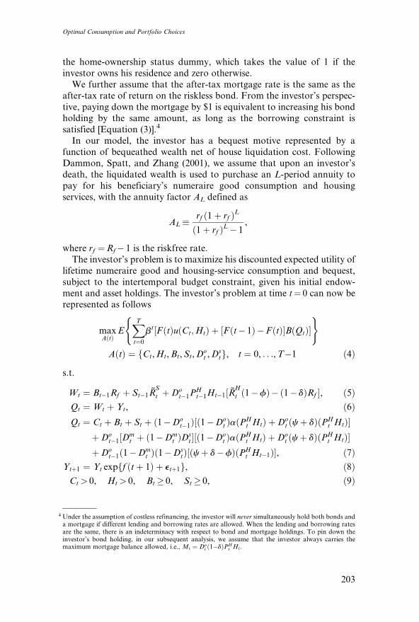
resources and labor income.Figure 1a shows the investor’s optimal housing tenure choice as a

function of the investor’s beginning-of-period net-worth–labor-income

ratio and the investor’s age. The solid curve represents the net-worth–

labor-income ratio trigger bound of owning versus renting. At a given

age, the investor with a high net-worth–labor-income ratio purchases a

house, while the investor with a low net-worth–labor-income ratio

chooses to rent. To own a house, the investor needs to meet the initial

down payment requirement and also satisfy subsequent home equityrequirements using his wealth on hand. An investor with a high net-

worth–labor-income ratio is less liquidity-constrained and can afford a

house closer to his desired size. Therefore, he expects to stay in the house

longer to reduce liquidation cost and is in a better position to benefit

from home ownership.11

Furthermore, the net-worth–labor-income ratio trigger bound

decreases in the age of the investor before the investor reaches his late

forties and increases thereafter. It then sharply declines as the investorapproaches retirement and his labor income is drastically reduced. After

retirement, the trigger bound monotonically increases in investor age. The

level of the trigger bound is determined primarily by the investor’s earn-

ings profile before retirement and bequest motive afterward. A young

investor has a high present value of labor income and wishes to own a

large house relative to his current labor income in order to smooth inter-

temporal housing services andminimize house liquidation cost. Therefore,

11 For the baseline case, the per-period user cost of home ownership— the sum of per-period maintenancecost, mortgage cost, and the opportunity cost of home equity, minus housing appreciation— is lowerthan the per-period cost of renting a similar property. Another possible modeling approach to inducehome ownership is through consumption motives— the investor derives higher utility from owning thanrenting the same property—by assigning a higher housing preference parameter for owning a houseversus renting. We solved a model in which v¼ 0.20 if housing services are acquired through renting andv¼ 0.25 if the investor owns his home, while per-period rental and owning costs are the same. The resultsare qualitatively very similar.


208

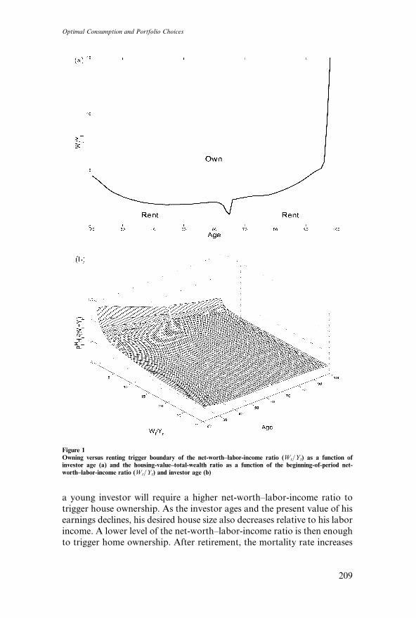
a young investor will require a higher net-worth–labor-income ratio to

trigger house ownership. As the investor ages and the present value of his

earnings declines, his desired house size also decreases relative to his labor

income. A lower level of the net-worth–labor-income ratio is then enough

to trigger home ownership. After retirement, the mortality rate increases

Figure 1Owning versus renting trigger boundary of the net-worth–labor-income ratio (Wt=Yt) as a function ofinvestor age (a) and the housing-value–total-wealth ratio as a function of the beginning-of-period net-worth–labor-income ratio (Wt=Yt) and investor age (b)


209

rapidly and the bequest motive gradually dominates the investor’s housing

decision. Because the investor derives utility from bequeathing his wealth

net of house liquidation cost, he is reluctant to purchase a house unless his

net-worth–labor-income ratio is so high that the additional benefit of

owning a house outweighs the cost of liquidation at the time of death.As the investor ages and death is proximate, the probability of incurring

liquidation cost also increases. The net-worth–labor-income ratio trigger

bound thus increases. Indeed, at very advanced ages, the investor always

rents housing services to avoid liquidation cost.

Figure 1b shows the fraction of wealth (the sum of net worth and current

labor income) allocated to housing as a function of the beginning-of-

period net-worth–labor-income ratio and the age of the investor. At a

given age, the investor spends less on housing services (either renting orowning) as his net-worth–labor-income ratio increases. The investor’s

expenditure on housing services decreases as the investor ages. This is

primarily driven by the gradual realization of the investor’s earning power

over his life cycle and is consistent with the permanent income hypothesis.

At a low net-worth–labor-income ratio, his labor income accounts for a

relatively large fraction of his spendable resources. The investor thus

spends a higher fraction of his wealth on housing services. Analogously,

when the investor’s net-worth–labor-income ratio is high and his laborincome accounts for a small fraction of his spendable resources, the

investor allocates a relatively small fraction of his wealth to housing

services.

On the trigger bound of owning versus renting, the investor consumes

more housing services when he owns a house than when he rents. This can

be explained as follows. Intratemporally, the investor will equate the

marginal utility of an additional dollar spent either on housing services

or on numeraire good consumption. Because renting is more expensivethan owning per unit of housing services, the investor consumes less

housing services relative to the numeraire good when renting than when

owning. The overall pattern of the investor’s numeraire good consump-

tion (figure not shown) is very similar to the investor’s housing-services

consumption. In contrast to his housing-consumption behavior, on the

trigger bound of owning versus renting, the investor consumes slightly

more numeraire good when renting than when owning. This reflects

the substitution effect of the numeraire good for housing services.We now discuss the investor’s investment decision. When the investor

chooses to rent housing services for the current period, all his net worth is

in the form of liquid financial assets: bonds and stocks. If the investor

chooses to own a house, a fraction of his net worth is held instead in

illiquid home equity. We therefore make a distinction between an inves-

tor’s liquid financial portfolio (bonds and stocks) and net worth (bonds,

stocks, and home equity).


210

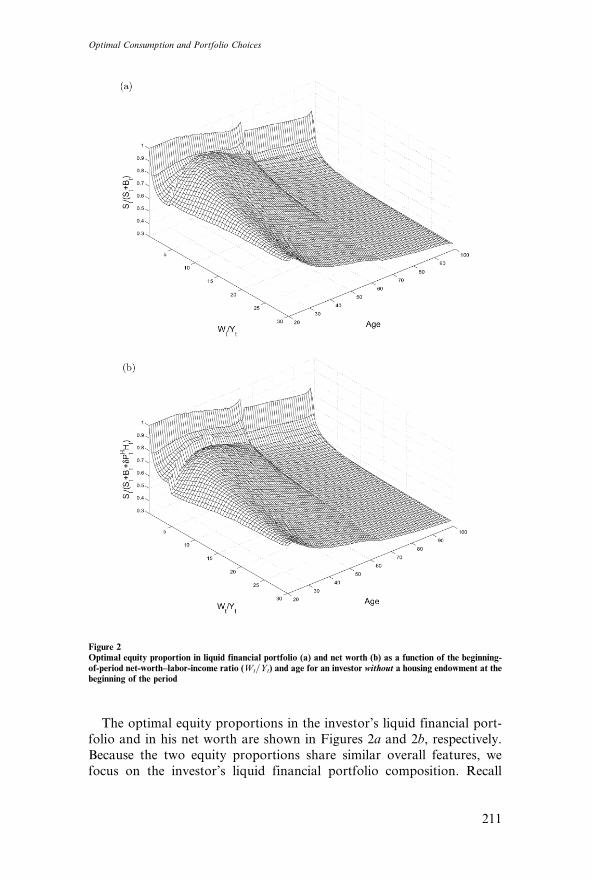
The optimal equity proportions in the investor’s liquid financial port-

folio and in his net worth are shown in Figures 2a and 2b, respectively.

Because the two equity proportions share similar overall features, we

focus on the investor’s liquid financial portfolio composition. Recall

Figure 2Optimal equity proportion in liquid financial portfolio (a) and net worth (b) as a function of the beginning-of-period net-worth–labor-income ratio (Wt=Yt) and age for an investor without a housing endowment at thebeginning of the period


211

that the investor rents housing services for liquidity reasons when his

beginning-of-period net-worth–labor-income ratio is low. As a renter,

the investor’s equity proportion can reach a very high level (close to

100%) and declines as the net-worth–labor-income ratio increases. This

is consistent with the findings regarding equity proportion levels in aneconomy without risky housing [see Jagannathan and Kocherlakota

(1996), Heaton and Lucas (2000b), and Cocco, Gomes, and Maenhout

(2004), among others]. It can be attributed to the fact that the presence of

labor income allows the investor to better diversify his exposure to equity

risk and crowds out riskless bond holding. When the investor owns a

house, his optimal equity proportion in the liquid financial portfolio is

hump-shaped in both the net-worth–labor-income ratio and age. Further,

the investor age at which the homeowner’s equity proportion peaks isinversely related to the investor’s net-worth–labor-income ratio. Two

effects contribute to the above observations. First, as the investor ages

or as his net-worth–labor-income ratio increases, the present value of his

lifetime earnings decreases relative to his net worth. Since the investor’s

labor income is a close substitute for bonds, the declining present value of

earnings leads the investor to increase his bond holdings and reduce his

stock holdings. Second, at very young ages or at very low levels of the net-

worth–labor-income ratio, homeowners are severely liquidity-constraineddue to the collateral requirements associated with housing. To alleviate

the liquidity concern, the investor tilts his liquid financial portfolio toward

safe assets.

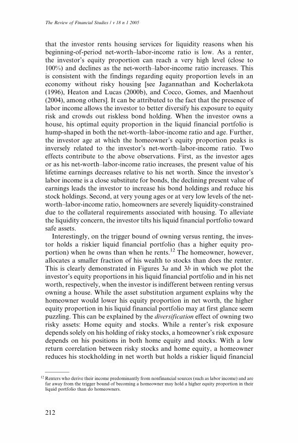
Interestingly, on the trigger bound of owning versus renting, the inves-

tor holds a riskier liquid financial portfolio (has a higher equity pro-

portion) when he owns than when he rents.12 The homeowner, however,

allocates a smaller fraction of his wealth to stocks than does the renter.

This is clearly demonstrated in Figures 3a and 3b in which we plot theinvestor’s equity proportions in his liquid financial portfolio and in his net

worth, respectively, when the investor is indifferent between renting versus

owning a house. While the asset substitution argument explains why the

homeowner would lower his equity proportion in net worth, the higher

equity proportion in his liquid financial portfolio may at first glance seem

puzzling. This can be explained by the diversification effect of owning two

risky assets: Home equity and stocks. While a renter’s risk exposure

depends solely on his holding of risky stocks, a homeowner’s risk exposuredepends on his positions in both home equity and stocks. With a low

return correlation between risky stocks and home equity, a homeowner

reduces his stockholding in net worth but holds a riskier liquid financial

12 Renters who derive their income predominantly from nonfinancial sources (such as labor income) and arefar away from the trigger bound of becoming a homeowner may hold a higher equity proportion in theirliquid portfolio than do homeowners.


212

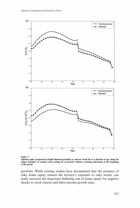
portfolio. While existing studies have documented that the presence of

risky home equity reduces the investor’s exposure to risky stocks, our

study uncovers the important buffering role of home equity for negative

shocks to stock returns and labor-income growth rates.

20 30 40 50 60 70 80 90 1000.2

0.3

0.4

0.5

0.6

0.7

0.8

0.9

1

Age

St/(S

t+Bt)

HomeownerRenter

(a)

(b)

20 30 40 50 60 70 80 90 1000.2

0.3

0.4

0.5

0.6

0.7

0.8

0.9

1

Age

St/(S

t+Bt+δ

PtHH

t)

HomeownerRenter

Figure 3Optimal equity proportion in liquid financial portfolio (a) and net worth (b) as a function of age along thetrigger boundary of owning versus renting for an investor without a housing endowment at the beginningof the period


213

2.2 Optimal consumption and investment policies with a housing

endowment

Our discussions so far have focused on the optimal policies for the

investor who does not own a house at the beginning of the current period

and can costlessly adjust his housing services, numeraire good consump-tion, and stock and bond holdings to their optimal levels. However, for an

investor who owns an existing house, the value of his existing house

also affects his consumption and portfolio decisions.

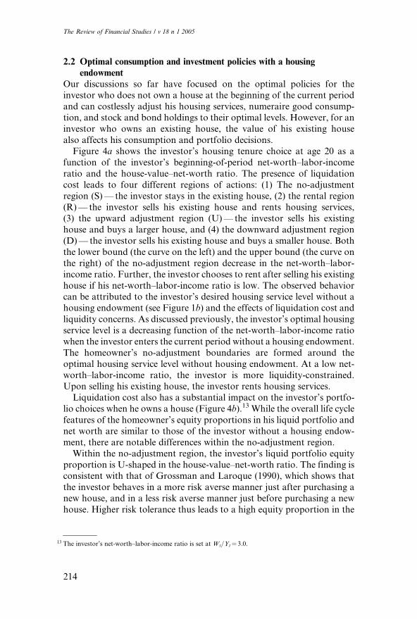
Figure 4a shows the investor’s housing tenure choice at age 20 as a

function of the investor’s beginning-of-period net-worth–labor-income

ratio and the house-value–net-worth ratio. The presence of liquidation

cost leads to four different regions of actions: (1) The no-adjustment

region (S)— the investor stays in the existing house, (2) the rental region(R)— the investor sells his existing house and rents housing services,

(3) the upward adjustment region (U)— the investor sells his existing

house and buys a larger house, and (4) the downward adjustment region

(D)— the investor sells his existing house and buys a smaller house. Both

the lower bound (the curve on the left) and the upper bound (the curve on

the right) of the no-adjustment region decrease in the net-worth–labor-

income ratio. Further, the investor chooses to rent after selling his existing

house if his net-worth–labor-income ratio is low. The observed behaviorcan be attributed to the investor’s desired housing service level without a

housing endowment (see Figure 1b) and the effects of liquidation cost and

liquidity concerns. As discussed previously, the investor’s optimal housing

service level is a decreasing function of the net-worth–labor-income ratio

when the investor enters the current period without a housing endowment.

The homeowner’s no-adjustment boundaries are formed around the

optimal housing service level without housing endowment. At a low net-

worth–labor-income ratio, the investor is more liquidity-constrained.Upon selling his existing house, the investor rents housing services.

Liquidation cost also has a substantial impact on the investor’s portfo-

lio choices when he owns a house (Figure 4b).13 While the overall life cycle

features of the homeowner’s equity proportions in his liquid portfolio and

net worth are similar to those of the investor without a housing endow-

ment, there are notable differences within the no-adjustment region.

Within the no-adjustment region, the investor’s liquid portfolio equity

proportion is U-shaped in the house-value–net-worth ratio. The finding isconsistent with that of Grossman and Laroque (1990), which shows that

the investor behaves in a more risk averse manner just after purchasing a

new house, and in a less risk averse manner just before purchasing a new

house. Higher risk tolerance thus leads to a high equity proportion in the

13 The investor’s net-worth–labor-income ratio is set at Wt=Yt¼ 3.0.


214

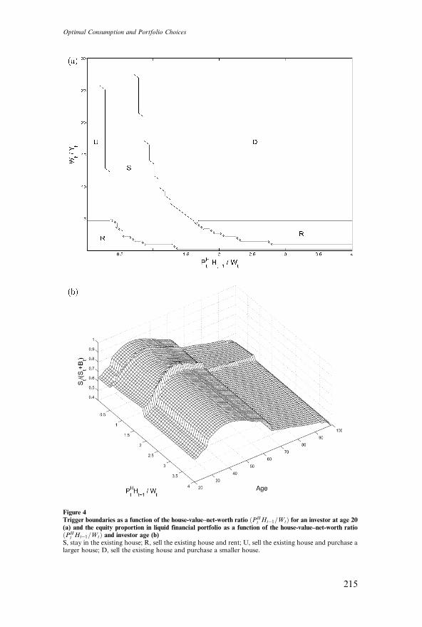
Figure 4Trigger boundaries as a function of the house-value–net-worth ratio ðPH

t Ht�1=WtÞ for an investor at age 20(a) and the equity proportion in liquid financial portfolio as a function of the house-value–net-worth ratioðPH

t Ht�1=WtÞ and investor age (b)S, stay in the existing house; R, sell the existing house and rent; U, sell the existing house and purchase alarger house; D, sell the existing house and purchase a smaller house.


215

investor’s liquid financial portfolio near the trigger bounds. When his

house-value–net-worth ratio is close to the optimal level without a hous-

ing endowment, the investor holds a safer liquid portfolio to reduce

deviations from the ‘‘target’’ level of the house-value–net-worth ratio.

In our model, while the lower risk aversion on the trigger bounds leadsto a riskier liquid portfolio, the investor’s net worth equity proportion

decreases in the house-value—net worth ratio (figure not shown). This is

attributable to the model’s collateral requirements. When the investor

refrains from selling a house larger than his desired size, he holds more

home equity than the optimal level without a housing endowment. As a

result, the investor reduces his liquid financial asset holdings, including

stocks, to finance home equity.

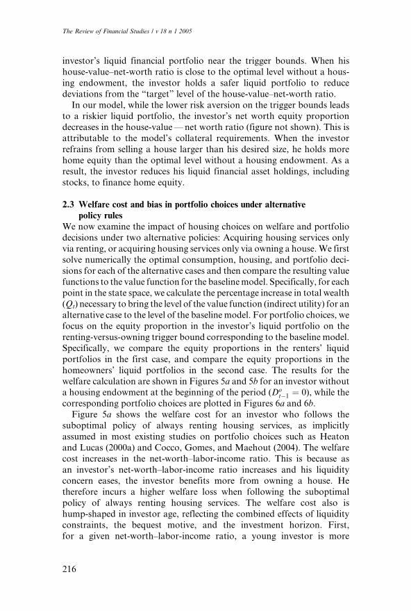
2.3 Welfare cost and bias in portfolio choices under alternativepolicy rules

We now examine the impact of housing choices on welfare and portfolio

decisions under two alternative policies: Acquiring housing services only

via renting, or acquiring housing services only via owning a house.We first

solve numerically the optimal consumption, housing, and portfolio deci-

sions for each of the alternative cases and then compare the resulting value

functions to the value function for the baselinemodel. Specifically, for each

point in the state space, we calculate the percentage increase in total wealth(Qt) necessary to bring the level of the value function (indirect utility) for an

alternative case to the level of the baseline model. For portfolio choices, we

focus on the equity proportion in the investor’s liquid portfolio on the

renting-versus-owning trigger bound corresponding to the baseline model.

Specifically, we compare the equity proportions in the renters’ liquid

portfolios in the first case, and compare the equity proportions in the

homeowners’ liquid portfolios in the second case. The results for the

welfare calculation are shown in Figures 5a and 5b for an investor withouta housing endowment at the beginning of the period (Do

t�1 ¼ 0), while the

corresponding portfolio choices are plotted in Figures 6a and 6b.

Figure 5a shows the welfare cost for an investor who follows the

suboptimal policy of always renting housing services, as implicitly

assumed in most existing studies on portfolio choices such as Heaton

and Lucas (2000a) and Cocco, Gomes, and Maehout (2004). The welfare

cost increases in the net-worth–labor-income ratio. This is because as

an investor’s net-worth–labor-income ratio increases and his liquidityconcern eases, the investor benefits more from owning a house. He

therefore incurs a higher welfare loss when following the suboptimal

policy of always renting housing services. The welfare cost also is

hump-shaped in investor age, reflecting the combined effects of liquidity

constraints, the bequest motive, and the investment horizon. First,

for a given net-worth–labor-income ratio, a young investor is more


216

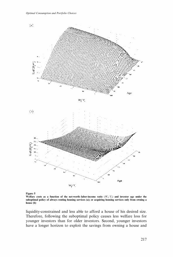
liquidity-constrained and less able to afford a house of his desired size.

Therefore, following the suboptimal policy causes less welfare loss for

younger investors than for older investors. Second, younger investors

have a longer horizon to exploit the savings from owning a house and

Figure 5Welfare costs as a function of the net-worth–labor-income ratio (Wt=Yt) and investor age under thesuboptimal policy of always renting housing services (a); or acquiring housing services only from owning ahouse (b)


217

thus incur higher welfare costs when they always rent housing services.

This horizon effect thus declines in age. Further, as the investor

approaches the terminal date, he also refrains from owning a house to

avoid house liquidation cost at death. The bequest motive thus reinforces

20 30 40 50 60 70 80 90 1000.2

0.3

0.4

0.5

0.6

0.7

0.8

0.9

1

Age

St/(S

t+Bt)

Renter w/ Future OwningRenter w/o Future Owning

(a)

20 30 40 50 60 70 80 90 1000.2

0.3

0.4

0.5

0.6

0.7

0.8

0.9

1

Age

St/(S

t+Bt)

Owner w/ Future RentingOwner w/o Future Renting

(b)

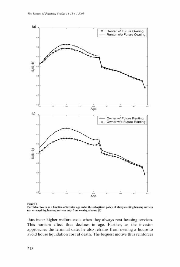
Figure 6Portfolio choices as a function of investor age under the suboptimal policy of always renting housing services(a); or acquiring housing services only from owning a house (b)


218

the horizon effect at advanced ages. Overall, the welfare cost of forgoing

the opportunity to own a house is quite high for the investor with a high

net worth. For example, for an investor with a net worth that is 30 times

his annual labor income, the welfare cost is almost 8% of his current

wealth, reflecting the large lifetime benefit of home ownership.The investor’s portfolio choice also is substantially affected if the inves-

tor follows the suboptimal policy of always renting housing services

(Figure 6a). Specifically, relative to the optimal portfolio choice with

home ownership, the equity proportion is biased upward. The bias reflects

the tradeoff between earning a higher equity premium and benefiting from

being a homeowner. In the baseline model, the investor holds a safer liquid

portfolio while saving for initial down payment to purchase a house. Since

the investor under the alternative policy will never own a house, he takes ahigher risk in his liquid financial portfolio by allocating a larger fraction

of his liquid financial investments to stocks. For our parameter values, the

gap between the equity proportions of the optimal and suboptimal poli-

cies’ liquid financial portfolios reaches a peak of 4.3% for the investor in

his early forties. Our findings also imply that studies excluding home

ownership market offer reasonable approximations to the optimal con-

sumption and portfolio policies only when the investor’s net worth

remains very low throughout his lifetime and the investor never becomesa homeowner. Yet, the same studies usually predict that the investor

accumulates a high net worth relative to his labor income, at least at

some stages of his life cycle.

Since renting is the only alternative to owning, the qualitative features

of welfare cost arising from always owning a house are the opposite of

those arising from always renting housing services. The welfare cost

decreases in the investor’s net-worth–labor-income ratio and is U-shaped

in the investor’s age (see Figure 5b). Strikingly, the welfare cost of follow-ing the suboptimal policy of forgoing the opportunity to rent housing

services, as in Cocco (2004), can be very large for an investor with a low

net-worth–labor-income ratio or an investor approaching the terminal

date. This reflects the critical role played by the house rental market in

allowing investors to smooth housing consumption and avoiding house

liquidation cost. For instance, for an investor with little net worth or an

investor in his late nineties, the welfare cost can amount to more than 25%

of his total wealth. It is intuitively clear that the investor who rents in thebaseline model would be forced under the suboptimal policy to purchase a

small house, which would provide far fewer services than his rental house

and would likely be liquidated soon after some wealth accumulation or

upon the investor’s death. This finding implies that excluding the house

rental market in studies of illiquid risky housing decisions may lead to

distorted housing choices for investors facing severe liquidity constraints

or investors at advanced ages.


219

The lack of rental opportunities also drastically alters the investor’s

portfolio choices (see Figure 6b). Specifically, compared to the

optimal portfolio choice in an economy with a rental market, the

investor’s liquid portfolio stockholding is substantially biased downward.

This can be explained by the excessively precautionary motive to holdbonds. Under the suboptimal policy, the investor acquires housing

services only from owning a house. The homeowner thus has an incentive

to hold more safe assets—bonds— in order to meet his subsequent

liquidity constraints and to reduce the frequency of house turnover. For

our parameter values, the equity proportion gap in the liquid financial

portfolios reaches a peak of 10.3% for an investor in his early forties.

2.4 Hedging demand induced by housing price risk and the effect of

moving shocksIn this section, we first examine the hedging demand for stocks induced by

housing price risk when stock returns and housing returns are positively

correlated. We then consider the effect of an exogenous moving shock on

an investor’s housing and portfolio choices.

The net-worth–labor-income ratio trigger bound of owning versus rent-

ing is shifted upward (Figure 7a), if stock returns and housing returns are

positively correlated (rH,S¼ 0.2), indicating the investor’s need to accu-

mulate more net worth before purchasing a house. This reflects the pre-cautionary motive to save more in order to alleviate potential liquidity

concerns caused by the positive comovement between the stock market

and the housing market.

Since the investor’s net-worth–labor-income ratio trigger bound is

higher for a positive stock- and housing-return correlation, we plot the

homeowner’s liquid portfolio equity proportion on the trigger bound

corresponding to a positive stock- and housing-return correlation

(Figure 7b) and the renter’s equity proportion on the trigger boundcorresponding to a zero stock- and housing-return correlation (Figure 7c).

Because the hedging demand for stocks induced by housing price risk is

zero when stock returns and housing returns are uncorrelated ( rH,S¼ 0),

the gap in equity proportions thus reflects the hedging demand for stocks

attributable to the correlation between stock returns and housing returns.

Further, since a homeowner holds a long position in housing assets, the

hedging demand should reduce the homeowner’s stockholding when the

stock- and housing-returns are positively correlated. Indeed, compared tothe baseline case, the homeowner’s equity proportion is notably lower in

the case with a positive stock- and housing-return correlation. For our

parameter values, the homeowner’s liquid portfolio equity proportion can

be reduced by as much as 7.0%. Interestingly, for the renter, the hedging

demand increases the investor’s equity proportion when the stock returns

and housing returns are positively correlated. For our parameter values,


220

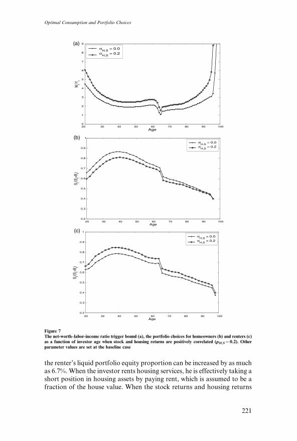
the renter’s liquid portfolio equity proportion can be increased by as much

as 6.7%.When the investor rents housing services, he is effectively taking a

short position in housing assets by paying rent, which is assumed to be a

fraction of the house value. When the stock returns and housing returns

20 30 40 50 60 70 80 90 1000

1

2

3

4

5

6

7

8

9

Age

Wt/Y

t

σH,S

= 0.0σ

H,S = 0.2

(a)

20 30 40 50 60 70 80 90 1000.2

0.3

0.4

0.5

0.6

0.7

0.8

0.9

1

Age

S t/(St+B

t)

σH,S

= 0.0σ

H,S = 0.2

(b)

20 30 40 50 60 70 80 90 1000.2

0.3

0.4

0.5

0.6

0.7

0.8

0.9

1

Age

S t/(St+B

t)

σH,S

= 0.0σ

H,S = 0.2

(c)

Figure 7The net-worth–labor-income ratio trigger bound (a), the portfolio choices for homeowners (b) and renters (c)as a function of investor age when stock and housing returns are positively correlated (rH,S¼ 0.2). Otherparameter values are set at the baseline case


221

are positively correlated, investing in stocks helps the renter to hedge

against fluctuations in his future rent and house down payment.

When facing an exogenous moving shock, investors become home-

owners at higher levels of the net-worth–labor-income ratio (data not

shown). Young investors, in particular, purchase a house only after theyhave accumulated substantially more net worth than in the case without

the moving shock. This is to be expected and is caused by high housing

liquidation cost and the fact that young investors have higher probabilities

of moving. However, the exogenous moving shock has only a small effect

on investors’ portfolio choices. For both homeowners and renters,

the optimal portfolios consist of slightly more equity with a positive

probability of a moving shock (data not shown). This captures the

reduced incentive to invest conservatively when there is a reduced homeownership benefit.

2.5 Comparative static analysis

In this section, we provide comparative static results by varying the house

maintenance cost, the riskiness of the housing return, the correlation

between the housing return and the labor-income growth rate, and the

investor’s calibrated labor-income profile. Our discussions will focus on

the housing tenure decision and portfolio choices for an investor entering

the current period without a housing endowment.The overall qualitative features of the trigger bounds for these cases are

quite similar to those of the trigger bound in the baseline case (data not

shown). However, there are some notable quantitative differences. Specif-

ically, increasing the house maintenance cost shifts the trigger bound

upward for all ages, indicating that the investor accumulates more net

worth before purchasing a house when the benefit of home ownership is

lower. Eliminating the housing-return risk or the positive correlation

between housing return and the labor-income growth rate, however, low-ers the trigger bound before retirement. This is because the borrowing

constraint, often binding when there is a negative housing-return shock, is

now relaxed. Since zero housing risk also leads to zero correlation between

housing return and labor-income growth rate, removing housing risk is

more effective in inducing home ownership than eliminating a positive

correlation between these factors. Unlike the cases discussed above, the

effect of a changing labor-income profile on trigger bound is not mono-

tonic. A high school graduate requires a lower net-worth–labor-incomeratio to trigger home ownership at young ages (prior to 38 years), yet a

higher net-worth–labor-income ratio thereafter until he reaches retire-

ment. This reflects the difference in labor-income profiles between college

and high school graduates during the working years. On one hand, at

young ages, the higher growth rate of a college graduate’s labor income

leads to a larger desired house relative to his labor-income level, which


222

requires more wealth on hand to meet the house collateral constraint. On

the other hand, in middle age, the faster decline in the labor income of a

college graduate results in a smaller desired house relative to current labor

income, which explains the reversal in the trigger level of the net-worth–

labor-income ratio.For all four alternative scenarios investigated in this section, the inves-

tor’s liquid portfolio equity proportions exhibit similar patterns to the

baseline case (data not shown). They are all hump-shaped before retire-

ment and steadily declining thereafter. Yet, some interesting differences

emerge. First, at a higher maintenance cost, the investor stays as a renter

much longer and waits until his mid-thirties to purchase a house. The

investor thus holds fewer stocks in his liquid portfolio due to a renter’s

lack of diversification. However, once becoming a homeowner, the inves-tor chooses a riskier liquid portfolio than the baseline case. This reflects

the fact that with a smaller home ownership benefit, renting is a less

onerous alternative to owning, which alleviates the impact of the negative

shock to wealth and reduces the homeowner’s precautionary motive to

hold safe assets. Second, the elimination of housing risk or of the positive

correlation between housing risk and the labor-income growth rate allows

the investor to take more risk in his liquid portfolio. This reflects the fact

that the investor can now hold a greater amount of stock without increas-ing his overall risk exposure. The effect of zero correlation is, however,

much smaller than that of zero housing risk. Last, consistent with Cocco,

Gomes, and Maenhout (2004), the peak of the investor’s liquid portfolio

equity proportion occurs much earlier for a high school graduate, reflect-

ing the differences in labor-income profiles between investors with differ-

ent educational attainments.

2.6 Simulation analysis

Given the investor’s optimal decision rules defined on the state space,we can obtain time-series profiles of investors’ optimal housing services,

numeraire good consumption, and portfolio allocations using simulation.

Specifically, we first simulate stock return, housing return, and labor-

income growth rate based on a serially uncorrelated markov process

with two outcomes for each variable. We then use the optimal policy

rules from our state-space solution to calculate the investor’s optimal

numeraire good consumption, housing, and portfolio choices. Home

ownership status, the net worth–labor-income ratio, and the housing-value–wealth ratio are updated each period to determine the investor’s

optimal decisions for the next period. The time-series profiles of the

optimal decisions are generated by repeating the calculation from t¼ 0

(age 20) to t¼ 80 (age 100).

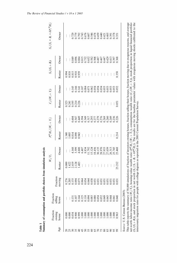
In Table 1, we summarize the results for 50,000 simulation trials

(or 50,000 time-series profiles) for the baseline parameter values with a


223

Table

1Summary

ofconsumptionandportfoliochoices

from

simulationanalysis

Age

Fraction

owning

house

Fraction

selling

house

Fraction

moving

Wt=Yt

PH tH

t=ðW

tþY

tÞCt=(W

tþYt)

St=(S

tþBt)

St=ðS

t+Bt+dPtHH

tÞ

Renter

Owner

Renter

Owner

Renter

Owner

Renter

Owner

Owner

20

0.000

—0.276

0.000

—1.340

—0.323

—0.994

——

25

0.000

—0.205

1.622

—1.005

—0.241

—0.818

——

30

0.034

0.131

0.135

2.419

4.168

0.814

0.604

0.195

0.145

0.815

0.849

0.729

35

0.900

0.107

0.094

2.124

3.599

0.890

0.547

0.214

0.166

0.910

0.896

0.779

40

0.999

0.144

0.075

1.483

4.608

0.943

0.449

0.226

0.141

0.939

0.884

0.792

45

1.000

0.125

0.064

—6.407

—0.394

—0.107

—0.815

0.743

50

1.000

0.110

0.054

—8.834

—0.349

—0.084

—0.732

0.676

55

1.000

0.094

0.044

—11.792

—0.317

—0.071

—0.652

0.607

60

1.000

0.085

0.038

—15.124

—0.293

—0.062

—0.582

0.546

65

1.000

0.080

0.031

—18.456

—0.277

—0.054

—0.508

0.478

70

1.000

0.054

0.031

—30.135

—0.279

—0.054

—0.487

0.459

75

1.000

0.052

0.031

—28.970

—0.276

—0.054

—0.467

0.440

80

1.000

0.049

0.031

—27.933

—0.269

—0.053

—0.447

0.421

85

1.000

0.045

0.031

—27.039

—0.260

—0.053

—0.429

0.405

90

1.000

0.044

0.031

—26.313

—0.249

—0.053

—0.413

0.391

95

1.000

0.041

0.031

—25.745

—0.236

—0.053

—0.397

0.378

99

0.963

0.048

0.031

25.212

25.468

0.214

0.226

0.051

0.052

0.358

0.368

0.351

Source:

U.S.CensusBureau(2003).

Thistablereportsthesummary

of50,000simulationsoffractionofinvestors

owninghouses,fractionsellingtheirhouses,fractionmovingdueto

exogenousreasons,andaverage

net-w

orth–labor-incomeratio(W

t=Yt),housing-value–wealthratio(P

H tH

t=ðW

tþY

tÞ),consumption–wealthratio(C

t=(W

tþYt)),stock

proportionin

liquid

financialportfolio

(St=(S

tþBt)),andstock

proportionin

net

worth(S

t=ðS

tþBtþdPH tH

tÞ).Theresultsare

forthebaselineparameter

values

withexogenousmovingshockscalibratedto

the

intercounty

migrationratesforpeoplewithcollegedegrees

asreported

inthe2001CurrentPopulationSurvey.


224

positive exogenous moving shock calibrated to the intercounty migration

rates of college graduates.14 The simulation begins with renters with zero

initial net worth, so it depicts the time-series profiles of typical college

graduates freshly out of school and starting to receive labor income. In the

table, we show the average age profiles for the fraction of investors owningand selling their houses, the fraction of investors experiencing exogenous

moving shocks, the net-worth–labor-income ratio, house value and

numeraire good consumption as a proportion of total wealth (net worth

plus labor income), and equity proportions in both the liquid portfolio

and net worth. We further separate the decisions of homeowners from

renters whenever it is feasible.

Investors purchase houses early in their lifetime after they accumulate

enough net worth to take advantage of home ownership. The fraction ofinvestors owning their first home increases with investor age until the mid-

forties, when almost all investors have become homeowners. After age 95,

however, the mortality rates are so high that upon selling their house

investors may choose to move into a rental home to prepare for bequeath-

ing their wealth. The house-selling rate among existing homeowners is in

general very low, reflecting the deterrent effect of liquidation cost on

home-selling decisions. Before age 35, the home-selling rate largely tracks

the probability of incurring the exogenous moving shock and declineswith age. The rate then picks up and reaches a peak level of 14.4% at

age 40, as more homeowners adjust their housing service levels. The selling

rate declines thereafter, reflecting a decrease in the probability of exoge-

nous moving as well as the fact that at this stage of their lives investors are

more capable of purchasing a house matching their lifetime consumption

level and hence have no need to make frequent adjustments. The cumula-

tive house turnover is about 5.06, implying that an investor sells his house

about five times during his lifetime.The average housing-value–wealth ratio exhibits a U-shape for renters

between age 20 and the early forties, but it steadily declines for home-

owners as they age. This is attributed to the time-series behavior of the

investor’s net-worth–labor-income ratio and the fact that investors with a

high net-worth–income ratio become homeowners earlier. As an investor

ages, his human capital is gradually realized and saved in the form of

liquid financial assets. This leads to the initial decline in the housing-

value–wealth ratio. However, a young renter who experiences a sequenceof positive shocks to stock returns and labor-income growth rates

will soon accumulate enough net worth to become a homeowner. So

the endogenous housing tenure choice will reduce the average net

14 We choose to report the simulation results for the case with a positive probability of exogenous moving sothat we can better match the patterns of home ownership and house-selling rates observed in the data inour empirical analysis.


225

worth–labor-income ratio for the renters left behind. The lower net

worth–labor-income ratio in turn increases the renters’ average housing-

related expenditures. After age 40, most investors become homeowners

and enter their prime time of saving. As they accumulate more net worth,

the housing-value–net-worth ratio declines monotonically. For the samereason, the average fraction of total wealth allocated to numeraire good

consumption is U-shaped in age for young renters and decreasing in age

for homeowners. When renting, investors spend on average 32.3% of their

current wealth on numeraire good consumption at age 20. The percentage

then decreases to 19.5% by the time the investors reach age 30. It then goes

back up to about 22.6%. When owning, investors allocate 16.6% of their

total wealth to numeraire good consumption at age 35, and the proportion

gradually reduces to 5.4% at age 65 and beyond. On average, renters spenda higher fraction of their current wealth on numeraire good consumption

than homeowners, primarily because of their lower average net-worth–

labor-income ratio.

The hump-shaped average net-worth–labor-income ratio for young

renters leads to a U-shaped portfolio allocation pattern (Table 1). The

investor holds a high equity proportion of 99.4% at age 20 due to the high

present value of human capital at this age. As the investor saves his labor

income in the form of financial assets and approaches the trigger boundof becoming a homeowner, his equity proportion declines. Saving for a

housing down payment is another reason for a young investor to tilt

his savings toward safer assets. Once a renter successfully accumulates

enough wealth, he becomes a homeowner and lowers the equity propor-

tion in his net worth by substituting risky housing assets for risky stocks to

control the overall risk exposure. In the meantime, he also raises the equity

proportion in his liquid financial portfolio to take advantage of the

diversification benefit from the low correlation between housing returnsand stock returns. As the investor ages, the equity proportions in both his

liquid portfolio and his net worth decline rapidly as he realizes his earning

ability and saves more in the form of financial assets. Among investors

over age 35 who are still unable to accumulate enough net worth to buy a

house, the average stock investment increases due to their higher earnings

potential (relative to their wealth on hand). From age 35 to 40, the average

equity proportion in the renter’s liquid portfolio is higher than that of

homeowners in the same age group.

3. Empirical Analysis of Household Portfolio Choices

In this section, we empirically investigate households’ portfolio choices in

the presence of risky housing using panel data. We focus on a household’s

stock investment as a proportion of either the household’s net worth or

its liquid financial asset holdings. We examine how a household’s stock


226

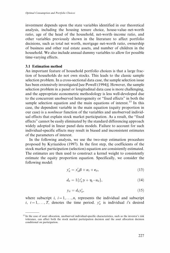
investment depends upon the state variables identified in our theoretical

analysis, including the housing tenure choice, house-value–net-worth

ratio, age of the head of the household, net-worth–income ratio, and

other variables previously shown in the literature to affect portfolio

decisions, such as total net worth, mortgage–net-worth ratio, ownershipof business and other real estate assets, and number of children in the

household. We also include annual dummy variables to allow for possible

time-varying effects.

3.1 Estimation method

An important feature of household portfolio choices is that a large frac-

tion of households do not own stocks. This leads to the classic sample

selection problem. In a cross-sectional data case, the sample selection issue

has been extensively investigated [see Powell (1994)]. However, the sampleselection problem in a panel or longitudinal data case is more challenging,

and the appropriate econometric methodology is less well-developed due

to the concurrent unobserved heterogeneity or ‘‘fixed effects’’ in both the

sample selection equation and the main equations of interest.15 In this

case, the dependent variable in the main equation (equity proportion in

our case) is a nonlinear function of the variables and unobserved individ-

ual effects that explain stock market participation. As a result, the ‘‘fixed

effects’’ cannot be easily eliminated by the standard differencing approachwidely adopted in linear panel data models. Failure to account for such

individual-specific effects may result in biased and inconsistent estimates

of the parameters of interest.

In the following analysis, we use the two-step estimation procedure

proposed by Kyriazidou (1997). In the first step, the coefficients of the

stock market participation (selection) equation are consistently estimated.

The estimates are then used to construct a kernel weight to consistently

estimate the equity proportion equation. Specifically, we consider thefollowing model:

y�it ¼ x0itbþ ai þ eit, ð13Þ

dit ¼ 1fz0itg þ hi�uitg, ð14Þ

yit ¼ dity�it, ð15Þ

where subscript i, i¼ 1, . . . , n, represents the individual and subscript

t, t¼ 1, . . . ,T, denotes the time period. y�it is individual i’s desired

15 In the case of asset allocation, unobserved individual-specific characteristics, such as the investor’s risktolerance, can affect both the stock market participation decision and the asset allocation decisionconditional on participation.


227

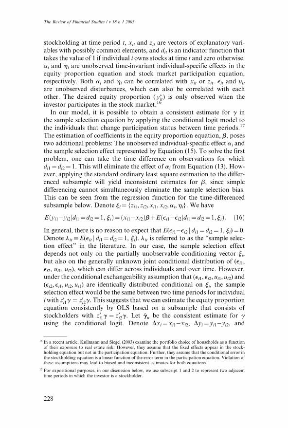
stockholding at time period t, xit and zit are vectors of explanatory vari-

ables with possibly common elements, and dit is an indicator function that

takes the value of 1 if individual i owns stocks at time t and zero otherwise.

ai and hi are unobserved time-invariant individual-specific effects in the

equity proportion equation and stock market participation equation,respectively. Both ai and hi can be correlated with xit or zit. eit and uitare unobserved disturbances, which can also be correlated with each

other. The desired equity proportion ( y�it) is only observed when the

investor participates in the stock market.16

In our model, it is possible to obtain a consistent estimate for g in

the sample selection equation by applying the conditional logit model to

the individuals that change participation status between time periods.17

The estimation of coefficients in the equity proportion equation, b, posestwo additional problems: The unobserved individual-specific effect ai and

the sample selection effect represented by Equation (15). To solve the first

problem, one can take the time difference on observations for which

di1¼ di2¼ 1. This will eliminate the effect of ai from Equation (13). How-

ever, applying the standard ordinary least square estimation to the differ-

enced subsample will yield inconsistent estimates for b, since simple

differencing cannot simultaneously eliminate the sample selection bias.

This can be seen from the regression function for the time-differencedsubsample below. Denote ji¼ {zi1, zi2, xi1, xi2,ai,hi}. We have

Eðyi1�yi2jdi1¼di2¼1, jiÞ¼ðxi1�xi2ÞbþEðei1�ei2jdi1¼di2¼1, jiÞ: ð16Þ

In general, there is no reason to expect that E(ei1�ei2 j di1¼ di2¼ 1, ji)¼ 0.

Denote lit�E(eit j di1¼ di2¼ 1, ji). lit is referred to as the ‘‘sample selec-

tion effect’’ in the literature. In our case, the sample selection effectdepends not only on the partially unobservable conditioning vector ji,

but also on the generally unknown joint conditional distribution of (ei1,

ei2, ui1, ui2), which can differ across individuals and over time. However,

under the conditional exchangeability assumption that (ei1, ei2, ui1, ui2) and

(ei2, ei1, ui2, ui1) are identically distributed conditional on ji, the sample

selection effect would be the same between two time periods for individual

iwith z0i1g ¼ z0i2g. This suggests that we can estimate the equity proportion

equation consistently by OLS based on a subsample that consists ofstockholders with z0i1g ¼ z0i2g. Let ggn be the consistent estimate for g

using the conditional logit. Denote Dxi¼ xi1�xi2, Dyi¼ yi1�yi2, and

16 In a recent article, Kullmann and Siegel (2003) examine the portfolio choice of households as a functionof their exposure to real estate risk. However, they assume that the fixed effects appear in the stock-holding equation but not in the participation equation. Further, they assume that the conditional error inthe stockholding equation is a linear function of the error term in the participation equation. Violation ofthese assumptions may lead to biased and inconsistent estimates for both equations.

17 For expositional purposes, in our discussion below, we use subscript 1 and 2 to represent two adjacenttime periods in which the investor is a stockholder.


228

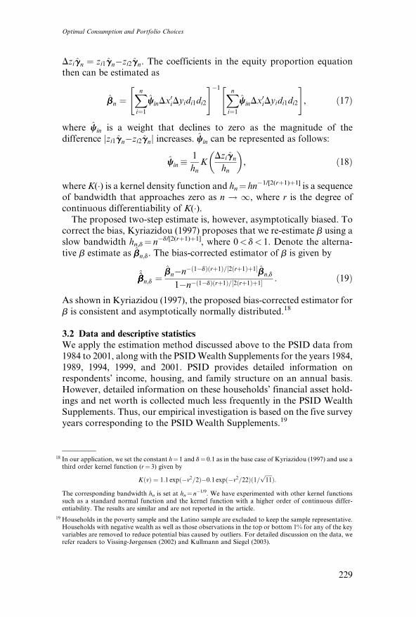
Dziggn ¼ zi1ggn�zi2ggn. The coefficients in the equity proportion equation

then can be estimated as

bbn ¼Xni¼1

ccinDx0iDyidi1di2

" #�1 Xni¼1

ccinDx0iDyidi1di2

" #, ð17Þ

where ccin is a weight that declines to zero as the magnitude of the

difference jzi1ggn�zi2ggnj increases. ccin can be represented as follows:

ccin �1

hnK

Dziggn

hn

� �, ð18Þ

where K(�) is a kernel density function and hn¼ hn�1/[2(rþ1)þ1] is a sequence

of bandwidth that approaches zero as n ! 1, where r is the degree of

continuous differentiability of K(�).The proposed two-step estimate is, however, asymptotically biased. To

correct the bias, Kyriazidou (1997) proposes that we re-estimate b using a

slow bandwidth hn,d¼ n�d/[2(rþ1)þ1], where 0< d< 1. Denote the alterna-

tive b estimate as bbn;d. The bias-corrected estimator of b is given by

^bbbbn;d ¼

bbn�n�ð1�dÞðrþ1Þ=½2ðrþ1Þþ1�bbn;d

1�n�ð1�dÞðrþ1Þ=½2ðrþ1Þþ1� : ð19Þ

As shown in Kyriazidou (1997), the proposed bias-corrected estimator for

b is consistent and asymptotically normally distributed.18

3.2 Data and descriptive statistics

We apply the estimation method discussed above to the PSID data from

1984 to 2001, along with the PSIDWealth Supplements for the years 1984,

1989, 1994, 1999, and 2001. PSID provides detailed information on

respondents’ income, housing, and family structure on an annual basis.However, detailed information on these households’ financial asset hold-

ings and net worth is collected much less frequently in the PSID Wealth

Supplements. Thus, our empirical investigation is based on the five survey

years corresponding to the PSID Wealth Supplements.19

18 In our application, we set the constant h¼ 1 and d¼ 0.1 as in the base case of Kyriazidou (1997) and use athird order kernel function (r¼ 3) given by

KðvÞ ¼ 1:1 expð�v2=2Þ�0:1 expð�v2=22Þð1=ffiffiffiffiffi11

pÞ:

The corresponding bandwidth hn is set at hn¼ n�1/9. We have experimented with other kernel functionssuch as a standard normal function and the kernel function with a higher order of continuous differ-entiability. The results are similar and are not reported in the article.

19 Households in the poverty sample and the Latino sample are excluded to keep the sample representative.Households with negative wealth as well as those observations in the top or bottom 1% for any of the keyvariables are removed to reduce potential bias caused by outliers. For detailed discussion on the data, werefer readers to Vissing-Jørgensen (2002) and Kullmann and Siegel (2003).


229

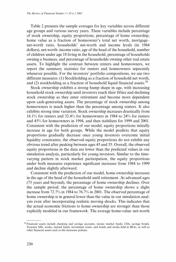
Table 2 presents the sample averages for key variables across different

age groups and various survey years. These variables include percentage

of stock ownership, equity proportions, percentage of home ownership,

home value as a fraction of homeowner’s total net worth, mortgage–

net-worth ratio, households’ net-worth and income levels (in 1984dollars), net-worth–income ratio, age of the head of the household, number

of children under age 18 living in the household, percentage of households

owning a business, and percentage of households owning other real estate

assets. To highlight the contrast between renters and homeowners, we

report the summary statistics for renters and homeowners separately

whenever possible. For the investors’ portfolio compositions, we use two

different measures: (1) Stockholding as a fraction of household net worth,

and (2) stockholding as a fraction of household liquid financial assets.20

Stock ownership exhibits a strong hump shape in age, with increasing

household stock ownership until investors reach their fifties and declining

stock ownership as they enter retirement and become more dependent

upon cash-generating assets. The percentage of stock ownership among

homeowners is much higher than the percentage among renters. It also

exhibits strong time variation. Stock ownership increases drastically from

16.1% for renters and 32.4% for homeowners in 1984 to 24% for renters

and 45% for homeowners in 1994, and then stabilizes for 1999 and 2001.Consistent with the prediction of our model, equity proportions initially

increase in age for both groups. While the model predicts that equity

proportions gradually decrease once young investors overcome initial

liquidity constraints, the observed equity proportions do not exhibit any

obvious trend after peaking between ages 45 and 55. Overall, the observed

equity proportions in the data are lower than the predicted values in our

simulation analysis, particularly for young investors. Similar to the time-

varying pattern in stock market participation, the equity proportionsunder both measures experience significant increases from 1984 to 1999

and decline slightly afterward.

Consistent with the prediction of our model, home ownership increases

in the age of the head of the household until retirement. At advanced ages

(75 years and beyond), the percentage of home ownership declines. Over

the sample period, the percentage of home ownership shows a slight

increase from 72.7% in 1984 to 76.7% in 2001. The observed percentage of

home ownership is in general lower than the value in our simulation anal-ysis even after incorporating realistic moving shocks. This indicates that

the actual economic frictions to home ownership are stronger than those

explicitly modeled in our framework. The average home-value–net-worth

20 Financial assets include checking and savings accounts, money market funds, CDs, savings bonds,Treasury bills, stocks, mutual funds, investment trusts, and bonds and stocks held in IRAs, as well asother financial assets such as life insurance policies.


230

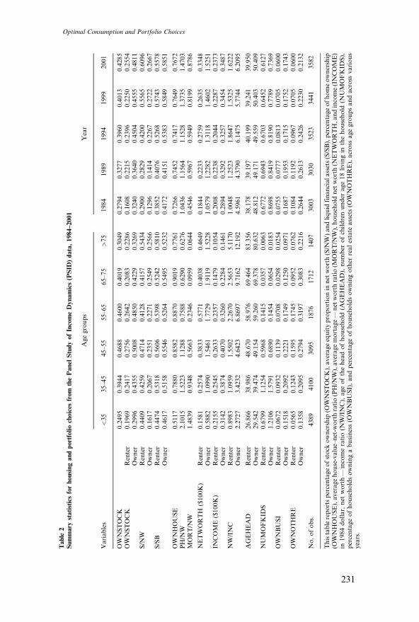
Table

2Summary

statisticsforhousingandportfoliochoices

from

thePanel

StudyofIncomeDynamics(PSID

)data,1984–2001

Agegroups

Year

Variables

<35

35–45

45–55

55–65

65–75

>75

1984

1989

1994

1999

2001

OWNSTOCK

0.2495

0.3944

0.4688

0.4600

0.4019

0.3049

0.2794

0.3277

0.3960

0.4013

0.4285

OWNSTOCK

Renter

0.1969

0.2417

0.2756

0.2642

0.2083

0.2286

0.1608

0.2215

0.2396

0.2250

0.2554

Owner

0.2996

0.4355

0.5008

0.4850

0.4229

0.3269

0.3240

0.3640

0.4504

0.4555

0.4811

S/N

WRenter

0.4409

0.4259

0.4714

0.4128

0.4157

0.5434

0.2900

0.2829

0.4200

0.5565

0.6096

Owner

0.1617

0.2067

0.2351

0.2271

0.2549

0.2566

0.1296

0.1414

0.2267

0.2722

0.2667

S/SB

Renter

0.4474

0.5318

0.5606

0.5398

0.5242

0.5810

0.3852

0.4076

0.5268

0.5743

0.5578

Owner

0.4617

0.5158

0.5546

0.5264

0.5495

0.5232

0.4172

0.4151

0.5383

0.5849

0.5851

OWNHOUSE

0.5117

0.7880

0.8582

0.8870

0.9019

0.7761

0.7266

0.7452

0.7417

0.7649

0.7672

PH/N

W2.1015

1.5223

1.1288

0.7588

0.6290

0.6276

1.0436

1.1564

1.1528

1.3735

1.4703

MORT/N

W1.4839

0.9348

0.5663

0.2346

0.0959

0.0644

0.4546

0.5967

0.5949

0.8199

0.8786

NETWORTH

($100K)

Renter

0.1581

0.2574

0.3833

0.5771

0.4038

0.4649

0.1844

0.2233

0.2759

0.2635

0.3348

Owner

0.5882

1.0990

1.5461

1.7729

1.9119

1.5228

1.0579

1.2282

1.3118

1.4602

1.5251

INCOME($100K)

Renter

0.2155

0.2545

0.2633

0.2357

0.1479

0.1054

0.2008

0.2238

0.2044

0.2287

0.2373

Owner

0.3142

0.3874

0.4070

0.3260

0.2284

0.1461

0.2894

0.3292

0.3257

0.3454

0.3487

NW/INC

Renter

0.8983

1.0959

1.5502

2.2670

2.5653

5.1170

1.0048

1.2523

1.8647

1.5325

1.6222

Owner

2.2727

3.4232

4.6423

6.8697

9.7162

12.192

4.5961

4.3790

6.1475

5.7744

6.2095

AGEHEAD

Renter

26.866

38.986

48.670

58.976

69.464

83.356

38.178

39.197

40.199

39.241

39.950

Owner

29.542

39.474

49.154

59.260

69.378

80.632

48.812

49.171

49.559

50.403

50.409

NUMOFKID

SRenter

0.6799

1.1254

0.5968

0.1415

0.0357

0.0063

0.6772

0.6943

0.6703

0.6452

0.6127

Owner

1.2106

1.5791

0.6890

0.1454

0.0654

0.0183

0.8698

0.8419

0.8190

0.7789

0.7369

OWNBUSI

Renter

0.0672

0.0932

0.1139

0.0708

0.0298

0.0254

0.0755

0.0777

0.0813

0.0705

0.0600

Owner

0.1518

0.2092

0.2221

0.1749

0.1250

0.0971

0.1687

0.1953

0.1715

0.1752

0.1743

OWNOTHRE

Renter

0.0565

0.1243

0.1595

0.1745

0.0952

0.0762

0.1084

0.1192

0.0967

0.0705

0.0600

Owner

0.1358

0.2095

0.2794

0.3197

0.3083

0.2216

0.2644

0.2613

0.2426

0.2230

0.2132

No.ofobs.

4389

4100

3095

1876

1712

1407

3003

3030

3523

3441

3582

Thistablereportspercentageofstock

ownership

(OWNSTOCK),averageequityproportionin

net

worth(S/N

W)andliquid

financialassets(S/SB),percentageofhomeownership

(OWNHOUSE),averagehouse-value–net-w

orthratio(PH/N

W),averagemortage—

net

worthratio(M

ORT/N

W),household

net

worth(N

ETWORTH,andincome(INCOME)

in1984dollar,

net

worth—

incomeratio(N

W/INC),ageoftheheadofhousehold

(AGEHEAD),number

ofchildrenunder

age18livingin

thehousehold

(NUMOFKID

S),

percentageofhouseholdsowningabusiness(O

WNBUSI),andpercentageofhouseholdsowningother

realestate

assets(O

WNOTHRE),across

agegroupsandacross

various

years.


231

ratio is, in general, higher than our simulation result and increased by

more than 40% from 1984 to 2001. The increase is probably a result of

various government-sponsored programs over the last couple of decades

encouraging home ownership. Consistent with our simulation result,

home value as a percentage of household net worth decreases in age,reflecting the fact that households accumulate more net worth as they

age. For households in the 35-and-younger age group, home value is

slightly more than twice a household’s net worth. Meanwhile, for the

75-and-beyond age group, home value accounts for, on average, only

63% of a household’s net worth. The increases in home ownership and in

the house-value–net-worth ratio over time are accompanied by increases

in the mortgage–net-worth ratio, consistent with the notion that a greater

number of low-net-worth households become homeowners with theavailability of low down payment mortgages. The average mortgage

balance as a fraction of total net worth decreases in age, consistent with

the conventional wisdom that a homeowner pays down his mortgage and

accumulates home equity over time.

Household net worth exhibits a hump shape in age and reaches a peak

mean value of about $58,000 for renters between ages 55 and 65 and a

peak mean value of about $191,000 for homeowners between ages 65 and

75. Household income also demonstrates a similar hump-shaped pattern,peaking between ages 45 and 55. Over the sample period, both the net

worth and income exhibit a slight upward trend, with the largest increase

occurring between 1984 and 1989. Consistent with the prediction of our

model, the net-worth–income ratio increases in age, reflecting wealth

accumulation as the investor ages. Yet, the actual level of savings is

lower than our simulation results would suggest.

In all sample years, homeowners on average are about 10 years older

and have more children under age 18 living in the household than dorenters. The percentages of households owning a business or other real

estate assets are both hump-shaped in age. While the fraction of house-

holds owning a business stayed relatively stable over the sample period,

the percentage of households owning other real estate assets steadily

declined from 10.8% in 1984 to 6% in 2001 for renters and from 26.4 to

21.3% for homeowners over the same time period.

3.3 Estimation results

In Table 3, we present the conditional logit estimates for stock marketparticipation decisions [Equation (14)] for renters and homeowners. We

find that net worth and income have positive effects on investors’ stock

market participation decisions but at a decreasing rate. This is reflected by

their positive linear and negative quadratic coefficients for both renters

and homeowners. Age also has a positive effect at a decreasing rate on

homeowners’ stock market participation decisions, but the effect is


232

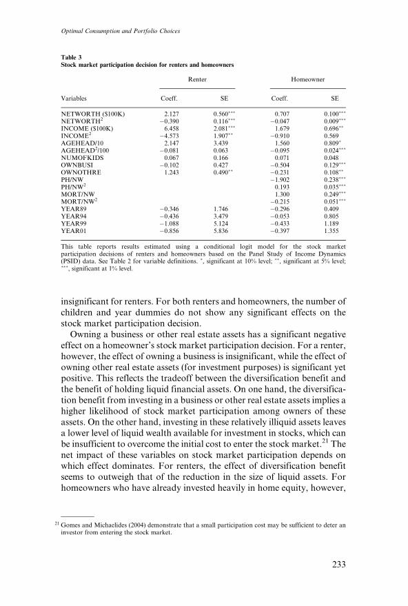
insignificant for renters. For both renters and homeowners, the number of

children and year dummies do not show any significant effects on the

stock market participation decision.

Owning a business or other real estate assets has a significant negative

effect on a homeowner’s stock market participation decision. For a renter,

however, the effect of owning a business is insignificant, while the effect of

owning other real estate assets (for investment purposes) is significant yetpositive. This reflects the tradeoff between the diversification benefit and

the benefit of holding liquid financial assets. On one hand, the diversifica-

tion benefit from investing in a business or other real estate assets implies a

higher likelihood of stock market participation among owners of these

assets. On the other hand, investing in these relatively illiquid assets leaves

a lower level of liquid wealth available for investment in stocks, which can

be insufficient to overcome the initial cost to enter the stock market.21 The

net impact of these variables on stock market participation depends onwhich effect dominates. For renters, the effect of diversification benefit

seems to outweigh that of the reduction in the size of liquid assets. For

homeowners who have already invested heavily in home equity, however,

Table 3Stock market participation decision for renters and homeowners

Renter Homeowner

Variables Coeff. SE Coeff. SE

NETWORTH ($100K) 2.127 0.560�� 0.707 0.100��

NETWORTH2 �0.390 0.116�� 0.047 0.009��

INCOME ($100K) 6.458 2.081�� 1.679 0.696��

INCOME2 �4.573 1.907�� 0.910 0.569AGEHEAD/10 2.147 3.439 1.560 0.809�

AGEHEAD2/100 �0.081 0.063 �0.095 0.024��

NUMOFKIDS 0.067 0.166 0.071 0.048OWNBUSI �0.102 0.427 �0.504 0.129��

OWNOTHRE 1.243 0.490�� 0.231 0.108��

PH/NW �1.902 0.238��

PH/NW2 0.193 0.035��

MORT/NW 1.300 0.249��

MORT/NW2 �0.215 0.051��

YEAR89 �0.346 1.746 �0.296 0.409YEAR94 �0.436 3.479 �0.053 0.805YEAR99 �1.088 5.124 �0.433 1.189YEAR01 �0.856 5.836 �0.397 1.355

This table reports results estimated using a conditional logit model for the stock marketparticipation decisions of renters and homeowners based on the Panel Study of Income Dynamics(PSID) data. See Table 2 for variable definitions. �, significant at 10% level; ��, significant at 5% level;��, significant at 1% level.

21 Gomes and Michaelides (2004) demonstrate that a small participation cost may be sufficient to deter aninvestor from entering the stock market.


233

owning a business or other real estate assets reduces the total available

liquid funds to such a low level that they find it inefficient to invest

in stocks.

All housing-related variables have a significant impact on homeowners’

stock market participation decisions. Specifically, the home-value–net-worth ratio affects stock market participation negatively but at a

decreasing rate.22 This is consistent with the participation cost

explanation: A higher home-value–net-worth ratio implies less liquid

wealth is available for equity investments. Interestingly, the outstanding

mortgage–net-worth ratio has a positive effect on homeowners’ stock

market participation decisions. This can be attributed to the effects of

house liquidation cost and refinancing charges. Consider two households

with identical house values and identical levels of net worth but differentoutstanding mortgage balances. The household with a higher mortgage–

net-worth ratio holds more wealth in liquid form and less in illiquid home

equity. In the event of a large negative shock to stock returns, the house-

hold with more wealth in liquid form can better weather the shock without

having to incur refinancing charges or selling costs to access home equity.

For homeowners, a high net-worth–income ratio is associated with

higher equity proportions in both their net worth and liquid financial

assets (Table 4). Recall that our model predicts that the homeowner’sequity proportions are hump-shaped in the net-worth–income ratio. Our

empirical results suggest that most homeowners lie on the upward sloping

segment of the equity proportion and net-worth–income ratio relation-

ship. The effect of the net-worth–income ratio is, however, insignificant

for renters. Income has no significant effect on either renters’ or home-

owners’ equity proportions in either net worth or liquid financial assets.

This is consistent with the specification in our theoretical model and

suggests that level variables such as net worth and income affectasset allocations mostly through the market participation decision.

Both equity proportion measures increase significantly as a renter ages.

While a homeowner’s net worth equity proportion is hump-shaped in age,

his liquid financial assets equity proportion decreases in age. While these

results are largely consistent with our findings based on state space and

simulation analysis, there are also some notable differences. Empirically,

investors (particularly renters and young homeowners) seem to stay

within the upward-sloping portion of the age–equity proportion relationfor an extended period of time, that is, their equity proportions peak much

later. For instance, based on our estimation, the net worth equity propor-

tion reaches its peak value at age 43.3 for homeowners. This suggests that

22 The estimated coefficients imply that the impact reaches a minimum at the house-value–net-worth ratioof 4.9, implying that the vast majority of households are on the declining portion of the quadratic curve.


234

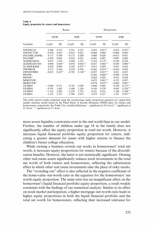
more severe liquidity constraints exist in the real world than in our model.

Further, the number of children under age 18 in the family does not

significantly affect the equity proportion in total net worth. However, it

increases liquid financial portfolio equity proportion for renters, indi-

cating a greater demand for assets with higher returns to finance thechildren’s future college education.

While owning a business crowds out stocks in homeowners’ total net

worth, it increases equity proportions for renters because of the diversifi-

cation benefits. However, the latter is not statistically significant. Owning

other real estate assets significantly reduces stock investments in the total

net worth of both renters and homeowners, reflecting the substitution

effect in which other real estate investments take the place of risky stocks.

The ‘‘crowding out’’ effect is also reflected in the negative coefficient ofthe home-value–net-worth ratio in the equation for the homeowners’ net

worth equity proportion. The same ratio has an insignificant effect on the

homeowner’s liquid financial portfolio equity proportion, a result weakly

consistent with the findings of our numerical analysis. Similar to its effect

on stock market participation, a higher mortgage–net-worth ratio leads to

higher equity proportions in both the liquid financial portfolio and the

total net worth for homeowners, reflecting their increased tolerance for

Table 4Equity proportion for renters and homeowners

Renter Homeowner

S/NW S/SB S/NW S/SB

Variables Coeff. SE Coeff. SE Coeff. SE Coeff. SE

NW/INC/10 0.268 0.315 0.231 0.231 0.035 0.017�� 0.055 0.027��

NW/INC2/100 �0.034 0.033 �0.025 0.023 �0.004 0.002� �0.006 0.003�

INCOME ($100K) 0.171 0.396 �0.172 0.280 0.008 0.020 �0.013 0.031INCOME2 �0.070 0.062 �0.010 0.052 �0.001 0.001 0.001 0.002AGEHEAD/10 0.073 1.614 0.994 1.237 0.234 0.133� �0.190 0.230AGEHEAD2/100 0.094 0.045�� 0.076 0.026�� 0.027 0.004�� 0.039 0.006��

NUMOFKIDS 0.078 0.069 0.182 0.071�� 0.013 0.009 0.023 0.016OWNBUSI 0.137 0.164 0.150 0.196 �0.062 0.019�� 0.034 0.028OWNOTHRE �0.651 0.247�� 0.702 0.148�� 0.037 0.013�� 0.031 0.023PH/NW �0.426 0.060�� 0.090 0.104PH/NW2 0.024 0.022 0.025 0.034MORT/NW 0.472 0.061�� 0.155 0.097MORT/NW2 �0.074 0.033�� 0.094 0.047��

YEAR89 �0.504 0.711 �0.791 0.589 0.044 0.065 0.320 0.115��

YEAR94 �0.701 1.443 �1.468 1.184 0.169 0.129 0.805 0.230��

YEAR99 �1.152 2.083 �2.259 1.791 0.251 0.191 1.180 0.340��

YEAR01 �1.151 2.357 �2.506 2.033 0.279 0.217 1.321 0.387��

This table reports results estimated using the second-stage equity proportion equation of a panel datasample selection model based on the Panel Study of Income Dynamics (PSID) data, for renters andhomeowners, respectively. See Table 2 for variable definitions. �, significant at 10% level; ��, significant at5% level; ��, significant at 1% level.


235

stock market shocks when a larger fraction of their wealth is in

liquid form.

Finally, while year dummies have positive but insignificant effects

on homeowners’ and renters’ net worth equity proportions, the equity

proportion in the homeowners’ liquid financial portfolio has, on average,increased significantly over time. The increase coincides with the relatively

strong performance of the stock markets over the sample time period.

This result points to the need to include portfolio rebalancing costs

and/or time-varying expected returns in order to match the model to

the empirically observed equity proportions in households’ liquid

portfolios.

4. Conclusion

In this article, we analyzed the optimal dynamic consumption, housing,and portfolio decisions for an investor who receives stochastic labor

income and also faces substantial housing risk, collateral requirements,

and liquidation cost. Our results indicate that the investor optimally

chooses to rent housing services when he faces severe liquidity constraints

and/or a high mortality rate. However, when the liquidity constraint is

relaxed the investor chooses owning a house over renting to benefit from

home ownership.

Home ownership has a significant impact on the investor’s portfoliodecision. When indifferent between renting and owning a house, the

investor who owns a house substitutes home equity for risky stocks in

his net worth, yet increases the equity proportion in his liquid financial

portfolio to take advantage of the diversification benefit afforded by the

low correlation between stock returns and housing returns. Following the

suboptimal policy of either always renting housing services or only own-

ing a house can lead to large welfare losses and drastically alter the

investor’s portfolio choices. Liquidation cost creates a no-adjustmentregion for housing services, which in turn influences the investor’s portfo-

lio decisions. When close to the boundaries of the no-adjustment region,

the investor holds a higher equity proportion in his liquid portfolio in

order to achieve the optimal risk-return tradeoff.

Detailed empirical analysis of households’ portfolio choices with risky

housing assets using the PSID data shows that renters and homeowners’

portfolio choices have different determinants and react differently to key

variables such as the net-worth–income ratio and investor age. Thisempirical evidence lends some support to the predictions of our model

based on both policy rules and the simulation analysis. Possible future

extensions include incorporating refinancing costs, as in Campbell and

Cocco (2003), and endogenizing the cost differential between renting and

owning on the basis of moral hazard and/or adverse selection.


236

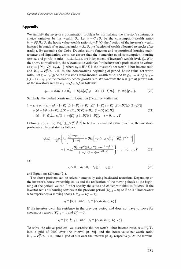
Appendix

We simplify the investor’s optimization problem by normalizing the investor’s continuous

choice variables by his wealth Qt. Let ct¼Ct =Qt be the consumption–wealth ratio;

ht ¼ PHt Ht=Qt the house value–wealth ratio; bt¼Bt=Qt the fraction of the investor’s wealth

invested in bonds after trading; and st¼St=Qt the fraction of wealth allocated to stocks after

trading. By assuming the Cobb–Douglas utility function and proportional housing main-

tenance and liquidation costs, we ensure that the numeraire good consumption, housing

service, and portfolio rules, {ct, ht, bt, st}, are independent of investor’s wealth level,Qt. With

the above normalization, the relevant state variables for the investor’s problem can be written

as xt ¼ fDot�1,D

mt ,wt, �hht�1g, where wt¼Wt=Yt is the investor’s net-worth–labor-income ratio

and �hht�1 ¼ PHt Ht�1=Wt is the homeowner’s beginning-of-period house-value–net-worth

ratio. Let yt¼Yt /Qt be the investor’s labor-income–wealth ratio, and let ~ggtþ1 ¼ D logYtþ1 ¼f ðtþ 1Þ þ etþ1 be the real labor-income growth rate.We can write the real (gross) growth rate

of the investor’s wealth qtþ1¼Qtþ1=Qt as follows:

qtþ1 ¼ btRf þ stR~S

tþ1 þDot ht½R

~H

tþ1ð1�fÞ�ð1�dÞRf � þ yt expf~ggtþ1g: ð20Þ

Similarly, the budget constraint in Equation (7) can be written as:

1 ¼ ct þ bt þ st þ aht½ð1�Dot�1Þð1�Do

t Þ þDot�1D

mt ð1�Do

t Þ þDot�1ð1�Dm

t ÞDstð1�Do

t Þ�þ ðcþ dÞht½ð1�Do

t�1ÞDot þDo

t�1Dm0 D

ot þDo

t�1ð1�Dm0 ÞDs

tDot � ð21Þ

þ ðcþ d�fÞ�hht�1w=ð1þ wÞ½Dot�1ð1�Dm

t Þð1�DstÞ�, t ¼ 0, . . . ,T

Defining vtðxtÞ ¼ VtðXtÞ=½ðQt=PHv

t Þ1�g � to be the normalized value function, the investor’s

problem can be restated as follows:

vtðxtÞ ¼ maxaðtÞ

ltðc1�v

t hvt Þ1�g

ð1�gÞ þ bEt vtþ1ðxtþ1Þqð1�gÞtþ1 ð~RRH

tþ1Þvðg�1Þ

h i" #(

þ ð1�ltÞbð1�bLÞ½ALv


ð1�bÞð1�gÞðaÞvð1�gÞ

), t ¼ 0; . . . ;T ð22Þ

s.t.

ct > 0, ht > 0, bt � 0, st � 0 ð23Þ

and Equations (20) and (21).

The above problem can be solved numerically using backward recursion. Depending on

the investor’s house ownership status and the realization of the moving shock at the begin-

ning of the period, we can further specify the state and choice variables as follows. If the

investor rents his housing services in the previous period (Dot�1 ¼ 0) or if he is a homeowner

who experiences a moving shock (Dot�1 ¼ Dm

t ¼ 1),

xt �fwtg and at �fct, ht, bt, st,Dot g:

If the investor owns his residence in the previous period and does not have to move for

exogenous reasons (Dot�1 ¼ 1 and Dm

t ¼ 0),

xt �fwt, �hht�1g and at �fct, ht, bt, st,Dot ,D

stg:

To solve the above problem, we discretize the net-worth–labor-income ratio, w¼Wt /Yt,

into a grid of 2000 over the interval [0, 50], and the house-value–net-worth ratio,�hht�1 ¼ PH

t Ht�1=Wt, into a grid of 500 over the interval [0, 4], respectively. At the terminal


237

date T, the investor’s value function takes the value of the bequest function and is

a constant:

vT ðxT Þ ¼bð1�bLÞ½ALv


ð1�bÞð1�gÞðaÞvð1�gÞ ð24Þ

at all points in the state space. The value function at date T is then used to solve for the

optimal decision rules for all points on the state space grid at date T� 1. Linear interpolation

is used to calculate the value function for points in the state space that lie between grid points.

The procedure is repeated recursively for each time period until the solution for date t¼ 0

is found.

ReferencesAnderson, R. N., 2001, ‘‘United State Life Tables 1998,’’ National Vital Statistics Reports, 48, 1–40.

Campbell, J., and J. F. Cocco, 2003, ‘‘Household Risk Management and Optimal Mortgage Choice,’’Quarterly Journal of Economics, 118, 1149–1194.

Carroll, C. D., and W. E. Dunn, 1997, ‘‘Unemployment Expectations, Jumping (S,s)Triggers, and Household Balance Sheets,’’ NBER Macroeconomics Annual, 165–229, MIT Press,Cambridge, MA.

Claus, J., and J. Thomas, 2001, ‘‘Equity Premia as Low as Three Percent? Evidence from Analysts’Earnings Forecasts for Domestic and International Stock Markets,’’ Journal of Finance 56, 1629–1666.

Cocco, J. F., 2004, ‘‘Portfolio Choice in the Presence of Housing,’’ Review of Financial Studies,forthcoming.

Cocco, J. F., F. J. Gomes, and P. J. Maenhout, 2004, ‘‘Consumption and Portfolio Choice over theLife-Cycle,’’ Review of Financial Studies, forthcoming.

Damgaard, A., B. Fuglsbjerg, and C. Munk, 2003, ‘‘Optimal Consumption and Investment Strategieswith a Perishable and an Indivisible Durable Consumption Good,’’ Journal of Economic Dynamics andControl, 28, 209–253.

Dammon, R. M., C. S. Spatt, and H. H. Zhang, 2001, ‘‘Optimal Consumption and Investment withCapital Gains Taxes,’’ Review of Financial Studies, 14, 583–616.

Davis, S. J., and P. Willen, 2000, ‘‘Occupation-Level Income Shocks and Asset Returns: TheirCovariance and Implications for Portfolio Choice,’’ working paper, Graduate School of Business,Univeristy of Chicago.

Deng, Y., J. M. Quigley, and R. Van Order, 2000, ‘‘Mortgage Terminations, Heterogeneity and theExercise of Mortgage Options,’’ Econometrica, 68, 275–308.

Fama, E. F., and K. R. French, 2002, ‘‘The Equity Premium,’’ Journal of Finance, 57, 637–659.

Flavin, M., and T. Yamashita, 2002, ‘‘Owner-Occupied Housing and the Composition of the HouseholdPortfolio over the Life Cycle,’’ American Economic Review, 92, 345–362.

Goetzmann, W. N., and M. Spiegel, 2000, ‘‘The Policy Implication of Portfolio Choice in UnderservedMortgage Markets,’’ working paper, Yale University.

Gomes, F., and A. Michaelides, 2004, ‘‘Optimal Life-Cycle Asset allocation: Understanding theEmpirical Evidence,’’ Journal of Finance, forthcoming.

Grossman, S. J., and G. Laroque, 1990, ‘‘Asset Pricing and Optimal Portfolio Choice in the Presence ofIlliquid Durable Consumption Goods,’’ Econometrica, 58, 25–51.

Heaton, J., and D. Lucas, 2000a, ‘‘Portfolio Choice and Asset Prices: The Importance of EntrepreneurialRisk’’, Journal of Finance, 55, 1163–1198.


238

Heaton, J., and D. Lucas, 2000b, ‘‘Portfolio Choice in the Presence of Background Risk’’, EconomicJournal, 110, 1–26.

Hu, X., 2002, ‘‘Portfolio Choice for Homeowners,’’ working paper, Northwestern University.

Jagannathan, R., and N. R. Kocherlakota, 1996, ‘‘Why Should Older People Invest Less in Stocks ThanYounger People?’’ Federal Reserve Bank of Minneapolis Quarterly Review, 20, 11–23.

Kullmann, C., and S. Siegel, 2003, ‘‘Real Estate and its Role in Household Portfolio Choice,’’ workingpaper, University of British Columbia.

Kyriazidou, E., 1997, ‘‘Estimation of a Panel Data Sample Selection Model,’’ Econometrica, 65,1335–1364.

Powell, J. L., 1994, ‘‘Estimation of Semiparametric Models,’’ Handbook of Econometrics, 4, 2444–2521.

U.S. Department of Labor, Bureau of Labor Statistics, 2003, Consumer Expenditures in 2001,Report 966.

U.S. Census Bureau, Population Division, 2003, Geographic Mobility: March 2000–March 2001.

U.S. Census Bureau, Housing and Household Economic Statistics Division, 1992, 1991 ResidentialFinance Survey.

Viceira, L. M., 2001, ‘‘Optimal Portfolio Choice for Long-Horizon Investors with Nontradable LaborIncome,’’ Journal of Finance, 56, 433–470.

Vissing-Jogensen, A., 2002, ‘‘Towards an Explanation of Household Portfolio Heterogeneity:Nonfinancial Income and Participation Cost Structures,’’ working paper, University of Chicago.

Yao, R., and H. H. Zhang, 2004, ‘‘Optimal Life-Cycle Asset allocation with Housing as a Collateral,’’working paper, Baruch College and University of North Carolina.


239

Documents

Optimal Consumption and Portfolio Choices with …hxz054000/RFS_YaoZhang.pdfOptimal Consumption and Portfolio Choices with Risky Housing and Borrowing Constraints Rui Yao Baruch College,