Optimal and System Myopic Policies for Multi-Echelon

Optimal and System Myopic Policies for Multi-Echelon Production/Inventory AssemblySystemsAuthor(s): Leroy B. Schwarz and Linus SchrageSource: Management Science, Vol. 21, No. 11, Theory Series (Jul., 1975), pp. 1285-1294Published by: INFORMSStable URL: http://www.jstor.org/stable/2629890 .Accessed: 20/05/2011 12:18

Your use of the JSTOR archive indicates your acceptance of JSTOR's Terms and Conditions of Use, available at .http://www.jstor.org/page/info/about/policies/terms.jsp. JSTOR's Terms and Conditions of Use provides, in part, that unlessyou have obtained prior permission, you may not download an entire issue of a journal or multiple copies of articles, and youmay use content in the JSTOR archive only for your personal, non-commercial use.

Please contact the publisher regarding any further use of this work. Publisher contact information may be obtained at .http://www.jstor.org/action/showPublisher?publisherCode=informs. .

Each copy of any part of a JSTOR transmission must contain the same copyright notice that appears on the screen or printedpage of such transmission.

JSTOR is a not-for-profit service that helps scholars, researchers, and students discover, use, and build upon a wide range ofcontent in a trusted digital archive. We use information technology and tools to increase productivity and facilitate new formsof scholarship. For more information about JSTOR, please contact [email protected].

INFORMS is collaborating with JSTOR to digitize, preserve and extend access to Management Science.

http://www.jstor.org

http://www.jstor.org/action/showPublisher?publisherCode=informs

http://www.jstor.org/stable/2629890?origin=JSTOR-pdf

http://www.jstor.org/page/info/about/policies/terms.jsp

http://www.jstor.org/action/showPublisher?publisherCode=informs

MANAGEMENT SCIENCE Vol. 21, No. 11, July 197

Printed in U.S.A.

OPTIMAL AND SYSTEM MYOPIC POLICIES FOR MULTI-ECHELON PRODUCTION/INVENTORY

ASSEMBLY SYSTEMS*

LEROY B. SCHWARZt AND LINUS SCHRAGE? ?

In this paper optimal and near optimal policies are proposed for multi-echelon production/inventory assembly systems under continuous review with constant demand over an infinite planning horizon. Costs at each stage consist of a fixed charge per order or production setup plus a linear holding cost on "echelon" inventory. The objective is minimization of average cost per unit time.

The major results of this paper are: a mathematically simple, often optimal, "system myopic" solution, a lower bound on the closeness to optimality of this solution, and a branch and bound algorithm which usually finds the optimal solution quickly.

1. Introduction

In this paper we describe optimal and near optimal policies for operating single product multi-echelon assembly production/inventory systems. In a multi-echelon assembly system each stage (which may be a production site, an assembly site, or merely a stocking site) obtains input from one or more immediate predecessors, perhaps with some delivery lag, and supplies output to a single successor, again with a possible delivery lag. The final stage, stage 1, satisfies the customer demand.

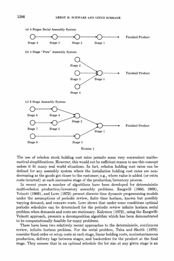
Figure 1 shows three possible configurations of assembly systems, including (a) the serial system, in which each stage has only one predecessor stage; and (b) the pure assembly system, in which stages 2, 3, . . . , N are immediate predecessors of stage 1. Examples of assembly systems abound in the real world; e.g., the manufacture and assembly of automobiles, electrical appliances, etc. Serial systems are frequently found in processing industries; e.g., the steel or aluminum industries where the stages represent different physical and/or chemical transformations of the same basic material (ore, pig iron, sheet steel, etc.). Clark (1972) has an extensive survey of multi-echelon models.

Our objective is to select ordering policies for assembly systems which minimize (or nearly minimize) average system cost per unit time over an infinite planning horizon when the customer demand rate is constant. Costs are of two types: a setup or order cost incurred at each stage whenever a batch is ordered or produced at that stage, and a holding cost for each stage charged continuously over time which is linear in the so-called "echelon" inventory at that stage.

Clark and Scarf (1960) define the echelon stock of stage j as the number of units in the system which are in or have passed through stage j but have as yet not been sold.

* Processed by Professor Edward J. Ignall, Departmental Editor for Dynamic Programming and Inventory Theory; received July 1973, revised April 1974 and October 1974. This paper has been with the authors 6 months for revision.

t University of Rochester. ? University of California, Los Angeles. ? The authors wish to acknowledge the valuable comments of Jack Williams on an earlier draft of

this paper. 1285

Copyright (D 1975, The Institute of Management Sciences

1286 LEROY B. SCHWARZ AND LINUS SCHRAGE

(a) 4 Stages Serial Assembly System

Finished Product

Stage 4 Stage 3 Stage 2 Stage 1

(b) 4 Stage "Pure" Assembly System

Stalge2\

0 - Finished Product

Stage 3 Stage 1

Stage 4

(c) 8 Stage Assembly System

Stage 6 Stage 4

Finished Product Stage 7 Stage 55

Stage 8 Stage 3

FIGURE 1

The use of echelon stock holding cost rates permits some very convenient mathe- matical simplifications. However, this would not be sufficient reason to use this concept unless it fit many real world situations. In fact, echelon holding cost rates can be defined for any assembly system where the installation holding cost rates are nondecreasing as the goods get closer to the customer; e.g., where value is added (or extra costs incurred) at each successive stage of the production/inventory process.

In recent years a number of algorithms have been developed for deterministic multi-echelon production/inventory assembly problems. Zangwill (1966, 1969), Veinott (1969), and Love (1972) present discrete time dynamic programming models under the assumptions of periodic review, finite time horizon, known but possibly varying demand, and concave costs. Love shows that under some conditions optimal periodic schedules can be determined for the periodic review infinite horizon serial problem when demands and costs are stationary. Kalymon (1972), using the Zangwill- Veinott approach, presents a decomposition algorithm which has been demonstrated to be computationally feasible for many problems.

There have been two relatively recent approaches to the deterministic, continuous review, infinite horizon problem. For the serial problem, Taha and Skeith (1970) consider fixed order or setup costs at each stage, linear holding costs, noninstantaneous production, delivery lags between stages, and backorders for the product at the final stage. They assume that in an optimal schedule the lot size at any given stage is an

POLICIES FOR MULTI-ECHELON PRODUCTION/INVENTORY SYSTEMS 1287

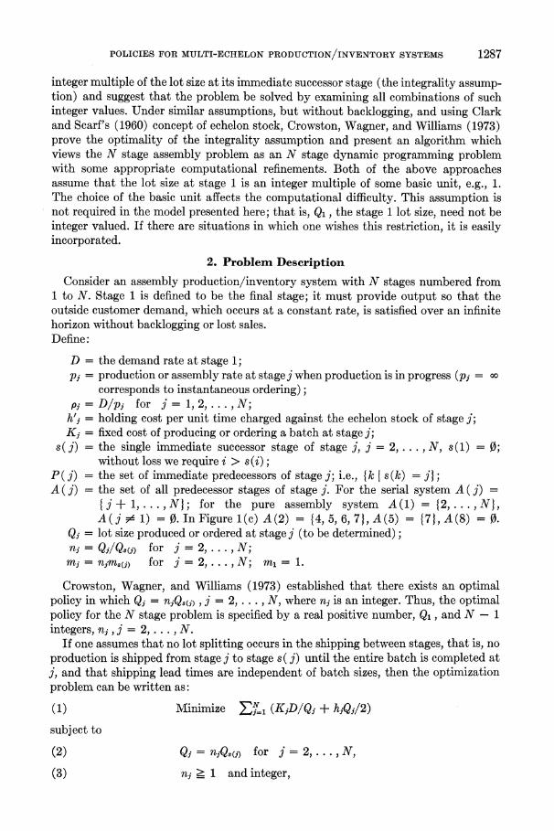
integer multiple of the lot size at its immediate successor stage (the integrality assumption) and suggest that the problem be solved by examining all combinations of such integer values. Under similar assumptions, but without backlogging, and using Clark and Scarf's (1960) concept of echelon stock, Crowston, Wagner, and Williams (1973) prove the optimality of the integrality assumption and present an algorithm which views the N stage assembly problem as an N stage dynamic programming problem with some appropriate computational refinements. Both of the above approaches assume that the lot size at stage 1 is an integer multiple of some basic unit, e.g., 1. The choice of the basic unit affects the computational difficulty. This assumption is not required in the model presented here; that is, Qi, the stage 1 lot size, need not be integer valued. If there are situations in which one wishes this restriction, it is easily incorporated.

2. Problem Description

Consider an assembly production/inventory system with N stages numbered from 1 to N. Stage 1 is defined to be the final stage; it must provide output so that the outside customer demand, which occurs at a constant rate, is satisfied over an infinite horizon without backlogging or lost sales. Define:

D = the demand rate at stage 1; pj = production or assembly rate at stage j when production is in progress (pj = 0o

corresponds to instantaneous ordering); pj = D/pj for j = 1, 2, . . ., N;

h'j = holding cost per unit time charged against the echelon stock of stage j; Kj = fixed cost of producing or ordering a batch at stage j;

s( j) = the single immediate successor stage of stage j, j = 2, ... , N, s(1) = 0; without loss we require i > s(i);

P( j) = the set of immediate predecessors of stage j; i.e., {k I s(k) = j}; A ( j) = the set of all predecessor stages of stage j. For the serial system A ( j) =

{j+ 1,... ,N}; for the pure assembly system A(1) = {2,... .7N)) A( j # 1) = 0. In Figure l(c) A(2) = {4, 5, 6, 7}, A(5) = {7}, A(8) = 0.

Qj = lot size produced or ordered at stage j (to be determined); nj = Qj/Qj(j) for j = 2, * N; mj = njm,(j) for j = 2, ...,N; m1 = 1.

Crowston, Wagner, and Williams (1973) established that there exists an optimal policy in which Qj = njQ8(j) , j = 2, . .. , N, where nj is an integer. Thus, the optimal policy for the N stage problem is specified by a real positive number, Qi, and N - 1 integers, nj , j = 2, ... , N.

If one assumes that no lot splitting occurs in the shipping between stages, that is, no production is shipped from stage j to stage s ( j) until the entire batch is completed at j, and that shipping lead times are independent of batch sizes, then the optimization problem can be written as:

(1) Minimize N (KjD/Qj + hjQjl2)

subject to

(2) Qj =njQ(j) for j = 2, . . . ,N,

(3) nj 1 and integer,


where

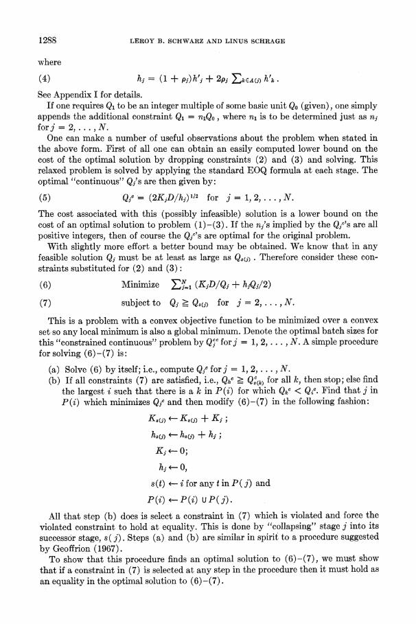
(4) hj = (1 + p,)h'j + 2Pi EkEA(&) h'k.

See Appendix I for details. If one requires Q, to be an integer multiple of some basic unit Qo (given), one simply

appends the additional constraint Q- = n,Qo, where ni is to be determined just as n1 for] = 2 . .. . N.

One can make a number of useful observations about the problem when stated in the above form. First of all one can obtain an easily computed lower bound on the cost of the optimal solution by dropping constraints (2) and (3) and solving. This relaxed problem is solved by applying the standard EOQ formula at each stage. The optimal "continuous" Qj's are then given by:

(5) Qi'_(2KjD/h)"12 for j = 1, 2, . .. , N.

The cost associated with this (possibly infeasible) solution is a lower bound on the cost of an optimal solution to problem (1) -(3). If the nj's implied by the Qjc's are all positive integers, then of course the Qjc's are optimal for the original problem.

With slightly more effort a better bound may be obtained. We know that in any feasible solution Qj must be at least as large as Q,j) . Therefore consider these constraints substituted for (2) and (3):

(6) Minimize E (K1D/Q1 + hjQ1l2)

(7) subject to Qj > Q,(j) for j = 2, . . . , N.

This is a problem with a convex objective function to be minimized over a convex set so any local minimum is also a global minimum. Denote the optimal batch sizes for this "constrained continuous" problem by Q'` for ] = 1, 2, ... , N. A simple procedure for solving (6) -(7) is:

(a) Solve (6) by itself; i.e., compute Qjc for j = 1, 2, . . . ,N. (b) If all constraints (7) are satisfied, i.e., Qkc > Q:(k) for all k, then stop; else find

the largest i such that there is a k in P (i) for which Qkc < Qic. Find that j in P(i) which minimizes QjC and then modify (6)-(7) in the following fashion:

K8(j) , K8(j) + Ki ;

h*()- h8(i) + hi ;

Kj -- 0;

h- 0,

s(t) -i for any t in P(j) and

P( -P(i) UP(j).

All that step (b) does is select a constraint in (7) which is violated and force the violated constraint to hold at equality. This is done by "collapsing" stage j into its successor stage, s (j). Steps (a) and (b) are similar in spirit to a procedure suggested by Geoffrion (1967).

To show that this procedure finds an optimal solution to (6)-(7), we must show that if a constraint in (7) is selected at any step in the procedure then it must hold as an equality in the optimal solution to (6)-(7).


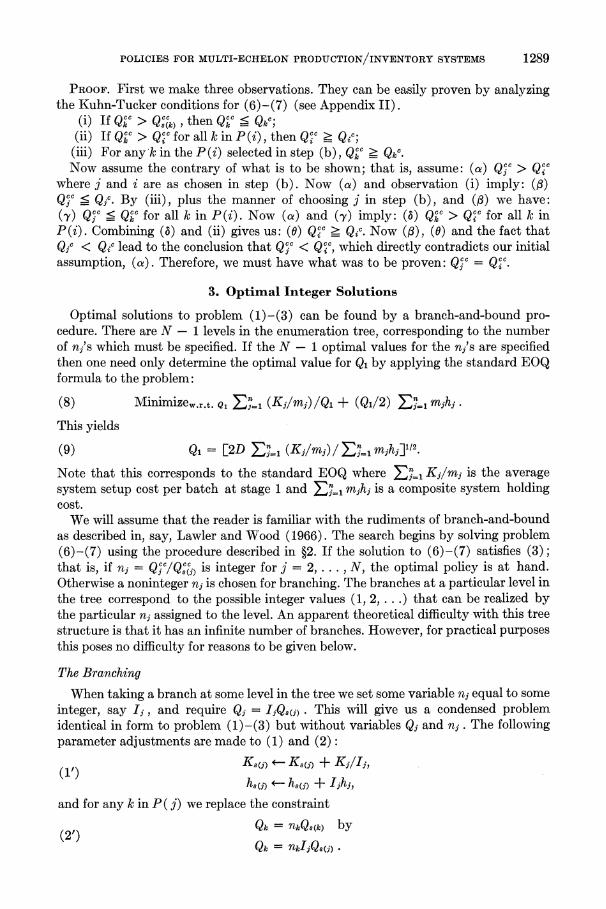
PROOF. First we make three observations. They can be easily proven by analyzing the Kuhn-Tucker conditions for (6)-(7) (see Appendix II).

(i) If QZk > Q&C) , then Q"' _ Qkc;

(ii) If Q C > Q. for all k in P(i), then Q. > Q (iii) For any'k in the P(i) selected in step (b), Q > Qkc.

Now assume the contrary of what is to be shown; that is, assume: (a) QjC > QT' where j and i are as chosen in step (b). Now (a) and observation (i) imply: (,B) QjC _ QjC. By (iii), plus the manner of choosing j in step (b), and (A) we have: (y) QjC < Q"" for all k in P(i). Now (a) and (y) imply: (a) Q"" > QT for all k in P(i). Combining (a) and (ii) gives us: (0) QT> > QiC. Now (A), (0) and the fact that QjC < Q.C lead to the conclusion that Qj < QC, which directly contradicts our initial assumption, (a). Therefore, we must have what was to be proven: QjC = Q$C.

3. Optimal Integer Solutions

Optimal solutions to problem (1)-(3) can be found by a branch-and-bound procedure. There are N - 1 levels in the enumeration tree, corresponding to the number of nj's which must be specified. If the N - 1 optimal values for the nj's are specified then one need only determine the optimal value for Qi by applying the standard EOQ formula to the problem:

(8) Minimizew.r.t. Q, Z,=1 (Kj/mj)/Qi + (Q1/2) 2j-1 m3h1.

This yields

(9) Qi = [2D EZ8_1 (Kj/mj) / mihi]1.

Note that this corresponds to the standard EOQ where _ Kj/mj is the average system setup cost per batch at stage 1 and EJ=2 mjhj is a composite system holding cost.

We will assume that the reader is familiar with the rudiments of branch-and-bound as described in, say, Lawler and Wood (1966). The search begins by solving problem (6)-(7) using the procedure described in ?2. If the solution to (6)-(7) satisfies (3); that is, if ni = Qjc/Q() is integer for j = 2, . . . , N, the optimal policy is at hand. Otherwise a noninteger nj is chosen for branching. The branches at a particular level in the tree correspond to the possible integer values (1, 2, . . .) that can be realized by the particular nj assigned to the level. An apparent theoretical difficulty with this tree structure is that it has an infinite number of branches. However, for practical purposes this poses no difficulty for reasons to be given below.

The Branching

When taking a branch at some level in the tree we set some variable nj equal to some integer, say Ij, and require Qj = IjQs(j). This will give us a condensed problem identical in form to problem (1)-(3) but without variables Qj and nj . The following parameter adjustments are made to (1) and (2):

.Ks(j) - Ks(j) + Ki/Ij,

ks(i) <- s(i) + Ijhj, and for any k in P ( j) we replace the constraint

(2') Qk = nkQs(k) by Qk = nklQ(J)


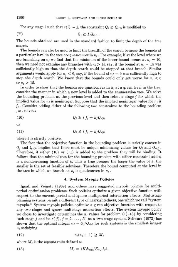
For any stage i such that s(i) = j, the constraint Qi > Q,i is modified to

(V) ~~~~~~~~Qi >_ IjQs(j)

The bounds obtained are used in the standard fashion to limit the depth of the tree search.

The bounds can also be used to limit the breadth of the search because the bounds at a particular level in the tree are quasiconvex in nj . For example, if at the level where we are branching on nj we find that the minimum of the lower bound occurs at nj = 10, then we need not examine any branches withnj > 15, say, if the bound at nj = 15 was sufficiently high so that the depth search could be stopped at that branch. Similar arguments would apply for nj < 6, say, if the bound at nj = 6 was sufficiently high to stop the depth search. We know that the bounds could only get worse for nj < 6 or nj> 15.

In order to show that the bounds are quasiconvex in nj at a given level in the tree, consider the manner in which a new level is added to the enumeration tree. We solve the bounding problem at the previous level and then select a stage j for which the implied value for nj is noninteger. Suppose that the implied noninteger value for nj is fj. Consider adding either of the following two constraints to the bounding problem just solved:

(10) Qj _ fj + k) Qj

or

(11) Qj (fj -k)Q

where k is strictly positive. The fact that the objective function in the bounding problem is strictly convex in

Qj and Q8fj) implies that there must be unique minimizing values for Qj and Q.(j) . Therefore, if either (10) or (11) is added to the problem they will be binding. It follows that the minimal cost for the bounding problem with either constraint added is a nondecreasing function of k. This is true because the larger the value of k, the smaller is the set of feasible solutions. Therefore the bound computed at the level in the tree in which we branch on nj is quasiconvex in nj .

4. System Myopic Policies

Ignall and Veinott (1969) and others have suggested myopic policies for multiperiod optimization problems. Such policies optimize a given objective function with respect to the current period and ignore multiperiod interaction effects. Multistage planning systems permit a different type of nearsightedness, one which we call "system myopia." System myopic policies optimize a given objective function with respect to any two stages and ignore multistage interaction effects. The system myopic policy we chose to investigate determines the ni values for problem (1)-(3) by considering each stage j and its s( j), j = 2, . . . , N, as a two-stage system. Schwarz (1973) has shown that the optimal integer nj = Qj/Qs(j) for such systems is the smallest integer nj satisfying

(12) nj(ni + 1) > M1

where Mj is the myopia ratio defined as

(13) Mj = (Kjh,(j)/K,(j)hj).


We shall denote these n values njm,j = 2,... , N. After the njm are computed, Qi is computed using (9).

There is much to recommend the application of system myopic policies. First, the system myopic policy is trivially easy to determine when compared to the algorithm for determining the optimal nj's. Second, the cost of the system myopic policy may be quite close to the cost of the optimal policy. In order to see this, note that the njm represent one of the lattice points immediately surrounding the optimal solution to problem (1)-(2). That is, if we denote the set of optimal continuous nj's as njf =

Qjc/QC(j) = M'2, where the Qjc are defined as in (5), it is easily shown that lnjM - njc I < 1. Such proximity suggests that if we define C (nj) as the value of (1)

for given values of nj, j = 2, ... , N, and the correspondingly optimal Q, from (9), then C (njM) may be close to the value of C (njc), which is a lower bound on the value of C(nj*) where nj/ is the optimal nj, j = 2, . . . , N. Hence it follows that C(njM) may be close to C (nj*), j = 2, ... , N. Moreover, since it can be shown that (C(n3M) - C(njc))/C(njc) is in general a decreasing function of (njM -njc)/njc

one can argue that the larger the Mj, the closer C(njM) is to C(nj*). In other words, the larger the Mj's, the better the system myopic solution, all other things being equal.

Do we expect the Mj's to be large or small for problems with realistic parameters? If, as in many instances, the Kj's increase in j and the hj's decrease in j, we may expect the Mj's to be larger than one, how much larger depending on the increase (decrease) in the setup (holding) costs at higher stages of the system.

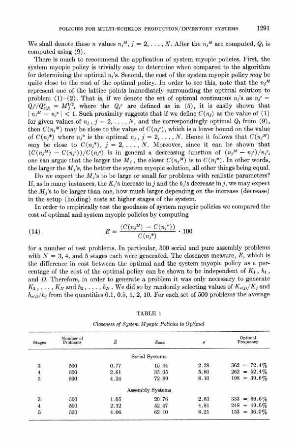
In order to empirically test the goodness of system myopic policies we compared the cost of optimal and system myopic policies by computing

(C (nim) - C (n.*)) 0 (14) E = C (nj*)

for a number of test problems. In particular, 500 serial and pure assembly problems with N = 3, 4, and 5 stages each were generated. The closeness measure, E, which is the difference in cost between the optimal and the system myopic policy as a per- centage of the cost of the optimal policy can be shown to be independent of K1, hi, and D. Therefore, in order to generate a problem it was only necessary to generate K2,. . . , KN and h2, . .. , hN . We did so by randomly selecting values of Ks(j)/Kj and hs(j)/hj from the quantities 0.1, 0.5, 1, 2, 10. For each set of 500 problems the average

TABLE 1

Closeness of System Myopic Policies to Optimal

Number of Optimal Stages Problems E Emax Frequency

Serial Systems

3 500 0.77 15.44 2.28 362 = 72.4% 4 500 2.61 35.05 5.80 262 = 52.4% 5 500 4.24 72.89 8.10 198 = 39.6%

Assembly Systems

3 500 1.05 20.76 2.63 333 = 66.6% 4 500 2.12 52.47 4.81 248 = 49.6% 5 500 4.06 62.10 8.21 153 = 36.0%


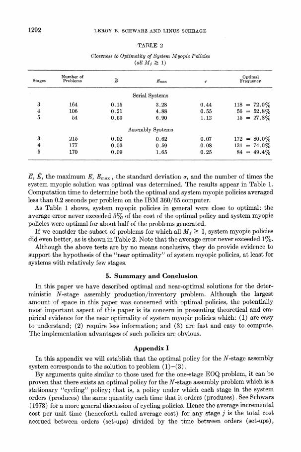
TABLE 2

Closeness to Optimality of System Myopic Policies (all Mj > 1)

Number of Optimal Stages Problems E Emax Frequency

Serial Systems

3 164 0.15 3.28 0.44 118 = 72.0% 4 106 0.21 4.88 0.55 56 = 52.8% 5 54 0.53 6.90 1.12 15 = 27.8%

Assembly Systems

3 215 0.02 0.62 0.07 172 = 80.0% 4 177 0.03 0.59 0.08 131 = 74.0% 5 170 0.09 1.65 0.25 84 = 49.4%

E, E, the maximum E, Emax, the standard deviation a-, and the number of times the system myopic solution was optimal was determined. The results appear in Table 1. Computation time to determine both the optimal and system myopic policies averaged less than 0.2 seconds per problem on the IBM 360/65 computer.

As Table 1 shows, system myopic policies in general were close to optimal: the average error never exceeded 5% of the cost of the optimal policy and system myopic policies were optimal for about half of the problems generated.

If we consider the subset of problems for which all Mj > 1, system myopic policies did even better, as is shown in Table 2. Note that the average error never exceeded 1%.

Although the above tests are by no means conclusive, they do provide evidence to support the hypothesis of the "near optimality" of system myopic policies, at least for systems with relatively few stages.

5. Summary and Conclusion

In this paper we have described optimal and near-optimal solutions for the deterministic N-stage assembly production/inventory problem. Although the largest amount of space in this paper was concerned with optimal policies, the potentially most important aspect of this paper is its concern in presenting theoretical and em- pirical evidence for the near optimality of system myopic policies which: (1) are easy to understand; (2) require less information; and (3) are fast and easy to compute. The implementation advantages of such policies are obvious.

Appendix I

In this appendix we will establish that the optimal policy for the N-stage assembly system corresponds to the solution to problem (1) -(3).

By arguments quite similar to those used for the one-stage EOQ problem, it can be proven that there exists an optimal policy for the N-stage assembly problem which is a stationary "cycling" policy; that is, a policy under which each stage in the system orders (produces) the same quantity each time that it orders (produces). See Schwarz (1973) for a more general discussion of cycling policies. Hence the average incremental cost per unit time (henceforth called average cost) for any stage j is the total cost accrued between orders (set-ups) divided by the time between orders (set-ups),


Qj/D. The average cost of the system is then simply the sum of the average costs for all stages.

For the N = 1 stage system, the development of the average cost is straightforward. A cycle begins when (Ql/pl) D = piQj units are on hand. This inventory is used to satisfy the outside demand during the time it takes to complete the production of Qi units, Ql/pl. When production begins, stage l's inventory increases at the rate (Pi - D), reaches a maximum of (1 - P1) Qi + piQ1, at which time production ceases, and declines at the rate D until the cycle ends with p'Qi units on hand Thus the average cost for a one-stage system is KiD/Q1 + h1Q1/2 where hi = (1 + pi) h'1.

Similarly, when there are no delivery lags a cycle for any stage in an N-stage system begins with an installation stock of pjQj and a corresponding echelon stock of P3Qj + EkES(j) PkQk , where S( j) is the set of all successors to stage j; that is, S ( j) = {s(j), s(s(j)), .. . , 1}. This stock grows at the rate (pj - D) until production ceases, at which time it declines at the rate D. Hence the average cost for stage j is KjD/Qj + h'j(pjQj + EkES(j) PkQk + (1 - pj)Qj/2).

Therefore the average cost for the N-stage system is

(15) 1n { KjD/Qj + h'j(1 - pj)Qj/2 + h'jpjQj + EkEs(j) h'jpkQk}.

After rearranging (15) and substituting (4) we obtain (1). Constraints (2) and (3) follow directly for the integrality assumption established by Crowston, et al.

The above development was based on the assumption that the delivery lag between stage j and s ( j), say lj, equals zero for all j = 2, . . ., N. However, fixed delivery lags have no incremental effect on costs because a given ij > 0 merely requires an additional average pipeline inventory between j and s( j) of ljD units, which increases average costs by the constant h'jljD.

Appendix II

Let us write the Kuhn-Tucker conditions associated with problem (6)-(7). Let Xk

be the Lagrange multiplier associated with the constraint Qk - Qs(k) for k = 2, 3, ... , N. The Q" 's, for k = 1, 2, ... , N, must satisfy the Kuhn-Tucker conditions:

(iv) -KkD/Qk2 + hk/2 - Xk + iEP(k) Xi = 0,

(v) Qk - Q8(k) 0,

(vi) Xk ? O,

(vii) Xk(Qk - Qs(k)) = 0.

The values Qkc are simply the values obtained for the Qk's in (iv) when we set all the X's = 0 and disregard (v).

First consider observation (i), namely, if QC > Qc) then Qc <? Qkc. Now Q'c > Qk implies by (vii) that Xk = 0. But EiEP(k) X > 0 in (iv) which implies that Q'C < Qkc.

Observation (ii) is: if Q'ci > Qkc for all i in P(k), then Q' > Qkc. Now Q7i > Q' for all i in P(k) implies by (vii) that Xi = 0 for all i in P(k). But -Xk < 0 in (iv), which implies that Qkc > Qkc.

Observation (iii) is that for any k in the P (i) selected in step (b) of the algorithm we must have Q" > Qk". Suppose Qkc < Qkc for some k in P (i) as selected in step (b) of the algorithm. Consider an alternative solution wherein Q" = Qkc and Q7c = QjC for all j E P(k). By construction and the selection of i in step (b), the alternative solution satisfies (7). Moreover, the alternative solution has a lower cost, so Q" < Qkc

cannot be true.


References

1. CLARK, A. J. AND SCARF, H., "Optimal Policies for a Multi-Echelon Inventory Problem," Management Science, 6 (July 1960), 475-490.

2. --, "An Informal Survey of Multi-Echelon Inventory Theory," Nav. Res. Log. Quart., 19 (Dec. 1972), 621-650.

3. CROWSTON, W. B., WAGNER, M. AND WILLIAMS, J. F., "Economic Lot Size Determination in Multi-Stage Assembly Systems," Management Science, 19 (January, 1973), 517-527.

4. GEOFFRION, A. M., "Reducing Concave Programs with Some Linear Constraints," SIAM J. Appl. Math., 15 (May 1967), 653-664.

5. IGNALL, E. J. AND VEINOTT, A. F. JR., "Optimality of Myopic Inventory Policies for Several Substitute Products," Management Science, 15 (January 1969), 284-304.

6. KALYMON, B. A., "A Decomposition Algorithm for Arborescence Inventory Systems," Operations Research, 20 (July-August 1972), 860-874.

7. LAWLER, E. L. AND WOOD, D. E., "Branch and Bound Methods: A Survey," Operations Research, 14 (July-August 1966), 699-719.

8. LOVE, S., "A Facilities in Series Inventory Model with Nested Schedules," Management Science, 18 (January 1972), 327-338.

9. SCHWARZ, L. B., "A Simple Continuous Review Deterministic One-Warehouse N-Retailer Inventory Problem," Management Science, 19 (January 1973), 555-566.

10. TAHA, H. A. AND SKEITH, R. W., "The Economic Lot Sizes in Multi-Stage Production Systems," AIIE Transactions, (June 1970), 157-162.

11. VEINOTT, A. F., JR., "Minimum Concave Cost Solution of Leontief Substitution Models of Multi-Facility Inventory Systems," Operations Research, 17 (March-April 1969), 262-291.

12. ZANGWILL, W. I., "A Deterministic Multi-Period Multi-Facility Production and Inventory Model," Operations Research, 14 (May-June 1966), 486-507.

13. --, "A Backlogging Model and a Multi-Echelon Model of a Dynamic Economic Lot Size Production System-A Network Approach," Management Science, 15 (May 1969), 506-527.

Documents

Optimal and System Myopic Policies for Multi-Echelon