Optimal Allocation with Costly Verification1

Elchanan Ben-Porath2 Eddie Dekel3 Barton L. Lipman4

First Preliminary DraftOctober 2011

Current DraftMarch 2013

1We thank Ricky Vohra, Benjy Weiss, and numerous seminar audiences for helpful com-ments. We also thank the National Science Foundation, grants SES–0820333 and SES-1227434(Dekel) and SES–0851590 (Lipman), and the US–Israel Binational Science Foundation (Ben-Porath and Lipman) for support for this research. Lipman also thanks Microsoft Research NewEngland for their hospitality while this draft was in progress and Alex Poterack for proofreading.

2Department of Economics and Center for Rationality, Hebrew University. Email: benpo-rat@math.huji.ac.il.

3Economics Department, Northwestern University, and School of Economics, Tel Aviv Uni-versity. Email: dekel@northwestern.edu.

4Department of Economics, Boston University. Email: blipman@bu.edu.

Abstract

A principal (dean) has an object (job slot) to allocate to one of I agents (departments).Each agent has a strictly positive value for receiving the object. Each agent also hasprivate information which determines the value to the principal of giving the object tohim. There are no monetary transfers but the principal can check the value associatedwith any individual at a cost which may vary across individuals. We characterize the classof optimal Bayesian mechanisms, that is, mechanisms which maximize the expected valueto the principal from his assignment of the good minus the costs of checking values. Oneparticularly simple mechanism in this class, which we call the favored–agent mechanism,specifies a threshold value v∗ and a favored agent i∗. If all agents other than i∗ reportvalues below v∗, then i∗ receives the good and no one is checked. Otherwise, whoeverreports the highest value is checked with probability 1 and receives the good iff her reportis confirmed. We show that all optimal mechanisms are essentially randomizations overoptimal favored–agent mechanisms.

1 Introduction

Consider the following environment: a principal has a good to allocate among a numberof agents, each of whom wants the good. Each agent i knows the value the principalreceives if he gives the good to i, but the principal does not. (This value need notcoincide with the value to i of getting the good.) The principal can verify the agents’private information at a cost, but cannot use transfers. There are a number of economicenvironments of interest that roughly correspond to this scenario; we discuss a few below.How does the principal maximize the expected gain from allocating the good less the costsof verification?

We characterize optimal mechanisms for such settings. We construct an optimalmechanism with a particularly simple structure which we call a favored–agent mechanism.There is a threshold value and a favored agent, say i. If each agent other than i reportsa value for the good below the threshold, then the good goes to the favored agent and noverification is required. If some agent other than i reports a value above the threshold,then the agent who reports the highest value is checked. This agent receives the good iffhis claims are verified and the good goes to any other agent otherwise.

In addition, we show that every optimal mechanism is essentially a randomizationover optimal favored–agent mechanisms. In this sense, we can characterize the full set ofoptimal mechanisms by focusing entirely on favored–agent mechanisms. By “essentially,”we mean that any optimal mechanism has the same outcomes as such a randomizationup to sets of measure zero.1 An immediate implication is that if there is a unique optimalfavored–agent mechanism, then there is essentially a unique optimal mechanism.

Finally, we give a variety of comparative statics. In particular, we show that an agentis more likely to be the favored agent the higher is the cost of verifying him, the “better”is his distribution of values in the sense of first order stochastic dominance (FOSD),and the less risky is his distribution of values in the sense of second order stochasticdominance (SOSD). We also show that the mechanism is, in a sense, almost a dominantstrategy mechanism and consequently is ex post incentive compatible.2

The standard mechanism–design approach to an allocation problem is to construct amechanism with monetary transfers and ignore the possibility of the principal verifyingthe agent’s information. In many cases obtaining information about the agent’s type ata cost is quite realistic (see examples below). Hence we think it is important to addthis option; this is the main goal of this paper. In our exploration of this option, we

1Two mechanisms have the same “outcome” if the interim probabilities of checking and allocatingthe good are the same; see Section 2 for details.

2More precisely, truthful reporting is an optimal strategy for agent i given any profile of reportingstrategies for the other agents.

1

take the opposite extreme position from the standard model and do not allow transfers.This obviously simplifies the problem, but we also find it reasonable to exclude transfers.Indeed, in many cases they are not used. In some situations, this may be becausetransfers have efficiency costs that are ignored in the standard approach. More specificallythe monetary resources each agent has might matter to the principal, so changing theallocation of monetary resources in order to allocate a good might be costly. In othersituations, the value to the principal of agent i getting the good may differ from the valueto agent i of getting the good, which reduces the usefulness of monetary transfers. Forexample, if the value to the principal of giving the good to i and the value to agent iof receiving it are independent, then, from the point of view of the principal, giving thegood to the agent who values it most is the same as random allocation. For these reasons,we adopt the opposite assumption to the standard one: we allow costly verification butdo not allow for transfers.

We now discuss some examples of the environment described above. Consider theproblem of the head of an organization — say, a dean — who has an indivisible resourceor good (say, a job slot) that can be allocated to any of several divisions (departments)within the organization (university). Naturally, the dean wishes to allocate this slotto that department which would fill the position in the way which best promotes theinterests of the university as a whole. Each department, on the other hand, would like tohire in its own department and puts less, perhaps no, value on hires in other departments.In addition, the department may well value candidates differently than the dean. Thedepartment, of course, has much more information regarding the candidates’ qualities andhence the value of the candidate to the dean. In such a situation, it is natural to assumethat the head of the organization can obtain information that can confirm whether thedepartment’s claims are correct. Obtaining and/or processing such information is costlyto the dean so this will also be taken into account.

Similar problems arise in areas other than organizational economics. For example,governments allocate various goods or subsidies which are intended not for those willingand able to pay the most but for those most in need. Hence allocation mechanisms basedon auctions or similar approaches cannot achieve the government’s goal, often leading tothe use of mechanisms which rely instead on some form of verification.3

As another example, consider the problem of choosing which of a set of job applicantsto hire for a job with a predetermined salary. Each applicant wants the job and presentsclaims about his qualifications for the job. The person in charge of hiring can verify theseclaims but doing so is costly.

3Banerjee, Hanna, and Mullainathan (2011) give the example of a government that wishes to allocatefree hospital beds. Their focus is the possibility that corruption may emerge in such mechanisms whereit becomes impossible for the government to entirely exclude willingness to pay from playing a role in theallocation. We do not consider such possibilities here. The matching literature also studies allocationproblems where transfers are considered inappropriate and hence are not used.

2

Literature review. Townsend (1979) initiated the literature on the principal–agent modelwith costly state verification. These models differ from what we consider in that theyinclude only one agent and allow monetary transfers. In this sense, one can see our workas extending the costly state verification framework to multiple agents when monetarytransfers are not possible. See also Gale and Hellwig (1985), Border and Sobel (1987),and Mookherjee and Png (1989). Our work is also related to Glazer and Rubinstein(2004, 2006), particularly the former which can be interpreted as model of a principaland one agent with limited but costless verification and no monetary transfers. Finally,it is related to the literature on mechanism design and implementation with evidence— see Green and Laffont (1986), Bull and Watson (2007), Deneckere and Severinov(2008), Ben-Porath and Lipman (2012), Kartik and Tercieux (2012), and Sher and Vohra(2011). With the exception of Sher and Vohra, these papers focus more on general issuesof mechanism design and implementation in these environments rather than on specificmechanisms and allocation problems. Sher and Vohra do consider a specific allocationquestion, but it is a bargaining problem between a seller and a buyer, very different fromwhat is considered here.

There is a somewhat less related literature on allocations without transfers but withcostly signals (McAfee and McMillan (1992), Hartline and Roughgarden (2008), Yoon(2011), Condorelli (2012), and Chakravarty and Kaplan (2013)).4 In these papers, agentscan waste resources to signal their values and the principal’s payoff is the value of thetype receiving the good less the cost of the wasted resources. The papers differ in theirassumptions about the cost, the number of goods to allocate, and so on, but the commonfeature is that wasting resources can be useful in allocating efficiently and that theprincipal may partially give up on allocative efficiency to save on these resources. See alsoAmbrus and Egorov (2012) who allow both monetary transfers and wasting of resourcesin a delegation model.

The remainder of the paper is organized as follows. In the next section, we presentthe model. Section 3 contains the characterization of the class of optimal mechanisms,showing all optimal mechanisms are essentially randomizations over optimal favored–agent mechanisms. Since these results show that we can restrict attention to favored–agent mechanisms, we turn in Section 4 to characterizing the set of best mechanisms inthis class. In Section 5, we give comparative statics and some examples. In Section 6,we sketch the proof of our uniqueness result and discuss several other issues. Section 7concludes. Proofs not contained in the text are in the Appendix.

4There is also a large literature on allocations without transfers, namely the matching literature; see,e.g., Roth and Sotomayor (1990) for a classic survey and Abdulkadiroglu and Sonmez (2013) for a morerecent one.

3

2 Model

The set of agents is I = {1, . . . , I}. There is a single indivisible good to allocate amongthem. The value to the principal of assigning the object to agent i depends on informationwhich is known only to i. Formally, the value to the principal of allocating the good toagent i is ti where ti is private information of agent i. The value to the principal ofassigning the object to no one is normalized to zero.5 We assume that the ti’s areindependently distributed. The distribution of ti has a strictly positive density fi overthe interval Ti ≡ [ti, ti] where 0 ≤ ti < ti < ∞. (All results extend to allowing thesupport to be unbounded above.) We use Fi to denote the corresponding distributionfunction. Let T =

∏i Ti.

The principal can check the type of agent i at a cost ci > 0. We interpret checkingas obtaining information (e.g., by requesting documentation, interviewing the agent, orhiring outside evaluators). If the principal checks some agent, she learns that agent’stype. The cost ci is interpreted as the direct cost to the principal of reviewing theinformation provided plus the costs to the principal associated with the resource cost tothe agent of being checked. The cost to the agent of providing information is assumedto be zero. To understand this, think of the agent’s resources as allocated to activitieswhich are either directly productive for the principal or which provide information forchecking claims. The agent is indifferent over how these resources are used since theywill all be used regardless. Thus by directing the agent to spend resources on providinginformation, the principal loses some output the agent would have produced with theresources otherwise while the agent’s utility is unaffected.6 In Section 6.3, we show oneway to generalize our model to allow agents to bear some costs of providing evidencewhich does not change our results qualitatively.

We assume that every agent strictly prefers receiving the object to not receiving it.Consequently, we can take the payoff to an agent to be the probability he receives thegood. The intensity of the agents’ preferences plays no role in the analysis, so theseintensities may or may not be related to the types.7 We also assume that each agent’sreservation utility is less than or equal to his utility from not receiving the good. Sincemonetary transfers are not allowed, this is the worst payoff an agent could receive under

5The case where the value to the principal is V > 0 is equivalent to the case where his value is zerobut there is an agent I + 1 with tI+1 = V with probability 1. See Section 6.3 for more detail.

6One reason this assumption is a convenient simplification is that dropping it allows a “back door”for transfers. If agents bear costs of providing documentation, then the principal can use these costs toprovide incentives for truth telling, just as in the literature on allocations without transfers but withcostly signals discussed in the introduction. This both complicates the analysis and indirectly introducesa form of the transfers we wish to exclude.

7In other words, suppose we let the payoff of i from receiving the good be ui(ti) and let his utilityfrom not receiving it be ui(ti) where ui(ti) > ui(ti) for all i and all ti. Then it is simply a renormalizationto let ui(ti) = 1 and ui(ti) = 0 for all ti.

4

a mechanism. Consequently, individual rationality constraints do not bind and so aredisregarded throughout.

In its most general form, a mechanism can be quite complex, having multiple stagesof cheap talk statements by the agents and checking by the principal, where who canspeak and which agents are checked depend on past statements and the past outcome ofchecking, finally culminating in the allocation of the good, perhaps to no one. Withoutloss of generality, we can restrict attention to truth telling equilibria of mechanisms whereeach agent sends a report of his type to the principal who is committed to (1) a probabilitydistribution over which agents (if any) are checked as a function of the reports and (2) aprobability distribution over which agent (if any) receives the good as a function of thereports and the outcome of checking. While this does not follow directly from the usualRevelation Principle,8 the argument is similar. Fix a dynamic mechanism, deterministicor otherwise, and any equilibrium, in pure or mixed strategies.

Construct a new mechanism as follows. Each player i reports a type ti ∈ Ti. Givena vector of reports t, the principal determines the probability distribution over whichagents would be checked in the equilibrium of the original mechanism given that the truetypes are t. He then randomizes over the set of agents to check using this probabilitydistribution, but carries out these checks simultaneously rather than sequentially. If whathe observes from the checks is consistent with what he would have seen in the equilibrium(that is, for every agent j he checks, he sees that j’s type is tj), then he allocates thegood exactly as he would have done in the equilibrium after these observations. If thereis only a single player, say i, who is found to have type t′i 6= ti, then the allocation ofthe good is the same as it would have been in the original equilibrium if the type profilewere (t′i, t−i), players j 6= i used their equilibrium strategies, and player i deviated to theequilibrium strategy of type ti. Finally, the allocation is arbitrary if the principal learnsthat two or more players have types different from their reports.

It is easy to see that truth telling is an equilibrium of this game. Fix any player i oftype ti and assume that all agents j 6= i report truthfully. Then i’s payoff from reportingtruthfully as well is exactly the same as in the equilibrium of the original mechanism.His payoff to reporting any other type is exactly the same as his payoff to deviating tothat type’s strategy in the original mechanism. Hence the fact that the original strategiesformed an equilibrium implies that truth telling is a best reply. Clearly, the principal’spayoff in the truth telling equilibrium is the same as in the original mechanism.

Given that we focus on truth telling equilibria, all situations in which agent i’s reportis checked and found to be false are off the equilibrium path. The specification of themechanism for such a situation cannot affect the incentives of any agent j 6= i since

8The usual version of the Revelation Principle does not apply to games with verification. SeeTownsend (1988) for discussion and an extension to a class of verification models.

5

agent j will expect i’s report to be truthful. Thus the specification only affects agenti’s incentives to be truthful. Since we want i to have the strongest possible incentivesto report truthfully, we may as well assume that if i’s report is checked and found tobe false, then the good is given to agent i with probability 0. Hence we can furtherreduce the complexity of a mechanism to specify which agents are checked and whichagent receives the good as a function of the reports, where the latter applies only whenthe checked reports are accurate.

Finally, it is not hard to see that any agent’s incentive to reveal his type is unaffectedby the possibility of being checked in situations where he does not receive the objectregardless of the outcome of the check. That is, if an agent’s report is checked even whenhe would not receive the object if found to have told the truth, his incentives to reporthonestly are not affected. Since checking is costly for the principal, this means that ifthe principal checks an agent, then (if he is found to have been honest), he must receivethe object with probability 1.

Therefore, we can think of the mechanism as specifying two probabilities for eachagent: the probability he is awarded the object without being checked and the probabilityhe is awarded the object conditional on a successful check. Let pi(t) denote the totalprobability i is assigned the good and qi(t) the probability i is assigned the good andchecked. So a mechanism is a 2I tuple of functions, (pi, qi)i∈I where pi : T → [0, 1],qi : T → [0, 1],

∑i pi(t) ≤ 1 for all t ∈ T , and qi(t) ≤ pi(t) for all i ∈ I and all t ∈ T .

Henceforth, the word “mechanism” will be used only to denote such a tuple of functions,generally denoted (p, q) for simplicity.

The principal’s objective function is

Et

[∑i

(pi(t)ti − qi(t)ci)

].

The incentive compatibility constraint for i is then

Et−ipi(t) ≥ Et−i

[pi(ti, t−i)− qi(ti, t−i)

], ∀ti, ti ∈ Ti, ∀i ∈ I.

Given a mechanism (p, q), let

pi(ti) = Et−ipi(t)

andqi(ti) = Et−i

qi(t).

The 2I tuple of functions (p, q)i∈I is the reduced form of the mechanism (p, q). We saythat (p1, q1) and (p2, q2) are equivalent if p1 = p2 and q1 = q2 up to sets of measure zero.

6

It is easy to see that we can write the incentive compatibility constraints and the objectivefunction of the principal as a function only of the reduced form of the mechanism. Hence if(p1, q1) is an optimal incentive compatible mechanism, (p2, q2) must be as well. Therefore,we can only identify the optimal mechanism up to equivalence.

3 The Sufficiency of Favored–Agent Mechanisms

Our main result in this section is that we can restrict attention to a class of mechanismswe call favored–agent mechanisms. To be more specific, first we show that there isalways a favored–agent mechanism which is an optimal mechanism. Second, we showthat every Bayesian optimal mechanism is equivalent to a randomization over favored–agent mechanisms. Hence to compute the set of optimal mechanisms, we can simplyoptimize over the much simpler class of favored–agent mechanisms. In the next section,we use this result to characterize optimal mechanisms in more detail.

To be more precise, we say that (p, q) is a favored–agent mechanism if there existsa favored agent i∗ ∈ I and a threshold v∗ ∈ R+ such that the following holds up tosets of measure zero. First, if ti − ci < v∗ for all i 6= i∗, then pi∗(t) = 1 and qi(t) = 0for all i. That is, if every agent other than the favored agent reports a “value” ti − cibelow the threshold, then the favored agent receives the object and no agent is checked.Second, if there exists j 6= i∗ such that tj − cj > v∗ and ti − ci > maxk 6=i(tk − ck), thenpi(t) = qi(t) = 1 and pk(t) = qk(t) = 0 for all k 6= i. That is, if any agent other thanthe favored agent reports a value above the threshold, then the agent with the highestreported value (regardless of whether he is the favored agent or not) is checked and, ifhis report is verified, receives the good.

Note that this is a very simple class of mechanisms. Optimizing over this set ofmechanisms simply requires us to pick one of the agents to favor and a number for thethreshold, as opposed to probability distributions over checking and allocation decisionsas a function of the types.

Theorem 1. There always exists a Bayesian optimal mechanism which is a favored–agentmechanism.

A very incomplete intuition for this result is the following. For simplicity, supposeci = c for all i and suppose Ti = [0, 1] for all i. Clearly, the principal would ideally givethe object to the agent with the highest ti. Of course, this isn’t incentive compatible aseach agent would claim to have type 1. By always checking the agent with the highestreport, the principal can make this allocation of the good incentive compatible. So thisis a feasible mechanism.

7

Suppose the highest reported type is below c. Obviously, it’s better for the principalto not to check in this case since it costs more to check than it could possibly be worth.Thus we can improve on this mechanism by only checking the agent with the highestreport when that report is above c, giving the good to no one (and checking no one)when the highest report is below c. It is not hard to see that this mechanism is incentivecompatible and, as noted, an improvement over the previous mechanism.

However, we can improve on this mechanism as well. Obviously, the principal couldselect any agent at random if all the reports are below c and give the good to that agent.Again, this is incentive compatible. Since all the types are positive, this mechanismimproves on the previous one.

The principal can do still better by selecting the “best” person to give the good towhen all the reports are below c. To think more about this, suppose the principal givesthe good to agent 1 if all reports are below c. Continue to assume that if any agentreports a type above c, then the principal checks the highest report and gives the good tothis agent if the report is true. This mechanism is clearly incentive compatible. However,the principal can also achieve incentive compatibility and the same allocation of the goodwhile saving on checking costs: he doesn’t need to check 1’s report when he is the onlyagent to report a type above c. To see why this cheaper mechanism is also incentivecompatible, note that if everyone else’s type is below c, 1 gets the good no matter whathe says. Hence he only cares what happens if at least one other agent’s report is abovec. In this case, he will be checked if he has the high report and hence cannot obtain thegood by lying. Hence it is optimal for him to tell the truth.

This mechanism is the favored–agent mechanism with 1 as the favored agent andv∗ = 0. Of course, if the principal chooses the favored agent and the threshold v∗

optimally, he must improve on this payoff.

This intuition does not show that some more complex mechanism cannot be superior,so it is far from a proof. Indeed, we prove this result as a corollary to the next theorem,a result whose proof is rather complex.

Let F denote the set of favored–agent mechanisms and let F∗ denote the set of optimalfavored–agent mechanisms. By Theorem 1, if a favored–agent mechanism is better forthe principal than every other favored–agent mechanism, then it must be better for theprincipal than every other incentive compatible mechanism, whether in the favored–agentclass or not. Hence every mechanism in F∗ is an optimal mechanism even without therestriction to favored–agent mechanisms.

Given two mechanisms, (p1, q1) and (p2, q2) and a number λ ∈ (0, 1), we can constructa new mechanism, say (pλ, qλ), by (pλ, qλ) = λ(p1, q1) + (1− λ)(p2, q2), where the right–hand side refers to the pointwise convex combination of these functions. The mechanism

8

(pλ, qλ) is naturally interpreted as a random choice by the principal between the mech-anisms (p1, q1) and (p2, q2). It is easy to see that if (pk, qk) is incentive compatible fork = 1, 2, then (pλ, qλ) is incentive compatible. Also, the principal’s payoff is linear in(p, q), so if both (p1, q1) and (p2, q2) are optimal for the principal, it must be true that(pλ, qλ) is optimal for the principal. It is easy to see that this implies that any mechanismin the convex hull of F∗, denoted conv(F∗), is optimal.

Finally, as noted in Section 2, if a mechanism (p, q) is optimal, then any mechanismequivalent to it in the sense of having the same reduced form up to sets of measure zeromust also be optimal. Hence Theorem 1 implies that any mechanism equivalent to amechanism in conv(F∗) must be optimal. The following theorem shows the strongerresult that this is precisely the set of optimal mechanisms.

Theorem 2. A mechanism is optimal if and only if it is equivalent to some mechanismin conv(F∗).

Section 6 contains a sketch of the proof of this result.

Theorem 2 says that all optimal mechanisms are, essentially, favored–agent mech-anisms or randomization over such mechanisms. Hence we can restrict attention tofavored–agent mechanisms without loss of generality. This result also implies that ifthere is a unique optimal favored–agent mechanism, then conv(F∗) is a singleton so thatthere is essentially a unique optimal mechanism.

4 Optimal Favored–Agent Mechanisms

We complete the specification of the optimal mechanism by characterizing the optimalthreshold and the optimal favored agent. We show that conditional on the selection ofthe favored agent, the optimal favored–agent mechanism is unique. After characterizingthe optimal threshold given the choice of the favored agent, we consider the optimalselection of the favored agent.

For each i, define t∗i by

E(ti) = E(max{ti, t∗i })− ci. (1)

It is easy to show that t∗i is well–defined.9

9To see this, note that the right–hand side of equation (1) is continuous and strictly increasing in t∗ifor t∗i ≥ ti, below the left–hand side at t∗i = ti, and above it as t∗i →∞. Hence there is a unique solution.Note also that if we allowed ci = 0, we would have t∗i = ti. This fact together with what we show belowimplies the unsurprising observation that if all the costs are zero, the principal always checks the agentwho receives the object and gets the same payoff as under complete information.

9

It will prove useful to give two alternative definitions of t∗i . Note that we can rearrangethe definition above as ∫ t∗i

ti

tifi(ti) dti = t∗iFi(t∗i )− ci

ort∗i = E[ti | ti ≤ t∗i ] +

ciFi(t∗i )

. (2)

Finally, note that we could rearrange the next–to–last equation as

ci = t∗iFi(t∗i )−

∫ t∗i

ti

tifi(ti) dti =

∫ t∗i

ti

Fi(τ) dτ.

So a final equivalent definition of t∗i is∫ t∗i

ti

Fi(τ) dτ = ci. (3)

Given any i, let Fi denote the set of favored–agent mechanisms with i as the favoredagent.

Theorem 3. The unique best mechanism in Fi is obtained by setting the threshold v∗

equal to t∗i − ci.

Proof. For notational convenience, let the favored agent i equal 1. Contrast the principal’spayoff to thresholds t∗1− c1 and v∗ > t∗1− c1. Given a profile of types for the agents otherthan 1, let x = maxj 6=1(tj − cj) — that is, the highest value of (and hence reported by)one of the other agents. Then the principal’s payoff as a function of the threshold and xis given by

x < t∗1 − c1 < v∗ t∗1 − c1 < x < v∗ t∗1 − c1 < v∗ < xt∗1 − c1 E(t1) E max{t1 − c1, x} E max{t1 − c1, x}v∗ E(t1) E(t1) E max{t1 − c1, x}

To see this, note that if x < t∗1 − c1 < v∗, then the principal gives the object to agent 1without a check using either threshold. If t∗1 − c1 < v∗ < x, then the principal gives theobject to either 1 or the highest of the other agents with a check and so receives a payoffof either t1− c1 or x, whichever is larger. Finally, if t∗1− c1 < x < v∗, then with thresholdt∗1 − c1, the principal’s payoff is the larger of t1 − c1 and x, while with threshold v∗, shegives the object to agent 1 without a check and has payoff E(t1).

Recall that t∗1 > t1. Hence t1 < t∗1 with strictly positive probability. Therefore, forx > t∗1 − c1, we have

E max{t1 − c1, x} > E max{t1 − c1, t∗1 − c1}.

10

But the right–hand side is E max{t1, t∗1}− c1 which equals E(t1) by our first definition oft∗i . Hence given that 1 is the favored agent, the threshold t∗1 − c1 weakly dominates anylarger threshold. A similar argument shows that the threshold t∗1 − c1 weakly dominatesany smaller threshold, establishing that it is optimal.

To see that the optimal mechanism in this class is unique, note that the comparisonof threshold t∗1− c1 to a larger threshold v∗ is strict unless the middle column of the tableabove has zero probability. That is, the only situation in which the principal is indifferentbetween the threshold t∗1 − c1 and the larger threshold v∗ is when the allocation of thegood and checking decisions are the same with probability 1 given either threshold. Thatis, indifference occurs only when changes in the threshold do not change (p, q). Hencethere is a unique best mechanism in Fi.

Given that the best mechanism in each Fi is unique, it remains only to characterizethe optimal choice of i.

Theorem 4. The optimal choice of the favored agent is any i with t∗i −ci = maxj(t∗j−cj).

The proof is in Appendix C. Here we sketch the proof for the special case of twoagents with equal verification costs, c.

From equation (2), if t∗i > t∗j , then

c

Fi(t∗i )+ E[ti | ti ≤ t∗i ] >

c

Fj(t∗j)+ E[tj | tj ≤ t∗j ]

orFj(t

∗j)c+ Fi(t

∗i )Fj(t

∗j)E[ti | ti ≤ t∗i ] > Fi(t

∗i )c+ Fi(t

∗i )Fj(t

∗j)E[tj | tj ≤ t∗j ]

One can actually show the stronger result that for t∗ ∈ {t∗j , t∗i },

Fj(t∗)c+ Fi(t

∗)Fj(t∗)E[ti | ti ≤ t∗] > Fi(t

∗)c+ Fi(t∗)Fj(t

∗)E[tj | tj ≤ t∗].

This in turn is equivalent to

c(1− Fi(t∗))Fj(t∗)− c(1− Fj(t∗))Fi(t∗) (4)

+Fi(t∗)Fj(t

∗)(E[ti | ti ≤ t∗]− E[tj | tj ≤ t∗]) > 0 (5)

The first line is the savings in checking costs when using i versus j as the favoredagent with threshold t∗. To see this, note that if ti > t∗, tj < t∗, and j is the favoredagent, then i is checked. If ti < t∗, tj > t∗, and i is the default individual, then j ischecked. Otherwise there is no difference in the checking policy between the case when

11

i is favored versus when j is favored. So switching from j to i saves the first term andcosts the second, giving (4).

The second line compares the benefit when the good is given without checking to iinstead of j. To see this, consider (5). Fi(t

∗)Fj(t∗) is the probability that both i and j are

below the threshold, so the good is given without checking. E[ti | ti ≤ t∗]−E[tj | tj ≤ t∗]is the difference in the expected values conditional on being below the threshold.

Since these two changes are the only effects of changing the identity of the favoredagent from j to i, we see that the change strictly increases the principal’s payoff. Hencei is the optimal favored agent if t∗i > t∗j .

Summarizing, we see that the set of optimal favored–agent mechanisms is easily char-acterized. A favored–agent mechanism is optimal if and only if the favored agent isatisfies t∗i − ci = maxj t

∗j − cj and the threshold v∗ satisfies v∗ = maxj t

∗j − cj. Thus

the set of optimal mechanisms is equivalent to picking a favored–agent mechanism withthreshold v∗ = maxj t

∗j − cj and randomizing over which of the agents i with t∗i − ci equal

to this threshold to favor. Clearly for generic checking costs, there will be a unique i witht∗i − ci = maxj t

∗j − cj and hence a unique optimal mechanism. Moreover, fixing ci and

cj, the set of (Fi, Fj) such that t∗i − ci = t∗j − cj is nowhere dense in the product weak*topology. Hence in either sense, such ties are non–generic.10

5 Comparative Statics and Examples

Our characterization of the optimal favored agent and threshold makes it easy to givecomparative statics. Recall our third expression for t∗i which is∫ t∗i

ti

Fi(τ) dτ = ci. (6)

Hence an increase in ci increases t∗i . Also, from our first definition of t∗i , note that t∗i −ci isthat value of v∗i solving E(ti) = E max{ti− ci, v∗i }. Obviously for fixed v∗i , the right–handside is decreasing in ci, so t∗i −ci must be increasing in ci. Hence, all else equal, the higheris ci, the more likely i is to be selected as the favored agent. To see the intuition, notethat if ci is larger, then the principal is less willing to check agent i’s report. Since thefavored agent is the one the principal checks least often, this makes it more desirable tomake i the favored agent.

It is also easy to see that a first–order or second–order stochastic dominance shiftupward in Fi reduces the left–hand side of equation (6) for fixed t∗i , so to maintain the

10We thank Yi-Chun Chen and Siyang Xiyong for showing us a proof of this result.

12

equality, t∗i must increase. Therefore, such a shift makes it more likely that i is thefavored agent and increases the threshold in this case. Hence both “better” (FOSD) and“less risky” (SOSD) agents are more likely to be favored.

The intuition for the effect of a first–order stochastic dominance increase in ti isclear. If agent i is more likely to have high type, he is a better choice to be the favoredagent. The intuition for why less risky agents are favored is that there is less benefit fromchecking i if there is less uncertainty about his type.

Now that we have shown how changes in the parameters affect the optimal mechanism,we turn to how these changes affect the payoffs of the principal and agents. First,consider changes in the realized type vector. Obviously, an increase in ti increases agenti’s probability of receiving the good and thus his ex post payoff. Therefore, his ex antepayoff increases with an FOSD shift upward in Fi. Similarly, the ex post payoffs of otheragents are decreasing in ti, so their ex ante payoffs decrease with an FOSD shift upwardin Fi. However, the principal’s ex post payoff does not necessarily increase as an agent’stype increases: if at some profile, the favored agent is receiving the good without beingchecked, an increase in another agent’s type might result in the same allocation butwith costly verification.11 Nevertheless, an FOSD increase in any Fi does increase theprincipal’s ex ante payoff. See Appendix D for proof.

Turning to the effect of changes in ci, it is obvious that a decrease in ci makes theprincipal better off as she could use the same mechanism and save on costs. It is alsoeasy to see that if agent i is not favored, then increases in ci make him worse off andmake all other agents better off, as long as the increase in ci does not change the identityof the favored agent. This is true simply because the report by i is ti − ci, so a higherci means that i’s reports are all “worse.” Hence he is less likely to receive the good andother agents are more likely to do so.

On the other hand, changes in the cost of the favored agent have ambiguous effectsin general. This is true because t∗i − ci is increasing in ci. Hence if the cost of the favoredagent increases, all other agents are less likely to be above the threshold. This effectmakes the favored agent better off and the other agents worse off. However, it is alsotrue that if agent j’s tj − cj is above the threshold, then it is the comparison of tj − cjto ti − ci that matters. Clearly, an increase in ci makes this comparison worse for thefavored agent i and better for j. The total effect can be positive or negative for thefavored agent. For example, if I = 2 and F1 = F2 = F , then the favored agent benefitsfrom an increase in ci if the density f is increasing and conversely if it is decreasing; seeAppendix D. In the uniform example presented below, the two effects cancel out.

11For example, if 1 is the favored agent and t satisfies t1 > t∗1 and ti − ci < t∗1 − c1 for all i 6= 1, thepayoff to the principal is t1. If t2, say, increases to t′2 such that t∗1 − c1 < t′2 − c2 < t1 − c1, then theprincipal’s payoff is t1 − c1.

13

Finally, note that an increase in ci increases t∗i − ci, so this can cause i to go from notbeing favored to being favored. Such a change necessarily increases i’s payoff. It is nothard to see that the payoff to i increases discontinuously at the ci which makes him thefavored agent.

To illustrate the effects of changes in ci further, continue to assume I = 2 and nowsuppose that t1, t2 ∼ U [0, 1]. It is easy to calculate t∗i . From equation (1), we have

E(ti) = E max{ti, t∗i } − ci,

so1

2=

∫ t∗i

0

t∗i ds+

∫ 1

t∗i

s ds− ci

or1

2= (t∗i )

2 +1

2− (t∗i )

2

2− ci

sot∗i =

√2ci.

This holds only if ci ≤ 1/2 so that t∗i ≤ 1. Otherwise, E max{ti, t∗i } = t∗i , so t∗i = (1/2)+ci.Hence

t∗i =

{ √2ci, if ci ≤ 1/2

(1/2) + ci, otherwise

so

t∗i − ci =

{ √2ci − ci, if ci ≤ 1/2

1/2, otherwise.

It is easy to see that√

2ci− ci is an increasing function for ci ∈ (0, 1/2). Thus if c1 < 1/2and c1 < c2, we must have t∗2−c2 > t∗1−c1, so that 2 is the favored agent. If c2 ≥ c1 ≥ 1/2,then t∗1 − c1 = t∗2 − c2 = 1/2, so the principal is indifferent over which agent should befavored. Note that in this case, the cost of checking is so high that the principal neverchecks, so that the favored agent simply receives the good independent of the reports.Since the distributions of t1 and t2 are the same, it is not surprising that the principal isindifferent over who should be favored in this case.

In Figure 1 below, we show agent 2’s expected payoff as a function of his cost c2 givena fixed value of c1 < 1/2. Note that when c2 > c1, so that 2 is the favored agent, 2’s payoffis higher than when his cost is below c1 where 1 is favored. That is, it is advantageous tobe favored. Note that this implies that agents may have incentives to increase the cost ofbeing checked in order to become favored, an incentive which is costly for the principal.

14

c2c1

1/2

Figure 1

Note that, as discussed above, the effect of changes in the cost of checking the favoredagent on the payoffs of the agents is ambiguous in general, so the fact that this payoff isconstant for the uniform distribution is special. As noted above, the fact that the payoffto the agent who is not favored is decreasing in his cost of being checked (and hence thepayoff to the other agent is increasing in this cost) plus the fact that i’s payoff increasesdiscontinuously at the cost that makes him favored are general properties.

6 Discussion

6.1 Proof Sketch

In this section, we sketch the proof of Theorem 2. It is easy to see that Theorem 1 is acorollary.

First, it is useful to rewrite the optimization problem as follows. Recall that pi(ti) =Et−i

pi(ti, t−i) and qi(ti) = Et−iqi(ti, t−i). We can write the incentive compatibility con-

15

straint aspi(t

′i) ≥ pi(ti)− qi(ti), ∀ti, t′i ∈ Ti.

Clearly, this holds if and only if

inft′i∈Ti

pi(t′i) ≥ pi(ti)− qi(ti), ∀ti ∈ Ti.

Letting ϕi = inft′i∈Ti pi(t′i), we can rewrite the incentive compatibility constraint as

qi(ti) ≥ pi(ti)− ϕi, ∀ti ∈ Ti.

Because the objective function is strictly decreasing in qi(ti), this constraint must bind,so

qi(ti) = pi(ti)− ϕi. (7)

Hence we can rewrite the objective function as

Et

[∑i

pi(t)ti − ci∑i

qi(t)

]=∑i

Eti [pi(ti)ti − ciqi(ti)]

=∑i

Eti [pi(ti)(ti − ci) + ϕici] (8)

= Et

[∑i

[pi(t)(ti − ci) + ϕici]

]. (9)

Some of the arguments below will use the reduced form probabilities and hence rely onthe first expression, (8), for the payoff function, while others focus on the “nonreduced”mechanism and so rely on the second expression, (9).

Summarizing, we can replace the choice of pi and qi functions for each i with the choiceof a number ϕi ∈ [0, 1] for each i and a function pi : T → [0, 1] satisfying

∑i pi(t) ≤ 1

and Et−ipi(t) ≥ ϕi ≥ 0. Note that this last constraint implies Etpi(t) ≥ ϕi, so∑

i

ϕi ≤∑i

Etpi(t) = Et

∑i

pi(t) ≤ 1.

Hence the constraint that ϕi ≤ 1 cannot bind and so can be ignored.

The remainder of the proof sketch is more complex and so we introduce several sim-plifications. First, the proof sketch assumes I = 2 and ci = c for all i. The equal costsassumption implies that the threshold value v∗ can be thought of as defining a thresholdtype t∗ to which we compare the ti reports. Second, we assume that each Fi is uniformwhich simplifies the calculations.

Third, we will consider the case of finite type spaces and disregard certain boundaryissues. The reason for this is that the statement of Theorem 2 is made cleaner by our

16

use of a continuum of types. Without this, we would have “boundary” types wherethere is some arbitrariness to the optimal mechanism, making a statement of uniquenessmore complex. On the other hand, the continuum of types adds significant technicalcomplications to the proof of our characterization of optimal mechanisms. In this proofsketch, we explain how the proof would work if we focused on finite type spaces, ignoringwhat happens at boundaries. The proof in Appendix A can be seen as a generalizationof these ideas to continuous type spaces.

The proof sketch has five steps. First, we observe that every optimal mechanism ismonotonic in the sense that higher types are more likely to receive the object. That is,for all i, ti > t′i implies pi(ti) ≥ pi(t

′i). To see the intuition, suppose we have an optimal

mechanism which violates this monotonicity property so that we have types ti and t′i suchthat pi(ti) < pi(t

′i) even though ti > t′i. To simplify further, suppose that these two types

have the same probability. Then consider the mechanism p∗ which is the same as thisone except we flip the roles of ti and t′i. That is, for any type profile t where ti /∈ {ti, t′i},we let p∗i (t) = pi(t). For any type profile of the form (ti, t−i) we assign the p’s the originalmechanism assigned to (t′i, t−i) and conversely. Since the probabilities of these types arethe same, our independence assumption implies that for every j 6= i, agent j is unaffectedby the change in the sense that p∗j = pj. Obviously, p∗i (ti) ≥ p∗i (t

′i) = pi(ti). Since the

original mechanism was feasible, we must have pi(ti) ≥ ϕi, so this mechanism must befeasible. It is easy to see that this change improves the objective function, so the originalmechanism could not have been optimal.

This monotonicity property implies that any optimal mechanism has the propertythat there is a cutoff type, say ti ∈ [ti, ti], such that pi(ti) = ϕi for ti < ti and pi(ti) > ϕifor ti > ti.

The second step shows that if we have a type profile t = (t1, t2) such that t2 > t1 > t1,then the optimal mechanism has p2(t) = 1. To see this, suppose to the contrary thatp2(t) < 1. Then we can change the mechanism by increasing this probability slightlyand lowering the probability of giving the good to 1 (or, if the probability of giving itto 1 was 0, lowering the probability that the good is not given to either agent). Sincet1 > t1, we have p1(t1) > ϕ1 before the change, so if the change is small enough, we stillsatisfy this constraint. Since t2 > t1, the value of the objective function increases, so theoriginal mechanism could not have been optimal.

The third step is to show that for a type profile t = (t1, t2) such that t1 > t1 andt2 < t2, we must have p1(t) = 1. Because this step is more involved, we postponeexplaining it till the end of the rest of the argument. So we continue the proof sketchtaking this step as given.

The fourth step is to show that t1 = t2. To see this, suppose to the contrary thatt2 > t1. Then consider a type profile t = (t1, t2) such that t2 > t2 > t1 > t1. From our

17

second step, the fact that t2 > t1 > t1 implies p2(t) = 1. However, from our third step,t1 > t1 and t2 < t2 implies p1(t) = 1, a contradiction. Hence there cannot be any suchprofile of types, implying t2 ≤ t1. Reversing the roles of the players then implies t1 = t2.

Let t∗ = t1 = t2. This common value of these individual “thresholds” will yield thethreshold of our favored–agent mechanism as we will see shortly.

To sum up the first four steps, we can characterize any optimal mechanism by speci-fying t∗, ϕ1, and ϕ2. From our second step, if we have t2 > t1 > t∗, then p2(t) = 1. Thatis, if both agents are above the threshold, the higher type agent receives the object. Fromour third step, if t1 > t∗ > t2, then p1(t) = 1. That is, if only one agent is above thethreshold, this agent receives the object. Either way, then, if there is at least one agentwhose type is above the threshold, the agent with the highest type receives the object.Also, by definition, if ti < t∗, then pi(ti) = ϕi = inft′i pi(t

′i). Recall that we showed

qi(ti) = pi(ti) − ϕi, so qi(ti) = 0 whenever ti < t∗. That is, if an agent is below thethreshold, he receives the good with the lowest possible probability and is not checked.

This implies that p is completely pinned down as a function of t∗, ϕ1, and ϕ2. Ifti > t∗, then pi(ti) must be the probability ti > tj. If ti < t∗, then pi(ti) = ϕi. Byequation (7), we know that q is pinned down by p and the ϕi’s, so the reduced formis a function only of t∗ and the ϕi’s. Since we can write the principal’s payoff as afunction only of the reduced form, the principal’s payoff is completely pinned down oncewe specify t∗ and the ϕi’s. The fact that the principal’s payoff is linear in the ϕi’s andthe set of feasible ϕ vectors is convex implies that, given v∗, there must be a solution tothe principal’s problem at an extreme point of the set of feasible (ϕ1, ϕ2). Furthermore,every optimal choice of the ϕ’s is a randomization over optimal extreme points.

The last step is to show that such extreme points correspond to favored–agent mech-anisms. It is not hard to see that at an extreme point, one of the ϕi’s is set to zero andthe other is “as large as possible.”12 For notational convenience, consider the extremepoint where ϕ2 = 0 and ϕ1 is set as high as possible. Recall that ϕ1 is the probability 1gets the good conditional on t1 < t∗. Recall also that 2 gets the good whenever t1 < t∗

and t2 > t∗2. Hence ϕ1 ≤ F2(t∗). With the favored agent mechanism where 1 is favored,ϕ1 = F2(t∗), so this value of ϕ1 is feasible. Hence it must be the largest ϕ1 can be. Asnoted, this corresponds to a favored agent mechanism.

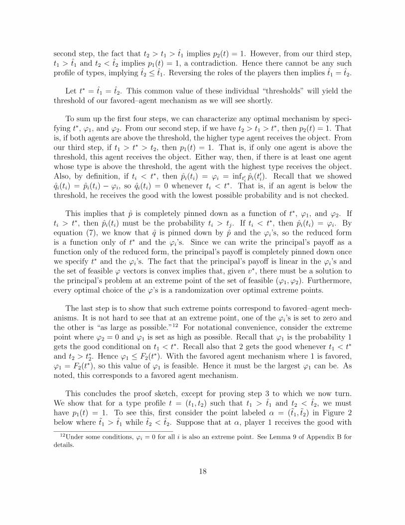
This concludes the proof sketch, except for proving step 3 to which we now turn.We show that for a type profile t = (t1, t2) such that t1 > t1 and t2 < t2, we musthave p1(t) = 1. To see this, first consider the point labeled α = (t1, t2) in Figure 2below where t1 > t1 while t2 < t2. Suppose that at α, player 1 receives the good with

12Under some conditions, ϕi = 0 for all i is also an extreme point. See Lemma 9 of Appendix B fordetails.

18

probability strictly less than 1. Then at any point directly below α but above t1, such asthe one labeled β = (t′1, t2), player 1 must receive the good with probability zero. Thisfollows because if 1 did receive the good with strictly positive probability here, we couldchange the mechanism by lowering this probability slightly, giving the good to 2 at βwith higher probability, and increasing the probability with which 1 receives the good atα. By choosing these probabilities appropriately, we do not affect p2(t2) so this remainsat ϕ2. Also, by making the reduction in p1 small enough, p1(t′1) will remain above ϕ1.Hence this new mechanism would be feasible. Since it would switch probability from onetype of player 1 to a higher type, the new mechanism would be better than the old one,implying the original one was not optimal.13

t1

t01

t1

t001

t2 t2 t02 t2

t1

p1 < 1

p1 = 0

p1 > 0

p1 > 0

p1 < 1

↵

�

�

�

"

Figure 2

Similar reasoning implies that for every t1 6= t1, we must have∑

i pi(t1, t2) = 1. Oth-erwise, the principal would be strictly better off increasing p2(t1, t2), decreasing p2(t1, t2),and increasing p1(t1, t2). Again, if we choose the sizes of these changes appropriately,p2(t2) is unchanged but p1(t1) is increased, an improvement.

Since player 1 receives the good with zero probability at β but type t′1 does have astrictly positive probability overall of receiving the good (as t′1 > t1), there must be somepoint like the one labeled γ = (t′1, t

′2) where 1 receives the good with strictly positive

13Since p2(t2) is unchanged, the ex ante probability of type t1 getting the good goes up by the sameamount that the ex ante probability of the lower type t′1 getting it goes down.

19

probability. We do not know whether t′2 is above or below t2 — the position of γ relativeto this cutoff plays no role in the argument to follow.

Finally, there must be a t′′1 6= t1 (not necessary below t1) corresponding to points δand ε where p1 is strictly positive at δ and strictly less than 1 at ε. To see that such at′′1 must exist, suppose not. Then for all t1 6= t1, either p1(t1, t2) = 0 or p1(t1, t

′2) = 1.

Since∑

i pi(t1, t2) = 1 for all t1 6= t1, this implies that for all t1 6= t1, either p2(t1, t2) = 1or p2(t1, t

′2) = 0. Either way, p2(t1, t2) ≥ p2(t1, t

′2) for all t1 6= t′1. But we also have

p2(t′1, t2) = 1 > 1 − p1(t′1, t′2) ≥ p2(t′1, t

′2). So p2(t2) > p2(t′2). But p2(t2) = ϕ2, so this

implies p2(t′2) < ϕ2, which violates the constraints on our optimization problem.

Now we use p1(t′′1, t2) > 0 and p1(t′′1, t′2) < 1 to derive a contradiction to the optimality

of the mechanism. Specifically, we change the specification of p at the points α, γ, ε,and δ in a way that lowers the probability that 1 gets the object at γ and raises theprobability he gets it at α by the same amount, while maintaining the constraints. Since1’s type is higher at α, this is an improvement, implying that the original mechanism wasnot optimal. Let ∆ > 0 be a “small” positive number. All the changes in p that we nowdefine involve increases and decreases by the same amount ∆. At γ, lower p1 and increasep2. At ε, do the opposite — i.e., raise p1 and lower p2. Because F1 is uniform, p2(t′2) isunchanged. Also, if ∆ is small enough, p1(t′1) remains above ϕ1. Thus the constraints aremaintained. Now that we have increased p1 at ε, we can decrease it at δ while increasingp2, keeping p1(t′′1) unchanged by the uniformity of F2. Finally, since we have increasedp2 at δ, we can decrease it at α while increasing p1, keeping p2(t2) unchanged. Note thatoverall effect of these changes is a reduction of ∆ in the probability that 1 gets the objectat γ and an increase of ∆ in the probability he gets the object at α, while maintainingall constraints.

This completes the sketch of the proof of Theorem 2. The proof itself is divided totwo parts. The main part, Theorem 5, establishes certain properties of every optimalmechanism. The proof of this result corresponds to steps (1) through (4) in the sketchabove and is contained in Appendix A. The proof of Theorem 2 from Theorem 5, step(5) in the proof sketch, is given in Appendix B.

6.2 Almost Dominance and Ex Post Incentive Compatibility

One appealing property of the favored–agent mechanism is that it is almost a dominantstrategy mechanism. That is, for every agent, truth telling is a best response to anystrategies by the opponents. It is not always a dominant strategy, however, as the agentmay be completely indifferent between truth telling and lies.

To see this, consider any agent i who is not favored and a type ti such that ti−ci > v∗.

20

If ti reports his type truthfully, then i receives the object with strictly positive probabilityunder a wide range of strategy profiles for the opponents. Specifically, any strategyprofile for the opponents with the property that ti − ci is the highest report for sometype profiles has this property. On the other hand, if ti lies, then i receives the objectwith zero probability given any strategy profile for the opponents. This follows becausei is not favored and so cannot receive the object without being checked. Hence for sucha type, truth telling weakly dominates any lie for ti.

Continuing to assume i is not favored, consider any ti such that ti − ci < v∗. Forany profile of strategies by the opponents, ti’s probability of receiving the object is zeroregardless of his report. To see this, simply note that if i reports truthfully, he cannotreceive the good (since it will either go to another nonfavored agent if one has the highesttj− cj and reports honestly or to the favored agent). Similarly, if i lies, he cannot receivethe object since he will be caught lying when checked. Hence truth telling is an optimalstrategy for ti, though it is not weakly dominant since the agent is indifferent over allreports given any strategies by the other agents.

A similar argument applies to the favored agent. Again, if his type satisfies ti−ci > v∗,truth telling is dominant, while if ti − ci < v∗, he is completely indifferent over allstrategies. Either way, truth telling is an optimal strategy regardless of the strategies ofthe opponents.

Because of this property, the favored–agent mechanism is ex post incentive compati-ble. Formally, (p, q) is ex post incentive compatible if

pi(t) ≥ pi(ti, t−i)− qi(ti, t−i), ∀ti, ti ∈ Ti, ∀t−i ∈ T−i, ∀i ∈ I.

That is, ti prefers reporting honestly to lying even conditional on knowing the types ofthe other agents. It is easy to see that the favored–agent mechanism’s almost–dominanceproperty implies this. Of course, the ex post incentive constraints are stricter than theBayesian incentive constraints, so this implies that that favored–agent mechanism is expost optimal.

While the almost–dominance property implies a certain robustness of the mechanism,the complete indifference for types below the threshold is troubling. There are simplemodifications of the mechanism which do not change its equilibrium properties but maketruth telling weakly dominant rather than just almost dominant. For example, supposethere are at least three agents and that every agent i satisfies ti − ci > v∗.14 Supposewe modify the favored– agent mechanism as follows. If an agent is checked and foundto have lied, then one of the other agents is chosen at random and his report is checked.

14Note that if ti− ci < v∗, then the favored agent mechanism never gives the object to i, so i’s reportis entirely irrelevant to the mechanism. Thus we cannot make truth telling dominant for such an agent,but the report of such an agent is irrelevant anyway.

21

If it is truthful, he receives the object. Otherwise, no agent receives it. It is easy to seethat truth telling is still an optimal strategy and that the outcome is unchanged if allagents report honestly. It is also still weakly dominant for an agent to report the truthif ti − ci > v∗. Now it is also weakly dominant for an agent to report the truth even ifti− ci < v∗. To see this, consider such a type and assume i is not favored. Then if ti lies,it is impossible for him to receive the good regardless of the strategies of the other agents.However, if he reports truthfully, there is a profile of strategies for the opponents wherehe has a strictly positive probability of receiving the good — namely, where one of thenonfavored agents lies and has the highest report. Hence truth telling weakly dominatesany lie. A similar argument applies to the favored agent.

6.3 Extensions

In this subsection, we discuss some simple extensions. First, it is straightforward togeneralize to allow the principal to have a strictly positive value, say R > 0, to retainingthe object. To see this, simply introduce an agent I+ 1 whose type is R with probability1. Allocating the object to this agent is the same as keeping it. It is easy to see thatour analysis then applies to this modified model directly. If R is sufficiently large, thenagent I + 1 will be favored. That is, if every agent i ≤ I reports ti − ci < R, then theprincipal retains the object. If any agent i ≤ I reports ti − ci > R, then the agent withthe highest such report is checked and, if found not to have lied, receives the object.This mechanism is the analog of a reserve price mechanism with R as the reserve price.If R is small enough that I + 1 is not the favored agent, then the optimal mechanism isunaffected by the principal’s value.

Another natural extension to consider is when the process of verifying an agent’sclaim is also costly for that agent. In our example where the principal is a dean and theagents are departments, it seems natural to say that departments bear a cost associatedwith providing documentation to the dean.

The main complication associated with this extension is that the agents may now tradeoff the value of obtaining the object with the costs of verification. An agent who valuesthe object more highly would, of course, be willing to incur a higher expected verificationcost to increase his probability of receiving it. Thus the simplification we obtain wherewe can treat the agent’s payoff as simply equal to the probability he receives the objectno longer holds.

On the other hand, we can retain this simplification at the cost of adding an assump-tion. To be specific, we can simply assume that the value to the agent of receiving theobject is 1 and the value of not receiving it is 0, regardless of his type. If we make thisassumption, the extension to verification costs for the agents is straightforward. We can

22

also allow the cost to the agent of being verified to differ depending on whether the agentlied or not. To see this, let cTi ≥ 0 be the cost incurred by agent i from being verifiedby the principal if he reported his type truthfully and let cFi ≥ 0 be his cost if he lied.We assume cTi < 1 to ensure that individual rationality always holds. The incentivecompatibility condition becomes

pi(t′i)− cTi qi(t′i) ≥ pi(ti)− cFi qi(ti)− qi(ti), ∀ti, t′i, ∀i.

Letϕi = inf

t′i

[pi(t′i)− cTi qi(t′i)],

so that incentive compatibility holds iff

ϕi ≥ pi(ti)− cFi qi(ti)− qi(ti), ∀ti, ∀i.

Analogously to the way we characterized the optimal mechanism in Section 6.1, we cantreat ϕi as a separate choice variable for the principal where we add the constraint thatpi(t

′i)− cTi qi(t′i) ≥ ϕi for all t′i.

Given this, qi(ti) must be chosen so that the incentive constraint holds with equalityfor all ti. To see this, suppose to the contrary that we have an optimal mechanism wherethe constraint holds with strict inequality for some ti (more precisely, some positivemeasure set of ti’s). If we lower qi(ti) by ε, the incentive constraint will still hold. Sincethis increases pi(t

′i) − cTi qi(t

′i), the constraint that this quantity is greater than ϕi will

still hold. Since auditing is costly for the principal, his payoff will increase, implying theoriginal mechanism could not have been optimal, a contradiction.

Since the incentive constraint holds with equality for all ti, we have

qi(ti) =pi(ti)− ϕi

1 + cFi. (10)

Substituting, this implies that

ϕi = inft′i

[pi(t

′i)−

cTi1 + cFi

[pi(ti)− ϕi]]

or

ϕi = inft′i

[{1− cTi

1 + cFi

}pi(ti) +

cTi1 + cFi

ϕi

].

By assumption, the coefficient multiplying pi(t′i) is strictly positive, so this is equivalent

to {1− cTi

1 + cFi

}ϕi =

{1− cTi

1 + cFi

}inft′i

pi(t′i),

so ϕi = inft′i pi(t′i), exactly as in our original formulation.

23

The principal’s objective function is

Et

∑i

[pi(t)ti − ciqi(t)] =∑i

Eti [pi(ti)ti − ciqi(ti)]

=∑i

Eti

[pi(ti)ti −

ci1 + cFi

[pi(ti)− ϕi]]

=∑i

Eti [pi(ti)(ti − ci) + ϕici]

where ci = ci/(1 + cFi ). This is the same as the principal’s objective function in ouroriginal formulation but with ci replacing ci.

Thus the solution changes as follows. The allocation probabilities pi are exactly thesame as what we characterized but with ci replacing ci. The checking probabilities,however, are the earlier ones divided by 1 + cFi (see equation (10)). Intuitively, sinceverification imposes costs on the agent in this model, the threat of verification is moresevere than in the previous model, so the principal doesn’t need to check as often.

That is, the new optimal mechanism is still a favored–agent mechanism but wherethe checking which had probability 1 before now has probability 1/(1+ cFi ). The optimalchoice of the favored agent and the optimal threshold is exactly as before with ci replacingci. Note that agents with low values of cFi have higher values of ci and hence are morelikely to be favored. That is, agents who find it easy to undergo an audit after lying aremore likely to be favored. Note also that cTi has no effect on optimal mechanism.

As a third extension, suppose that the principal can impose (limited) fines on theagents. Assume, as in the second extension, that the value to an agent of receiving theobject is 1 and the payoff to not receiving it is zero. It is easy to see that the optimalmechanism for the principal is impose the largest possible fine when the agent is foundto have lied and nothing otherwise. The analysis of this model is then identical to thatof our second extension where we set cTi = 0 and cFi equal to this maximum penalty.

7 Conclusion

There are many natural extensions to consider. For example, in the previous subsec-tion, we discussed the extension in which the agents bear some costs associated withverification, but under the restriction that the value to the agent of receiving the ob-ject is independent of his type. A natural extension of interest would be to drop thisrestriction.15

15See Ambrus and Egorov (2012) for an analysis of how imposing costs on agents can be useful forthe principal in a setting without verification.

24

A second natural extension would be to allow costly monetary transfers. We argued inthe introduction that within organizations, monetary transfers are costly to use and hencehave excluded them from the model. It would be natural to model these costs explicitlyand determine to what extent the principal allows inefficient use of some resources toobtain a better allocation of other resources.

Another direction to consider is to generalize the nature of the principal’s allocationproblem. For example, what is the optimal mechanism if the principal has to allocatesome tasks, as well as some resources? In this case, the agents may prefer to not re-ceive certain “goods.” Alternatively, there may be some common value elements to theallocation in addition to the private values aspects considered here.

In the context of the example of the dean allocating a job slot to one of severaldepartments, a natural extension would be to allow each department to have multiplecandidates, one of which it can put forward. In this case, the department faces a tradeoffbetween those the dean would prefer and those the department wants most. This tradeoffimplies that the value to the department of receiving the slot matters, unlike in theanalysis here. Thus this model would look more like a multiple sender version of Che,Dessein, and Kartik (forthcoming) with costly verification.

Another natural direction to consider is alternative specifications of the informationstructure and verification technology. Here each agent knows exactly what value he cancreate for the principal with the object. Alternatively, the principal may have privateinformation which determines how he interprets an agent’s information. Also, it is naturalto consider the possibility that the principal partially verifies an agent’s report, choosinghow much detail to go into. For example, an employer dealing with a job applicant candecide how much checking to do of the applicant’s resume and references.

25

Appendix

A Proof of Theorem 5

In this section, we state and prove a theorem which is used in Appendix B to proveTheorem 2. Specifically, in Theorem 5 below, we show that every optimal mechanism iswhat we call a threshold mechanism. In Appendix B, we show that optimal thresholdmechanisms are convex combinations of favored–agent mechanisms. In this and subse-quent sections, we work with the restated version of the optimization problem for theprincipal derived in Section 6.1 (in particular, equations (8) and (9) and the constraintsthat follow).

Definition 1. (p, q) is a threshold mechanism if there exists v∗ ∈ R such that thefollowing holds for all t up to sets of measure zero. First, if there exists any i withti − ci > v∗, then pi(t) = 1 for that i such that ti − ci > maxj 6=i(tj − cj). Second, for alli, if ti − ci < v∗, then qi(t) = 0 and pi(ti) = mint′i∈Ti pi(ti).

Theorem 5. Every optimal mechanism is a threshold mechanism.

The proof of Theorem 5 proceeds with a series of lemmas. Throughout we write thedistribution of ti as a measure µi. Recall that we have assumed this measure is absolutelycontinuous with respect to Lebesgue measure on the interval Ti ⊂ R. We let µ be theproduct measure on the product Borel field of T . For any S ⊆ T , let

S(ti) = {t−i ∈ T−i | (ti, t−i) ∈ S}

denote the ti fiber of S. Let Si denote the projection of S on Ti, and S−ij the projectionon∏

k 6∈{i,j} Tk.

We begin with a technical lemma.16

Lemma 1. Given any Borel measurable S ⊂ RI with µ(S) > 0, there exists S∗ ⊆ Swith µ(S∗) = µ(S) such that the following holds. First, for every i and every ti ∈ Ti, themeasure of every fiber is strictly positive. That is, µ−i(S(ti)) > 0 for all i and all ti ∈ Ti.Second, for all i, the projection on i of S∗, S∗i , is measurable.

Moreover, given any j, there exists ε > 0 and S∗∗ ⊆ S with µ(S∗∗) > 0 such that thefollowing holds. First, for every i 6= j and every ti ∈ Ti, the measure of every fiber isstrictly positive. That is, µ−i(S

∗∗(ti)) > 0. Second, for every tj ∈ S∗∗j , the fiber S∗∗(tj)has measure bounded below by ε. That is, µ−j(S

∗∗(tj)) > ε. Finally, for all i, S∗∗i , theprojection on i of S∗∗, is measurable.

16We thank Benjy Weiss for suggesting the idea of of the following proof.

26

Proof. We first prove this for I = 2, and then show how to extend it to I > 2. So, tosimplify notation for the first step, denote by x and y the two dimensions. Fix a Borelmeasurable S with µ(S) > 0. We need to show that there is an equal measure subset ofS, S∗, such that all fibers of S∗ have strictly positive measure and all projections of S∗

are measurable. So we need to show (1) µx(S∗(y)) > 0 for all y, (2) µy(S

∗(x)) > 0 for allx, and (3) the projections of S∗ are measurable.

First, we observe that if all the fibers have strictly positive measure, then the pro-jections are measurable. To see this, note that the function f : X → R given byf(x) = µy(S

∗(x)) is measurable by Fubini’s Theorem. Hence the set {x | µy(S∗(x)) > 0}is measurable. But this is just the projection on the first dimension if the fiber haspositive measure. An analogous argument applies to the y coordinate.

Let S1 denote the set S after we delete all x fibers with µy measure zero. That is,S1 = S ∩ [{x | µy(S(x)) > 0} × R]. We know that S1 is measurable, has the samemeasure as S (by Fubini, because we deleted only fibers of zero measure), all its x fibershave strictly positive y measure, and its projection on x is measurable.

We do not know that the projection of S1 on y is measurable nor that the y fibershave strictly positive x measure. Let S2 denote the set S1 after we delete all y fiberswith µx measure zero. That is, S2 = S1 ∩ [{y | µx(S1(y)) > 0} ×R]. We know that S2

is measurable with the same measure as S1, that its projection on y is measurable, andall its y fibers have strictly positive y measure.

Again, we do not know that its projection on x is measurable nor that the x fibershave strictly positive y measure. But at this step we do know that the set of x fibersthat have zero measure is contained in a set of measure zero. Put differently,

µx{x | µy

(S2(x)

)> 0}

= µx(S1x

)= µx

{x | µy

(S1 (x)

)> 0}. (11)

To see this, suppose not. Then

µx{x | µy

(S2 (x)

)> 0}< µx

{x | µy

(S1 (x)

)> 0}

as {x | µy

(S2 (x)

)> 0}⊆{x | µy

(S1 (x)

)> 0}.

Let∆ =

{x | µy

(S1 (x)

)> 0}\{x | µy

(S2 (x)

)> 0}.

27

If µ(∆) > 0, then

µ(S1)

=

∫{x|µy(S1(x))>0}

µy(S1 (x)

)µx (dx)

=

∫{x|µy(S2(x))>0}

µy(S1 (x)

)µx (dx) +

∫∆

µy(S1 (x)

)µx (dx)

>

∫{x|µy(S2(x))>0}

µy(S2 (x)

)µx (dx)

= µ(S2)

as S1(x) ⊇ S2(x) and µ(∆) > 0. But this contradicts µ(S2) = µ(S1). Hence equation(11) holds.

Finally, let S3 denote S2 after we delete all x fibers with µy measure zero. That is,S3 = S2 ∩ [{x | µy(S2(x)) > 0} × R]. We know that S3 is measurable with the samemeasure as S2, that its projection on x is measurable, and that all its x fibers have strictlypositive y measure. But now we also know that all the y fibers have strictly positive xmeasure, since in going from S2 to S3, we deleted a set of x’s contained in a set of zeromeasure. Hence each y fiber has the same measure as before.

We now extend this to I > 2. For brevity, we only describe the extension to I = 3,the more general result following the same lines. Denote the coordinates by x, y, and z.Consider a set S with µ(S) > 0. We show there exists S∗ ⊆ S such that µyz(S

∗(x)) > 0for all x ∈ S∗x, and similarly for all y ∈ S∗y and all z ∈ S∗z .

From the case of I = 2, we know there exists S1 ⊆ S with µ(S1) = µ(S) such that forall x ∈ S1

x, we have µyz(S1(x)) > 0 and for all (y, z) ∈ S1

yz, we have µx(S1((y, z))) > 0.

Applying I = 2 result again to the set S1yz, we have G ⊆ S1

yz with µyz(G) = µyz(S1yz)

such that for all y ∈ Gy, we have µz(G(y)) > 0 and for all z ∈ Gz, we have µy(G(z)) > 0.(Note that this implies that µyz(G) > 0.)

Now define

S2 = S1 ∩ (R×G) ={

(x, y, z) | (x, y, z) ∈ S1 and (y, z) ∈ G}.

Since G ⊆ S1yz and µyz(G) = µyz(S

1yz), we have µ(S2) = µ(S1). Clearly, S2

y = Gy andS2z = Gz. Fix any y ∈ S2

y . Since y ∈ Gy, we have µz{z | (y, z) ∈ G} > 0. Since G ⊆ S1yz

for every (y, z) ∈ G, we have µx(S2(y, z)) = µx(S

1(y, z)) > 0. By Fubini’s Theorem,µxz(S

2(y)) =∫z∈G(y)

µx(S2(y, z))µz(dz) and hence µxz(S

2(y)) > 0. A similar argument

implies that for all z ∈ S2(z), we have µxy(S2(z)) > 0. However, we do not know that

for every x ∈ S2x, we have µy,z(S

2(x)) > 0. Hence we now define the set S3 by

S3 = S2 ∩({x | µyz(S2(x)) > 0

}×R2

).

28

Clearly, S3x is measurable and we have µyz(S

3(x)) > 0 for every x ∈ S3x. Furthermore,

S3 ⊆ S2 ⊆ S1 and hence S3x ⊆ S1

x. In fact, µ(S3) = µ(S2) = µ(S1) implies µ(S3x) = µ(S1

x).To see this, suppose not. Then µx(S

3x) < µx(S

1x). Since for each x ∈ S1

x, we haveµyz(S

1(x)) > 0, we obtain that µ(S3) < µ(S1), a contradiction.

We claim that S3 satisfies the properties stated in the first part of the lemma. Thatis, (1) S3

y and S3z are measurable, (2) for all y ∈ S3

y , we have µx,z(S3(y)) > 0, and (3)

for all z ∈ S3z , we have µx,y(S

3(z)) > 0. Consider an element y ∈ S2y . We have seen

that for all z ∈ G(y), we have µx(S2(y, z)) > 0. Since our construction of S3 removes

from S2 a set of elements x in S2x that is contained in a set of measure zero, we must

have µx(S3(y, z)) = µx(S

2(y, z)) > 0. Hence S3y = S2

y and for every y ∈ S3y , we have

µxz(S3(y)) = µxz(S

2(y)) > 0. A similar argument establishes that S3z = S2

z and thatfor z ∈ S3

z , we have µxy(S3(y)) > 0. By defining S∗ = S3, we obtain a set S∗ with the

properties claimed in the first part of the lemma.

It remains to prove the “moreover” claim. This follows from a similar argument wherein defining S1, we remove all x’s whose fibers do not have probability at least ε for anappropriately chosen ε. We provide the proof for the case I = 2. The proof for I > 2 issimilar.

Note that

{x | µy(S(x)) > 0} =∞⋃n=1

{x | µy(S(x)) > 1/n} .

Since µx({x | µy(S(x)) > 0}) > 0, there exists n such that µx({x | µy(S(x)) > 1/n}) > 0.Define ε = 1/n and define S1 = S ∩ ({x | µy(S(x)) > ε} ×R).

The rest of the argument is essentially identical to the argument given in the proofof the first part of the lemma. Specifically, we know that S1

x is measurable and that forevery x ∈ S1

x, we have µy(S1(x)) > ε. Define

S2 = S1 ∩({y | µx(S1(y)) > 0

}×R

)S3 = S2 ∩

({x | µy(S2(x)) > ε

}×R

).

We have S3 ⊆ S2 ⊆ S1. Fubini’s Theorem implies that µ(S2) = µ(S1) which in turnimplies that

µx({x | µy(S2(x)) > ε

}) = µx(

{x | µy(S1(x)) > ε

}).

To see this, suppose not. Then S2 ⊆ S1 and the fact that µy(S1(x)) > ε for all x ∈ S1

x

implies that µ(S2) < µ(S1), a contradiction.

Since {x | µy(S2(x)) > ε

}={x | µy(S3(x)) > ε

}= S3

x,

29

we see that µx(S1x) = µx(S

3x). Hence in moving from S2 to S3, the set of x’s that is

deleted is contained in a set of measure zero. Since for all y ∈ S2y , we have µx(S

2(y)) > 0,we see that S3

y = S2y and that µx(S

3(y)) > 0 for all y ∈ S3y . Thus the set S3 satisfies all

the properties stated in the second paragraph of the lemma.

For the remaining lemmas, fix p and ϕ that maximize

Et

[∑i

[pi(t)(ti − ci) + ϕici]

]=∑i

{Eti [pi(ti)(ti − ci)] + ϕici]}

subject to∑

i pi(t) ≤ 1 for all t and pi(ti) ≥ ϕi ≥ 0 for all i and ti where pi(ti) = Et−ipi(t).

As explained in Section 6.1, the optimal q will then be any feasible q satisfying qi(ti) =pi(ti)− ϕi for all i and ti where qi(ti) = Et−i

qi(t).

Lemma 2. There is a set T ′ ⊆ T with µ (T ′) = 1 such that the following hold:

1. For each i, if ti < ci and ti ∈ T ′i , then pi(ti) = ϕi.

2. For each t ∈ T ′, if ti > ci for some i, then∑

j pj(t) = 1.

3. For any t ∈ T ′, if pi(ti) > ϕi for some i, then∑

j pj(t) = 1.

Proof. Proof of 1. If ti < ci, then the objective function is strictly decreasing in pi(ti).Obviously, reducing pi(ti) makes the other constraints easier to satisfy. Since we improvethe objective function and relax the constraints by reducing pi(ti), we must have pi(ti) =ϕi at the optimum. This completes the proof of part 1. Since we only characterizeoptimal mechanisms up to sets of measure zero, we abuse notation, and redefine T toequal a measure 1 subset of T on which property 1 is satisfied, and whose projections aremeasurable (which exists by Lemma 1).

Proof of 2. Suppose not. Then there exists an agent i and a set T with positivemeasure such that for every t ∈ T , we have ti > ci and yet

∑j pj(t) < 1. Define an

allocation function p∗ by

p∗j(t) =

{pj(t), if j 6= i or t /∈ T1−

∑j 6=i pj(t), otherwise.

It is easy to see that p∗ satisfies all the constraints and improves the objective function,a contradiction.

Proof of 3. Suppose to the contrary that we have a positive measure set of t such that∑j pj(t) < 1 but for each t, there exists some i with pi(ti) > ϕi. Then there exists i and

a positive measure set of t such that for each t, we have∑

j pj(t) < 1 and pi(ti) > ϕi.

30

From part 1, we know that for all ti ∈ Ti with pi(ti) > ϕi we have ti > ci. Hence frompart 2, the mechanism is not optimal, a contradiction.

Abusing notation, redefine T to equal a measure 1 subset of T \ T ′ whose projectionsare measurable (which exists by Lemma 1) on which all the properties of Lemma 2 aresatisfied everywhere.

Lemma 3. There is a set T ′ ⊆ T with µ(T ′) = 1 such that for any t ∈ T ′, if ti−ci > tj−cjand pj(tj) > ϕj, then pj(t) = 0.

Proof. Suppose not. Then we have a positive measure set S such that for all t ∈ S,ti − ci > tj − cj, pj(tj) > ϕj, and pj(t) > 0. Hence there exists α > 0 and ε > 0 such

that µ(S) > 0 where

S = {t ∈ T | ti − ci − (tj − cj) ≥ α, pj(tj) ≥ ϕj + ε, and pj(t) ≥ ε}.

Define p∗ by

p∗j(t) =

pk(t), for k 6= i, j or t /∈ Spj(t)− ε, for k = j and t ∈ Spi(t) + ε, for k = i and t ∈ S.

Since pj(t) ≥ ε for all t ∈ S, we have p∗k(t) ≥ 0 for all k and t. Obviously,∑

k p∗k(t) =∑

k pk(t), so the constraint that the pk’s sum to less than one must be satisfied.

Turning to the lower bound constraint on the pk’s, obviously, for k 6= j, we havep∗k(tk) ≥ pk(tk) ≥ ϕk, so the constraint is satisfied for all k 6= j and all tk. For any tj,either p∗j(tj) = pj(tj) or

p∗j(tj) = pj(tj)− εµ−j(S (tj)) ≥ pj(tj)− ε.

But for each tj for which p∗j(tj) 6= pj(tj), we have pj(tj) ≥ ϕj + ε, so

p∗j(tj) ≥ ϕj + ε− ε = ϕj.

Hence for every k and every tk, we have p∗k(tk) ≥ ϕk. Therefore, p∗ is feasible given ϕ.

Finally, the change in the principal’s payoff in moving from p to p∗ is

µ(S)ε[E(ti − ci | t ∈ S)− E(tj − cj | t ∈ S)

]≥ µ(S)εα > 0.

Hence p could not have been optimal, a contradiction.

Thus the set S0 = {t ∈ T | ti − ci − (tj − cj) > 0, pj(tj) > ϕj, and pj(t) > 0} hasmeasure zero. Abusing notation, redefine T to equal a measure 1 subset of T \ S0 whoseprojections are measurable (which exists by Lemma 1).

31

Lemma 4. There is a set of measure one T ′ ⊆ T such that for all t′, t′′ ∈ T ′ such thatt′j = t′′j , pj(t

′) > 0, pi(t′i) > ϕi, t

′′i < t′i, and pi(t

′′i ) > ϕi, we have pi(t

′′) = 0.

The idea that underlies the proof is simple. Consider two profiles t′ and t′′ that havethe properties stated in the lemma. That is, t′j = t′′j , pj(t

′) > 0, pi(t′i) > ϕi, t

′′i < t′i, and

pi(t′′i ) > ϕi. Suppose the claim is false, so that pi(t

′′) > 0. Clearly, there is some ε > 0such that pj(t

′) > ε, pi(t′i) > ϕi + ε, and pi(t

′′i ) > ϕi + ε, and pi(t

′′) > ε. For simplicity,assume µ(t′) = µ(t′′) = δ > 0. (The formal proof will extend the argument to the casethat µ is a general atomless probability measure.) Consider the following transfer ofallocation probabilities between agents i and j. For the profile t′, increase pi(t

′) by εand decrease pj(t

′) by ε. For the profile t′′, decrease pi(t′′) by ε and increase pj(t

′′) by ε.Let p∗ denote the resulting probability function. It is easy to see that p∗ satisfies all theconstraints. Also, it increases the value of the objective function because the net effectof the transfers is to move a probability εδ of allocating the object from type t′′i to typet′i where t′i > t′′i . This argument is not sufficient for the general proof, of course, since µis atomless, implying that we must change p on a positive measure set of types to havean effect.

Proof. Given any rational number α and any t′j ∈ Tj, let

A−j(α, t′j) = {t′−j ∈ T−j | t′i > α, pi(t

′i) > ϕi, and pj(t

′) > 0}

B−j(α, t′j) = {t′−j ∈ T−j | t′i < α, pi(t

′i) > ϕi, and pi(t

′) > 0}.

Cj(α) = {t′j ∈ Tj | µ−j(A−j(α, t′j)) > 0, µ−j(B−j(α, t′j)) > 0}.

Also let

A−j(α, t′j, ε, δ) = {t′−j ∈ T−j | t′i > α + δ, pi(t

′i) > ϕi + ε, and pj(t

′) > ε}

B−j(α, t′j, ε, δ) = {t′−j ∈ T−j | t′i < α− δ, pi(t′i) > ϕi + ε, and pi(t

′) > ε}.

and

A(α, ε, δ) = {t ∈ T | ti > α + δ, pi(ti) > ϕi + ε, and pj(t) > ε}

=⋃t′j∈Tj

{t′j}× A−j(α, t′j, ε, δ)

B(α, ε, δ) = {t ∈ T | ti < α− δ, pi(ti) > ϕi + ε, and pi(t) > ε}

=⋃t′j∈Tj

{t′j}× B−j(α, t′j, ε, δ)

Cj(α, ε, δ) = {t′j ∈ Tj | µ−j(A−j(α, t′j, ε, δ)) > 0, µ−j(B−j(α, t′j, ε, δ)) > 0}.

32

Finally let

A (α, ε, δ) =⋃

tj∈Cj(α,ε,δ)

{tj} × A−j(α, tj, ε, δ) =(Cj (α, ε, δ)× T−j

)∩ A (α, ε, δ)

B (α, ε, δ) =⋃

tj∈Cj(α,ε,δ)

{tj} × B−j(α, tj, ε, δ) =(Cj (α, ε, δ)× T−j

)∩ B (α, ε, δ)

Measurability of all the sets defined above follows from standard arguments.

We now show that for every rational number α, we have µj(Cj(α)) = 0. So supposenot. Fix the rational α for which it fails. Then there must be ε > 0 and δ > 0 such thatµj(Cj(α, ε, δ)) > 0. For notational simplicity, we drop the arguments α, ε, δ in the nextstep of the argument as they are fixed in this step.

Define p∗ as follows. For k 6= i, j and any t, p∗k(t) = pk(t). Also, for any t /∈ A ∪ Band all k, p∗k(t) = pk(t). For t ∈ A,

p∗j(t) = pj(t)− εµ−j(B−j (tj)

)and p∗i (t) = pi(t) + εµ−j

(B−j(tj)

).

For t ∈ B,

p∗j(t) = pj(t) + εµ−j

(A−j (tj)

)and p∗i (t) = pi(t)− εµ−j

(A−j (tj)

).

For t ∈ A, we have pj(t) ≥ ε, while for t ∈ B, pi(t) ≥ ε. Hence p∗ satisfies non–negativity. Clearly, for any t,

∑k p∗k(t) =

∑k pk(t), so p∗ satisfies the constraint that the

sum of the p’s is less than 1.

Obviously, for k 6= i, j, we have p∗k(tk) = pk(tk) ≥ ϕk. So the lower bound constrainton pk(tk) holds for all tk for all k 6= i, j. Clearly, for any tj such that p∗j(t) ≥ pj(t) for allt−j, we have pj(tj) ≥ ϕj. Otherwise, we have

p∗j(tj) = pj(tj)− εµ−j(B−j(tj)

)µ−j(A(tj)) + εµ−j

(B−j(tj)

)µ−j

(A−j (tj)

).

So p∗j(tj) = pj(tj). Hence p∗j(tj) ≥ ϕj for all tj ∈ Tj.

For any ti such that p∗i (t) ≥ pi(t) for all t−i, we have pi(ti) ≥ ϕi. So consider tisuch that p∗i (t) < pi(t) for some t−i. Then there must be t−i such that t ∈ B. Hencepi(ti) ≥ ϕi + ε. So

p∗i (ti) = pi(ti) + εµ−i({t−i | (ti, t−i) ∈ A}

)µ−j

(B−j (tj)

)− εµ−i

({t−i | (ti, t−i) ∈ B}

)µ−j

(A−j (tj)

)≥ pi(ti)− ε≥ ϕi + ε− ε = ϕi.

33

Hence the lower bound constraint for pi also holds everywhere.

Finally, the change in the principal’s payoff from switching to p∗ from p is∫t∈A

{[(ti − ci)εµ−j

(B−j(tj)

)]−[(tj − cj)εµ−j

(B−j(tj)

)]}µ(dt)

+

∫t∈B

{[−(ti − ci)εµ−j

(A−j(tj)

)]+[(tj − cj)εµ−j

(A−j(tj)

)]}µ(dt)

=

∫Cj

(∫A−j(tj)

{[(ti − ci)εµ−j

(B−j(tj)

)]−[(tj − cj)εµ−j

(B−j(tj)

)]}µ−j(dt−j)

+

∫B−j(tj)

{[−(ti − ci)εµ−j

(A−j(tj)

)]+[(tj − cj)εµ−j

(A−j(tj)

)]}µ−j(dt−j)

)µj(dtj).

Note that (tj − cj)εµ−j(A−j(tj)) and (tj − cj)εµ−j(B−j(tj)) are functions only of tj, nott−j. Hence we can rewrite the above as∫

Cj

(−[(tj − cj)εµ−j

(B−j(tj)

)] ∫A−j(tj)

µ−j(dt−j)

)µj(dtj)

+

∫Cj

([(tj − cj)εµ−j

(A−j(tj)

)] ∫B−j(tj)

µ−j(dt−j)

)µj(dtj)

+

∫Cj

(∫A−j(tj)

[(ti − ci)εµ−j

(B−j(tj)

)]µ−j(dt−j)

)µj(dtj)

−∫Cj

(∫B−j(tj)

[(ti − ci)εµ−j

(A−j(tj)

)]µ−j(dt−j)

)µj(dtj)

The first two lines sum to zero. For the last two lines, recall that t ∈ A implies ti ≥ α+δ,while t ∈ B implies ti ≤ α− δ. Hence the last two lines sum to at least∫

Cj

(∫A−j(tj)

[(α + δ)εµ−j

(B−j(tj)

)]µ−j(dt−j)

)µj(dtj)

−∫Cj

(∫B−j(tj)

[(α− δ)εµ−j

(A−j(tj)

)]µ−j(dt−j)

)µj(dtj)

=

∫Cj

[(α + δ)εµ−j

(B−j(tj)

)µ−j

(A−j(tj)

)]µj(dtj)

−∫Cj

[(α− δ)εµ−j

(A−j(tj)

)µ−j

(B−j(tj)

)]µj(dtj)

> 0.

34

Hence the payoff difference for the principal between p∗ and p is strictly positive. Hencep could not have been optimal, a contradiction.

This establishes that for every rational α, µj(Cj(α)) = 0.

To complete the proof, let

Aj(α) = {tj ∈ Tj | µ−j(A−j(α, tj)) = 0}

andBj(α) = {tj ∈ Tj | µ−j(B−j(α, tj)) = 0}.

It is easy to see that for any α, Aj(α) ∪ Bj(α) ∪ Cj(α) = Tj. Let

A(α) =⋃

tj∈Aj(α)

{tj} × A−j(α, tj)

= {t ∈ T | ti > α, pi(ti) > ϕi, and pj(t) > 0} ∩[Aj (α)× T−j

]

B(α) =⋃

tj∈Bj(α)

{tj} × B−j(α, tj)

= {t ∈ T | ti < α, pi(ti) > ϕi, and pi(t) > 0} ∩[Bj (α)× T−j

]C(α) =

⋃tj∈Cj(α)

{tj} × T−j

andD(α) = A(α) ∪ B(α) ∪ C(α).

Once again measurability of the sets just defined is straightforward.

Note that µ (A (α)) = 0, since

µ(A(α)) =

∫Aj(α)

µ−j(A−j(α, tj))µj(dtj)

=

∫Aj(α)

µ−j(A−j(α, tj))µj(dtj)

= 0,

where the last equality follows from µ−j(A−j(α, tj)) = 0 for all tj ∈ Aj(α). Similarly,

µ(B(α)) = 0. Also, µ(C(α)) = µj(Cj(α))µ−j(T−j) which is 0 by the first step. Henceµ(D(α)) = 0.

35

Let S = ∪α∈QD(α) where Q denotes the rationals. Clearly µ(S) = 0.

To complete the proof, suppose that, contrary to our claim, there exists t′, t′′ ∈ T \ Ssuch that pj(t

′) > 0, pi(t′i) > ϕi, t

′′i < t′i, and pi(t

′′i ) > ϕi, but pi(t

′j, t′′i , t′′−ij) > 0.

Obviously, there exists a rational α such that t′′i < α < t′i. Hence (t′i, t′−ij) ∈ A−j(α, t′j)

and (t′′i , t′′−ij) ∈ B−j(α, t′j). Since t′ is not in S, we know that t′ /∈ A(α), implying that

t′j /∈ Aj(α). Similarly, since t′′ is not in S, we have t′′ /∈ B(α), so t′j /∈ Bj(α). Similarly,

t′ /∈ C(α), implying t′j /∈ Cj(α). But Aj(α) ∪ Bj(α) ∪ Cj(α) = Tj, a contradiction.

Abusing notation, define T to be a measure one subset of T ′ whose projections aremeasurable and such that for all t′, t′′ ∈ T for which t′j = t′′j , pj(t

′) > 0, pi(t′i) > ϕi,

t′′i < t′i, and pi(t′′i ) > ϕi, we have pi(t

′′) = 0.

Lemma 5. There is a set of measure one T ′ such that if pj(tj) = ϕj, pi(ti) > ϕi, and

µi ({t′i ∈ Ti | t′i < ti and pi(t′i) > ϕi}) > 0,

then pj(t) = 0.

Proof. Let

T ∗i = {ti ∈ Ti | pi(ti) > ϕi and µi({t′i | pi(t′i) > ϕi and t′i < ti}) > 0} .

To see that T ∗i is measurable. note that

T ∗i = T ∗i⋂{ti ∈ Ti | pi(ti) > ϕi}

whereT ∗i = {ti ∈ Ti | µi({t′i | pi(t′i) > ϕi and t′i < ti}) > 0} .

Since T ∗i is an interval (i.e., ti ∈ T ∗i and t′′i > ti implies t′′i ∈ T ∗i ), it is measurable. HenceT ∗i is the intersection of two measurable sets and so is measurable.

Suppose the claim of the lemma is not true. Then there exists ε > 0 such thatµ(S) > 0 and such that S has measurable projections where

S = {t ∈ T | ti ∈ T ∗i , pj(tj) = ϕj, pi (ti) > ϕi + ε, and pj(t) ≥ ε},

and where we use Lemma 1 and take an equal measure subset if necessary.

Since µ(S) > 0, we must have µi(Si) > 0 and hence µi(T∗i ) > 0 since Si ⊆ T ∗i . Choose

measurable sets Li,Mi, Ui ⊂ Si such that the following hold. First, all three sets havestrictly positive measure. Second, supLi < inf Mi and supMi < inf Ui. (Think of U , M ,

36

and L as standing for “upper,” “middle,” and “lower” respectively.) Third, there is anε′ > 0 such that µ(S) > 0 where S is defined as follows. Let

S ′′ =⋃ti∈Ui

{ti}×{t−i ∈ T−i | (ti, t−i) ∈ S} = {t ∈ T | ti ∈ Ui, pj(tj) = ϕj, and pj(t) ≥ ε}.

Clearly µ(S ′′) > 0. By Lemma 1, there exists a positive measure set S ⊂ S ′′ and a numberε′ > 0 satisfying the following. First, S has strictly positive measure fibers. That is, forall i and all ti, µ−i(S(ti)) > 0. Second, the j fibers of S have measure bounded below byε′. That is, µ−j(S(tj)) > ε′.

Let E = {t ∈ T | pi (t) > ϕi, ti ∈ Li}. Since pi (ti) > ϕi for all ti ∈ Li ⊂ T ∗i , E hasstrictly positive measure. By taking a subset if necessary, we know that for all k, theprojections Ek on Tk have strictly positive measure, as do the projections on −i and on−{i, j}. (E−i(ti) denotes, as usual, the ti fiber of E.)

Let A = Mi × E−i. Since µi(Mi) > 0 and µ−i(E−i) > 0, we see that µ(A) > 0.Taking subsets if necessary, and using Lemma 1, we know that we can find an equalmeasure subset (also, abusing notation, denoted A) all of whose fibers have strictlypositive measure and whose projections are measurable. We now show that pi(t) = 1 foralmost all t ∈ A.

To see this, suppose not. Then we have a positive measure set of such t ∈ A withpi(t) < 1. For all t ∈ A, we have pi(ti) > ϕi. In light of Lemma 2, this implies∑

k pk(t) = 1. Therefore, there exists k 6= i and a positive measure set A ⊆ A such that

pk(t) > 0 for all t ∈ A.

But fix any t′ ∈ A. By construction, t′i ∈ Mi and t′−i ∈ E−i(t′′i ) for some t′′i ∈ Li.

Since t′i ∈ Mi and t′′i ∈ Li, we have t′i > t′′i , pi(ti) > ϕi, and pi(t′′i ) > ϕi. By definition

of E−i(t′′i ), we have pi(t

′′i , t′−i) > 0. Finally, we have pk(t

′) > 0. Letting t′′ = (t′′i , t′−i), we

see that this is impossible given that we removed the set S defined in Lemma 4 from T .Hence pi(t) = 1 for all t ∈ A.

Let B = Mi × Sj ×E−ij. Recall that µi(Mi) > 0. Also, µ(S) > 0 implies µj(Sj) > 0.Finally, µ−ij(E−ij) > 0. Hence µ(B) > 0. Again, taking subsets if necessary, and usingLemma 1, we know that we can find an equal measure subset (also, abusing notation,denoted B) all of whose fibers have strictly positive measure and whose projections aremeasurable. We now show that for all t ∈ B, we have pj(t) = 1.

To see this, suppose not. Just as before, Lemma 2 then implies that there exists k 6= jand B ⊆ B such that for all t ∈ B, pk(t) > 0. First, we show that k 6= i. To see this,suppose to the contrary that k = i. Fix any t′′ ∈ B. By assumption, pi(t

′′) > 0. Bydefinition of B, t′′i ∈ Mi, so pi(t

′′i ) > ϕi. Also by definition of B, t′′j ∈ Sj. So fix t′ ∈ S

37

such that t′j = t′′j . By definition of S, t′i ∈ Ui, implying both pi(t′i) > ϕi and t′i > t′′i (as

t′′i ∈Mi). The definition of S also implies pj(t′) > 0. Just as before, this contradicts the

removal of S from T . Hence k 6= i.

So fix any t′ ∈ B. By assumption, pk(t′) > 0. By definition of B, t′i ∈ Mi, so

pi(t′i) > ϕi. Also, the definition of B implies that t′−ij ∈ E−ij(t′′i ) for some t′′i ∈ Li. Hence

there exists t′′j such that (t′′j , t′−ij) ∈ E−i(t

′′i ). Let t′′ = (t′′i , t

′′j , t′−ij). By construction,

t′k = t′′k. Also, since t′′i ∈ Li, we have pi(t′′i ) > ϕi and t′i > t′′i (as t′i ∈ Mi). Finally, by

definition of E−i(t′′i ), we have pi(t

′′) > 0. Again, this contradicts the removal of S fromT . Hence for all t ∈ B, pj(t) = 1.

Summarizing, for every t ∈ A, we have pi(t) = 1 (and hence pj(t) = 0) and pi(ti) ≥ϕi + ε, while for almost every t ∈ B, we have pj(t) = 1 and and pi(ti) ≥ ϕi + ε.

For any t′j ∈ Aj and t′′j ∈ Bj, let

F−j(t′j, t′′j ) = {t−j ∈ T−j | pj(t′j, t−j) > pj(t

′′j , t−j)}.

Obviously, for every tj and hence every tj ∈ Aj, we have pj(tj) ≥ ϕj. For every tj ∈ Bj,

we have tj ∈ Sj ⊆ Sj, so pj(tj) = ϕj. Hence for every t′j ∈ Aj and t′′j ∈ Bj, wehave pj(t

′j) ≥ pj(t

′′j ) even though pj(t

′) = 0 and pj(t′′) = 1 for all t′ ∈ A, t′′ ∈ B.

Moreover, B−j = A−j = Mi × E−i,j. Hence for every t′j ∈ Aj and t′′j ∈ Bj, we must haveµ−j(F−j(t

′j, t′′j )) > 0.

By Lemma 2, the fact that pj(t′′) = 1 for t′′ ∈ B implies that t′′j > cj for all t′′ ∈ B.

Hence, by Lemma 2, for every (t′′j , t−j) with t′′j ∈ Bj, we have∑

k pk(t′′j , t−j) = 1. Thus

for every t−j ∈ F−j(t′j, t′′j ), there exists k 6= j such that pk(t′′j , t−j) > 0.

Let

G ={(t′j, t

′′j , t−j

)∈ T (1)

j × T(2)j × T−j | t′j ∈ Aj, t′′j ∈ Bj, and t−j ∈ F−j

(t′j, t

′′j

)}where we use the superscripts on Tj to distinguish the order of components. The argumentabove implies that according to the product measure µ =µj × µj × µ−j, G is non–null,i.e., µ (G) > 0. (Specifically, µ (G) =

∫Aj

∫Bjµ−j

(F−j

(t′j, t

′′j

))µj(dt′j)µj(dt′′j)

which is

strictly positive since for each(t′j, t

′′j

)in the domain of integration µ−j

(F−j

(t′j, t

′′j

))> 0

and the domains of integration has positive µj measure.) The argument above alsoshowed that for every

(t′j, t

′′j , t−j

)∈ G, there exists k such that pk(t

′′j , t−k) > 0. Therefore

there exists k such that µ(Gk) > 0 where

Gk ={(t′j, t

′′j , t−j

)∈ Aj ×Bj × T−j | t−j ∈ F−j

(t′j, t

′′j

), and pk

(t′′j , t−j

)> 0}.

So we can find Gk ⊂ Gk such that µ(Gk) > 0 and for all (t′j, t′′j , t−j) ∈ Gk, we have (1)

pj(t′j, t−j) > pj(t

′′j , t−j)+ε

′′, and (2) pk(t′′j , t−j) > ε′′. Taking subsets if necessary, and using

38

Lemma 1, we know that we can find an equal measure subset (also, abusing notation,denoted Gk) all of whose fibers have strictly positive measure and whose projections aremeasurable.

Now we define

C = projT

(2)j ×T−j

Gk

D = projT

(1)j ×T−j

Gk

A = A ∩[proj

T(1)jGk × T−j

]={t ∈ A | tj ∈ proj

T(1)jGk}

B = B ∩[proj

T(2)jGk × T−j

]={t ∈ B | tj ∈ proj

T(2)jGk}

S = S ∩[proj

T(2)jGk × T−j

]={t ∈ S | tj ∈ proj

T(2)jGk}

All the above defined sets are measurable with strictly positive measure.17

The following is a summary of the key facts about these sets. For every t ∈ A, wehave pi(t) = 1 and pi(ti) ≥ ϕi + ε. For every t ∈ S, we have pj(t) ≥ ε. For every

t ∈ C, we have pk(t) ≥ ε′′. For every t ∈ D, we have pj(t) ≥ ε. Finally, Aj = Dj,

Sj = Cj, and Ck = Dk. (Also µ−j(C−j) = µ−j(D−j) > 0, µ(C) > 0, and µ(D) > 0.

To see that Aj = Dj, note that Gkj(1)⊂ Aj. Similarly, to see that Sj = Cj, note that

Gkj(2)⊂ Sj = Bj.)

For each E ∈ {A, S, C, D}, define a function zE : T → [0, 1) such the following holds(where, for notational simplicity, the subscripts of Z do not include the hats and tildes):

zE = 0 iff t 6∈ E (12)

∀tj ∈ Aj = Dj, Et−j[zA(tj, t−j)] = Et−j

[zD(tj, t−j)] (13)

∀tk ∈ Ck = Dk, Et−k[zC(tk, t−k)] = Et−k

[zD(tk, t−k)] (14)

∀tj ∈ Sj = Cj, Et−j[zS(tj, t−j)] = Et−j

[zC(tj, t−j)] (15)

We show below that such functions exist. Note the following useful implication of thedefinitions. If we multiply both sides of the first equation by µj(tj) and integrate overtj, we obtain

Et[zA(t)] = Et[zD(t)].

17For example, A has strictly positive measure because we defined it to have fibers with strictly positivemeasure. Moreover, proj

T(1)j

Gk is a subset of Aj with strictly positive measure. So the measure of A is

the integral over a strictly positive measure set of tj ’s (those in projT

(1)j

Gk) of the measure of the j–fibers

of A, which have strictly positive measure. The same argument applies to B and to S (the latter sinceSj = Bj).

39

Similarly,Et[zS(t)] = Et[zC(t)].

Et[zC(t)] = Et[zD(t)].

HenceEt[zA(t)] = Et[zS(t)].

We now use this fact to construct a mechanism that improves on p.

Define p∗ as follows. For any t /∈ A ∪ S ∪ C ∪ D, p∗(t) = p(t). Similarly, for any` /∈ {i, j, k}, we have p∗`(t) = p`(t) for all t. Also,

∀t ∈ A, p∗i (t) = pi(t)− εzA(t), p∗j(t) = pj(t) + εzA(t), and p∗k(t) = pk(t)

∀t ∈ S, p∗i (t) = pi(t) + εzS(t), p∗j(t) = pj(t)− εzS(t), and p∗k(t) = pk(t)

∀t ∈ C, p∗i (t) = pi(t), p∗j(t) = pj(t) + εzC(t), and p∗k(t) = pk(t)− εzC(t)

∀t ∈ D, p∗i (t) = pi(t), p∗j(t) = pj(t)− εzD(t), and p∗k(t) = pk(t) + εzD(t).

The key facts summarized above are easily seen to imply that p∗`(t) ≥ 0 for all ` and allt. Also,

∑` p∗`(t) =

∑` p`(t), so the constraint that p∗ sum to less than 1 is satisfied.

It is easy to see that the way we defined the z functions implies that p∗j(tj) = pj(tj)

for all tj and p∗k(tk) = pk(tk) for all tk. Finally, note that p∗i (t) < pi(t) only for ti ∈ Aiand that such ti have pi(ti) ≥ ϕi + ε. Hence for those ti’s with p∗i (ti, t

′−i) < pi(ti, t−i) for

some t−i, we havep∗i (ti) ≥ pi(ti)− εEt−i

[zA(t−i, ti)].

But the fact that zA(t) < 1 for all t implies that the right–hand side is at least

pi(ti)− ε ≥ ϕi + ε− ε = ϕi.

Hence the constraint that p∗`(t`) ≥ ϕ` holds for all t` and all `. Therefore, p∗ is feasiblegiven ϕ.

Finally, note that the principal’s payoff from p∗ minus his payoff from p is

Eti [(p∗i (ti)− pi(ti))(ti − ci)] = ε

∫S

zS(t)(ti − ci)µ(dt)− ε∫A

zA(t)(ti − ci)µ(dt)

> ε(inf Ui − ci)E[zS(t)]− ε(supMi − ci)E[zA(t)]

= εE[zS(t)](inf Ui − supMi),

where the first inequality follows from the fact that ti ∈ Si implies ti ∈ Ui and ti ∈ Aiimplies ti ∈ Mi and the last equality from E[zS(t)] = E[zA(t)]. Recall that inf Ui >

40

supMi, so the expression above is strictly positive. Hence if such z functions exist, pcould not have been optimal.

To conclude, we show that for each E ∈ {A, S, C, D}, zE functions exist that satisfyequations (12), (13), (14), and (15).

Fix δ < 1 and define functions as follows:

g(tj) = δµ−j(A−j(tj))

zA(tj) = δ

∫D−j(tj)

[µ−k(C−k(tk))

]µ−j(dt−j)

zC(tk) =

∫D−k(tk)

g(tj)µ−k(dt−k)

zD(tk, tj) = g(tj)µ−k

(C−k(tk)

)zS(tj) =

∫C−j(tj)

zC(tk)µ−j(dt−j)

µ−j(S−j(tj))

where we recall that for any event S, we let S−`(t`) = {t−` ∈ T−` | (t`, t−`) ∈ E}, the t`-fiber of E. For any δ < 1, it is obvious that zA, zC , and zD take values in [0, 1). RegardingzS, if µ(S(tj)) is bounded away from above zero, then for δ ≤ inftj∈Sj

µ−j(S−j(tj)), we

have zS ∈ [0, 1). As discussed above, inftj∈Sjµ−j(S−j(tj)) > ε so we can find such a δ.

We now verify equations (13), (14), and (15). First, consider equation (13). Notethat

Et−j[zA(tj, t−j)] =

∫A−j(tj)

zA(tj)µ−j(dt−j)

= zA(tj)µ−j(A−j(tj))

= δµ−j(A−j(tj))

∫D−j(tj)

µ−k(C−k(tk))µ−j(dt−j)

and

Et−j[zD(tj, t−j)] =

∫D−j(tj)

g(tj)µ−k(C−k(tk))µ−j(dt−j)

= δµ−j(A−j(tj))

∫D−j(tj)

µ−k(C−k(tk))µ−j(dt−j),

where in both sets of equalities the main step is taking terms outside the integral whenthey do not depend on the variable of integration. Thus (13) holds.

41

Second, consider equation (14). Note that

Et−k[zC(tk, t−k)] = zC(tk)

∫C−k(tk)

µ−k(dt−k)

=

[∫D−k(tk)

g(tj)µ−k(dt−k)

] [µ−k(C−k(tk))

]and

Et−k[zD(tk, t−k)] =

∫D−k(tk)

zD(tk, t−k)µ−k(dt−k)

=

∫D−k(tk)

g(tj)µ−k(C−k(tk))µ−k(dt−k)

= µ−k(C−k(tk))

∫D−k(tk)

g(tj)µ−k(dt−k).

Thus (14) holds.

Finally, consider equation (15). We have

Et−j[zC(tj, t−j)] =

∫C−j(tj)

zC(tk)µ−j(dt−j)

and

Et−j[zS(tj, t−j)] =

∫S−j(tj)

zS(tj)µ−j(dt−j) = zS(tj)

∫S−j(tj)

µ−j(dt−j)

=

∫C−j(tj)

zC(tk)µ−j(dt−j)

µ−j(S−j(tj))

∫S−j(tj)

µ−j(dt−j)

=

∫C−j(tj)

zC(tk)µ−j(dt−j).

Thus (15) holds.

Lemma 6. For any i,µi ({ti ∈ Ti | pi(ti) = ϕi}) > 0.

Proof. Clearly if ϕi = 1, the result holds, so assume ϕi < 1.

Suppose the claim is false. Recall that the principal’s objective function is∑i

{Eti [pi(ti)(ti − ci)] + ϕici}

42

and that at the optimal solution ϕi = infti pi(ti).

If µi({ti | pi(ti) = ϕi}) = 0, then for any δ > 0, there is an ε > 0 such that

µi ({ti | pi(ti) < ϕi + ε}) < δ.

To see this, fix a sequence εn converging to 0 and define

An = {ti | pi(ti) < ϕi + εn},

A0 = {ti | pi(ti) = ϕi},

and let δn = µi(An). Then An ↓ A0 and µi (A0) = 0 by assumption, so δn ↓ 0. Hence forany δ > 0, find n such that δn < δ and choose ε = εn to get the desired property.

So given any δ ∈ (0, 1) and the corresponding ε, let Aδ,εi = {ti | pi(ti) < ϕi + ε}.Choose δ small enough so that ϕi + ε < 1− I

√δ. (This is possible since ϕi < 1.) So for

each ti ∈ Aδ,εi , we have ∫T−i

pi(ti, t−i)µ−i(dt−i) < 1− I√δ.

By hypothesis, pi(ti) > ϕi with probability 1. Hence by Lemma 2, we have∑

k pk(t) = 1with probability 1. Therefore, for each ti with pi(ti) < ϕi + ε, there exists k = kti,δ,ε 6= iand V ti,δ,ε

k ⊆ T−i with pk(ti, t−i) ≥√δ for all t−i ∈ V ti,δ,ε

k and µ−i(Vti,δ,εk ) ≥

√δ. Choose

a subset of V ti,δ,εk with measure

√δ and for simplicity denote it by V ti,δ,ε

k .

Let η = min{√δ, ε}. Increase ϕi by η

√δ. This change increases the value of the

objective function by ciη√δ. However, this may violate the constraint that pi(ti) ≥ ϕi

for all ti. Clearly, this can only occur for ti such that pi(ti) < ϕi + η√δ. By our choice

of η, such ti satisfy pi(ti) < ϕi + ε√δ < ϕi + ε as δ < 1. So for all ti such that

pi(ti) < ϕi + ε and all t−i ∈ V ti,δ,εk , increase pi(ti, t−i) by η and decrease pk(ti, t−i) by

η. Since µ−i(Vti,δ,εk ) =

√δ, this change increases pi(ti) by η

√δ. Hence we again have

pi(ti) ≥ ϕi for all ti after the change.

However, the reduction in pk may have violated the constraint pk(tk) ≥ ϕk for all tk.Hence we increase ϕk by ηδ. To see that this will ensure the constraint is satisfied, notethat pk was reduced only for ti such that pi(ti) < ϕi + ε, a set with probability less thanδ. Hence for any tk, the reduction in pk(tk) must be less than ηδ. After this change, theresulting p and ϕ tuples satisfy feasibility.

To see that the objective function has increased as a result, recall that the gain fromthe increase in ϕi is ciη

√δ. Similar reasoning shows that the loss from decreasing ϕk is

ckηδ. Finally, the reduction in pk and the corresponding increase in pi generates a loss of

43

no more than ηδ√δ[(tk − ck)− (ti − ci)] since the measure of the set of t’s for which we

make this change is less than δ√δ. Hence the objective function increases if

ciη√δ > ckηδ + ηδ

√δ [(tk − ck)− (ti − ci)] ,

which must hold for δ sufficiently small.

Recall that

T ∗i ={ti ∈ Ti \ Si | pi(ti) > ϕi and µi({t′i | pi(t′i) > ϕi and t′i < ti}) > 0

}.

Lemma 7. There exists v∗ such that for all i,

T ∗i = {ti ∈ Ti | ti − ci > v∗}

up to sets of measure zero.

Proof. First, we show that for every i and j, we have µij(Eij) = 0 where

Eij ={

(ti, tj) | ti − ci > tj − cj, pi(ti) = ϕi, and tj ∈ T ∗j}.

To see this, suppose to the contrary that µij(E−ij) > 0. Clearly, this implies T ∗j 6= ∅. Let

F−ij =∏k 6=i,j

{tk ∈ Tk | pk(tk) = ϕk}

and let S = Eij × F−ij. Then µ(S) > 0 by Lemma 6.

By Lemma 5, the fact that tj ∈ T ∗j and that pk(tk) = ϕk for all k 6= j implies thatup to sets of measure zero, we must have pk(t) = 0 for all k 6= j. However, by Lemma 3,the fact that ti − ci > tj − cj and pj(tj) > ϕj implies that up to sets of measure zero, wehave pj(t) = 0. So

∑k pk(t) = 0 for almost all t ∈ E × F , contradicting Lemma 2.

We now show that this implies that for all i and j such that T ∗i 6= ∅ and T ∗j 6= ∅, wehave

inf T ∗i − ci = inf T ∗j − cj.

Without loss of generality, assume inf T ∗i − ci ≥ inf T ∗j − cj. Suppose that there is apositive measure set of ti ∈ Ti such that ti > inf T ∗i but ti /∈ T ∗i . Hence for each such ti,we must have pi(ti) = ϕi. By definition of the infimum, for every r > inf T ∗j , there existstj ∈ T ∗j such that r > tj ≥ inf T ∗j . By definition of T ∗j , the measure of such tj’s mustbe strictly positive since tj ∈ T ∗j implies that there is a positive measure set of t′j < tjwith t′j ∈ T ∗j . But then µij(Eij) > 0, a contradiction. Hence, up to sets of measure zero,ti > inf T ∗i implies pi(ti) > ϕi.

44

By Lemma 6, then, we must have inf T ∗i > ti. So suppose, contrary to our claim, thatinf T ∗i − ci > inf T ∗j − cj. Then the set of ti such that inf T ∗i − ci > ti − ci > inf T ∗j − cjand pi(ti) = ϕi has strictly positive probability. The same reasoning as in the previousparagraph shows that µij(Eij) > 0, a contradiction.

In light of this, we can specify v∗ such that the claim of the lemma holds. First, ifT ∗i = ∅ for all i, then set v∗ ≥ maxi(ti − ci). Obviously, the lemma holds in this case.

Otherwise, let v∗ = inf T ∗i − ci for any i such that T ∗i 6= ∅. From the above, we seethat v∗ is well–defined. Let IN denote the set of i with T ∗i 6= ∅ and IE the set of i withT ∗i = ∅. By assumption, IN 6= ∅.

First, we show that for this specification of v∗, the claim of the lemma holds for alli ∈ IE. To see this, suppose to the contrary that for some i ∈ IE, we have ti − ci > v∗.Then there is a positive measure set of t such that tj ∈ T ∗j for all j ∈ IN and ti−ci > tj−cjfor all j ∈ IN and some i ∈ IE. Then Lemma 3 implies pj = 0 for all j ∈ IN , Lemma 5implies pi = 0 for all i ∈ IE, and Lemma 2 implies

∑i pi(t) = 1, a contradiction. Hence

for all i ∈ IE, we have v∗ ≥ ti − ci.

To complete the proof, we show that the claim holds for all i ∈ IN . Fix any i ∈ IN .Obviously, up to sets of measure zero, ti ∈ T ∗i implies ti − ci > inf T ∗i − ci, so

T ∗i ⊆ {ti ∈ Ti | ti − ci > v∗}.

To prove the converse, suppose to the contrary that there is a positive measure set of tisuch that ti− ci > v∗ and ti /∈ T ∗i . Hence there must be a positive measure set of ti suchthat ti > inf T ∗i and pi(ti) = ϕi. To see why, recall that v∗ = inf T ∗i − ci, so ti− ci > v∗ isequivalent to ti > inf T ∗i . Also, T ∗i is the set of points that have pi(ti) > ϕi and a positivemeasure of smaller points also satisfying this. So if ti /∈ T ∗i but does have pi(ti) > ϕi, itmust be that the set of smaller points satisfying this has zero measure. Hence there is azero measure of such ti. Hence if there’s a positive measure set of points outside T ∗i , apositive measure of them have pi(ti) = ϕi. Let Ti denote this set.

If there is some j 6= i with T ∗j 6= ∅, the same argument as above implies that µ(Eij) >0, a contradiction. Hence we must have T ∗j = ∅ for all j 6= i. Hence pj(tj) = ϕj withprobability 1 for all j 6= i. Hence Lemma 5 implies that for all ti ∈ T ∗i , we have pj(t) = 0for j 6= i for almost all t−i. By Lemma 2, then pi(t) = 1 for all ti ∈ T ∗i and almost all t−i.

By definition, for ti ∈ Ti, we have pi(ti) = ϕi < 1.18 Note that ti ∈ Ti implies that tiis larger than some t′i ∈ T ∗i . Since t′i ∈ T ∗i implies pi(t

′i) > ϕi, Lemma 2 implies t′i > ci

and hence ti > ci. Hence Lemma 2 implies that for almost every ti ∈ Ti and almost everyt−i, we have

∑j pj(t) = 1.

18If ϕi = 1, then T ∗i = ∅ which contradicts our assumption.

45

This implies that for every ti ∈ Ti, there exists T−i(ti) ⊆ T−i and j 6= i, such thatpj(ti, t−i) ≥ (1 − ϕi)/(I − 1) for all t−i ∈ T−i(ti). To see this, suppose not. Then

there is some ti ∈ Ti such that for every t−i we have pj(ti, t−i) < (1 − ϕi)(I − 1). But

then∑

j 6=i pj(ti, t−i) < 1− ϕi. Recall that∑

j pj(t) = 1 for all ti ∈ Ti and all t−i. Hence

pi(ti, t−i) > ϕi for all t−i, so pi(ti) > ϕi, contradicting ti ∈ Ti. Since I is finite, this impliesthat there exists j 6= i, a positive measure subset of Ti, say T ′i , and a positive measuresubset of T−i, say T ′−i, such that for every t ∈ T ′i × T ′−i, we have pj(t) ≥ (1−ϕi)/(I − 1).

Fix any t′i ∈ T ′i such that µi({ti ∈ T ′i | ti > t′i}) > 0. It is easy to see that such t′imust exist. Since t′i > inf T ∗i , it must also be true that µi({ti ∈ T ∗i | ti < t′i}) > 0. Giventhis, for any sufficiently small ε > 0, we have

µi

({ti ∈ T ′i | ti ≥ t′i + ε}

)> 0

µi ({ti ∈ T ∗i | ti ≤ t′i − ε}) > 0.

Choose any such ε ∈ (0, (1− ϕi)/(I − 1)).

Taking subsets if necessary, then, we obtain two sets, S1 ⊆ T ′i and S2 ⊆ T ∗i satisfyingthe following. First, µi(S

1) = µi(S2) > 0. Second, ti ∈ S1 implies ti ≥ t′i + ε and ti ∈ S2

implies ti ≤ t′i − ε.

Define p∗ as follows. For any t /∈ (S1 ∪ S2) × T ′−i, p∗(t) = p(t). For any k 6= i, j,

p∗k(t) = pk(t) for all t. For t ∈ S1 × T ′−i,

p∗j(t) = pj(t)− ε and p∗i (t) = pi(t) + ε.

For t ∈ S2 × T ′−i,p∗j(t) = ε and p∗i (t) = 1− ε.

Recall that S2 ⊆ T ∗i and that pi(t) = 1 for almost all ti ∈ T ∗i and t−i ∈ T−i. Hence this isequivalent to p∗j(t) = pj(t)+ε and p∗i (t) = pi(t)−ε. Recall that ε < (1−ϕi)/(I−1) ≤ pj(t)

for all t ∈ S1 × T ′−i and that ε < 1, so we have p∗k(t) ≥ 0 for all k and t. Also,∑k p∗k(t) =

∑k pk(t), so the constraint that the pk’s sum to less than one is satisfied. For

any k 6= i, j, we have p∗k(tk) = pk(tk) for all k and tk so for such k, the constraint thatp∗k(tk) ≥ ϕk obviously holds.

For any tj, either p∗j(tj) = pj(tj) or

p∗j(tj) = pj(tj)− εµ−j(S1 × T ′−ij) + εµ−j(S2 × T ′−ij),

where T ′−ij is the projection of T ′−i on T−ij. But µi(S1) = µi(S

2), implying p∗j(tj) =pj(tj) ≥ ϕj for all tj.

46

For any ti, either p∗i (ti) ≥ pi(ti) or

p∗i (ti) = 1− εµ−i(T ′−i) > 1− ε.

By construction, ε < (1 − ϕi)/(I − 1) ≤ 1 − ϕi. Hence 1 − ε > ϕi. Hence we havep∗i (ti) ≥ ϕi for all ti. So p∗ is feasible given ϕ.

Finally, the change in the principal’s payoff in moving from p to p∗ is

µ(S1)ε[E(ti − ci | ti ∈ S1)− E(ti − ci | ti ∈ S2)

]≥ 2µ(S1)ε2 > 0.

Hence p was not optimal, a contradiction.

To see that this proves Theorem 5, let v∗ be the threshold. By Lemma 7, if some ihas ti − ci > v∗, then that i satisfies pi(ti) > ϕi. By Lemma 3, if there is more than onesuch i, then only the i with the largest value (i.e., ti − ci) has a positive probability ofgetting the good. By Lemma 5, no j with tj − cj < v∗ has any probability of getting thegood. Since pi(ti) > ϕi, Lemma 2 implies that we must have

∑j pj(t) = 1. Hence if some

i has ti − ci > v∗, the i with the largest such value gets the good with probability 1. Ifany i has ti − ci < v∗, then Lemma 7 implies that pi(ti) = ϕi. Thus we have a thresholdmechanism.

B Proof of Theorem 2

In this section, we use Theorem 5 to complete the proof of Theorem 2.

Let (p, q) denote any optimal mechanism. In light of Theorem 5, we know (p, q) is athreshold mechanism. Hence we can specify pi(ti) for each agent as a function only of v∗

and ϕ. To see this, fix v∗ and ϕ and consider ti such that ti − ci > v∗. Since (p, q) is athreshold mechanism, ti receives the object with probability 1 if ti − ci > maxj 6=i tj − cjand with probability 0 if maxj 6=i tj − cj > ti − ci. Hence pi(ti) =

∏j 6=i Fj(ti − ci + cj).

For any ti such that ti < v∗, the definition of a threshold mechanism requires pi(ti) = ϕi.Since we can write the principal’s payoff as a function of the pi’s, this means we can writehis payoff as a function only of v∗ and ϕ. More specifically, the principal’s payoff is

Et

[∑i

[pi(t)(ti − ci) + ϕici]

]=∑i

Fi(v∗ + ci)Et[pi(t)(ti − ci) | ti < v∗ + ci]

+∑i

∫ ti

v∗+ci

[∏j 6=i

Fj(ti − ci + cj)

](ti − ci)fi(ti) dti +

∑i

ϕici.

47

Note that

Et[pi(t)(ti − ci) | ti < v∗ + ci] = Eti

{Et−i

[pi(t)(ti − ci)] | ti < v∗ + ci}

= Eti [pi(ti)(ti − ci) | ti < v∗ + ci]

= Eti [ϕi(ti − ci) | ti < v∗ + ci]

= ϕi (Eti [ti | ti < v∗ + ci]− ci) .

Hence we can rewrite the objective function as∑i

Fi(v∗ + ci)ϕi[Eti(ti | ti < v∗ + ci)− ci]

+∑i

∫ ti

v∗+ci

[∏j 6=i

Fj(ti − ci + cj)

](ti − ci)fi(ti) dti +

∑i

ϕici

=∑i

ϕi {Fi(v∗ + ci)Eti(ti | ti < v∗ + ci) + [1− Fi(v∗ + ci)]ci}

+∑i

∫ ti

v∗+ci

[∏j 6=i

Fj(ti − ci + cj)

](ti − ci)fi(ti) dti.

Without loss of generality, we can restrict attention to v∗ ≥ maxi ti − ci and v∗ ≤maxi ti− ci. To see this, note that if v∗ < maxi ti− ci, then with probability 1, there willbe some i with ti − ci > v∗. Hence the principal’s payoff is the same if v∗ = maxi ti − cias it would be at any lower v∗. Similarly, if v∗ > maxi ti − ci, then with probability 1,every i will have ti − ci < v∗. Hence, again, the principal’s payoff at v∗ = maxi ti − ci isthe same as it would be at any higher v∗ (holding ϕ fixed).

For a fixed v∗, the principal’s objective function is linear in ϕ. Given v∗, the set offeasible ϕ vectors is convex. To be precise, recall that a given specification of pi andϕi, i ∈ I, is feasible iff each pi : T → [0, 1], each ϕi ∈ [0, 1],

∑i pi(t) ≤ 1 for all t, and

Et−ipi(t) ≥ ϕi for all ti ∈ Ti and all i. From Theorem 5, we know the exact value of pi(t)

for all i for (almost) any t such that ti− ci > v∗ for some i. Finally, Theorem 5 also tellsus that pi(ti) = ϕi for (almost) all ti < v∗ + ci for all i. (From Lemma 6, we know thisholds on a set of strictly positive measure.) We say that a profile ϕi, i ∈ I, is feasiblegiven v∗ if there exists pi functions satisfying the properties above given v∗ and theseϕi’s.

Lemma 8. The set of ϕi, i ∈ I, that is feasible given v∗ is the set satisfying ϕi ∈ [0, 1]for all i,

ϕi =∏j 6=i

Fj(v∗ + cj), ∀i such that Fi(v

∗ + ci) = 0,

and ∑i

ϕiFi(v∗ + ci) ≤

∏i

Fi(v∗ + ci).

48

Proof. Since ϕi = pi(ti) on a set of strictly positive measure, it is obviously necessaryto have ϕi ∈ [0, 1]. To see the necessity of the second condition, consider some i withFi(v

∗ + ci) = 0 or, equivalently, v∗ ≤ ti − ci. Since we must have v∗ ≥ maxj tj − cj, thisimplies v∗ = ti − ci. For any ti ∈ (ti, ti), then, we have ti − ci > v∗, so type ti receivesthe good iff his is the highest type. That is, pi(ti) =

∏j 6=i Fj(ti − ci + cj). Thus

ϕi = inftipi(ti) = lim

ti↓tipi(ti) =

∏j 6=i

Fj(v∗ + cj),

implying that the second condition is necessary.

For necessity of the third condition, note that

∑i

ϕiFi(v∗ + ci) =

∑i

∫ v∗+ci

ti

pi(ti)fi(ti) dti

=∑i

∫ v∗+ci

ti

Et−ipi(ti, t−i)fi(ti) dti

=∑i

∫ v∗+ci

ti

∫t−i

pi(t)fi(ti)f−i(t−i) dt−i dti.

But for any t−i such that tj − cj > v∗ for some j 6= i, we must have pi(ti, t−i) = 0. Hence

∑i

∫ v∗+ci

ti

∫t−i

pi(t)fi(ti)f−i(t−i) dt−i dti =∑i

∫t|tj<v∗+cj , ∀j

pi(t)f(t) dt

=

∫t|tj<v∗+cj , ∀j

[∑i

pi(t)

]f(t) dt

≤∫t|tj<v∗+cj , ∀j

f(t) dt

=∏j

Fj(v∗ + cj).

Hence the third condition is necessary.

Note for use below that the third condition and ϕi ≥ 0 implies

ϕiFi(v∗ + ci) ≤

∏j

Fj(v∗ + cj).

If Fi(v∗ + ci) 6= 0, this implies ϕi ≤

∏j 6=i Fj(v

∗ + cj). As the second condition shows, ifFi(v

∗ + ci) = 0, we still require this condition, though with equality.

49

To see that these conditions are sufficient, we consider three cases. Let

I0 = {i ∈ I | Fi(v∗ + ci) = 0} = {i ∈ I | v∗ = ti − ci}.

The first case is where #I0 ≥ 2 (where # denotes cardinality). In this case, we have∏j 6=i Fj(v

∗+ cj) = 0 for all i. Hence the third condition implies ϕi = 0 for all i such thatFi(v

∗+ci) 6= 0. If Fi(v∗+ci) = 0, then the second condition applies to i, so, again, ϕi = 0.

Hence the only ϕ satisfying the necessary conditions for such a v∗ is the zero vector. It iseasy to see that this is feasible since it is achieved for any p satisfying pi(t) = 1 for thati with ti − ci > maxj 6=i tj − cj for every t.

The second case is where #I0 = 1. Let k denote the unique element of I0. Thenthe third condition implies that ϕi = 0 for all i 6= k. The second condition implies ϕk =∏

j 6=k Fj(v∗ + cj). Hence, again, there is a unique ϕ satisfying the necessary conditions

for such a v∗. Again, it is easy to see that this is feasible since it is achieved for any psatisfying pi(t) = 1 for that i with ti − ci > maxj 6=i tj − cj for every t. To see this, notethat k ∈ I0 implies tk − ck > v∗ with probability 1, so the threshold mechanism mustalways allocate the good to the agent with the highest value. If every other agent hasvalue below v∗, k must get the good, regardless of his value, ϕk is the probability thisoccurs.

Finally, suppose I0 = ∅. In this case,∏

j 6=i Fj(v∗ + cj) > 0 for all i. Fix any ϕ

satisfying the conditions of the lemma. To see that this ϕ is feasible, set p as follows. Forany t such that maxi ti− ci > v∗, let pi(t) = 1 for that i with ti− ci > maxj 6=i tj − cj. Forany t with maxi ti− ci < v∗, let pi(t) = ϕi/

∏j 6=i Fj(v

∗ + cj) for every i. Since ϕi ∈ [0, 1],pi(t) is non–negative for all i. Also,∑

i

pi(t) =∑i

ϕiFi(v∗ + ci)∏

j Fj(v∗ + cj)

=

∑i ϕiFi(v

∗ + ci)∏j Fj(v

∗ + cj).

By our third condition, this is less than 1.

Also, for any i and any ti < v∗ + ci, we have

pi(ti) =

[∏j 6=i

Fj(v∗ + cj)

]E(pi(t) | tj ≤ v∗ + cj, ∀j 6= i)

+

[1−

∏j 6=i

Fj(v∗ + cj)

]E(pi(t) | tj > v∗ + cj, for some j 6= i)

=

[∏j 6=i

Fj(v∗ + cj)

][ϕi∏

j 6=i Fj(v∗ + cj)

]+

[1−

∏j 6=i

Fj(v∗ + cj)

](0)

= ϕi.

50

If Fi(v∗ + ci) = 1, this implies infti pi(ti) = ϕi. Otherwise, for ti > v∗ + ci, we have

pi(ti) =∏j 6=i

Fj(ti − ci + cj) ≥∏j 6=i

Fj(v∗ + cj) ≥ ϕi,

where the last inequality follows from the necessary conditions. Hence, again, infti pi(ti) =ϕi, so ϕ is feasible given v∗.

Given Lemma 8, we see that the set of feasible ϕ given v∗ is the set satisfying a finitesystem of linear inequalities and hence is convex. Since the objective function is linear inϕ and the feasible set is convex, we see that given v∗, there is an optimal ϕ which is anextreme point. Furthermore, the set of optimal ϕ is the convex hull of the set of optimalextreme points.

The following lemma characterizes the extreme points. Recall that

I0 = {i ∈ I | Fi(v∗ + ci) = 0} = {i ∈ I | v∗ = ti − ci}.

Lemma 9. If I0 is not a singleton, then ϕ∗ is an extreme point of the set of feasibleϕ given v∗ iff either ϕ∗ = 0 or there exists i such that ϕ∗j = 0 for all j 6= i and ϕ∗i =∏

j 6=i Fj(v∗ + cj). If I0 = {i}, then ϕ∗ is an extreme point of the set of feasible ϕ given

v∗ iff ϕ∗j = 0 for all j 6= i and ϕ∗i =∏

j 6=i Fj(v∗ + cj).

Proof. If #I0 ≥ 2, then, as shown in the proof of Lemma 8, the only feasible ϕ is the0 vector. Note, though, that

∏j 6=i Fj(v

∗ + cj) = 0 for all i, so the description in the

statement of the lemma applies. If I0 = {i}, then the proof of Lemma 8 shows that theonly feasible ϕ is the one stated as the extreme point in the lemma, so again the lemmafollows.

So for the rest of this proof, assume I0 = ∅. That is, Fi(v∗+ci) > 0 for all i. It is easy

to see that the ϕ∗’s stated in the lemma must all be extreme points. To see this, supposethat there exists a feasible ϕ1 and ϕ2 such that ϕ1 6= ϕ2 and there exists λ ∈ (0, 1)such that λϕ1 + (1 − λ)ϕ2 = ϕ∗ for one of the ϕ∗’s stated in the lemma. Obviously, wecannot have ϕ∗ equal to the zero vector since ϕki ≥ 0 for all i and k would then implyϕ1 = ϕ2 = 0, a contradiction. So suppose there is some i with ϕ∗j = 0 for all j 6= i andϕ∗i =

∏j 6=i Fj(v

∗ + cj). Again, we must have ϕ1j = ϕ2

j = 0 for all j 6= i. Since we cannot

have ϕ1 = ϕ2, without loss of generality, we must have ϕ1i <

∏j 6=i Fj(v

∗ + cj) < ϕ2i . But

then ϕ2 violates the third condition for feasibility of ϕ given v∗, a contradiction.

Hence we only need to show that there are no other extreme points. To show this,we show that any ϕ which is feasible given v∗ can be written as a convex combinationof these points. So fix any such ϕ. Define ri = ϕi/

∏j 6=i Fj(v

∗ + cj). By the necessary

51

conditions stated in Lemma 8, ri ≥ 0. Also,

I∑i=1

ri =I∑i=1

ϕiFi(v∗ + ci)∏

j Fj(v∗ + cj)

=

∑Ii=1 ϕiFi(v

∗ + ci)∏j Fj(v

∗ + cj).

By the third necessary condition, then,∑I

i=1 ri ≤ 1. Finally, let r0 = 1−∑I

i=1 ri Hence∑Ii=0 ri = 1. Let ϕ∗(i) denote the ϕ∗ of the lemma which has ϕ∗j = 0 for all j 6= i and

ϕ∗i =∏

j 6=i Fj(v∗ + cj). It is easy to see that

ϕ =I∑i=1

riϕ∗(i) + r0(0),

where 0 denotes the 0 vector. Hence ϕ is not an extreme point unless it equals one ofthe ϕ∗’s.

Summarizing, any optimal mechanism has its reduced form completely specified bya choice of v∗ and a vector ϕ. Given any v∗, the set of optimal ϕ’s is the convex hull ofthe set of optimal extreme ϕ’s, characterized in Lemma 9. We now show that for any v∗

and any optimal extreme ϕ, there is a favored–agent mechanism with the same reducedform as that determined by v∗ and ϕ.

Lemma 10. Given any v∗ and any optimal extreme ϕ, let (p∗, q∗) be the reduced formspecified by v∗ and ϕ. Then there is a favored agent mechanism (p, q) with p = p∗ andq = q∗.

Proof. First, suppose #I0 ≥ 2. In Lemma 8, we showed that the only feasible ϕ in thiscase is the zero vector. Because #I0 ≥ 2, we have at least two agents i with ti − ci > v∗

with probability 1. Hence p∗i (t) = 1 for that i such that ti− ci > maxj 6=i tj − cj. Thus forall i and all ti, p

∗i (ti) =

∏j 6=i Fj(ti−ci+cj). Since ϕi = 0 for all i, we have q∗i (ti) = p∗i (ti).

We generate the same reduced form from the favored–agent mechanism with thresholdv∗ for any selection of the favored agent. Since there are always at least two agents withvalues above the threshold, the selection of the favored agent is irrelevant — any agentreceives the good iff he has the highest value and is checked in this case.

Next, suppose I0 = {k}. In the proof of Lemma 8, we showed that the only feasibleϕ in this case is ϕ∗(k) defined by

ϕ∗i (k) =

{0, if i 6= k∏

i 6=k Fi(v∗ + ci), if i = k.

The reduced form generated by this extreme point is as follows. First, consider anyj 6= k. Since ϕj = 0, we know that q∗j (tj) = p∗j(tj). By Theorem 5, if tj − cj < v∗, then

52

p∗j(tj) = ϕj = 0. For tj − cj > v∗, p∗j(tj) =∏

i 6=j Fi(tj − cj + ci). Also, for every tk,p∗k(tk) =

∏j 6=k Fj(tk − ck + cj) and

q∗k(tk) = p∗k(tk)−∏j 6=k

Fj(v∗ + cj)

= Pr[tk − ck > tj − cj, ∀j 6= k]− Pr[tj − cj < v∗, ∀j 6= k]

= Pr[v∗ < maxj 6=k

tj − cj < tk − ck].

It is easy to see that a favored–agent mechanism with k as the favored agent and thresholdv∗ generates the same reduced form.

Finally, suppose I0 = ∅. We showed in the proof of Lemma 8 that the set of extremepoints consists of the zero vector 0 and the collection of vectors ϕ∗(k), k = 1, . . . , I.The same argument as for the previous case shows that any of the extreme points ϕ∗(k)generates the same reduced form as the favored–agent mechanism with k as the favoredagent and v∗ as the threshold.

We now complete the proof by showing that 0 cannot be the optimal extreme point.To see this, simply note that the term multiplying ϕi in the principal’s objective functionis

Fi(v∗ + ci)Eti(ti | ti ≤ v∗ + ci) + [1− Fi(v∗ + ci)]ci.

It is easy to see that this term must be strictly positive since ti ≥ 0 and ci > 0. Hencewhenever there is an feasible ϕ other than 0, it must yield the principal a higher payoffthan setting ϕ to the zero vector.

Hence the set of optimal mechanisms given a particular v∗ is equivalent to the convexhull of the set of optimal favored–agent mechanisms with v∗ as the threshold. There-fore, the set of optimal mechanisms is equivalent to the convex hull of the set of opti-mal favored–agent mechanisms where we optimize over v∗ as well as the identity of thefavored–agent.

C Proof of Theorem 4

For notational convenience, number the agents so that 1 is any i with t∗i−ci = maxj t∗j−cj

and let 2 denote any other agent so t∗1 − c1 ≥ t∗2 − c2. First, we show that the principalmust weakly prefer having 1 as the favored agent at a threshold of t∗2− c2 to having 2 asthe favored agent at this threshold. If t∗1 − c1 = t∗2 − c2, this argument implies that theprincipal is indifferent between having 1 and 2 as the favored agents, so we then turnto the case where t∗1 − c1 > t∗2 − c2 and show that it must always be the case that the

53

principal strictly prefers having 1 as the favored agent at threshold t∗1 − c1 to favoring 2with threshold t∗2 − c2, establishing the claim.

So first let us show that it is weakly better to favor 1 at threshold t∗2 − c2 than tofavor 2 at the same threshold. First, note that if any agent other than 1 or 2 reports avalue above t∗2 − c2, the designation of the favored agent is irrelevant since the good willbe assigned to the agent with the highest reported value and this report will be checked.Hence we may as well condition on the event that all agents other than 1 and 2 reportvalues below t∗2 − c2. If this event has zero probability, we are done, so we may as wellassume this probability is strictly positive. Similarly, if both agents 1 and 2 report valuesabove t∗2 − c2, the object will go to whichever reports a higher value and the report willbe checked, so again the designation of the favored agent is irrelevant. Hence we canfocus on situations where at most one of these two agents reports a value above t∗2 − c2

and, again, we may as well assume the probability of this event is strictly positive.

If both agents 1 and 2 report values below t∗2 − c2, then no one is checked undereither mechanism. In this case, the good goes to the agent who is favored under themechanism. So suppose 1’s reported value is above t∗2 − c2 and 2’s is below. If 1 is thefavored agent, he gets the good without being checked, while he receives the good witha check if 2 were favored. The case where 2’s reported value is above t∗2 − c2 and 1’s isbelow is symmetric. For brevity, let t1 = t∗2 − c2 + c1. Note that 1’s report is below thethreshold iff t1− c1 < t∗2− c2 or, equivalently, t1 < t1. Given the reasoning above, we seethat under threshold t∗2 − c2, it is weakly better to have 1 as the favored agent if

F1(t1)F2(t∗2)E[t1 | t1 ≤ t1] + [1− F1(t1)]F2(t∗2)E[t1 | t1 > t1]

+ F1(t1)[1− F2(t∗2)] {E[t2 | t2 > t∗2]− c2}≥ F1(t1)F2(t∗2)E[t2 | t2 ≤ t∗2] + [1− F1(t1)]F2(t∗2)

{E[t1 | t1 > t1]− c1

}(16)

+ F1(t1)[1− F2(t∗2)]E[t2 | t2 > t∗2].

If F1(t1) = 0, then this equation reduces to

F2(t∗2)E[t1 | t1 > t1] ≥ F2(t∗2){

E[t1 | t1 > t1]− c1

},

which must hold. If F1(t1) > 0, then we can rewrite the equation as

E[t1 | t1 ≤ t1] +c1

F1(t1)− c1 ≥ E[t2 | t2 ≤ t∗2] +

c2

F2(t∗2)− c2. (17)

From equation (2), the right–hand side of equation (17) is t∗2−c2. Hence we need to show

E[t1 | t1 ≤ t1] +c1

F1(t1)− c1 ≥ t∗2 − c2. (18)

Recall that t∗2 − c2 ≤ t∗1 − c1 or, equivalently, t1 ≤ t∗1. Hence from equation (1), we have

E(t1) ≥ E[max{t1, t1}]− c1.

54

A similar rearrangement to our derivation of equation (2) yields

E[t1 | t1 ≤ t1] +c1

F1(t∗1)≥ t1.

HenceE[t1 | t1 ≤ t1] +

c1

F1(t1)− c1 ≥ t1 − c1 = t∗2 − c2 + c1 − c1 = t∗2 − c2,

implying equation (17). Hence as asserted, it is weakly better to have 1 as the favoredagent with threshold t∗2 − c2 than to have 2 as the favored agent with this threshold.

Suppose that t∗1− c1 = t∗2− c2. In this case, an argument symmetric to the one aboveshows that the principal weakly prefers favoring 2 at threshold t∗1 − c1 to favoring 1 atthe same threshold. Hence the principal must be indifferent between favoring 1 or 2 atthreshold t∗1 − c1 = t∗2 − c2.

We now turn to the case where t∗1 − c1 > t∗2 − c2. The argument above is easilyadapted to show that favoring 1 at threshold t∗2 − c2 is strictly better than favoring 2 atthis threshold if the event that tj − cj < t∗2 − c2 for every j 6= 1, 2 has strictly positiveprobability. To see this, note that if this event has strictly positive probability, then theclaim follows iff equation (16) holds with a strict inequality. If F1(t1) = 0, this holds iffF2(t∗2)c1 > 0. By assumption, ci > 0 for all i. Also, t2 < t∗2, so F2(t∗2) > 0. Hence thismust hold if F1(t1) = 0. If F1(t1) > 0, then this holds if equation (18) holds strictly. Itis easy to use the argument above and t∗1 − c1 > t∗2 − c2 to show that this holds.

So if the event that tj− cj < t∗2− c2 for every j 6= 1, 2 has strictly positive probability,the principal strictly prefers having 1 as the favored agent to having 2. Suppose, then,that this event has zero probability. That is, there is some j 6= 1, 2 such that tj − cj ≥t∗2−c2 with probability 1. In this case, the principal is indifferent between having 1 as thefavored agent at threshold t∗2 − c2 versus favoring 2 at this threshold. However, we nowshow that the principal must strictly prefer favoring 1 with threshold t∗1 − c1 to eitheroption and thus strictly prefers having 1 as the favored agent.

To see this, recall from the proof of Theorem 3 that the principal strictly prefersfavoring 1 at threshold t∗1−c1 to favoring him at a lower threshold v∗ if there is a positiveprobability that v∗ < tj − cj < t∗1 − c1 for some j 6= 1. Thus, in particular, the principalstrictly prefers favoring 1 at threshold t∗1 − c1 to favoring him at t∗2 − c2 if there is aj 6= 1, 2 such that the event t∗2 − c2 < tj − cj < t∗1 − c1 has strictly positive probability.By hypothesis, there is a j 6= 1, 2 such that t∗2 − c2 < tj − cj with probability 1, so weonly have to establish that for this j, we have a positive probability of tj − cj < t∗1 − c1.Recall that tj − cj < t∗j − cj by definition of t∗j . By hypothesis, t∗j − cj < t∗1 − c1. Hencewe have tj − cj < t∗1 − c1 with strictly positive probability, completing the proof.

55

D Comparative Statics Proofs

First, we show that an FOSD shift upward in any Fi increases the the principal’s ex antepayoff. Let W (t1, . . . , tI) denote the principal’s payoff under the optimal mechanismgiven that the realized types are (t1, . . . , tI). We show that Et−i

W (ti, t−i) is increasingin ti for all i, implying the claim. It is easy to see that W (t) is increasing in ti if i isfavored, so we only need to consider the case where i is not the favored agent.

For notational simplicity, assume 1 is the favored agent. Then if ti − ci < t∗1 − c1,we see that Et−i

W (ti, t−i) is independent of ti and so is trivially (weakly) increasing. Soconsider any ti such that ti − ci > t∗1 − c1. In this range,

Et−iW (ti, t−i) = Et−i

maxj

(tj − cj)

which is obviously increasing in ti. We complete the argument by showing that Et−iW (ti, t−i)

is continuous in ti at ti = t∗1 − c1 + ci. To see this, note that

limti↓t∗1−c1+ci

Et−iW (ti, t−i) = Et−i

max{t∗1 − c1,maxj 6=i

(tj − cj)}

= Pr

[maxj 6=1,i

(tj − cj) < t∗1 − c1

]E (max{t1 − c1, t

∗1 − c1})

+ Pr

[maxj 6=1,i

(tj − cj) > t∗1 − c1

]E

(maxj 6=1,i

(tj − cj) | maxj 6=1,i

(tj − cj) > t∗1 − c1

)= Pr

[maxj 6=1,i

(tj − cj) < t∗1 − c1

]E(t1)

+ Pr

[maxj 6=1,i

(tj − cj) > t∗1 − c1

]E

(maxj 6=1,i

(tj − cj) | maxj 6=1,i

(tj − cj) > t∗1 − c1

)where the last equality follows from the definition of t∗1. It is not hard to see that thislast expression is equal to Et−i

W (ti, t−i) for any ti < t∗1 − c1 + ci. Hence EtiW (ti, t−i) isincreasing in ti for all i, so an FOSD shift upward in the distribution of ti must increaseEtW (t).

Next, we show the claim in the text regarding the effect of changes in the cost ofchecking the favored agent when I = 2 and F1 = F2 = F . For notational ease, let 1 bethe favored agent. Then the probability 1 gets the good is

F (t∗1)F (t∗1 − c1 + c2) +

∫ t

t∗1

F (t1 − c1 + c2)f(t1) dt1.

56

Differentiating with respect to c1 gives

f(t∗1)F (t∗1 − c1 + c2)∂t∗1∂c1

+ F (t∗1)f(t∗1 − c1 + c2)

[∂t∗1∂c1

− 1

]− F (t∗1 − c1 + c2)f(t∗1)

∂t∗1∂c1

−∫ t

t∗1

f(t1 − c1 + c2)f(t1) dt1

or

F (t∗1)f(t∗1 − c1 + c2)

[∂t∗1∂c1

− 1

]−∫ t

t∗1

f(t1 − c1 + c2)f(t1) dt1.

Recall that t∗1 is defined by ∫ t∗1

t

F (s) ds = c1.

Using this, it’s easy to see that∂t∗1∂c1

=1

F (t∗1).

Substituting, the derivative is

f(t∗1 − c1 + c2)[1− F (t∗1)]−∫ t

t∗1

f(t1 − c1 + c2)f(t1) dt1

=

∫ t

t∗1

[f(t∗1 − c1 + c2)− f(t1 − c1 + c2)]f(t1) dt1.

Hence if f is increasing throughout the relevant range, this is negative, implying that theprobability 1 gets the good is decreasing in c1. If f is decreasing throughout the relevantrange, this is positive, so 1’s probability of getting the good increases in c1. If the typeshave a uniform distribution, the derivative is zero.

57

References

[1] Abdulkadiroglu, A., and T. Sonmez, “Matching Markets: Theory and Practice,”in Volume 1 of Acemoglu et. al., Advances in Economics and Econometrics: Pro-ceedings of the Tenth World Congress of the Econometric Society, 2013, CambridgeUniversity Press.

[2] Ambrus, A., and G. Egorov, “Delegation and Nonmonetary Incentives,” Duke Uni-versity working paper, July 2012.

[3] Banerjee, A., R. Hanna, and S. Mullainathan, “Corruption,” working paper, January2011.

[4] Ben-Porath, E., and B. Lipman, “Implementation and Partial Provability,” Journalof Economic Theory, 147, September 2012, 1689–1724.

[5] Border, K., and J. Sobel, “Samurai Accountant: A Theory of Auditing and Plunder,”Review of Economic Studies, 54, October 1987, 525–540.

[6] Bull, J., and J. Watson, “Hard Evidence and Mechanism Design,” Games and Eco-nomic Behavior, 58, January 2007, 75–93.

[7] Chakravarty, S., and T. Kaplan, “Optimal Allocation without Transfer Payments,”Games and Economic Behavior, 77, January 2013, 1–20.

[8] Che, Y.-K., W. Dessein, and N. Kartik, “Pandering to Persuade,” American Eco-nomic Review, forthcoming.

[9] Condorelli, D., “What Money Can’t Buy: Efficient Mechanism Design with CostlySignals,” Games and Economic Behavior, 75, July 2012, 613–624.

[10] Deneckere, R. and S. Severinov, “Mechanism Design with Partial State Verifiability,”Games and Economic Behavior, 64, November 2008, 487–513.

[11] Gale, D., and M. Hellwig, “Incentive–Compatible Debt Contracts: The One–PeriodProblem,” Review of Economic Studies, 52, October 1985, 647–663.

[12] Glazer, J., and A. Rubinstein, “On Optimal Rules of Persuasion,” Econometrica,72, November 2004, 1715–1736.

[13] Glazer, J., and A. Rubinstein, “A Study in the Pragmatics of Persuasion: A GameTheoretical Approach,” Theoretical Economics, 1, December 2006, 395–410.

[14] Green, J., and J.-J. Laffont, “Partially Verifiable Information and Mechanism De-sign,” Review of Economic Studies, 53, July 1986, 447–456.

58

[15] Hartline, J. D., and T. Roughgarden, “Optimal Mechanism Design and Money Burn-ing,” Proceedings of the 40th Annual ACM Symposium on Theory of Computing,2008, 75–84.

[16] Kartik, N., and O. Tercieux, “Implementation with Evidence,” Theoretical Eco-nomics, 7, May 2012, 323–355.

[17] McAfee, R. P., and J. McMillan, “Bidding Rings,” American Economic Review, 82,June 1992, 579–599.

[18] Mookherjee, D., and I. Png, “Optimal Auditing, Insurance, and Redistribution,”Quarterly Journal of Economics, 104, May 1989, 399–415.

[19] Roth, A. E., and M. A. O. Sotomayor, Two–Sided Matching: A Study in Game–Theoretic Modeling and Analysis, 1990, Cambridge University Press.

[20] Sher, I., and R. Vohra, “Price Discrimination through Communication,” workingpaper, June 2011.

[21] Townsend, R., “Optimal Contracts and Competitive Markets with Costly StateVerification,” Journal of Economic Theory, 21, 1979, 265–293.

[22] Townsend, R., “Information Constrained Insurance: The Revelation Principle Ex-tended,” Journal of Monetary Economics, 21, March–May 1988, 411–450.

[23] Yoon, K., “Optimal Mechanism Design When Both Allocative Inefficiency and Ex-penditure Inefficiency Matter,” Journal of Mathematical Economics, 47, December2011, 670–676.

59