Embed Size (px)
Citation preview

REPORT
December 2011
Darmawan Prasodjo*
Lincoln Pratson†
* Nicholas Institute for Environmental Policy Solutions, Duke University† Nicholas School of the Environment, Duke University
OptimaCCS Carbon Capture and Storage Infrastructure OptimizationTexas Case Study

REPORT
December 2011
Darmawan Prasodjo*
Lincoln Pratson†
* Nicholas Institute for Environmental Policy Solutions, Duke University† Nicholas School of the Environment, Duke University
OptimaCCS Carbon Capture and Storage Infrastructure OptimizationTexas Case Study
OptimaCCS Carbon Capture and Storage Infrastructure Optimization: Texas Case Study
Darmawan Prasodjo† Lincoln Pratson*
December 2011 †Nicholas Institute for Environmental Policy Solutions, Duke University, Durham, NC 27708 e-mail: [email protected]
*Nicholas School of the Environment, Duke University, Durham, NC 27708 e-mail: [email protected]
Acknowledgements The authors would like to thank Duke Energy for financial support and technical review; Ken Yeh, Meng-
Ying Lee, and Yichen Lu for GIS assistance; and Jonas Monast for reviewing the manuscript.
How to cite this report Prasodjo, D., and L. Pratson. 2011. OptimaCCS Carbon Capture and Storage Infrastructure
Optimization: Texas Case Study. Joint report of the Nicholas Institute for Environmental Policy Solutions and Nicholas School of the Environment, Duke University.
2
CONTENTS
EXECUTIVE SUMMARY ........................................................................................................................... 3
1. INTRODUCTION ..................................................................................................................................... 4
2. TEXAS EXAMPLE .................................................................................................................................. 5
2.1. Deployment scenarios ........................................................................................................................ 5
2.2. Power plants ....................................................................................................................................... 5
2.3. Saline aquifers .................................................................................................................................... 6
2.4. Cost surface ........................................................................................................................................ 7
3. RESULTS .................................................................................................................................................. 7
3.1. Scenario 1 – Injection costs ignored .................................................................................................. 7
3.2. Scenario 2 – Varying injection costs considered ............................................................................... 8
3.3. Individual pipelines vs. trunkline network ....................................................................................... 10
4. CONCLUSION ....................................................................................................................................... 11
5. REFERENCES ........................................................................................................................................ 11
3
EXECUTIVE SUMMARY The use of carbon capture and storage (CCS) in the United States will allow coal-fired power generation to remain a major component of the nation’s energy mix while also reducing its carbon emissions. The cost of capturing carbon dioxide (CO2) will affect the deployment of CCS, as will the costs for CO2 pipeline transport and underground injection. The latter can increase CCS costs by $2–$100 per ton of CO2, depending on the locations of coal plants relative to storage sites, the quantity of captured CO2, and the rate that it can be pumped underground. Transportation and storage costs can be minimized, however, by optimizing the design of the transport system.
Duke University has developed software for this purpose. OptimaCCS maps out cost-efficient options for overall CCS network design, including pipeline routes, necessary pipe diameters and lengths, efficiencies from using shared pipelines, and the impact of sequestration costs.
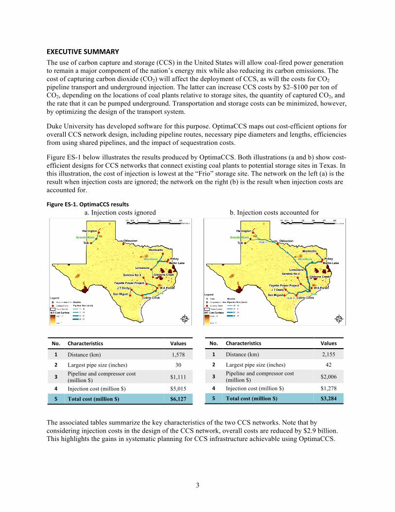
Figure ES-1 below illustrates the results produced by OptimaCCS. Both illustrations (a and b) show cost-efficient designs for CCS networks that connect existing coal plants to potential storage sites in Texas. In this illustration, the cost of injection is lowest at the “Frio” storage site. The network on the left (a) is the result when injection costs are ignored; the network on the right (b) is the result when injection costs are accounted for.
Figure ES-‐1. OptimaCCS results a. Injection costs ignored b. Injection costs accounted for
No. Characteristics Values
1 Distance (km) 1,578
2 Largest pipe size (inches) 30
3 Pipeline and compressor cost (million $) $1,111
4 Injection cost (million $) $5,015
5 Total cost (million $) $6,127
No. Characteristics Values
1 Distance (km) 2,155
2 Largest pipe size (inches) 42
3 Pipeline and compressor cost (million $) $2,006
4 Injection cost (million $) $1,278
5 Total cost (million $) $3,284
The associated tables summarize the key characteristics of the two CCS networks. Note that by considering injection costs in the design of the CCS network, overall costs are reduced by $2.9 billion. This highlights the gains in systematic planning for CCS infrastructure achievable using OptimaCCS.
4
1. INTRODUCTION Coal-fired power is a major component of the nation’s energy mix and projections suggest it will be for decades to come (U.S. Energy Information Administration 2011). If so, addressing climate change will require the deployment of technologies to capture and store carbon dioxide (CO2) emissions. Collectively, these technologies are referred to as carbon capture and storage (CCS).
A CCS system consists of three major elements:
• technology to capture emissions at industrial sites and power plants; • a pipeline network to transport carbon from the source to the storage sites; and • geologic sinks to store carbon safely.
A major hurdle to the deployment of CCS is its high cost. The cost of capturing carbon depends on a number of factors, including how the plant generates power, what type of fuel is used, the plant’s capacity, the capture technology implemented, and how much CO2 is captured. Transportation and injection costs are highly variable and are determined by the spatial arrangement of the plants, the quantity of CO2 to be transported, the location of sequestration sites, injection costs at these sites, and the level of cooperation among power plant operators.
A comprehensive design for a system—one that it is optimized based on all of the major factors that affect a CCS system—can significantly reduce the overall cost of the system (Middleton and Bielicki 2009). The Nicholas Institute for Environmental Policy Solutions and Nicholas School of the Environment at Duke University have developed a spatial economic model, OptimaCCS, which minimizes CCS pipeline construction and injection costs by considering
• the most cost-effective CCS pipeline network design for transporting and injecting CO2; • site-specific costs associated with CO2 transportation and injection; • possible cost reductions from collaboration on pipeline construction by power plant operators;
and • the relationships between site-specific injection costs and the resultant CCS infrastructure.
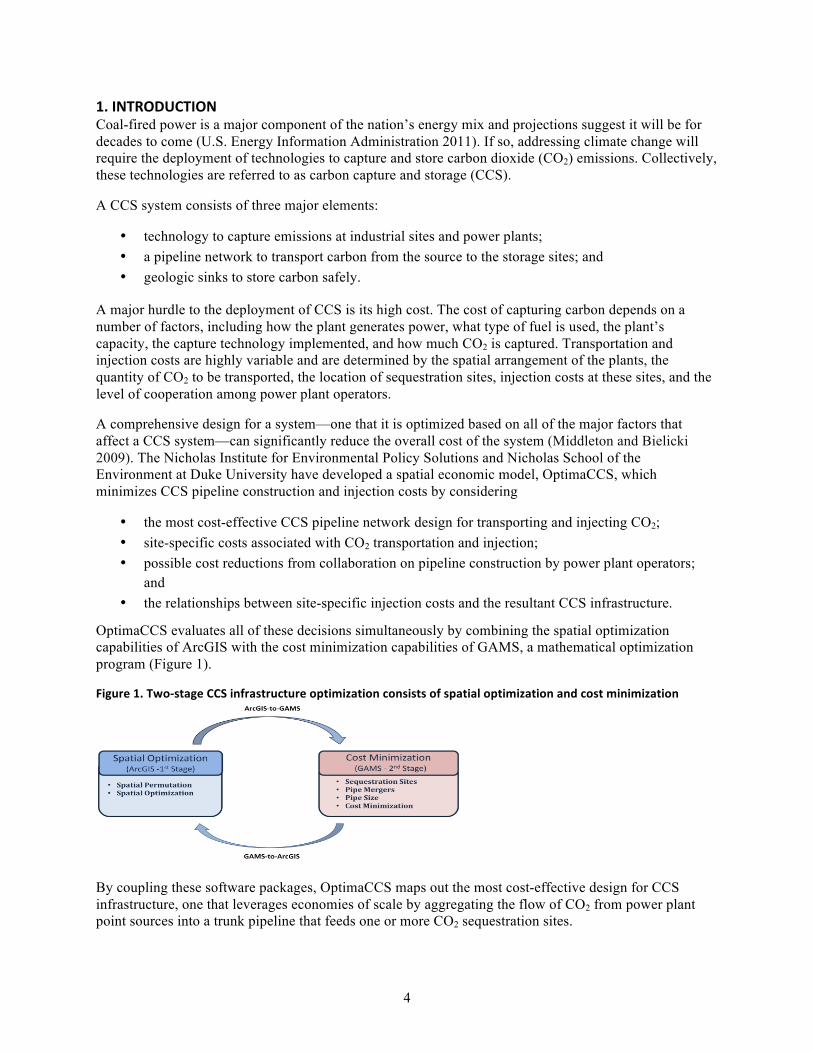
OptimaCCS evaluates all of these decisions simultaneously by combining the spatial optimization capabilities of ArcGIS with the cost minimization capabilities of GAMS, a mathematical optimization program (Figure 1).
Figure 1. Two-‐stage CCS infrastructure optimization consists of spatial optimization and cost minimization
By coupling these software packages, OptimaCCS maps out the most cost-effective design for CCS infrastructure, one that leverages economies of scale by aggregating the flow of CO2 from power plant point sources into a trunk pipeline that feeds one or more CO2 sequestration sites.
5
2. TEXAS EXAMPLE
2.1. Deployment scenarios We demonstrate OptimaCCS using a set of coal-fired power plants and candidate sequestration sites in Texas. We calculate the costs of two scenarios: one in which storage is ignored, and one in which storage is considered.
2.2. Power plants The power plants in this example have been selected using the Nicholas Institute’s version of the U.S. Energy Information Agency’s National Energy Modeling System, denoted as NI-NEMS. NI-NEMS identifies coal-fired power plants that would retrofit for carbon capture, based on an algorithm developed by the National Energy Technology Laboratory. This algorithm evaluates tradeoffs between retrofitting, retiring, and purchasing emission allowances. Here we include the type of bonus allowances proposed in Climate Change Bill H.R. 2454 (Waxman and Markey 2009) and the American Power Act (APA) (Kerry and Lieberman 2010) for plants that retrofit with CCS technology.
Using this framework for our analysis, we assume the federal government provides $95/ton1 of captured CO2, and that the initial price of CO2 is $20/ton starting in 2013. This price increases 5% annually, as assumed in the U.S. Environmental Protection Agency’s (EPA) analysis of the Waxman-Markey Climate Change Bill (U.S. Environmental Protection Agency 2009) and the American Power Act (U.S. Environmental Protection Agency 2010). Based on these assumptions, NI-NEMS identified 14 existing coal-fired power plants as potential retrofit candidates. These are listed Table 1, along with the amount of CO2 that would be captured at each plant.
Table 1. Coal-‐fired power plants in Texas identified by NI-‐NEMS as having CCS potential Plant name Operator County Capacity
(GW) Emissions
(Mt CO2/year) Captured
(Mt CO2/year)
Limestone NRG Energy Limestone 1.85 0.72 6.48
Harrington Xcel Energy Potter 1.08 0.30 2.66
Tolk Xcel Energy Lamb 1.14 0.38 3.41
Pirkey American Electric Power Harrison 0.72 0.51 4.56
Gibbons Creek Texas Municipal Power Agency
Grimes 0.45 0.37 3.35
J.T. Deely & Spruce CPS Energy Bexar 1.50 0.79 7.14
W.A. Parish NRG Energy Fort Bend 3.97 0.47 4.27
Monticello Luminant Energy Titus 1.98 0.66 5.93
Fayette Power Project
Lower Colorado River Authority
Fayette 1.69 0.16 1.48
San Miguel San Miguel Electric Coop Inc. Atascosa 0.41 0.17 1.52
Oklaunion American Electric Power Wilbarger 0.72 0.08 0.72
Martin Lake Luminant Energy Rusk 2.38 0.68 6.11
Sandow No. 4 Luminant Energy Milam 1.14 0.45 4.08
Coleto Creek International Power Goliad 0.60 0.57 5.09
Total 6.31 56.80
1 The term ton (abbreviated t) in this paper refers to the metric ton (1,000 kg). The abbreviation Mt refers to the megaton (1 million tons).
6
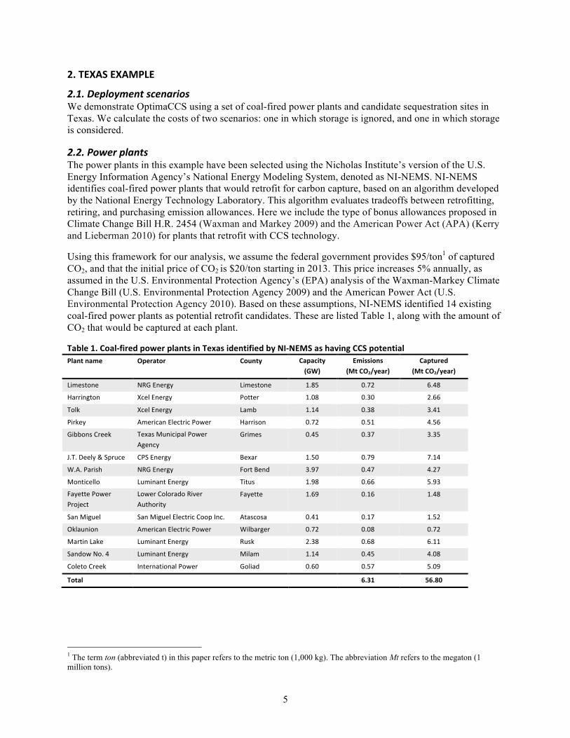
The locations of the plants are shown in Figure 2. Together, the plants have a combined capacity of 19.3 gigawatts (GW) and a potential for capture of 56.8 Mt CO2/yr.
Figure 2. Map of candidate power plants identified by NI-‐NEMS as well as three saline aquifers with significant storage potential
2.3. Saline aquifers Texas has three large-capacity deep saline formations for storing CO2: the Frio basin, the Woodbine basin, and the Granite Wash basin (Figure 3). Combined, the aquifers could store 350–1,400 billion t CO2/yr (National Energy Technology Laboratory 2010). In the reservoir characterization of these and nine other such saline aquifers, Eccles et al. (2009) arrived at the estimates for capacity, average injection rate, and average CO2 injection cost given in Table 2. Note that according to these estimates, the Frio’s average injection cost is six times lower than that of other basins.
Table 2. Average marginal CO2 injection cost estimate
Source: Eccles et al. 2009.
Saline Aquifers Avg marginal injection cost ($/ton)
Frio $0.75/ton
Granite Wash $4.50/ton
Woodbine $4.50/ton
7
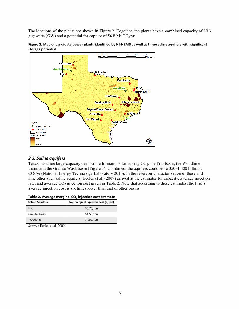
2.4. Cost surface A cost surface developed at Massachusetts Institute of Technology (MIT) (Herzog et al. 2007) is utilized to represent the relative cost of constructing a pipeline through various types of terrain by considering both the geographical features as well as social and political data (Figure 3). The cost surface is a raster layer of the continental United States with a cell size of 1 km2. The cell values are multipliers of an assumed baseline pipeline cost. This baseline pipeline cost (cost multiplier of 1) is for a pipeline that traverses a flat surface (without any obstacles) and includes the fixed cost of material, labor, and miscellaneous costs. The multiplier adjusts cost by factoring in the contribution of land slope, protected areas, and crossings of three line-‐type obstacles (waterways, railroads, and highways) (Herzog et al. 2007).
Figure 3. MIT's cost surface
3. RESULTS
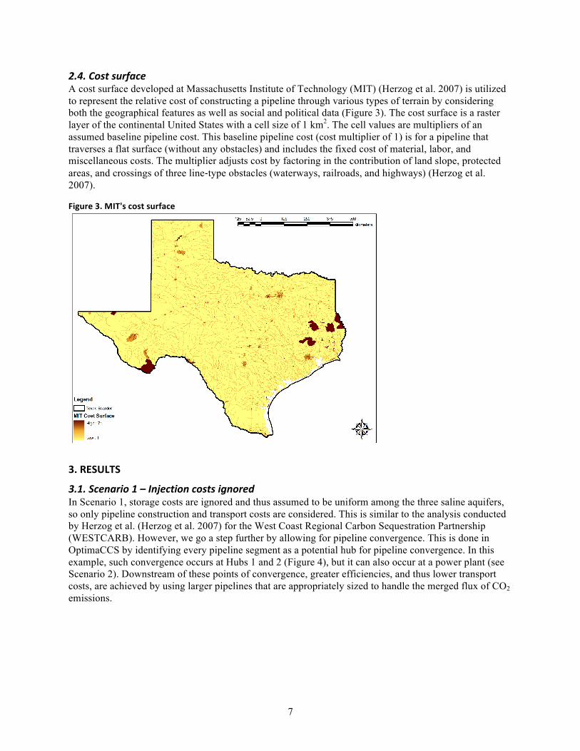
3.1. Scenario 1 – Injection costs ignored In Scenario 1, storage costs are ignored and thus assumed to be uniform among the three saline aquifers, so only pipeline construction and transport costs are considered. This is similar to the analysis conducted by Herzog et al. (Herzog et al. 2007) for the West Coast Regional Carbon Sequestration Partnership (WESTCARB). However, we go a step further by allowing for pipeline convergence. This is done in OptimaCCS by identifying every pipeline segment as a potential hub for pipeline convergence. In this example, such convergence occurs at Hubs 1 and 2 (Figure 4), but it can also occur at a power plant (see Scenario 2). Downstream of these points of convergence, greater efficiencies, and thus lower transport costs, are achieved by using larger pipelines that are appropriately sized to handle the merged flux of CO2 emissions.
8
Figure 4. Optimal pipeline network assuming uniform storage costs
Under Scenario 1, Optima CCS connects each of the 14 power plants to the closest sequestration site (Figure 4). This results in separate pipeline networks that feed each of the three saline aquifers. The Granite Wash pipeline network (Tolk, Harrington, and Oklaunion plants) has a construction cost of about $231.5 million, a total length of 474.7 km, and total CO2 delivery of 6.8 Mt CO2/yr (Figure 4). The Woodbine pipeline network (Monticello, Pirkey, Martin-Lake, Limestone, and Gibbons Creek plants) has a total construction cost of about $368.9 million, a length of 459.1 km, and a CO2 delivery of 26.4 Mt CO2/yr (Figure 4). The Frio pipeline network (Sandow No. 4, Fayette Power Project, W.A. Parish, J.K. Spruce, J.T. Deely, San Miguel, and Coleto Creek plants) has a construction cost of about $511.3 million, a length of 645.1 km, and a CO2 delivery of 23.6 Mt CO2/yr (Figure 4).
Table 3. Optimal network costs assuming uniform storage costs Characteristics Scenario 1
Distance (km) 1,578.2
Largest pipe size (inches) 30
Pipeline and compressor cost (million $) $1,111.7
Combined, the three networks’ 1,578 km of pipeline would cost $1.1 billion to construct (Table 3). Again, in this case, site-specific injection costs are not included.
3.2. Scenario 2 – Varying injection costs considered In Scenario 2, the estimated storage costs for the three saline aquifers (Table 3) are now considered. Consequently, OptimaCCS analyzes the design of CCS infrastructure to minimize pipeline and injection costs. The result is a single, statewide pipeline that feeds into one saline aquifer, the low-cost Frio (Figure 5).
9
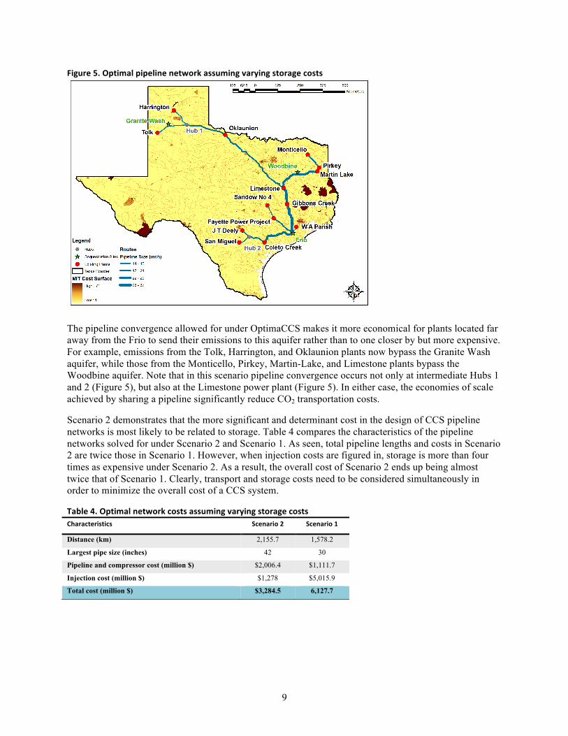
Figure 5. Optimal pipeline network assuming varying storage costs
The pipeline convergence allowed for under OptimaCCS makes it more economical for plants located far away from the Frio to send their emissions to this aquifer rather than to one closer by but more expensive. For example, emissions from the Tolk, Harrington, and Oklaunion plants now bypass the Granite Wash aquifer, while those from the Monticello, Pirkey, Martin-Lake, and Limestone plants bypass the Woodbine aquifer. Note that in this scenario pipeline convergence occurs not only at intermediate Hubs 1 and 2 (Figure 5), but also at the Limestone power plant (Figure 5). In either case, the economies of scale achieved by sharing a pipeline significantly reduce CO2 transportation costs.
Scenario 2 demonstrates that the more significant and determinant cost in the design of CCS pipeline networks is most likely to be related to storage. Table 4 compares the characteristics of the pipeline networks solved for under Scenario 2 and Scenario 1. As seen, total pipeline lengths and costs in Scenario 2 are twice those in Scenario 1. However, when injection costs are figured in, storage is more than four times as expensive under Scenario 2. As a result, the overall cost of Scenario 2 ends up being almost twice that of Scenario 1. Clearly, transport and storage costs need to be considered simultaneously in order to minimize the overall cost of a CCS system.
Table 4. Optimal network costs assuming varying storage costs Characteristics Scenario 2 Scenario 1
Distance (km) 2,155.7 1,578.2
Largest pipe size (inches) 42 30
Pipeline and compressor cost (million $) $2,006.4 $1,111.7
Injection cost (million $) $1,278 $5,015.9
Total cost (million $) $3,284.5 6,127.7
10
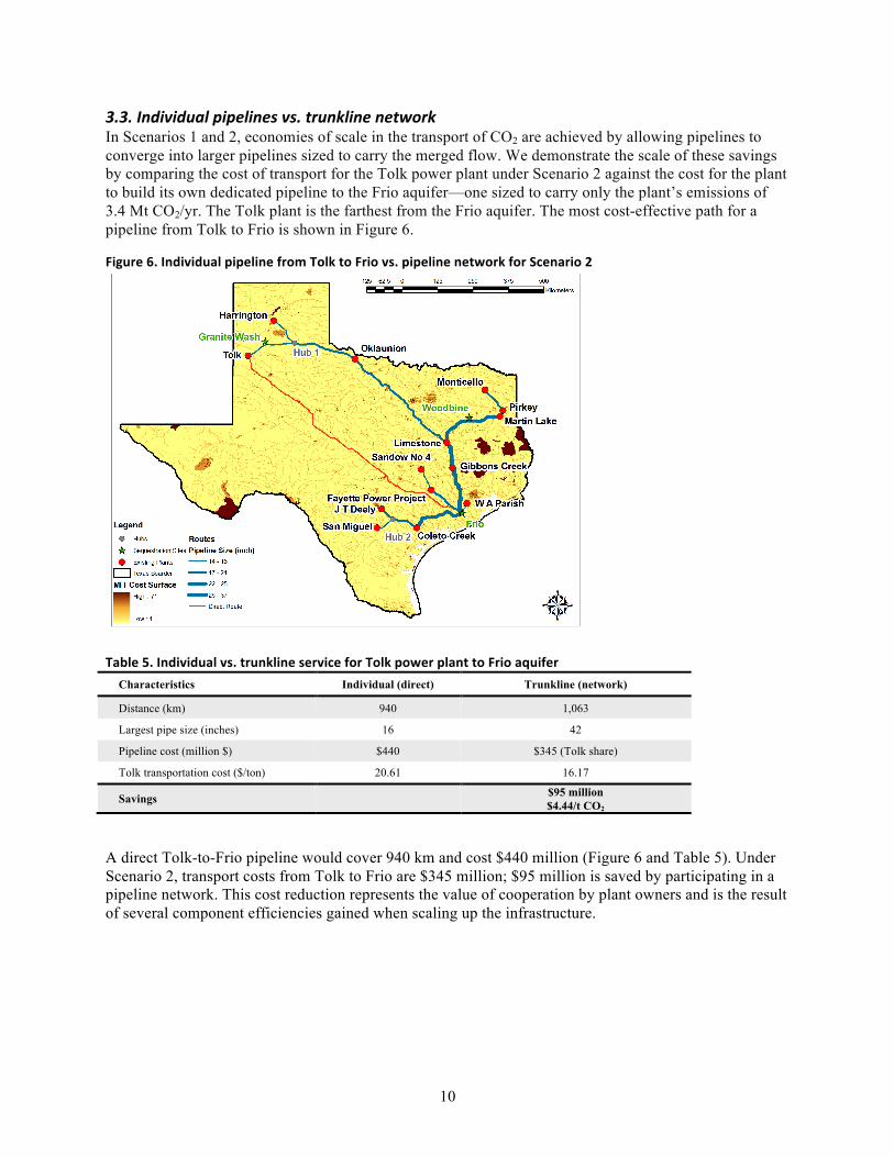
3.3. Individual pipelines vs. trunkline network In Scenarios 1 and 2, economies of scale in the transport of CO2 are achieved by allowing pipelines to converge into larger pipelines sized to carry the merged flow. We demonstrate the scale of these savings by comparing the cost of transport for the Tolk power plant under Scenario 2 against the cost for the plant to build its own dedicated pipeline to the Frio aquifer—one sized to carry only the plant’s emissions of 3.4 Mt CO2/yr. The Tolk plant is the farthest from the Frio aquifer. The most cost-effective path for a pipeline from Tolk to Frio is shown in Figure 6.
Figure 6. Individual pipeline from Tolk to Frio vs. pipeline network for Scenario 2
Table 5. Individual vs. trunkline service for Tolk power plant to Frio aquifer Characteristics Individual (direct) Trunkline (network)
Distance (km) 940 1,063
Largest pipe size (inches) 16 42
Pipeline cost (million $) $440 $345 (Tolk share)
Tolk transportation cost ($/ton) 20.61 16.17
Savings $95 million $4.44/t CO2
A direct Tolk-to-Frio pipeline would cover 940 km and cost $440 million (Figure 6 and Table 5). Under Scenario 2, transport costs from Tolk to Frio are $345 million; $95 million is saved by participating in a pipeline network. This cost reduction represents the value of cooperation by plant owners and is the result of several component efficiencies gained when scaling up the infrastructure.
11
4. CONCLUSION Through our Texas example, we show OptimaCCS can offer cost-effective designs for deploying CCS infrastructure under a range of spatial and economic constraints. Key points illustrated by this demonstration include:
• Significant CO2 transport savings can be achieved by networking multiple CO2 sources into a pipeline system rather than building individual pipelines from each power plant to storage sites.
• While transport costs are significant, injection costs over the lifetime of the CCS system are likely to be even more significant, and thus bear a greater influence on the design of a CO2 pipeline network, than the distances between CO2 sources and storage sites.
• The greatest cost savings are achieved when the design of the pipeline network considers both transport and storage constraints.
It is important to keep in mind that our illustration of OptimaCCS assumes all CCS infrastructure is deployed simultaneously, so these are best-case scenarios in terms of cost. Expenses will rise as infrastructure is deployed piecemeal over time. We are developing the ability to increment CO2 capture retrofits as they occur and to determine the correct sequence of segmented infrastructure expansions for economic efficiency.
Using the Texas example, comprehensive optimization yields a potential cost savings of roughly $3 billion and highlights the importance of systematic planning for CCS infrastructure at different levels of cooperation between CO2 sources and storage sites.
5. REFERENCES Eccles, J.K., L.F. Pratson, R.G. Newell, and R.B. and Jackson. 2009. “Physical and Economic Potential of
Geological CO2 Storage in Saline Aquifers.” Environmental Science and Technology 43(6): 1962–1969.
Herzog, H., W. Li, Z. Hongliang, M. Diao, G. Singleton, and M. Bohm. 2007. West Coast Regional Carbon Sequestration Partnership: Source - Sink Characterization and Geographic Information System - Based Matching. California Energy Commission, PIER Energy Related Environmental Research Program.
Herzog, H., W. Li, H. Zhang, M. Diao, G. Singleton, and M. Bohm. 2007. West Coast Regional Carbon Sequestration Partnership: Source Sink Characterization and Geographic Information System Based Matching. California Energy Commission, PIER Energy - Related Environmental Research Program.
Holtz, M.H., K. Fouad, P. Knox, S. Sakurai, and J. Yeh. 2005. Geologic Sequestration in Saline Formations, Frio Brine Storage Pilot Project, Gulf Coast Texas.
Kerry, J.F., and J.I. Lieberman. 2010. The American Power Act.
Middleton, R.S., and J.M. Bielicki. 2009. “A Scalable Infrastructure Model for Carbon Capture and Storage: SimCCS.” Energy Policy 37(3):1052–1060.
National Energy Technology Laboratory. 2010. 2010 Carbon Sequestration Atlas of the United States and Canada. Report of U.S. Department of Energy.
National Energy Technology Laboratory. 2008. Retrofitting Coal-Fired Power Plants for Carbon Dioxide Capture and Sequestration (CCS) - Exploratory Testing of NEMS for Integrated Assessments. National Energy Technology Laboratory. U.S. Department of Energy.

12
U.S. Energy Information Administration. 2011. Annual Energy Outlook 2011 with Projections to 2035. Washington, D.C.: U.S. Department of Energy/Energy Information Administration.
U.S. Environmental Protection Agency. 2010. EPA Analysis of the American Power Act in the 111th Congress. U.S. Environmental Protection Agency.
U.S. Environmental Protection Agency. 2009. EPA Preliminary Analysis of the Waxman-Markey Discussion Draft. U.S. Environmental Protection Agency.
Waxman, H.A., and J.E. Markey. 2009. The American Clean Energy and Security Act. 111th United States Congress.