OPTICS AND Optical Instrumentation

Optical imaging is the manipulation of light to elucidate the structures of objects

History of Optics Optical Instrumentation – light sources Optical Instrumentation – detectors Physical Optics Optical Instrumentation – intermediate optics

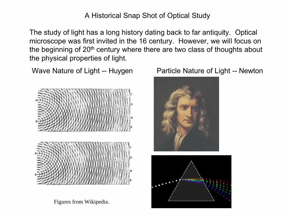
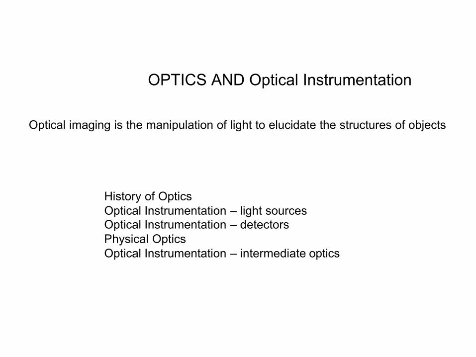
A Historical Snap Shot of Optical Study

The study of light has a long history dating back to far antiquity. Optical microscope was first invited in the 16 century. However, we will focus on the beginning of 20th century where there are two class of thoughts about the physical properties of light.

Wave Nature of Light -- Huygen Particle Nature of Light -- Newton

Figures from Wikipedia.

History of Optical Studies

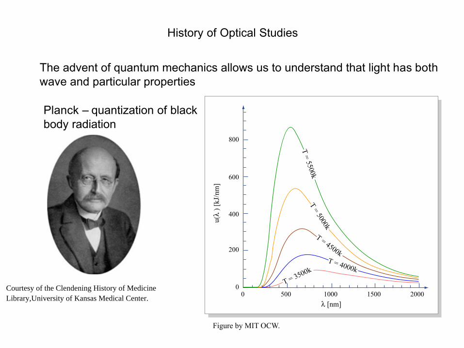
The advent of quantum mechanics allows us to understand that light has both wave and particular properties

Planck – quantization of black body radiation

Courtesy of the Clendening History of MedicineLibrary,University of Kansas Medical Center. 0

0500 1000 1500 2000

200

400

600

800

T = 5500kT = 5000k

T = 4500kT = 4000k

T = 3500k

λ [nm]

u(λ

) [kJ

/nm

]

Figure by MIT OCW.

History of Optical Studies

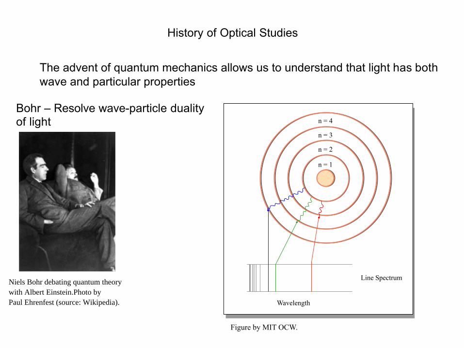
The advent of quantum mechanics allows us to understand that light has both wave and particular properties

Bohr – Resolve wave-particle duality of light

Niels Bohr debating quantum theorywith Albert Einstein.Photo byPaul Ehrenfest (source: Wikipedia).

n = 4

n = 3

n = 2

n = 1

Line Spectrum

Wavelength

Figure by MIT OCW.

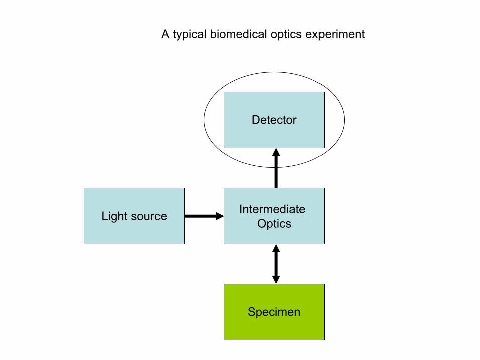
A typical biomedical optics experiment

Light source

Detector

Intermediate Optics

Specimen

Physical Principle of High Sensitivity Optical Detectors

High sensitivity photodetectors today are mainly based on two physical processes:

(1) Photoelectric effect

(2) Photovoltic effect

One can detect light by other processes such as heating. Power meter for laser light is called a thermopile and is based on heating by light – not very sensitive

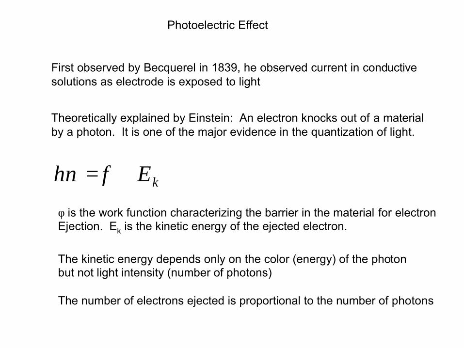
Photoelectric Effect

First observed by Becquerel in 1839, he observed current in conductive solutions as electrode is exposed to light

Theoretically explained by Einstein: An electron knocks out of a material by a photon. It is one of the major evidence in the quantization of light.

hn = f + Ek

f is the work function characterizing the barrier in the material for electron Ejection. Ek is the kinetic energy of the ejected electron.

The kinetic energy depends only on the color (energy) of the photon but not light intensity (number of photons)

The number of electrons ejected is proportional to the number of photons

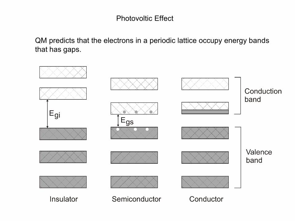
Photovoltic Effect

QM predicts that the electrons in a periodic lattice occupy energy bands that has gaps.

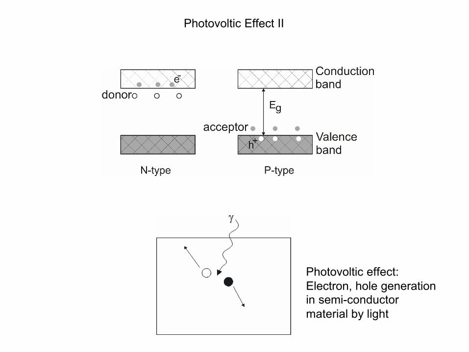
Photovoltic Effect II

Photovoltic effect: Electron, hole generation in semi-conductor material by light

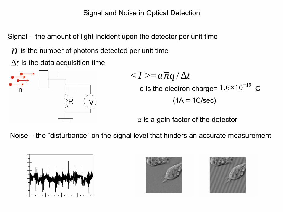
Signal and Noise in Optical Detection

Signal – the amount of light incident upon the detector per unit time

n is the number of photons detected per unit time

Dt is the data acquisition time

< I >= anq / Dt -

q is the electron charge= 1.6·10 19 C

(1A = 1C/sec)

a is a gain factor of the detector

Noise – the “disturbance” on the signal level that hinders an accurate measurement

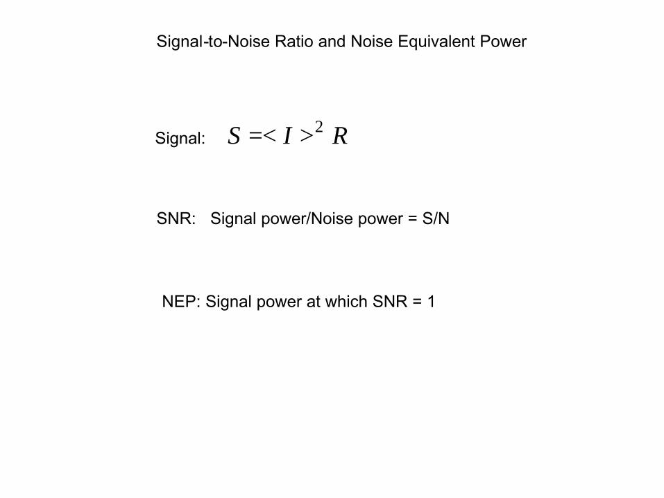
Signal-to-Noise Ratio and Noise Equivalent Power

Signal: S =< I >2 R

SNR: Signal power/Noise power = S/N

NEP: Signal power at which SNR = 1

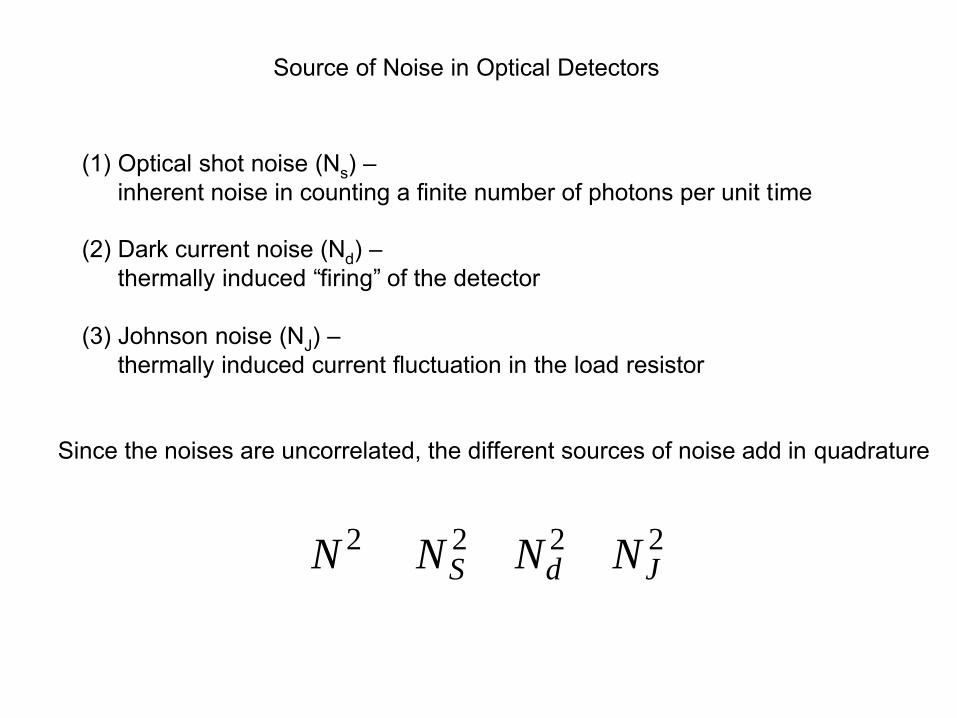
Source of Noise in Optical Detectors

(1) Optical shot noise (Ns) –inherent noise in counting a finite number of photons per unit time

(2) Dark current noise (Nd) –thermally induced “firing” of the detector

(3) Johnson noise (NJ) –thermally induced current fluctuation in the load resistor

Since the noises are uncorrelated, the different sources of noise add in quadrature

N 2 � NS 2 + Nd

2 + NJ 2

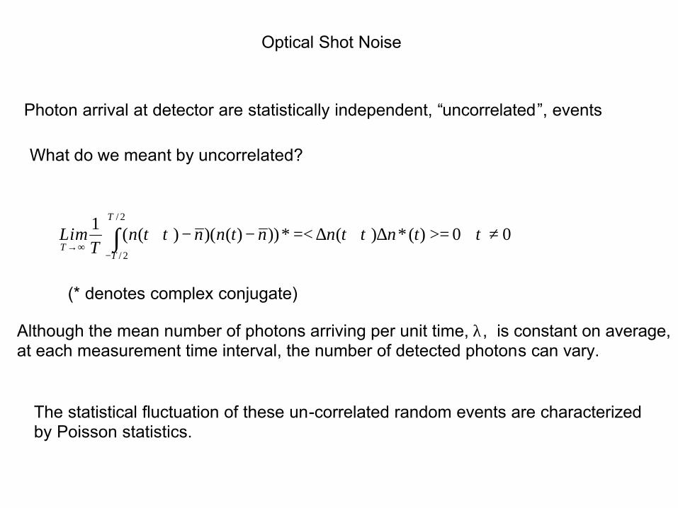
Optical Shot Noise

Photon arrival at detector are statistically independent, “uncorrelated”, events

What do we meant by uncorrelated?

1 T / 2

Lim � (n(t +t ) - n)(n(t) - n))* =< Dn(t +t )Dn*(t) >= 0 t „ 0 T fi¥ T -T / 2

(* denotes complex conjugate)

Although the mean number of photons arriving per unit time, l, is constant on average, at each measurement time interval, the number of detected photons can vary.

The statistical fluctuation of these un-correlated random events are characterized by Poisson statistics.

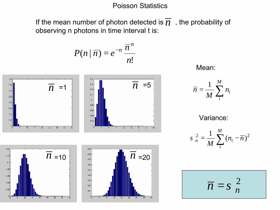
Poisson Statistics

If the mean number of photon detected is n , the probability of observing n photons in time interval t is:

n -nP(n | n) = e

n n!

Mean:

=1 =5

=10 =20

n n

n n

1 M

n = � niM i

Variance:

1 M

s n 2 = �(ni - n )2

M i

2 nn s=

Spectrum of Possion Noise I

¥

D ~ I ( f ) = � DI (t)e -i2pft dt where DI (t) = qDf (n(t) - n)

-¥

Assume photon number is Poisson distributed

Power spectral density: P ~( f ) = RDfDI

~*( f )DI ~( f )

Noise power: N ~( f , Df ) = P

~( f )Df

The power spectral density can be evaluated in a slightly round about way by considering the autocorrelation function:

¥

Autocorrelation function: g (t ) = RDf �DI (t +t )DI (t)*dt -¥

Because the event of Poisson process is completely independent of each other

g(t ) = Rs I 2d (t ) / Df

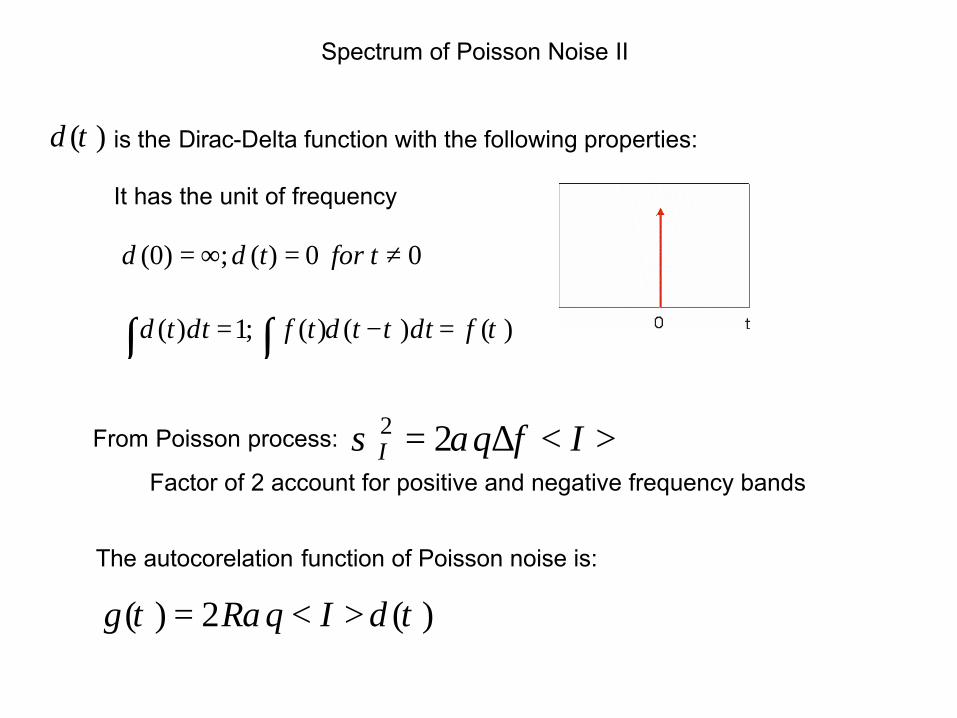
Spectrum of Poisson Noise II

d (t ) is the Dirac-Delta function with the following properties:

It has the unit of frequency

d (0) = ¥; d (t) = 0 for t „ 0

�d (t)dt =1; � f (t)d (t -t )dt = f (t )

From Poisson process: s I 2 = 2aqDf < I >

Factor of 2 account for positive and negative frequency bands

The autocorelation function of Poisson noise is:

g(t ) = 2Raq < I > d (t )

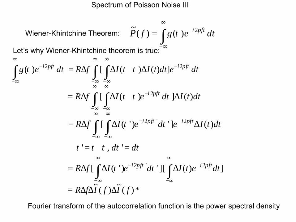
Spectrum of Poisson Noise III

¥

Wiener-Khintchine Theorem: P ~( f ) = � g(t )e -i2pft dt

-¥Let’s why Wiener-Khintchine theorem is true: ¥ ¥ ¥

g(t )e -i2pft dt = RDf [ DI (t +t )DI (t)dt]e -i2pft dt� � � -¥ -¥ -¥

¥ ¥

� � -i 2pft= RDf [ DI (t +t )e dt ]DI (t)dt -¥ -¥ ¥ ¥

= RDf [ DI (t ' )e -i2pft ' dt ' ]e+i2pftDI (t)dt� � -¥ -¥

t ' = t +t , dt ' = dt ¥ ¥

= RDf [ �DI (t ' )e -i 2pft ' dt '][ �DI (t)e+i 2pftdt] -¥ -¥

= RDfD ~ I ( f )DI ~( f )*

Fourier transform of the autocorrelation function is the power spectral density

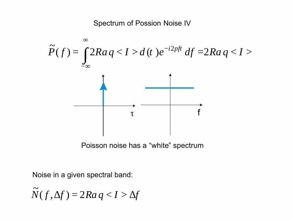
Spectrum of Possion Noise IV

¥

P ~( f ) = � 2Raq < I > d (t )e -i2pft df =2Raq < I >

-¥

ft

Poisson noise has a “white” spectrum

Noise in a given spectral band:

~ N( f ,Df ) = 2Raq < I > Df

Photon Shot Noise

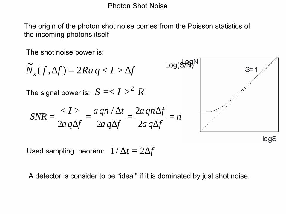
The origin of the photon shot noise comes from the Poisson statistics of the incoming photons itself

The shot noise power is:

N~ s ( f , Df ) = 2Raq < I > Df Log(S/N)

The signal power is: S =< I >2 R

< I > aqn / Dt 2aqnDfSNR = = = = n

2aqDf 2aqDf 2aqDf

Used sampling theorem: 1/ Dt = 2Df

A detector is consider to be “ideal” if it is dominated by just shot noise.