arX

iv:a

stro

-ph/

9610

211v

1 2

5 O

ct 1

996

Optical Observations of GRO J1655-40 in Quiescence I: A Precise

Mass for the Black Hole Primary

Jerome A. Orosz1,2 and Charles D. Bailyn1,3

Department of Astronomy, Yale University, P. O. Box 208101, New Haven, CT 06520-8101

E-Mail: orosz@astro.yale.edu, bailyn@astro.yale.edu

ABSTRACT

We report photometric and spectroscopic observations of the black hole binary GROJ1655-40 in complete quiescence. In contrast to the 1995 photometry, the light curvesfrom 1996 are almost completely dominated by ellipsoidal modulations from the sec-ondary star. Model fits to the light curves, which take into account the temperatureprofile of the accretion disk and eclipse effects, yield an inclination of i = 69.50±0.08 degand a mass ratio of Q = M1/M2 = 2.99 ± 0.08. The precision of our determina-tions of i and Q allow us to determine the black hole mass to an accuracy of ≈ 4%(M1 = 7.02 ± 0.22M⊙). The secondary star’s mass is M2 = 2.34 ± 0.12M⊙. The po-sition of the secondary on the Hertzsprung-Russell diagram is consistent with that of a≈ 2.3M⊙ star which has evolved off the main sequence and is halfway to the start of thegiant branch. Using the new spectra we present an improved value of the spectroscopicperiod (P = 2.d62157±0.d00015), radial velocity semiamplitude (K = 228.2±2.2 km s−1),and mass function (f(M) = 3.24 ± 0.09M⊙). Based on the new spectra of the sourceand spectra of several MK spectral type standards, we classify the secondary star asF3IV to F6IV. Evolutionary models suggest an average mass transfer rate for such asystem of M2 = 3.4× 10−9M⊙ yr−1 = 2.16× 1017 g s−1, which is much larger than theaverage mass transfer rates implied in the other six transient black hole systems, butstill barely below the critical mass transfer rate required for stability.

Subject headings: binaries: spectroscopic — black hole physics — X-rays: stars — stars:individual (GRO J1655-40)

1Visiting Astronomer at Cerro Tololo Inter-American Observatory (CTIO), which is operated by the Association of Universities forResearch in Astronomy Inc., under contract with the National Science Foundation.

2Present Address: Department of Astronomy & Astrophysics, The Pennsylvania State University, 525 Davey Laboratory, UniversityPark, PA 16802

3National Young Investigator

1

1. Introduction

A new bright X-ray source (designated GRO J1655-40) was discovered July 27, 1994 with the Burstand Transient Source Experiment (BATSE) on boardthe Compton Gamma Ray Observatory (Zhang et al.1994). The optical counterpart and the radio coun-terpart were identified soon after the announcementof the discovery by the BATSE team (Bailyn et al.1995a; Campbell-Wilson & Hunstead 1994). Aboutthree weeks after the initial hard X-ray outburst, ra-dio jets with apparent superluminal velocities wereobserved emerging from the source (Tingay et al.1995; Hjellming & Rupen 1995), making GRO J1655-40 only the second source in our Galaxy observed tohave superluminal jets and the first one to be opticallyidentified.

Bailyn et al. (1995b) established the spectroscopicperiod (2.d601± 0.d027) and the mass function (3.16±0.15M⊙) of the system using spectroscopic observa-tions made during late April and early May, 1995.The photometric observations by Bailyn et al. (1995b)from early 1995 showed that GRO J1655-40 is aneclipsing binary. The light curves from March andApril, 1995 all have deep triangular-shaped min-ima near the spectroscopic phase 0.75 (caused by aneclipse of the disk by the star) and much shallowerminima near the spectroscopic phase 0.25 (caused byan eclipse of the star by the disk). These observationsconfirmed earlier hints that GRO J1655-40 might bean eclipsing binary: Bailyn et al. (1995a) observeda single eclipse-like event in the photometry on thenight of August 17, 1994, and the model of the kine-matics of the radio jets proposed by Hjellming & Ru-pen (1995) gives an inclination of i = 85 deg. In spiteof the observations of optical eclipses, there has notyet been an unambiguous observation of an X-rayeclipse (e.g. Harmon et al. 1995a). The lack of X-ray eclipses and the presence of optical eclipses putsa tight constraint on the inclination of the orbit.

Unlike most “X-ray novae,” GRO J1655-40 contin-ued to have major outburst events in hard X-rays longafter its initial high-energy outburst (see Harmon etal. 1995a). There was an outburst event late March,1995 (Wilson et al. 1995) and another one startinglate July, 1995 (Harmon et al. 1995b). Not surpris-ingly, the V magnitude of the source during 1995 wastypically around V ≈ 16.5 (e.g. Bailyn et al. 1995b),somewhat higher than the quiescent value of V ≈ 17.3(Bailyn et al. 1995a). Furthermore, the shapes of the

light curves from 1995 are complicated. There arenight-to-night brightness variations, and the phases ofsome of the optical minima are not aligned preciselywith the spectroscopic phase (Bailyn et al. 1995b).X-ray heating and hot spots on an asymmetric accre-tion disk probably play a large role in explaining thecomplex light curves.

After the July/August, 1995 hard X-ray outburst,the source finally settled into true X-ray quiescence.From the period of late August, 1995 to late April,1996, the source was not detected by BATSE (Robin-son et al. 1996). The ASCA X-ray satellite madeseveral pointed observations in late March, 1996 aspart of a large multi-wavelength observing program(Robinson et al. 1996). The soft X-ray luminosity wasfound to be quite low, with Lx ≈ 2 × 1032 ergs s−1

(assuming a distance of d = 3.2 kpc—see Robinson etal. 1996), which is about a factor of 900 times smaller

than the optical luminosity of the secondary star(L2 ≈ 47L⊙, see Section 6). The extended periodof X-ray quiescence ended late April, 1996 when theall sky monitor on the Rossi X-ray Timing Explorer

satellite detected a sharp increase in brightness in thesoft X-rays (Remillard et al. 1996a). The source alsobrightened significantly in the optical and UV (Horneet al. 1996), and in the radio wavelengths (Hunstead& Campbell-Wilson 1996; Hjellming & Rupen 1996).

We have obtained additional photometry and spec-troscopy of GRO J1655-40 February and March, 1996.Much of the March data was taken as part of thelarger multi-wavelength program (Robinson et al.1996). These data show that the mean V magnitudeis consistent with its pre-outburst value and that inthe optical the system is dominated by light from thesecondary star. Since the accretion disk contributesa small fraction of the light and since GRO J1655-40eclipses, we have a unique opportunity to model thelight curves and obtain a reliable measure of the or-bital inclination, thereby leading for the first time areliable mass for a black hole. In Section 2 we describeour quiescent photometric observations. We presentan improved spectroscopic ephemeris in Section 3. InSection 4 we discuss the spectral classification of thesecondary star. In Section 5 we describe models of thelight curves. Section 6 is the discussion section detail-ing the evolutionary status of the secondary star, theinclination of the radio jet, and the stability of theaccretion. A short summary of the paper is presentedin Section 7. We have also included an Appendix tothis paper which gives a detailed description of the

2

Table 1

Journal of Spectroscopic Observations

1995 April 30-May 4a,b 1996 February 24-25c

Telescope CTIO 4.0 m CTIO 1.5 mDetector Loral 3072× 1024 Loral 1200× 800Grating KPGL #3 (527ℓ/mm) KPGL #3 (527ℓ/mm)Resolution 3.3 A (FWHM) 4.0 A (FWHM)Wavelength Coverage 3850-7149 A 4673-6657 ANumber of Spectra 73 12

aPreviously published in Bailyn et al. 1995b.

bThe heliocentric Julian date (HJD) range: 2 449 837.580 to 2 449 841.915

cHJD range: 2 450 137.792 to 2 450 138.890

code used to model the light curves.

2. Observations and Reductions

The spectroscopic observations from April andMay, 1995 published in Bailyn et al. (1995b) are sum-marized in Table 1. Additional spectra were taken inphotometric conditions February 24-25, 1996 with theRC spectrograph on the CTIO 1.5 meter telescope.The KPGL #3 grating and the Loral 1200×800 CCDcombination gave a dispersion of 1.68 A per pixel. AHe-Ar lamp was observed repeatedly to give the wave-length calibrations. In addition to the 12 spectra ofGRO J1655-40, we also obtained the spectra of 45different stars (most with two or more observations),including several radial velocity standards, flux stan-dards, and MK spectral type standards (Morgan &Kennan 1973).

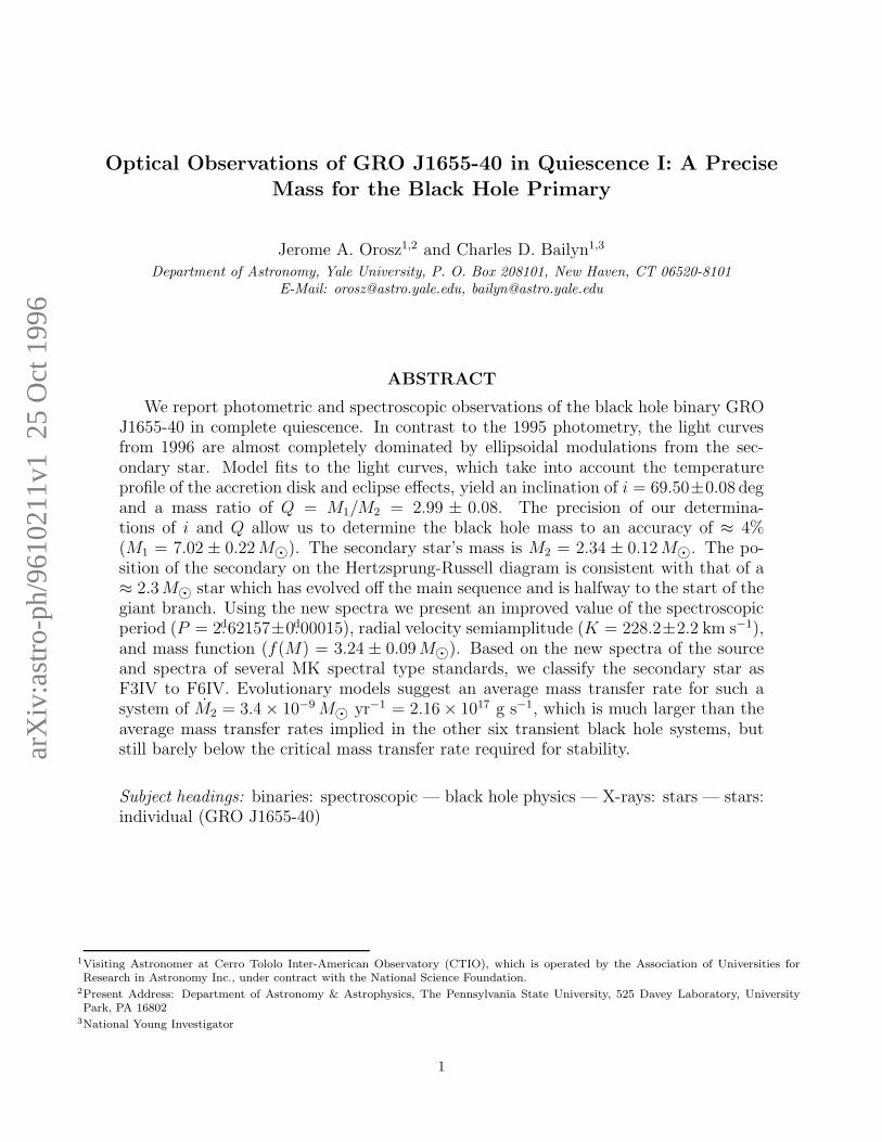
Photometry of the source was obtained February,March, and April, 1996 with the CTIO 0.9 metertelescope and Tek 2048 × 2046 #3 CCD (see Table2). All of the nights in February, 1996 were photo-metric and about half of the nights in the March-April, 1996 run were photometric. Standard IRAFtasks were used to process the images to remove theelectronic bias and to perform flatfielding corrections.The programs DAOPHOT IIe and DAOMASTER(Stetson 1987; Stetson, Davis, & Crabtree 1991; Stet-son 1992a,b) were used to compute the photometrictime series of GRO J1655-40 and several field com-

parison stars. The errors in the instrumental mag-nitudes were estimated by computing the standarddeviations in the light curves of several stable fieldstars. The sizes of these errors were found to be inreasonable agreement with the errors reported by theDAOMASTER program. We have adopted the errorsgiven by DAOMASTER in the analysis presented be-low. The instrumental magnitudes were transformedto the standard system using previously calibratedfield stars (Bailyn et al. 1995a). All of the February,1996 frames were usable. Out of the all the framestaken in March and April, one frame in B, two framesin R, and one frame in I were not used in any of theanalysis because of cosmic ray hits on or very nearthe image of GRO J1655-40.

3. A Refined Spectroscopic Ephemeris

The 73 spectra from April 30-May 4, 1995 wererebinned to match the slightly larger dispersion andsmaller wavelength coverage of the 12 spectra from1996. The radial velocities of the 85 spectra werefound by computing the cross-correlations (Tonry &Davis 1979) against a spectrum of 40 Leo (=HD89449), a radial velocity standard star of spectral typeF6IV (radial velocity = +6.5± 0.5 km s−1) that wasobserved February, 1996. The cross-correlations werecomputed over the wavelength region between Hβ andHα, excluding the strong interstellar absorption lines(see Bailyn et al. 1995a) and regions corrupted by bad

3

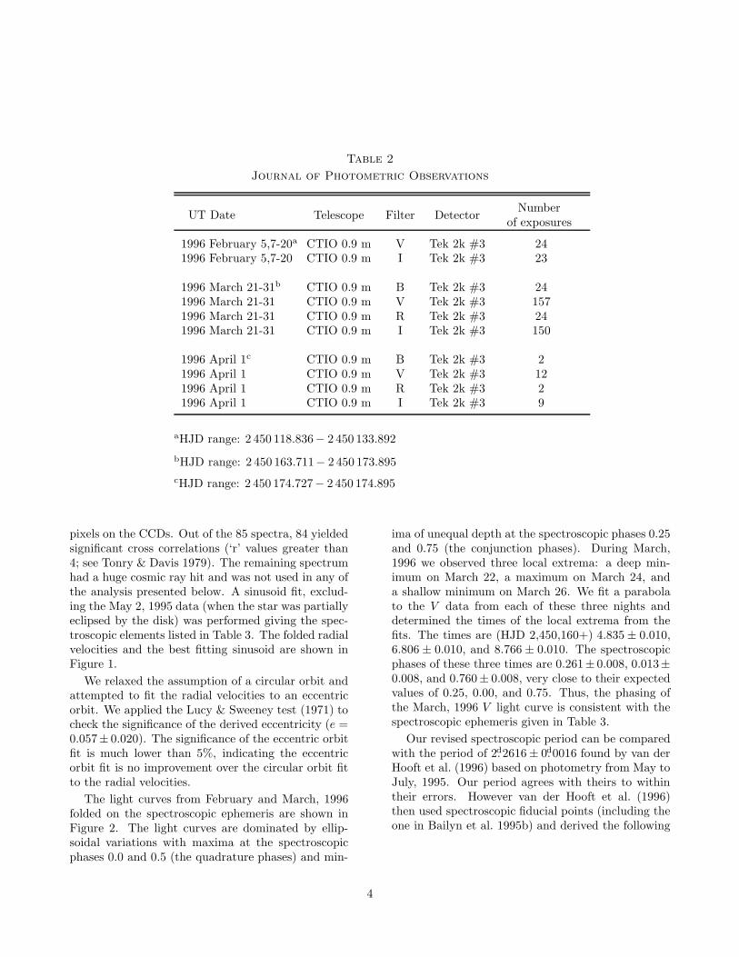
Table 2

Journal of Photometric Observations

UT Date Telescope Filter DetectorNumber

of exposures

1996 February 5,7-20a CTIO 0.9 m V Tek 2k #3 241996 February 5,7-20 CTIO 0.9 m I Tek 2k #3 23

1996 March 21-31b CTIO 0.9 m B Tek 2k #3 241996 March 21-31 CTIO 0.9 m V Tek 2k #3 1571996 March 21-31 CTIO 0.9 m R Tek 2k #3 241996 March 21-31 CTIO 0.9 m I Tek 2k #3 150

1996 April 1c CTIO 0.9 m B Tek 2k #3 21996 April 1 CTIO 0.9 m V Tek 2k #3 121996 April 1 CTIO 0.9 m R Tek 2k #3 21996 April 1 CTIO 0.9 m I Tek 2k #3 9

aHJD range: 2 450 118.836− 2 450 133.892

bHJD range: 2 450 163.711− 2 450 173.895

cHJD range: 2 450 174.727− 2 450 174.895

pixels on the CCDs. Out of the 85 spectra, 84 yieldedsignificant cross correlations (‘r’ values greater than4; see Tonry & Davis 1979). The remaining spectrumhad a huge cosmic ray hit and was not used in any ofthe analysis presented below. A sinusoid fit, exclud-ing the May 2, 1995 data (when the star was partiallyeclipsed by the disk) was performed giving the spec-troscopic elements listed in Table 3. The folded radialvelocities and the best fitting sinusoid are shown inFigure 1.

We relaxed the assumption of a circular orbit andattempted to fit the radial velocities to an eccentricorbit. We applied the Lucy & Sweeney test (1971) tocheck the significance of the derived eccentricity (e =0.057± 0.020). The significance of the eccentric orbitfit is much lower than 5%, indicating the eccentricorbit fit is no improvement over the circular orbit fitto the radial velocities.

The light curves from February and March, 1996folded on the spectroscopic ephemeris are shown inFigure 2. The light curves are dominated by ellip-soidal variations with maxima at the spectroscopicphases 0.0 and 0.5 (the quadrature phases) and min-

ima of unequal depth at the spectroscopic phases 0.25and 0.75 (the conjunction phases). During March,1996 we observed three local extrema: a deep min-imum on March 22, a maximum on March 24, anda shallow minimum on March 26. We fit a parabolato the V data from each of these three nights anddetermined the times of the local extrema from thefits. The times are (HJD 2,450,160+) 4.835± 0.010,6.806 ± 0.010, and 8.766 ± 0.010. The spectroscopicphases of these three times are 0.261± 0.008, 0.013±0.008, and 0.760± 0.008, very close to their expectedvalues of 0.25, 0.00, and 0.75. Thus, the phasing ofthe March, 1996 V light curve is consistent with thespectroscopic ephemeris given in Table 3.

Our revised spectroscopic period can be comparedwith the period of 2.d2616± 0.d0016 found by van derHooft et al. (1996) based on photometry from May toJuly, 1995. Our period agrees with theirs to withintheir errors. However van der Hooft et al. (1996)then used spectroscopic fiducial points (including theone in Bailyn et al. 1995b) and derived the following

4

Table 3

Orbital Parameters for GRO J1655-40

parameter result

Orbital period, spectroscopic (days) 2.62157± 0.00015K velocity (km s−1) 228.2± 2.2γ velocity (km s−1) −142.4± 1.6T0 (spectroscopic) (HJD 2 440000+) 9 839.0763± 0.0055Mass function (M⊙) 3.24± 0.09

Fig. 1.— The folded radial velocities of GRO J1655-40 and the best fitting sinusoid (see Table 3). Each point hasbeen plotted twice. Open diamonds indicate data from April 30, 1995; open triangles, filled stars, and open crossesindicate data from May 2, 3, and 4, 1995, respectively. The velocities from February 24, 1996 are indicated by thefilled triangles, and the filled circles indicate data from February 25, 1996. Parts of this figure appeared in Bailynet al. (1995b).

ephemeris:

Tmin(HJD) = 2 449 838.4279(30)+2.62032(50)N (1)

This period differs from our period by 2.5σ. Also, thephases of the three local extrema in our V light curvefrom March 1996 are by the above ephemeris 0.568±0.024, 0.320 ± 0.024, and 0.068 ± 0.024, significantlydifferent from their expected values of 0.50, 0.25, and0.00. Bailyn et al. (1995b) reported great difficultiesin phasing up their light curves fromMarch and April,1995—no single period could align all of the opticalminima with the radial velocities. It appears that thelight curves from May to July, 1995 still suffer fromphasing problems, although to a much smaller extentthan the earlier light curves from 1995. The period

derived solely from the radial velocities appears to bethe most reliable.

The refined period of P = 2.d62157± 0.d00015 rep-resents a great improvement in accuracy over the pre-vious value given in Bailyn et al. (1995b). Using thisnew period, we can now compute accurately the or-bital phase of observations made in 1994 and late1995. For example, Bailyn et al. (1995a) presentedphotometry from August 17, 1994 which showed evi-dence for an eclipse (the source got fainter and redderthen bluer and brighter over the 4.5 hours of observa-tions). Only one such eclipse-like event was observedin 1994. Using the refined orbital period, we findthat the spectroscopic phase of the time of minimum

5

Fig. 2.— The light curves from February, 1996 (left panels) and March, 1996 (right panels) folded on the spectro-scopic ephemeris (Table 3) are shown. Each point has been plotted for clarity. Error bars are shown for all of thepoints, but in many cases the size of the errors is smaller than the symbols.

6

Fig. 3.— The rms residuals of a polynomial fit to the difference spectrum as a function of the weight w for threedifferent template stars: an F3IV star (solid line), an F3V star (dotted line), and a G0V star (dashed line). In eachcase, the minimum of the curve can be accurately computed. The restframe spectrum was from 1996. See the textfor more details.

light (estimated to be at the heliocentric Julian date2,449,581.63) is 0.80. Curiously enough, the sharpoptical minimum observed April 2, 1995 (see Bailynet al. 1995b) also has a spectroscopic phase of 0.80(the phasing offsets of the light curves will be dis-cussed more below). The ASCA X-ray satellite ob-served GRO J1655-40 at the end of August 23, 1994(Inoue et al. 1994). During most of this observationthe X-ray flux stayed relatively low. Also, the X-rayspectrum from August 23 was quite different whencompared to subsequent observations, leading to thespeculation that an X-ray eclipse was observed (In-oue 1995, private communication). It turns out thatthe spectroscopic phases of the August 23 ASCA ob-servations are from 0.27 to 0.36—i.e. the star was be-hind the compact object. Thus some other mechanismmust be invoked to explain the X-ray light curve andspectrum from August 23, 1994.

4. Spectral Classification

During the April-May, 1995 observing run, thespectra of 33 different stars of spectral type F throughK and luminosity classes V through III were taken.During the February, 1996 run, we obtained the

spectra of 45 different stars, including nine Morgan-Keenan (1973) spectral type standard stars of classF. We used the technique outlined in Orosz et al.(1996) to classify the 1995 and 1996 spectra of GROJ1655-40. First, each continuum-normalized spec-trum of GRO J1655-40 is shifted to zero velocityand the lot of them are averaged together, creatinga “restframe” spectrum. To help minimize the ef-fects of an occasional cosmic ray, a “min-max” rejec-tion scheme was used where the lowest and highestvalues at each pixel were rejected before the averagewas computed. Then, the velocity shifts between thecomparison spectra and the restframe spectrum areremoved. Finally, the steps involved in the compar-ison are (1) each continuum-normalized and shiftedcomparison spectrum is scaled by a factor w (where0 ≤ w ≤ 1) and subtracted from the normalized rest-frame spectrum, (2) a low order polynomial is fit tothe difference spectrum, (3) the rms residuals of thefit (computed over the same region used to computethe cross-correlations) is recorded, and (4) steps (1)through (3) are repeated using different scaling fac-tors until the minimum rms is found, correspondingto the “smoothest” difference spectrum. In finding

7

Fig. 4.— The minimum rms (see the text) is plotted as a function of the spectral type of the template for the fourdifferent groups. The plotting symbol indicates the luminosity class of the template: open triangles for dwarfs,filled circles for subgiants, crosses for giants, and curved squares for supergiants. Templates that had a weightw > 1 are not shown (see the text). In each case, the lowest overall rms values occur for the spectral classes F3to F5. Note that many of the template stars had two or more observations, so that the total number of templatestars used is less than the number of symbols shown.

the rms of the fits to the difference spectra, we werecareful to avoid interstellar absorption lines and re-gions corrupted by bad columns on the CCDs. Fig-ure 3 shows a plot of the rms of the fit to the differ-ence spectrum as a function of the weight w for somerepresentative cases. In each case, the minimum ofthe curve can be determined accurately. All of theabove four steps are done on all of the comparisonspectra, and the comparison spectrum that has thelowest overall rms value is taken to be the spectrumwhose absorption lines most closely match those inthe restframe spectrum. The relative fluxes of therestframe spectrum and the difference spectrum givean estimate of the fraction of the total light due tothe accretion disk.

We have two restframe spectra of GRO J1655-40,one each from 1995 and 1996 (for the 1995 restframespectrum, we did not include the spectra from May2, 1995 because the star was partially eclipsed by thedisk). We also have two sets of template compari-son spectra from the same times. Every spectrum ineach set of templates was compared against both rest-

frame spectra. Since the 1995 spectra have a slightlyhigher spectral resolution than the 1996 spectra andsince the 1996 restframe spectrum has a lower signal-to-noise ratio than the 1995 restframe spectrum, agiven template spectrum will have a slightly higherminimum rms value when compared against the 1996restframe spectrum. We therefore grouped the com-parisons into four different cases: the 1995 templatespectra compared against the 1995 restframe spec-trum, the 1995 template spectra compared againstthe 1996 restframe spectrum, etc. The relative valuesof the minimum rms within each group can be usedto judge the best spectral match to the given rest-frame spectrum. Figure 4 shows the minimum rmsvalue plotted against the spectral type of the templatespectrum for the four different cases. In all four cases,there is a clear trend: the best matches for the GROJ1655-40 restframe spectra are the F3-F5 stars. Starswith spectral types later than F6 or earlier than F3provide much poorer matches to the restframe spec-tra. Based on the values of the weight w found forthe best matches, we conclude that the accretion disk

8

Fig. 5.— The restframe spectrum of GRO J1655-40 from February, 1996 (fourth from the top) and the spectra ofseveral F subgiants and giants. The anomalous strengths of the absorption lines near 5900 A and 6300 A in thespectrum of GRO J1655-40 are due to interstellar absorption. Each spectrum has been normalized to its continuumfit, and offsets have been applied for clarity.

contributed about 50% of the flux in V during Apriland May, 1995, and less than 10% of the flux in Vduring February, 1996.

This comparison technique is relatively sensitive tothe temperature class of the comparison star and rel-atively insensitive to the luminosity class of the com-parison star. We therefore cannot reliably determinethe luminosity class of the secondary star from thistechnique alone. However, in the case of GRO J1655-40, a main sequence F star is much too small to fillthe Roche lobe (Bailyn et al. 1995b), so the secondarystar must be somewhat evolved. Also, in the case ofthe 1996 restframe spectrum, many of the early Fdwarf template stars were excluded because a weightof w > 1 was required to get the minimum value ofthe rms. Hence, we are left with mainly subgiants andgiants. So, based on these other pieces of evidence,we conclude the secondary star in GRO J1655-40 is asubgiant, giving its full spectral classification as F3-F5 IV. Indeed, with the exception of the strong inter-stellar features, it is difficult to tell the difference be-tween the 1996 restframe spectrum of GRO J1655-40and the spectra of the nearby F subgiants and giants(see Figure 5).

The 1995 spectra of GRO J1655-40 were examinedin more detail to see if the best fitting spectral typedepends on the orbital phase. There was no indicationof any change in the spectral type as a function ofphase. Further details can be found in Orosz (1996).

5. Light Curve Models

The light curves shown in Figure 2 appear to bealmost completely ellipsoidal—there are two equalmaxima per orbit and two minima of unequal depthper orbit. The minimum at the spectroscopic phase0.25 (when the star is behind the compact object)is deeper because the gravity darkening near the L1

point is greater and hence the star appears darker (seeAvni 1978 and the Appendix). The symmetry andsmoothness of the GRO J1655-40 light curves from1996 are in strong contrast to the light curves for theother black hole binaries (e.g. McClintock & Remil-lard 1986; Wagner et al. 1992; Chevalier & Ilovaisky1993; Haswell et al. 1993; Haswell 1996; Remillard etal. 1996b; Orosz et al. 1996), where the light curvesare complicated by “flickering” about the mean lightcurve and by large asymmetries in the light curve thatslowly change with time (e.g. Haswell 1996).

9

Table 4

Input Model Parameters

parameter description comment

i inclination freeQ mass ratio (M1/M2 > 1) freerd outer radius of the diska freerinner inner radius of the diska fixed at 0.005Tdisk disk temperature at the outer edge freeξ power law exponent on disk

temperature radial distribution freeβrim flaring angle of the disk rim freeLx X-ray luminosity of the compact object fixed at 0.0W X-ray albedo fixed at 0.5Teff polar temperature of the secondary fixed at 6500 Kβ gravity darkening exponent fixed at 0.25u(λ) linearized limb darkening parameter fixedb

P orbital period fixed at 2.d62157f(M) mass function fixed at 3.24M⊙Ω ratio of rotational angular velocity

to orbital angular velocity fixed at 1.0f Roche lobe filling factor fixed at 1.0

aThe disk radii are scaled to the effective Roche lobe radius of the compactobject.

bLimb darkening parameters from Al-Namity (1978) and Wade & Rucin-ski (1985).

Because the light curves from February and March,1996 are smooth and symmetric and because the lu-minosity of the star dominates (i.e. the fraction of thelight from the disk is small, see Section 4), we havea unique opportunity to model the light curves andobtain a reliable constraint on the orbital inclination.We have developed a detailed code based on the workof Avni (Avni & Bahcall 1975; Avni 1978) to modelthe light curves, which is fully described in the Ap-pendix. The code uses full Roche geometry to accountfor the distorted secondary, and light from a circularaccretion disk is included. The code also handles mu-tual eclipses by the star and the disk. The effectsof X-ray heating on the secondary star are includedas well. There are several input model parameterswhich are summarized in Table 4. See the Appendixfor detailed discussions of these parameters and their

meaning.

For simplicity, we have fixed several of the inputparameters at reasonable values. For example, weknow the spectral type of the star (see the previoussection), from which we can get its effective temper-ature. The effective temperature of 6500 K is appro-priate for an F5 IV star (Straizys & Kuriliene 1981)and we will adopt the effective temperature of 6500K as the polar temperature. The gravity darkeningexponent is fixed at 0.25 since the star has a radia-tive envelope (see the Appendix). The limb darkeningcoefficient u(λ) is better determined from model at-mosphere computations, and we used values interpo-lated from tables given by Wade & Rucinski (1985).For fits to the 1996 light curves, we have fixed theX-ray luminosity at 0, based on the ASCA observa-tion in early 1996 that found Lx ≈ 2× 1032 ergs s−1,

10

Table 5

Fits to the March, 1996 photometry

parameter model 1 model 2a model 3

i (degrees) 69.50± 0.08 74.7± 1.2 69.54± 0.08Q 2.99± 0.08 3.3± 0.5 3.50± 0.08rd 0.747± 0.010 0.71± 0.01 0.748± 0.011Tdisk (K) 4317± 75 4525± 102 4429± 75βrim (degrees) 2.23± 0.18 1.54± 0.4 2.91± 0.18ξ −0.12± 0.01 −0.22± 0.01 −0.13± 0.01Lx 0.0 (fixed) 0.0 (fixed) 0.0 (fixed)W 0.5 (fixed) 0.5 (fixed) 0.5 (fixed)Teff (K) 6500 (fixed) 6500 (fixed) 7000 (fixed)χ2ν 1.1551 3.2391 1.1816

aNo checking for eclipses done.

almost three orders of magnitude lower than the op-tical luminosity of the secondary star (L2 ≈ 47L⊙,see the next Section). In the case where Lx = 0, theexact value of the X-ray albedo W is of course irrel-evant. For fits to the March 1995 light curves whereLx ≫ L2, we have adopted W = 0.5 (see the Ap-pendix), although other values of the X-ray albedoW have been used (for example van der Hooft et al.(1996) used W = 0.4). Since there is mass transfertaking place, we assume the star fully fills its Rochelobe and that it is in synchronous rotation.

For fits to the 1996 light curves, we are left withsix free parameters. The six free parameters in themodel are the inclination of the orbit (i), the massratio (Q ≡ M1/M2), the outer radius of the diskin terms of the primary’s effective Roche lobe ra-dius (rd), the temperature at the outer edge of thedisk (Tdisk), the flaring angle of the rim of the disk(βrim, where the thickness of the disk at the outeredge is given by 2rd tanβrim), and the power law ex-ponent on the disk’s radial temperature distribution(ξ, where the disk temperature varies with radius asT (r) = Tdisk(r/rd)

ξ).

We first fit models to the BV RI light curves fromMarch, 1996, as the phase coverage and spectral cov-erage from that time is the most complete. We foldedthe data on the photometric phase convention used inthe code where the photometric phase 0.0 corresponds

to the time the secondary is directly in front of thecompact object (i.e. T0(photo) = T0(spect) + 0.75P ).As discussed in Section 3, the phases of the threelocal extrema observed in March, 1996 are all latein phase by ≈ 0.011. We found that the model fitswere slightly better after a phase shift of 0.011 wasremoved from the folded curves. Since there are farfewer points in the B and R filters, we gave each pointin B and R seven times more weight when comput-ing the chi-square of the fit. This procedure resultedin equal weight being given to each filter. Figure 6shows the fits and the residuals and Table 5 lists themodel parameters (under “model 1”). Note that thedata in all four filters were fit simultaneously. Themodel fits the observed light curves from all four fil-ters quite well—the scatter in the residuals is typicallyless than 0.02 magnitudes. The 1σ statistical errorsfor each parameter were estimated using primarily aMonte Carlo “bootstrap” method (Press et al. 1992—see the Appendix). For this model, the accretion diskcontributes about 5% of the flux at 5500 A, consistentwith the measurement of ≤ 10% from late February,1996 (see the previous Section).

As a test of the accuracy of the 1σ errors derivedfrom the bootstrap analysis, we performed fits the theMarch 1996 light curves with the value of Q at fixedat several different input values. The other five pa-rameters were free and adjusted to find the minimum

11

Fig. 6.— The model fits to the B, V , R, and I light curves from March, 1996 (large panels) and the residuals ofthe fits (i.e. the data minus the model—small panels). Table 5 gives the model parameters under “model 1.”

12

Fig. 7.— Upper left: The value of the reduced chi-square as a function of the mass ratio Q, where the value of Q isfixed at each input value and the other five parameters are adjusted until the chi-square is minimized. Lower left:An expanded view of the χ2

ν vs. Q curve. The dotted lines indicate the change in the chi-square required for a 1,2, and 3σ change in a single parameter (i.e. ∆χ2 = 1, 4, and 9). Upper and lower right: similar to the left panels,but for fits with the inclination angle i fixed at various input values.

reduced chi-square at each input value of Q. The leftpanels of Figure 7 shows the χ2

ν vs. Q curve. Thedashed lines shown in the lower left panel of Figure7 indicate the change in χ2

ν representing a 1, 2, and3σ change in a single parameter (i.e. ∆χ = 1, 3, and9). A change in Q of 0.08 (the 1σ error derived froma Monte Carlo bootstrap analysis) in either directionfrom its value at the minimum causes the χ2

ν to in-crease by approximately the amount indicated by thelowest dashed line. The right panels of Figure 7 showthe equivalent computation done with the value of ifixed at several different values. Like before, a 1σchange in the parameter i (0.08) from the best valuecauses the value of χ2

ν to increase by approximatelythe amount indicated the lowest dashed line in thelower right panel. The χ2

ν v.s. i curve has a secondaryminimum at i = 67.7 deg and χ2

ν = 1.1620, which isgreater than the 2σ deviation from the primary min-imum at i = 69.5 deg and χ2

ν = 1.1551. While weare confident that the errors derived from the boot-strap analysis are a reasonable representation of thetrue internal statistical errors, there may be system-atic errors due to physical effects not included in themodel. Given how well the model fits the data, we

suspect that such systematic errors are likely to besmall. We are also confident that we have found theglobal minimum of χ2

ν since we have searched a largeamount of parameter space.

For each model with Q fixed at a given input value,there exists a value of the inclination i found from thebest fit. For the whole range of Q shown in the upperleft panel of Figure 7, the corresponding best valuesof i range from 68.40 ≤ i ≤ 71.1 deg. Likewise, forthe models with the inclination angle i fixed at sev-eral values (the upper right panel of Figure 7), thecorresponding best values of the mass ratio Q are inthe range 2.52 ≤ Q ≤ 4.23. Thus, the key geomet-rical parameters i and Q vary little and seem to bereasonably well determined. Based on the behavior ofχ2 near the minimum, we adopt the 1σ and 3σ rangesof the inclination i:

69.42 deg ≤ i ≤ 69.58 deg (1σ)

69.0 deg ≤ i ≤ 70.6 deg (3σ)

and the mass ratio Q:

2.91 ≤ Q ≤ 3.07 (1σ)

2.60 ≤ Q ≤ 3.45 (3σ).

13

Fig. 8.— The system as it appears projected onto the plane of the sky for the model parameters given in Table 5,model 1. The photometric phase is 0 deg for the bottom panel and 170 deg for the top panel.

14

The geometry of the system is shown schematicallyfor two different phases in Figure 8. Note that thecompact object is not eclipsed by the secondary star.We would therefore not expect to see X-ray eclipses(assuming the X-rays are emitted from a relativelysmall region centered on the compact object), and infact no X-ray eclipses have been seen (e.g. Harmon etal. 1995a). The star does block part of the disk (andvice-versa) at certain phases, so we expect to still seegrazing optical eclipses, the depths of which dependon the size of the disk and the relative brightnessesof each component. In order to assess how importantthe grazing eclipses are in determining the final overallshapes of the light curves, we performed a model fit tothe BV RI data from March, 1996 where the eclipsechecking routines were turned off. In this case themodel light curve is just the normal ellipsoidal lightcurve from a Roche lobe filling star plus a constantflux from the accretion disk (where the amount of disklight relative to the amount of star light in generaldepends on the filter bandpass). Table 5 gives thevalues of the parameters (under “model 2”). The fit ispoor, as one can deduce from the relatively large valueof the reduced chi-square (χ2

ν = 3.239, compared toχ2ν = 1.1551 for model 1). The fits are poor when

eclipses are not accounted for in the computations fortwo reasons: (i) the difference in the depths of thetwo minima in the model light curve are too small,and (ii) the dependence of the light curve amplitudewith color is not properly accounted for by the model(the amplitude of the observed light curve is largestin B and smallest in I, see Figure 2).

Our numerical experiments also show that the fi-nal fitted parameters do not depend strongly on theassumed secondary star parameters. For example, inthe case of a Roche lobe-filling star, the temperaturewill not be constant over the surface (see Equation(A3) of the Appendix). In particular, the side of thestar near the L1 point should be the coolest. Thetemperature of 6500 K corresponding to the observedspectral type therefore represents some kind of flux-weighted average of the temperatures over the sur-face, and technically not the star’s polar tempera-ture. However, our spectral coverage was not uni-form in phase and spectra used to determine the spec-tral type mainly came from phases near the quadra-ture phases. The temperatures corresponding to thebrightest parts of the projected stellar disk at thesephases are within ≈ 200 K of the polar temperature.Also, we could not detect any change in the spectral

type of the individual observations as a function ofphase (this includes the data from May 2, 1995 whenthe star was behind the disk and the L1 point wasin full view—see Orosz (1996)), which suggests otherfactors are at work when the observed spectrum ata given phase is produced. Thus, we believe we arenot making a large error when adopting the temper-ature derived from the observed spectral type as thepolar temperature. In this same vein, we fit a modelto the March, 1996 data where the polar tempera-ture of the secondary star was 7000 K, appropriatefor an F2 IV star (Straizys & Kuriliene 1981). Theresults for the geometrical parameters, given in Table5 under “model 3”, are quite similar to the resultsusing Teff = 6500 K (model 1). Finally, we comparedthe linearized limb darkening parameters u(λ) inter-polated from tables given by Al-Naimiy (1978) andWade & Rucinski (1985). The shapes of the u(λ)curves were very similar—the only large differencesoccurred for wavelengths blueward of the B band. Asa result, the fits to the BV RI light curves of GROJ1655-40 were similar when the limb darkening coef-ficients were used from either source.

The stellar evolution models (see the Discussion)indicate the secondary has a radiative envelope. Wehave therefore adopted a gravity darkening exponentof β = 0.25. We tried a model fit to the light curveswith the gravity darkening exponent set to β = 0.08,the value appropriate for stars with convective en-velopes (Lucy 1967). The model fits were much worsein this case (we could not find a fit with χ2

ν < 2).When β = 0.08, the temperature contrast over thestar is smaller (see Equation (A3) of the Appendix),leading directly to a smaller brightness contrast, es-pecially between the side of the star near the L1 pointand the opposite side. Since the brightness contrastbetween the side facing the compact object and theopposite side is greatly reduced, the inclination needsto be higher to produce the same observed ampli-tude of the light curves. However, as the inclinationgrows closer to 90 deg, the eclipses become deeper andthe fine balance between the primary and secondaryeclipse depths is disturbed, making the simultaneous

fits to all four colors much more difficult. Thus, basedboth on the stellar evolution models and the qualityof the fits, we conclude that the gravity darkeningexponent of β = 0.25, appropriate for a star with aradiative envelope, is the correct choice.

As one can see from Figure 2, the shapes of theFebruary, 1996 light curves are almost identical to

15

Fig. 9.— The two panels show the February, 1996 data minus the March, 1996 model (Table 5, model 1).

the shapes of the light curves from March, 1996. Theonly noticeable difference between the two curves oc-curs near the minimum at the photometric phase 0.5(which is the spectroscopic phase 0.25): that mini-mum in the February light curves is slightly deeperthan that minimum in the March light curves. Notsurprisingly, models that fit the March, 1996 data areconsistent with the February, 1996 data (Figure 9):the residuals in the V band have a mean of 0.009 anda standard deviation of 0.019 and the residuals in theI band have a mean of 0.013 and a standard deviationof 0.013. The only deviant points in the two filters arethose near the photometric phase 0.5 which are about0.05 magnitudes fainter than the model that fits thedata from March.

The light curves of GRO J1655-40 from March andApril, 1995 (see Bailyn et al. 1995b) look quite differ-ent from the light curves from 1996 (Figure 2). Firstof all, the source was about 0.7 to 0.8 magnitudesbrighter in V during early 1995 than it was duringearly 1996, probably a direct result of the fact thatthere was still considerable hard X-ray activity tak-ing place during that time (e.g. Wilson et al. 1995).In 1995, the minimum near the spectroscopic phase0.75 (when the secondary star is in front of the com-

pact object) is the deeper of the two, opposite of thesituation in the 1996 light curves. There are largeasymmetries in the 1995 light curves, and the phasesof the minima of the three light curves shown in Bai-lyn et al. (1995b) do not all line up properly withthe spectroscopic phase (the difference in phase isas large as 0.05). Similar (but smaller) phase shiftsin the optical light curve minima have been seen insome low mass X-ray binaries (for example X1822-371, Hellier & Mason 1989). The phase shifts of theminima are presumably caused by large distortions inthe accretion disk. Hellier & Mason (1989) invokeda thick accretion disk where the thickness of the rimdepended strongly on the azimuth angle to explainthe X-ray and optical light curves of X1822-371. Itis quite clear that our simple model where the diskis a flattened azimuthally symmetric cylinder will notbe able to produce a model light curve whose minimaare shifted from their expected phases.

Out of the three light curves from 1995 presentedin Bailyn et al. (1995b), the V and I light curvesfrom March 18-25, 1995 are the most symmetric. Inaddition, the minima of these light curves line up ap-proximately at their expected phases when the dataare folded on the revised spectroscopic ephemeris pre-

16

Fig. 10.— The models fits to the V and I light curves from March, 1995 (top panels) and the residuals of the fits(i.e. the data minus the model—bottom panels). Table 6 gives the model parameters. Note the scale changes inthe plots compared to Figure 6. These data were published previously in Bailyn et al. 1995b.

sented in Table 3 (whereas the minima of the laterlight curves do not). We attempted, a model fit to theMarch 18-25, 1995 data to see if the overall shape ofthose two light curves can be explained by our model(as discussed above we will not be able to model all ofthe 1995 light curves because of the large phase shiftsof the minima of the other light curves). For fits tothe March, 1995 light curves, we must take into ac-count X-ray heating of the secondary star. The partof the secondary star facing the compact object willbe hotter and hence brighter than it would otherwisebe in the absence of any external heating. We set theX-ray albedo at W = 0.5 and let the X-ray luminos-ity of the compact object Lx be a free parameter. Wefixed the inclination at i = 69.50 deg and the massratio at Q = 2.99, the values found from the modelfit to the March, 1996 light curves. The results arelisted in Table 6, and Figure 10 shows the fits.

Considering the simplicity of the model, the over-all shapes of the V and I light curves are fit reason-ably well. There is considerable “flickering” about themean light curve with deviations larger than the ob-servational errors, resulting in the large value of the

reduced chi-square. Note the difference in the diskparameters between the fits to the March, 1995 andMarch, 1996 data: the disk is much larger and hotterin 1995. It is interesting to note that the disk andthe star contribute roughly equal amounts of flux inthe V band for the model that fits the March, 1995data, which is in good agreement with the value of thedisk fraction estimated from the spectra from Apriland May, 1995 (which were not simultaneous with thephotometry). The observed X-ray luminosity, as de-termined from the BATSE daily averages, varied byabout a factor of four between March 18 and March25, 1995, with 5.7 × 1036 ∼< Lx ∼< 2.3 × 1037 erg s−1

(S. N. Zhang, private communication). Consideringthe simplistic way the X-ray heating is handled in themodel, the fitted value of Lx = 3.7× 1036 ergs s−1 isremarkably close to the observed range. A slightlylower value of the X-ray albedo W (like the value ofW = 0.4 used by van der Hooft et al. 1996) would re-quire a larger value of Lx to produce the same heatingeffect (e.g. see Equation (A23) of the Appendix), sowe do not consider the slight difference between theobserved X-ray luminosity and the fitted luminosityto be a problem. Finally, we note that the depth and

17

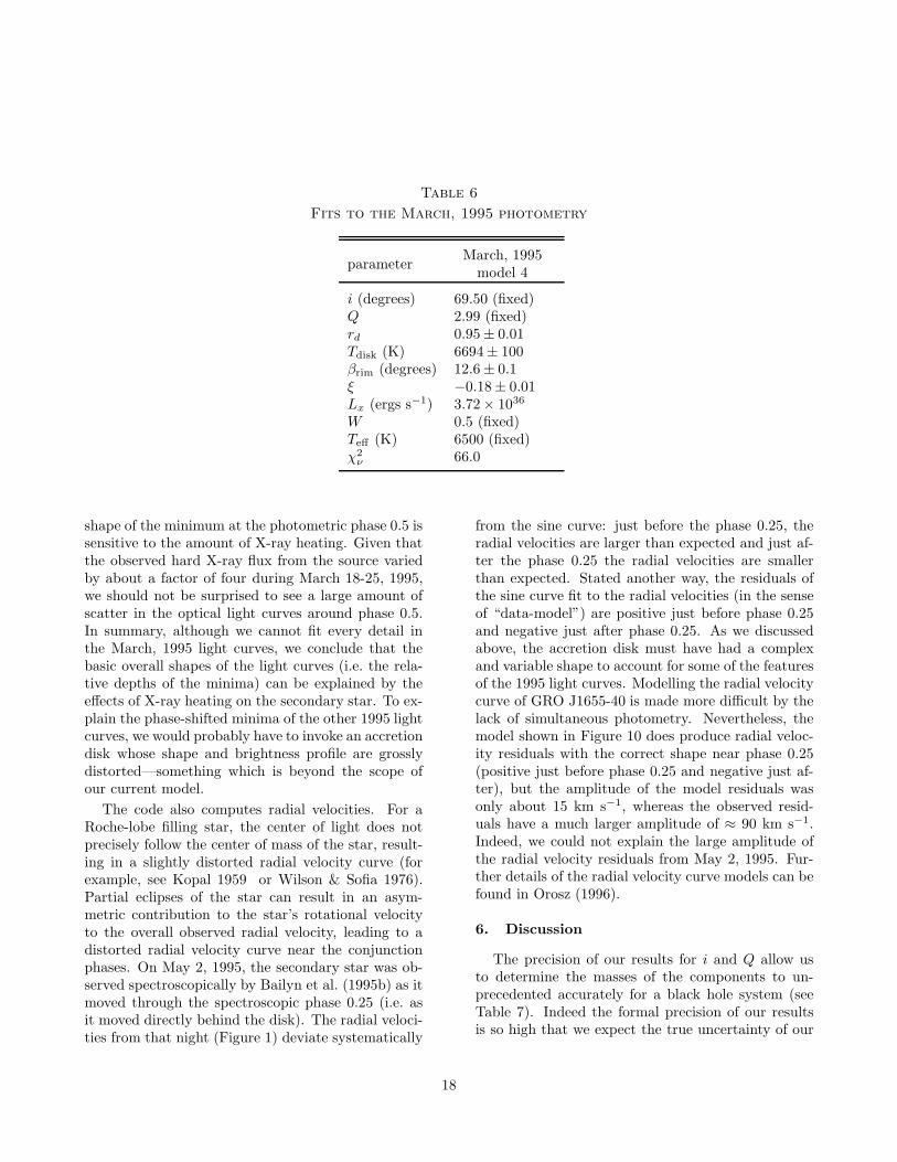
Table 6

Fits to the March, 1995 photometry

parameterMarch, 1995model 4

i (degrees) 69.50 (fixed)Q 2.99 (fixed)rd 0.95± 0.01Tdisk (K) 6694± 100βrim (degrees) 12.6± 0.1ξ −0.18± 0.01Lx (ergs s−1) 3.72× 1036

W 0.5 (fixed)Teff (K) 6500 (fixed)χ2ν 66.0

shape of the minimum at the photometric phase 0.5 issensitive to the amount of X-ray heating. Given thatthe observed hard X-ray flux from the source variedby about a factor of four during March 18-25, 1995,we should not be surprised to see a large amount ofscatter in the optical light curves around phase 0.5.In summary, although we cannot fit every detail inthe March, 1995 light curves, we conclude that thebasic overall shapes of the light curves (i.e. the rela-tive depths of the minima) can be explained by theeffects of X-ray heating on the secondary star. To ex-plain the phase-shifted minima of the other 1995 lightcurves, we would probably have to invoke an accretiondisk whose shape and brightness profile are grosslydistorted—something which is beyond the scope ofour current model.

The code also computes radial velocities. For aRoche-lobe filling star, the center of light does notprecisely follow the center of mass of the star, result-ing in a slightly distorted radial velocity curve (forexample, see Kopal 1959 or Wilson & Sofia 1976).Partial eclipses of the star can result in an asym-metric contribution to the star’s rotational velocityto the overall observed radial velocity, leading to adistorted radial velocity curve near the conjunctionphases. On May 2, 1995, the secondary star was ob-served spectroscopically by Bailyn et al. (1995b) as itmoved through the spectroscopic phase 0.25 (i.e. asit moved directly behind the disk). The radial veloci-ties from that night (Figure 1) deviate systematically

from the sine curve: just before the phase 0.25, theradial velocities are larger than expected and just af-ter the phase 0.25 the radial velocities are smallerthan expected. Stated another way, the residuals ofthe sine curve fit to the radial velocities (in the senseof “data-model”) are positive just before phase 0.25and negative just after phase 0.25. As we discussedabove, the accretion disk must have had a complexand variable shape to account for some of the featuresof the 1995 light curves. Modelling the radial velocitycurve of GRO J1655-40 is made more difficult by thelack of simultaneous photometry. Nevertheless, themodel shown in Figure 10 does produce radial veloc-ity residuals with the correct shape near phase 0.25(positive just before phase 0.25 and negative just af-ter), but the amplitude of the model residuals wasonly about 15 km s−1, whereas the observed resid-uals have a much larger amplitude of ≈ 90 km s−1.Indeed, we could not explain the large amplitude ofthe radial velocity residuals from May 2, 1995. Fur-ther details of the radial velocity curve models can befound in Orosz (1996).

6. Discussion

The precision of our results for i and Q allow usto determine the masses of the components to un-precedented accurately for a black hole system (seeTable 7). Indeed the formal precision of our resultsis so high that we expect the true uncertainty of our

18

Table 7

Component masses for GRO J1655-40

confidencelimit

i(degrees)

QM1

(M⊙)M2

(M⊙)

1σ 69.42-69.58 2.91-3.07 6.80-7.24 2.20-2.463σ 69.00-70.60 2.60-3.45 6.42-7.63 1.86-2.90

results comes from physical effects not included inthe models. However, given the good fit between ourmodels and the data, we expect that the systematicerrors are also quite small. In the following we discussthe implications of our results for the nature of thesecondary star, the radio jet, the evolutionary historyof the system, and the outburst mechanism. We willuse the parameters listed in Table 7 for the systemthroughout the following discussion.

6.1. Luminosity and Nature of the Secondary

Star

The mass ratio of Q = 2.99 ± 0.08 we found forGRO J1655-40 is the smallest among the seven blackhole systems with low mass secondaries. Much largervalues of Q have been found for the three systemswhere the mass ratio has been directly computed viathe measurement of the rotational broadening of thesecondary star’s absorption lines: Q = 14.9 for bothA0620-00 (Marsh, Robinson, & Wood 1994) and V404Cyg (Casares 1995), and Q = 23.8 for GS 2000+25(Harlaftis, Horne, & Filippenko 1996). There arehints that the mass ratio may be extreme in XNMus91 (Orosz et al. 1994), and GRO J0422+32 (Fil-ippenko, Matheson, & Ho 1995) as well. In GROJ1655-40, we have a way to independently check thevalue of the mass ratio by comparing the observedluminosity of the secondary star to the luminosity in-ferred from the model fits. To compute the observedluminosity in V , we adopt a mean V magnitude ofV = 17.12, which is the mean of the model fit to theMarch, 1996 data, a distance of d = 3.2 ± 0.2 kpc(which is tightly constrained by the kinematics of theradio jets—see Hjellming & Rupen 1995), a disk frac-tion in V of 5%±2% (Section 4), and a color excess ofE(B−V ) = 1.3±0.1 (Horne et al. 1996; Horne privatecommunication 1996). Assuming a visual extinctionof Av = 3.1E(B−V ), the observed luminosity in V of

the GRO J1655-40 secondary is Lobs = 46.6±13.6L⊙.

The luminosity of the secondary star inferred fromthe models is easily derived from some simple rela-tions. Given the measured masses and orbital periodof the system, we can use Kepler’s Third Law to deter-mine the semi-major axis. Eggleton’s (1983) expres-sion for the effective radius of the Roche lobe thendetermines the size of the secondary, and the temper-ature inferred from the spectral type and the Stefan-Boltzmann Law determines the luminosity. Figure 11shows the computed mass, radius, and luminosity ofthe secondary star as a function of Q, assuming an in-clination of i = 69.5 deg, an effective temperature ofTeff = 6500 K, and an orbital period of 2.d62157. Thevertical dashed line in the three panels indicates thevalue of Q from the best model fit, and the horizontaldashed and dotted lines in the lower panel indicate theobserved luminosity of the GRO J1655-40 secondaryand its 1σ error. Evidently, models with Q ∼< 3.5 areneeded to produce a secondary star with a luminositylarge enough to match the observed luminosity of theGRO J1655-40 secondary. Models with larger massratios (i.e. Q

∼> 5) not only produce under-luminous

secondary stars, but also provide fits to the data withrelatively large χ2

ν values (Figure 7). The agreementbetween the luminosity of the secondary calculatedfrom the orbital parameters and that inferred fromthe known distance and reddening of the source pro-vides a satisfying consistency check for our models.

The observed luminosity of the GRO J1655-40 sec-ondary star is a fairly well-constrained quantity, ow-ing to the fact that the distance is well determinedfrom the kinematics of the radio jets (Hjellming &Rupen 1995) and the amount of interstellar extinc-tion is well determined from high quality UV spec-tra obtained with the Hubble Space Telescope (Horneet al. 1996). The observed spectral type of the starprovides a fairly good measure of its effective tem-

19

Fig. 11.— The mass (top), radius (middle), and the luminosity (bottom) of the secondary star as a function of themass ratio Q, assuming Teff = 6500 K, i = 69.5 deg, f(M) = 3.24M⊙, and P = 2.d62157. The dashed and dottedlines in the lower panel indicate the observed luminosity of the secondary star in GRO J1655-40 and its 1σ error.

perature (e.g. Straizys & Kuriliene 1981), and weadopt Teff = 6500 ± 250 K. We therefore can accu-rately place the secondary star of GRO J1655-40 on aHertzsprung-Russell diagram (Figure 12). Using theYale Stellar Evolution Code (Guenther et al. 1992)with updated opacities (Iglesias & Rogers 1996), wecomputed the evolutionary tracks of a 2.1M⊙ star,a 2.3M⊙ star, and a 2.5M⊙ star, assuming a so-lar metallicity, a hydrogen abundance of 71%, and amixing length coefficient of 1.7, all typical values forpopulation I stars. These evolutionary tracks are alsoshown in Figure 12. The secondary star falls very nearthe track of the 2.3M⊙ star, roughly halfway betweenthe main sequence and the giant branch. This pro-vides yet another consistency check for our model. Itis interesting to note the radius of the 2.3M⊙ starnear the position of the secondary: 690 Myr after thezero-age main sequence (ZAMS) the star has a ra-dius of 4.85R⊙ (and a temperature of Teff = 6813 Kand a luminosity of L2 = 45.8L⊙); 692 Myr afterthe ZAMS, the star has a radius of 5.21R⊙ (andTeff = 6500 K and L2 = 43.8L⊙). ForQ = 2.99±0.08and i = 69.50±0.08 deg, the effective radius of the sec-ondary star is 4.85± 0.08R⊙ (when given the values

of the orbital period and mass function listed in Table2). Thus, the observed luminosity, the observed tem-perature, and the inferred radius of the GRO J1655-40 secondary star are all consistent with a ≈ 2.3M⊙single star that has evolved ≈ 690 × 106 years pastthe ZAMS.

6.2. Inclination of the Radio Jet

Hjellming & Rupen (1995) showed that the rel-ativistic radio jets GRO J1655-40 possessed duringlate 1994 were inclined 85± 2 deg to the line of sight.In addition, the jets were apparently rotating aboutthe jet axis at an angle of 2 deg and with a periodof 3.d0 ± 0.d2. Our light curve models show that theorbital plane is inclined 69.5 deg to the line of sight.Hence, the jet axis was tilted by 15.5 deg from thenormal of the orbital plane. If the jet axis was per-pendicular to the orbital plane, the 2 deg offset mightbe explained by a warped accretion disk near the com-pact object. In this case, the roughly three day peri-odicity would be closely related to the orbital periodof the binary since the orientation of the warp woulddepend on the orbital phase. However, since the jet

20

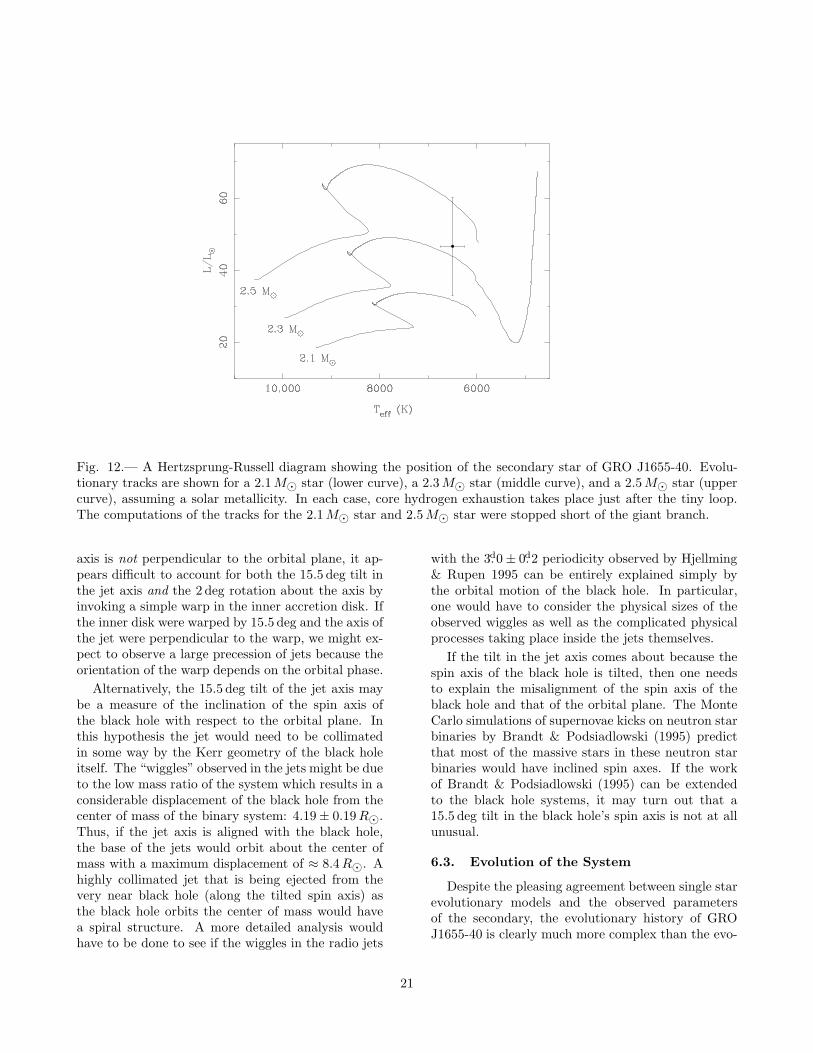
Fig. 12.— A Hertzsprung-Russell diagram showing the position of the secondary star of GRO J1655-40. Evolu-tionary tracks are shown for a 2.1M⊙ star (lower curve), a 2.3M⊙ star (middle curve), and a 2.5M⊙ star (uppercurve), assuming a solar metallicity. In each case, core hydrogen exhaustion takes place just after the tiny loop.The computations of the tracks for the 2.1M⊙ star and 2.5M⊙ star were stopped short of the giant branch.

axis is not perpendicular to the orbital plane, it ap-pears difficult to account for both the 15.5 deg tilt inthe jet axis and the 2 deg rotation about the axis byinvoking a simple warp in the inner accretion disk. Ifthe inner disk were warped by 15.5 deg and the axis ofthe jet were perpendicular to the warp, we might ex-pect to observe a large precession of jets because theorientation of the warp depends on the orbital phase.

Alternatively, the 15.5 deg tilt of the jet axis maybe a measure of the inclination of the spin axis ofthe black hole with respect to the orbital plane. Inthis hypothesis the jet would need to be collimatedin some way by the Kerr geometry of the black holeitself. The “wiggles” observed in the jets might be dueto the low mass ratio of the system which results in aconsiderable displacement of the black hole from thecenter of mass of the binary system: 4.19± 0.19R⊙.Thus, if the jet axis is aligned with the black hole,the base of the jets would orbit about the center ofmass with a maximum displacement of ≈ 8.4R⊙. Ahighly collimated jet that is being ejected from thevery near black hole (along the tilted spin axis) asthe black hole orbits the center of mass would havea spiral structure. A more detailed analysis wouldhave to be done to see if the wiggles in the radio jets

with the 3.d0± 0.d2 periodicity observed by Hjellming& Rupen 1995 can be entirely explained simply bythe orbital motion of the black hole. In particular,one would have to consider the physical sizes of theobserved wiggles as well as the complicated physicalprocesses taking place inside the jets themselves.

If the tilt in the jet axis comes about because thespin axis of the black hole is tilted, then one needsto explain the misalignment of the spin axis of theblack hole and that of the orbital plane. The MonteCarlo simulations of supernovae kicks on neutron starbinaries by Brandt & Podsiadlowski (1995) predictthat most of the massive stars in these neutron starbinaries would have inclined spin axes. If the workof Brandt & Podsiadlowski (1995) can be extendedto the black hole systems, it may turn out that a15.5 deg tilt in the black hole’s spin axis is not at allunusual.

6.3. Evolution of the System

Despite the pleasing agreement between single starevolutionary models and the observed parametersof the secondary, the evolutionary history of GROJ1655-40 is clearly much more complex than the evo-

21

lutionary history of a single star (e.g. Webbink 1992;van den Heuvel 1992; Webbink & Kalogera 1994).Webbink & Kalogera (1994) give several conditionsfor the successful formation of a low mass X-ray bi-nary, some of the conditions being: (i) the progenitorbinary must have an extreme mass ratio in order todrive the system to a common envelope and the initialbinary must be wide enough to survive the commonenvelope stage; (ii) the post-common-envelope binarymust be big enough to accommodate the secondarystar within its Roche lobe and wide enough to allowthe primary to evolve to core collapse; and (iii) thebinary system must survive the core collapse. If theconditions stated by Webbink & Kalogera (1994) aremet and we are left with a 7M⊙ black hole with a2.3M⊙ main sequence companion star in an orbitwith a period of about 2.6 days, the subsequent bi-nary evolution will dominated by the evolution of thesecondary star since the timescale for the evolution ofthat 2.3M⊙ star is much shorter than the timescalefor the loss of orbital angular momentum (King, Kolb,& Burderi 1996). The orbit is not likely to be left cir-cular after the core collapse, but tidal dissipation willcircularize the orbit before the secondary can fill itsRoche lobe (Webbink & Kalogera 1994). Once theorbit is circularized, the stellar evolution computa-tions we performed show that on a timescale of order690 million years, the companion star will evolve offthe main sequence and attain a radius, luminosity,and temperature comparable to the secondary star ofGRO J1655-40 that we see today. The radius the starattains is roughly the effective radius of the Rochelobe of the secondary star in GRO J1655-40.

GRO J1655-40 stands out among the black holebinaries in that it has a large space velocity (i.e. ithas a large γ velocity, see Table 3 and Brandt, Pod-siadlowski, & Sigurdsson [1995, hereafter BPS95]).BPS95 argued that GRO J1655-40 may have ac-quired its velocity as the result of a kick caused byan asymmetry during the initial collapse of the com-pact object (as is thought to be the case with neu-tron stars—Brandt & Podsiadlowski 1995; Johnston1996). BPS95 proposed that the black hole in GROJ1655-40 formed via an intermediate neutron stage,and was then converted into a black hole by additionalaccretion from the secondary star or through somekind of phase transition in the cooling compact object.This scenario predicts that the final black hole binarysystem should have a large mass ratio and that themasses of the components would be relatively small

(M1 ≈ 3.6M⊙ and M2 ≈ 0.3M⊙). However, our fitsto the light curves show that almost the opposite sit-uation is true: the mass ratio Q is relatively close tounity and the masses of the components are relativelylarge (M1 = 7M⊙ and M2 = 2.3M⊙). Therefore, ifthe compact object passed through an intermediateneutron stage, it would have had to accrete ∼> 5M⊙to attain its present day mass, with the accreted mat-ter presumably coming from the companion star. Aswe showed above, the position of the secondary staron the Hertzsprung-Russell diagram is consistent withthe track of a normal 2.3M⊙ star halfway betweenthe main sequence and the giant branch. If the sec-ondary star was once much more massive and it gaveup most of its mass to the compact primary, its evo-lutionary path on the Hertzsprung-Russell diagramcould be quite different than that of a normal 2.3M⊙star. Thus, BPS95’s proposed scenario of the for-mation of the black hole in GRO J1655-40 seems tobe less viable in view of the large amount of matterthe compact object must accrete and the secondarystar must give up in order to attain their present-daymasses. If the compact object initially formed as aneutron star, it seems likely that a significant amountof material from the supernova itself must have fallenback, thus converting the neutron star into a blackhole shortly after its creation. Note that the same su-pernova kick invoked by BPS95 to explain the largevelocity of GRO J1655-40 might also give rise to asubstantial tilt in the spin axis of the compact objectas discussed in Section 6.2.

6.4. Outburst Mechanism

Recently, King et al. (1996) and van Paradijs(1996) discussed the transient behavior in some lowmass X-ray binaries. In general, a system will be tran-sient if the average mass transfer rate M is smallerthan some critical value. In the case of GRO J1655-40 where the main sequence lifetime of the secondarystar is much shorter than the timescale of the shrink-age of the orbit due to angular momentum loss, theaverage mass loss rate is given by King et al. (1996)as

− M2 ≈ 4× 10−10P 0.93d M1.47

2 M⊙ yr−1 (2)

where Pd is the orbital period in units of days andwhere the units of M2 are solar masses. For GROJ1655-40, M2 = 3.4 × 10−9M⊙ yr−1 = 2.16 ×

1017 g s−1. This average mass transfer rate is muchlarger than the average mass transfer rates foundin the other six transient black hole systems, which

22

all have rates around 10−10M⊙ yr−1 (van Paradijs1996). For X-ray heated accretion disks, the criticalmass transfer rate is given by

Mcrit ≈ 5× 10−11M2/31 P

4/33 M⊙ yr−1 (3)

where the units of M1 are solar masses and whereP3 = P/(3 hr) (King et al. 1996). For GRO J1655-40,Mcrit = 1.1 × 10−8M⊙ yr−1. Thus GRO J1655-40is not expected to be a persistent X-ray source sinceM < Mcrit. It is, however, interesting to note howclose GRO J1655-40 is to being a persistent X-raysource. van Paradijs (1996) gives the following rela-tion dividing systems with stable and unstable masstransfer:

log Lx = 35.8 + 1.07 logP (hr) (4)

where Lx is the time-averaged X-ray luminosity overone outburst cycle. If a system falls below the line de-fined by Equation 4 in the P − Lx plane, then it willbe a transient system. If the energy generation rate is0.2c2 per gram of accreted matter (van Paradijs 1996),the averaged mass transfer rate of = 2.16×1017 g s−1

for GRO J1655-40 corresponds to an average X-ray lu-minosity of Lx = 3.88× 1038 erg s−1. This is slightlysmaller than the value of Lx = 5.31 × 1038 erg s−1

predicted from the relation given by Equation (4).The other six transient black hole systems have av-erage X-ray luminosities that are at least a factor often less than the critical X-ray luminosity defined byEquation 4 (see Figure 2 of van Paradijs 1996), whichsuggests that GRO J1655-40 is likely to have morefrequent X-ray outbursts than the other six transientblack hole systems. Indeed, there were several ad-ditional hard X-ray outbursts after the initial hardX-ray outburst observed July, 1994 (Harmon et al.1995a), and the soft X-ray outburst observed in lateApril, 1996 (Remillard et al. 1996a) came less thanone year after the sequence of hard X-ray outburstsended.

7. Summary

Using our database of GRO J1655-40 spectra, wehave established much improved values of the orbitalperiod (P = 2.d62157 ± 0.d00015), the radial velocitysemiamplitude (K2 = 228.2± 2.2 km s−1), the massfunction (f(M) = 3.24± 0.09M⊙), and MK spectraltype (F3IV to F6IV). Our photometry taken while thesystem was in true X-ray quiescence shows that lightfrom the distorted secondary star dominates, making

it possible to model the light curves in detail. Ourmodel of a distorted secondary star plus a circular ac-cretion disk provide excellent fits to the light curvestaken during true X-ray quiescence. We can add theeffects of X-ray heating on the secondary star and fitthe general shape of the March 18-25, 1995 V and Ilight curves, taken during a period of intense activityin hard X-rays. The best values of the orbital inclina-tion angle i and the mass ratio Q (i = 69.50±0.08 degand Q = 2.99±0.08) may be combined with the massfunction to give, for the first time, a reliable mass fora black hole: M1 = 7.02 ± 0.22M⊙. The positionof the secondary star on the Hertzsprung-Russell dia-gram is well determined, and its luminosity, tempera-ture, and radius are all consistent with a 2.3M⊙ star≈ 690 million years into its evolution past the ZAMS.The average mass accretion rate of the system is muchlarger than the averaged accretion rates of the othertransient black hole systems, putting GRO J1655-40much closer to the threshold where it would be a per-sistently strong X-ray source.

We are grateful to Sydney Barnes and Dana Di-nescu who assisted with the observations, and to thestaff of CTIO for the excellent support, in particularSrs. Maurico Navarrete, Edgardo Cosgrove, MauricoFernandez, & Luis Gonzalez. We thank the CTIOTime Allocation Committee for their flexible schedul-ing of the spectroscopy run on the 1.5 meter tele-scope. Alison Sills and Sukyong Yi kindly providedthe stellar evolution tracks for us. Mr. Yi also gaveus the digitized versions of the standard filter re-sponse curves. We thank Nan Zhang for providing uswith the BATSE daily flux averages from late March,1995. We acknowledge useful discussions with CraigRobinson, Jeffrey McClintock, Ronald Remillard, andRichard Wade. Financial support for this work wasprovided by the National Science Foundation througha National Young Investigator grant to C. Bailyn.

A. Appendix: The Eclipsing Light Curve

Code

In this Appendix we describe in detail the codeused to model the eclipsing light curve of GRO J1655-40. This program is a modified version of code firstwritten by Yoram Avni (Avni & Bahcall 1975; Avni1978; see also McClintock & Remillard 1990). Wewill outline here in detail the basic input physics andapproximations used, not to take credit for the work

23

of Avni and others, but to tell the readers exactlywhat the code does and how it does it.

A.1. The Potential

Consider a binary system consisting of a visiblestar of mass M2 and a compact object of mass M1,where the visible star orbits in a circular orbit witha Keplerian angular velocity ωk. Assume the visi-ble star is also rotating with an angular velocity ω2.Following the notation in Avni (1978), we define arectangular coordinate system with the origin at thecenter of the visible star, and with the X-axis point-ing towards the compact object, and the Z-axis inthe direction of ~ωk. This coordinate system rotateswith the visible star. The potential can be written as(Avni 1978)

Ψ(X,Y, Z) = −GM2

D

[

1

r2+

Q

r1−Qx

+Ω2(x2 + y2)(1 +Q)

2

]

(A1)

where D is the separation of the two stars, Q =M1/M2, Ω = ω2/ωk, r1 and r2 are the distance tothe centers of the two stars in units of D, and wherex and y, are X and Y in units of D. If Ω = 1 (thevisible star is in synchronous rotation), the poten-tial given by Equation (A1) reduces to the standardRoche potential, and the star can be in hydrostaticequilibrium in the rotating frame (Avni 1978). Thedegree to which the star fills its Roche lobe must bespecified—it is usually taken to be 100%.

In practice, it is convenient to adopt units of massand distance such that the GM1/D = 1. Typically,the star is assumed to be in synchronous rotation,so that Ω = 1, and it is assumed that it completelyfills its Roche lobe. Thus the value of the mass ratioQ uniquely determines the function for the potential,and hence the geometry of the Roche surface. Oncethe value of Q is specified, the visible star is dividedinto Nφ grid points in longitude φ, where the pointsare spaced equally in cosφ, and 4Nθ grid points inthe co-latitude θ, where the points are spaced equallyin the angle θ. The value of the potential Ψ and itsderivatives are then computed for each point.

A.2. Photometric Parameters

von Zeipel’s Theorem (1924) provides a relation-ship between the local gravity and the local emergentflux in a tidally distorted star. Proofs of von Zeipel’s

Theorem may be found in Kopal & Kitamura (1968)and Avni (1978). Using von Zeipel’s Theorem, onecan show that the light emitted from every point onthe photosphere of the star is the same as the lightemitted from a plane-parallel atmosphere character-ized by the local values of the temperature Te andgravity g:

T 4e ∝ g. (A2)

As a consequence of von Zeipel’s Theorem, the tem-perature at any point on the star is given by

T (x, y, z)

Tpole

=

[

g(x, y, z)

gpole

]β

, (A3)

where Tpole and gpole are the temperature and gravityat the pole of the star (i.e. the point on the surfaceof the star where the positive Z-axis emerges). The“gravity darkening exponent” β has two values: 0.25for stars with radiative atmospheres as shown by vonZeipel (1924), and 0.08 for stars with fully convectiveenvelopes (Lucy 1967). Thus, to specify the temper-ature T (x, y, z) at every point on the star, one mustinput the value of Tpole. This input temperature isusually taken to be the effective temperature of a fieldstar with a similar spectral type as the star to be mod-elled. In our model, the surface gravity on each pointon the star can be computed from the derivatives ofthe potential:

g(x, y, z) = −

[

(

∂Ψ

∂x

)2

+

(

∂Ψ

∂y

)2

+

(

∂Ψ

∂z

)2]1/2

(A4)e.g. (Zhang, Robinson, & Stover 1986).

Once the temperature is computed for each sur-face point, Planck’s function is used to approximatethe relationship between the temperature and themonochromatic intensity

I(λ) ∝

[

exp

(

hc

kλTe

)

− 1

]

−1

, (A5)

where h, c, and k are the usual physical constants.The star appears darker near its limb, a phenomenonreferred to as limb darkening. The code presently usesa standard linear limb darkening law expressed as

I(λ) ∝ 1− u(λ) + u(λ) cosµ, (A6)

where µ is the angle between the surface normal andthe line of sight. The values of the coefficient u(λ)are taken from standard tables computed from model

24

atmospheres (e.g. Al-Naimiy 1978). The reader is re-ferred to Kopal (1959), Kopal & Kitamura (1968),and Avni (1978) for more discussions on these ap-proximations.

A.3. Integration of the Flux from the Star

Let L(λ) be the radiation emitted by the star atthe wavelength λ as seen at a great distance. IfI(λ, x, y, z) is the intensity of the light at a surfacepoint, the total observed flux is given by

L(λ) =

∫

I(λ, x, y, z) cos γ ds, (A7)

where γ is the angle of foreshortening, ds is the sur-face element, and where the integration is to be doneover the entire visible surface of the star (Kopal &Kitamura 1968).

To carry out the numerical integration of the flux,some quantities need to be defined. First, each pointon the surface has direction cosines:

ℓx = cosφ

ℓy = sinφ cos θ

ℓz = sinφ sin θ. (A8)

The element of the surface area dS(x, y, z) is given by

dS(x, y, z) =R2∆φ∆θ

σ(x, y, z)(A9)

where R2 = x2 + y2 + z2, ∆φ and ∆θ are the gridsizes in longitude and co-latitude, respectively, andwhere

σ(x, y, z) = −ℓx

g(x, y, z)

(

∂Ψ(x, y, z)

∂x

)

−ℓy

g(x, y, z)

(

∂Ψ(x, y, z)

∂y

)

−ℓz

g(x, y, z)

(

∂Ψ(x, y, z)

∂z

)

.(A10)

Next, let Θ be the orbital phase of the observation(where Θ = 0 corresponds to the time of the clos-est approach of the visible star) and let i be the in-clination of the orbit (i = 90 deg for an orbit seenedge-on). The foreshortening Γ(x, y, z) of a partic-ular point on the star depends on the phase of theobservation, the inclination, and on the (x, y, z) coor-dinates of the point:

Γ(x, y, z) = −1

g(x, y, z)

(

sin i cosΘ∂Ψ(x, y, z)

∂x

)

+1

g(x, y, z)

(

sin i sinΘ∂Ψ(x, y, z)

∂y

)

+1

g(x, y, z)

(

cos i∂Ψ(x, y, z)

∂z

)

.(A11)

If the “projection factor” Γ(x, y, z) < 0, then thatparticular point is not visible. At each phase, theflux elements from the visible points (i.e. those withΓ(x, y, z) > 0) are simply summed up:

Lstar(Θ, λ) =

Nφ∑

i=1

4Nθ∑

j=1

I(λ, x, y, z)Γ(x, y, z)dS(x, y, z),

(A12)where each pair of (i, j) indices are associated witha specific (x, y, z) point on the star. In practice, theabove sum in Equation (A12) converges effectively forNφ ≥ 40 and Nθ ≥ 14.

So far, Equations (A1) through (A12) describe thebasic input physics and mathematics of the originalAvni code (Avni & Bahcall 1975; Avni 1978). Thiscode models the light curve due to a single Rochelobe filling star. Extra sources of light such as lightdue to X-ray heating effects are not taken into ac-count in the Avni code. To summarize the model sofar, the user specifies the degree to which the starfills its Roche lobe (usually 100%), the value of themass ratio Q, and the rate of the star’s rotation (usu-ally Ω = 1 for synchronous rotation). These threequantities define the shape of the surface of the star.Then the user must specify the polar temperature ofthe star Tpole, the gravity darkening exponent β (ei-ther 0.25 or 0.08 depending on whether the star hasa radiative envelope or a convective envelope), andthe linearized limb darkening coefficient u(λ) appro-priate for the star in question in order to compute thetemperatures over the surface of the star. Once thetemperatures are known, the Planck function and alinearized limb darkening law are used to compute theintensities over the surface. Finally, after the orbitalphase and the inclination of the orbit are specified,the total observed flux can be computed.

A.4. The Addition of an Accretion Disk

To make the basic Avni code more realistic, weadded an accretion disk to the code. Following Zhanget al. (1986), the disk is flattened cylinder centered onthe (invisible) compact object. The plane of the or-bit bisects the disk in the z-direction. The disk is as-sumed to be completely optically thick, so that we canonly see light from its surface and so that anything

25

behind the disk is completely eclipsed. The face of thedisk is divided up into several grids equally spaced inthe polar coordinates (r, α). The outer radius of thedisk rd is scaled to a user specified fraction of theeffective Roche lobe radius of the primary and the in-ner radius ri is set to a very small number (typically0.005). Eggleton’s (1983) approximation is used tocompute the effective Roche lobe radius. The thick-ness of the disk at the outer edge is zd = 2rd tanβrim.With the exception of user-defined “hot-spots”, thetemperature of the disk does not vary with the az-imuth angle. The radial distribution of the tempera-ture across the face of the disk is given by

T (r) = Tdisk(r/rd)ξ, (A13)

where Tdisk is the user specified temperature at theouter edge of the disk. For a steady-state, opticallythick, viscous accretion disk, the power law exponentξ = −0.75 (Pringle 1981). As before, Planck’s func-tion is used to approximate the relationship betweenthe temperature of a point on the surface of the diskand the monochromatic intensity Idisk(λ, r, α) of thatpoint.

Recently Diaz, Wade, & Hubeny (1996) discussedthe importance of including corrections for limb dark-ening in models of disk spectra. Limb darkening is im-portant for disks since the limb darkening correctionsdepend on the temperature (and hence the radius inour model) and on the effective wavelength. There-fore the slope of a blackbody disk’s spectrum will bein error if no limb darkening corrections are made.An important result of the work of Diaz et al. (1996)is that the limb darkening law in the optically thickrings of their accretion disk models is very similar tothe limb darkening law in a stellar atmosphere. As aresult, one may use the same linearized limb darken-ing coefficients for disks that one uses for stars. Wetherefore have

Idisk(λ, r, α) ∝ 1− udisk(λ, T (r))

+udisk(λ, T (r)) cos i (A14)

where the values of udisk(λ, T (r)) are interpolatedfrom tables given by Wade & Rucinski (1985).

The foreshortening angle of the normal of a surfaceelement on the face of the disk is simply cos i. In theabsence of eclipses, the observed flux from the face of

the accretion disk is:

Ldisk(Θ, λ) =

Nr∑

i=1

Nα∑

j=1

Idisk(λ, r, α)(cos i) r∆r∆α,

(A15)where Nr and Nα are the number of grid points in ra-dius and azimuth, respectively, where ∆r and ∆α arethe grid spacings in radius and azimuth, and whereeach pair of (i, j) indices are associated with a specific(r, α) point on the disk.

To handle the situations where the disk has a sub-stantial thickness, light from the rim is also accountedfor. The rim is divided into 11 grid points in the zdirection, and Nα grid points in azimuth. The tem-perature of the rim is Tdisk, and the intensities of eachrim point are found using Planck’s function. If the az-imuth angle α is measured from the X-axis, then theforeshortening factor Γrim(α) of a point on the rim atthe orbital phase Θ is

Γrim(α) = sin i cos(α+Θ). (A16)

If Γrim(α) < 0, the point is hidden. A limb darkeningcorrection is made for the edge surface elements basedon the value of Γrim(α):

Irim(λ, α) ∝ 1− udisk(λ, Tdisk)

+udisk(λ, Tdisk)Γrim(α) (A17)

The total flux from the rim is found by summing theintensities of all visible points:

Lrim(Θ, λ) =

11∑

i=1

Nα∑

j=1

Irim(λ, α)Γrim(α)∆z∆α,

(A18)where ∆z is the step size in the Z direction, andwhere each pair of (i, j) indices are associated with aspecific (z, α) point on the rim.

Hot spots can be added to the disk. The spots areconfined to radii rcut ≤ r ≤ rd and azimuth anglesαi1 ≤ α ≤ αi

2, where at the moment i = 0 (no spots),1 or 2. The temperature of the spot Tspot is added tothe temperature T (r, α) of each point on the disk rimand face that lies inside the spot boundaries. The in-tensities of each point are computed as before and theintegrations are carried out as before (e.g. Equations(A15) and (A18)).

In the absence of eclipses, the total observed fluxfrom the star and the disk is

Ltotal(Θ, λ) = Lstar(Θ, λ) + Ldisk(Θ, λ) + Lrim(Θ, λ).(A19)

26

A.5. The Addition of Eclipses

In the case where the inclination angle i is largeenough to allow for eclipses, the procedure for com-puting the light curves must be modified slightly.First, the intensities of each point on the star, diskface, and disk rim are computed from the list of in-put parameters. We can determine which body is infront of the other body from the orbital phase Θ—the star will obviously be closer than the disk for0 deg ≤ Θ ≤ 90 deg or for 270 deg ≤ Θ ≤ 360 degand the other way around for 90 deg ≤ Θ ≤ 270 deg.The integration of the flux elements over the visiblesurface of the object in front is carried out as before.Then, all points on the edge of the body in front (i.e.its horizon) are determined and are projected onto theplane of the sky. The horizon of the eclipsing bodydefines some polygon on the plane of the sky. Then,as the integration of the flux elements of the body inback is carried out, each potentially visible point isprojected onto the plane of the sky and checked tosee if it falls inside the horizon of the eclipsing body.If the point is eclipsed, it is not included in the inte-gration. Once all of the visible points are included inthe integrations, the total observed flux is found asbefore (Equation (A19)).

A.6. The Addition of X-ray Heating

If the secondary star intercepts a large amount offlux from the other body (either X-ray heating fromthe vicinity of the compact object or optical lightfrom the disk), there may be a large amount of re-processed radiation. The irradiating flux can stronglyalter the distribution of temperatures across the faceof the star. A rigorous treatment of these “reflectioneffects” requires difficult and time-consuming compu-tations (e.g. Kopal 1959; Wilson & Devinney 1971).Following Zhang et al. (1986), we will use a simpli-fied treatment of the heating effects. We will consideronly heating of the star by X-ray heating, and not theheating of the disk by the star. For simplicity, all ofthe irradiating flux Firr due to the X-ray heating isassumed to come from the center of the compact ob-ject.

The total energy in X-rays intercepted by theRoche lobe filling secondary star does not depend onthe scale of the orbit since the surface area of Rochelobe filling star facing the X-ray source is proportionalto the square of the orbital separation. However, thechange in the star’s atmosphere caused by the X-ray

heating does depends on the size of the orbit. As thedistance between the star and the X-ray source is in-creased, each square centimeter on the star’s surfacereceives less energy in X-rays. The change in the lo-cal temperature depends on the amount of absorbedX-ray flux per unit area. So to find the magnitudeof the irradiating flux seen by each point on the sec-ondary, the X-ray luminosity of the X-ray source Lx

(in ergs s−1) and the physical size of the orbit mustbe specified. The code uses the mass function f(M)and the orbital period P to find the scale of the orbit.

The distance d (in units of the orbital separation)between each point on the face of the star and theX-ray source can be found

d(x, y, z) = (1 + z2 +R2− 2Rℓx), (A20)

where ℓx is one of the direction cosines (Equation(A8)), and where R2 = x2 + y2 + z2. The foreshort-ening factor ΓX−ray(x, y, z) is given by

ΓX−ray(x, y, z) =x(1 − x)− y2 + z2

Rd, (A21)

where ΓX−ray(x, y, z) < 0 indicates that the point onthe star cannot see the X-ray source. The amount ofX-ray flux each surface element intercepts is

Firr(x, y, z) =

(

Lx

4πa2d(x, y, z)2

)

ΓX−ray(x, y, z).

(A22)The modified temperature of each surface point thatcan see the X-ray source is given by

T 4X−ray(x, y, z) = T 4

pole

(

g(x, y, z)

gpole(x, y, z)

)4β

+WFirr

σ(A23)

whereW is the albedo, and σ is the Stefan-Boltzmannconstant (Zhang et al. 1986). The albedo W is notvery well determined, and it is usually set to 0.5 (seeZhang et al. 1986).

In the cases there the disk has a substantial thick-ness, some points on the face of the star may be be-low the rim of the disk as seen from the compact ob-ject. These points would not receive any X-ray fluxfrom the compact object and hence their tempera-tures would not change. It is easy to find the angleabove the plane that a point on the face of the starhas (as seen from the compact object):

Φ(x, y, z) = arctan

(

z

(1− x) cos η

)

(A24)

27

where η = arctan(y/x). This angle Φ(x, y, z) is com-pared to the angle of the rim βrim to see whetheror not the point on the star is blocked by the disk.If βrim > Φ(x, y, z), the point cannot see the X-raysource.

Once each point on the face of the star has beenassigned a new temperature based on the amount ofX-ray flux it sees, the intensities and the fluxes arefound following the procedures outlined above. Thenet result is that the points on the star facing the X-ray source are brighter than they would otherwise bebecause the temperatures were raised.

A.7. Filter Response Curves

We compute the total flux Ltotal(Θ, λ) at eachphase Θ for several values of the effective wavelengthλ using limb darkening coefficients u(λ) interpolatedfrom tables given by Wade & Rucinski (1985). Thismodel “spectrum” is integrated with the standardUBV RI filter response curves (Bessell 1990) to pro-duce model UBV RI magnitudes. In this way wecan perform simultaneous fits to light curves in sev-eral colors. In the case of GRO J1655-40, there is alarge amount of reddening in the light curves. Ratherthan attempting to include the reddening correctionin the fits, we instead fit the models to the normalizedBV RI data. In this way, the error of E(B − V ) doesnot enter into the analysis. We do, however, lose theabsolute color information contained in the model.

A.8. Light Curve Fitting and Error Analysis

We first compute a grid of models and χ2 fits to thedata using a wide range of parameters spaced in uni-form steps. Then several sets of parameters that pro-duce low χ2 values are chosen and are used as start-ing points for an optimization routine based on theGRIDLS program given in Bevington (1969). This“grid search” method was picked because it is easy toimplement and it does not require the computationof derivatives. After several runs with different start-ing points, the set of parameters that gives the lowestoverall χ2 fit to the data is chosen. By using severaldifferent starting points for the optimization routine,we can be reasonably sure that we have found theglobal minimum of χ2, rather than a local minimum.

We use three methods to estimate the statistical er-rors on the fitted parameters. The first one is a “boot-strap” method (Press et al. 1992). Artificial data setsare constructed from the original data set and the ex-

act fitting procedures which were used on the originaldata are used on the artificial data. The 1σ errorson the parameters are then derived from the distribu-tions of the fitted parameters from the many artificialdata sets. The second technique we use is outlined byZhang et al. (1986). Basically the 1σ error on a fit-ted parameter a0 is found by fixing the value of thatparameter at a new value a′0 = a0 + δ and findingthe values of the rest of the parameters a1 throughan that minimize χ2. The probable error of a0 is re-lated to the change in χ2 and to δ. We typically usetwo or three different values of δ (1%, 2%, and 3% ofthe value of the parameter) and average the resultingvalues of σ. Finally, the GRIDLS program given inBevington (1969) also provides error estimates basedon the shape of the chi-square hypersurface near theminimum. We used primarily the errors derived fromthe bootstrap method. We stress here that the er-rors estimated are only internal statistical errors, andnot systematic errors which we have no easy way tocompute.

REFERENCES

Al-Naimiy, H. M. 1978, Ap&SS, 53, 181

Avni, Y., & Bahcall, J. N. 1975, ApJ, 197, 675

Avni, Y. 1978, in “Physics and Astrophysics of Neu-tron Stars and Black Holes,” eds. R. Giacconi &R. Ruffini (Amsterdam: North-Holland), 42

Bailyn, C. D., et al. 1995a, Nature, 374, 701

Bailyn, C. D., Orosz, J. A., McClintock, J. E., &Remillard, R. A. 1995b, Nature, 378, 157

Bessell, M. S. 1990, PASP, 102, 1181

Bevington, P. R. 1969, “Data Reduction and ErrorAnalysis for the Physical Sciences,” (New York:McGraw-Hill Book Company)

Brandt, W. N., & Podsiadlowski, Ph. 1995, MNRAS,274, 461

Brandt, W. N., Podsiadlowski, Ph., & Sigurdsson, S.1995, MNRAS, 277, L35 (BPS95)

Campbell-Wilson, D., & Hunstead, R. 1994, IAU Cir-cular # 6052

Campbell-Wilson, D., & Hunstead, R. 1996, IAU Cir-cular # 6410

Casares, J. 1995, to be published in Proc. IAU Col-loquium 158 “Cataclysmic Variables and RelatedObjects”, 26-30 June 1995, Keele University, UK

28

Chevalier, C., & Ilovaisky, S. A. 1993, A&A, 269, 301

Diaz, M. P., Wade, R. A., & Hubeny, I. 1996, ApJ,459, 236

Eggleton, P. E. 1983, ApJ, 268, 368

Filippenko, A. V., Matheson, T., & Ho. L. C. 1995a,ApJ, 455, 614

Guenther, D. B., Demarque, P., Kim, Y.-C., & Pin-sonneault, M. H. 1992, ApJ, 387, 372

Harlaftis, E. T., Horne, K., & Filippenko, A. V.,PASP, in the press

Harmon, B. A., et al. 1995a, Nature, 374, 703

Harmon, B. A., et al. 1995b, IAU Circular #6205

Haswell, C. A., Robinson, E. L., Horne, K., Stiening,R. F., & Abbott, T. M. C. 1993, ApJ, 411, 802

Haswell, C. A. 1996, in “Compact Stars in Binaries,”IAU Symposium #165, eds J. van Paradijs, E. P.J. van den Heuvel, & E. Kuulkers, page 351

Hellier, C., & Mason, K. O. 1989, MNRAS, 239, 717

Hjellming, R. M., & Rupen, M. P. 1995, Nature, 375,464

Hjellming, R. M., & Rupen, M. P. 1996, IAU Circular#6411

Horne, K., et al. 1996, IAU Circular #6406

Iglesias, C. A., & Rogers, F. J. 1996, ApJ, 464, 943

Inoue, H., Nagase, F., Ishida, M., Sonobe, T., &Ueda, Y. 1994, IAU Circular #6063

Johnston, H. M. 1996, in “Evolutionary Processesin Binary Stars,” eds. R. A. M. J. Wijers, M. B.Davies, & C. A. Tout, (Kluwer Academic Publish-ers, Dordrecht), page 385

King, A. R., Kolb, U., & Burderi, L. 1996, ApJ, 464,L127

Kopal, Z. 1959, “Close Binary Systems”, The interna-tional Astrophysics Series Vol. 5 (New York: Chap-mann Hill & John Wiley)

Kopal, Z., & Kitamura, K. 1968, Advances in Astron-omy and Astrophysics, 6, 125.

Lucy, L. B. 1967, ZAp, 65, 89

Lucy, L. B., & Sweeney, M. A. 1971, AJ, 76, 544

Marsh, T. R., Robinson, E. L., & Wood, J. H. 1994,MNRAS, 266, 137

McClintock, J. E., & Remillard, R. A. 1986, ApJ, 308,110

McClintock, J. E., & Remillard, R. A. 1990, ApJ, 350,386

Morgan, W. W., & Keenan, P. C. 1973, ARA&A, 11,1973

Orosz, J. A., Bailyn, C. D., Remillard, R. A., Mc-Clintock, J. E., & Foltz, C. B. 1994, ApJ, 436, 848

Orosz, J. A., Bailyn, C. D., McClintock, J. E., &Remillard, R. A. 1996, ApJ, to appear September1, 1996

Orosz, J. A. 1996, Ph.D. Thesis, Yale University

Press, W. H., Teukolsky, S. A., Vetterling, W. T., &Flannery, B. P. 1992, “Numerical Recipes in For-tran: The Art of Scientific Computing,” secondedition, (Cambridge: Cambridge University Press)

Pringle, J. E. 1981, ARA&A, 19, 137

Remillard, R. A., et al. 1996a, IAU Circular #6393

Remillard, R. A., Orosz, J. A., McClintock, J. E., &Bailyn, C. D. 1996b, ApJ, 459, 226

Robinson, C., et al. 1996, ApJ, submitted

Stetson, P. B. 1987, PASP, 99, 191

Stetson, P. B., Davis, L. E., & Crabtree, D. R. 1991,in “CCDs in Astronomy,” ed. G. Jacoby, ASP Con-ference Series, Volume 8, page 282

Stetson, P. B. 1992a, in “Astronomical Data AnalysisSoftware and Systems I,” eds. D. M. Worrall, C.Biemesderfer, & J. Barnes, ASP Conference Series,Volume 25, page 297

Stetson, P. B. 1992b, in “Stellar Photometry—CurrentTechniques and Future Developments,” IAU Coll.136, eds. C. J. Butler, & I. Elliot, Cambridge Uni-versity Press, Cambridge, England, page 291

Straizys, V., & Kuriliene, G. 1981, Ap&SS, 80, 353

Tingay, S. J., et al. 1995, Nature, 374, 141

Tonry, J. & Davis, M. 1979, AJ, 84, 1511

van den Heuvel, E. P. J. 1992, in “X-ray Binaries andRecycled Pulsars,” eds. E. P. J. van den Heuvel& S. A. Rappaport, Kluwer Academic Publishers,Dordrecht, The Netherlands, page 233

van der Hooft, F., et al. 1996, MNRAS, submitted

van Paradijs, J. 1996, ApJ, 464, L139

von Zeipel, H. 1924, MNRAS, 84, 665

Wade, R. A., & Rucinski, S. M. 1985, A&AS, 60, 471

Wagner, R. M., Kreidl, T. J., Howell, S. B., & Star-rfield, S. G. 1992, ApJ, 401, L97

29

Webbink, R. F. 1992, in “X-ray Binaries and Recy-cled Pulsars,” eds. E. P. J. van den Heuvel & S.A. Rappaport, Kluwer Academic Publishers, Dor-drecht, The Netherlands, page 269

Webbink, R. F., & Kalogera, V. 1994, in “The Evolu-tion of X-ray Binaries”, AIP Conference Proceed-ings #308, eds. S. S. Holt & C. S. Day, page 321

Wilson, R. E., & Sofia, S. 1976, ApJ, 203, 182

Wilson, R. E., & Devinney, E. J. 1971, ApJ, 182, 539

Wilson, C. A., Harmon, B. A., Zhang, S. N., Paciesas,W. S., & Fishman, G. J. 1995, IAU Circular #6152

Zhang, E. -H., Robinson, E. L., & Stover, R. E. 1986,ApJ, 305, 740

Zhang, S. N., et al. 1994, IAU Circular #6046

This 2-column preprint was prepared with the AAS LATEXmacros v4.0.

30