Embed Size (px)
Citation preview
Optical Systems Design with Zemax OpticStudio
Lecture 1
Why Optical Systems Design
Optical system design is no longer a skill reserved for a few professionals. With readily available commercial optical design software, these tools are accessible to the general optical engineering community and rudimentary skills in optical design are now expected by a wide range of industries who utilize optics in their products.
Optical Systems Design 2
Course Aims
To introduce the design principles of lens and mirror optical systems and the evaluation of designs using modern computer techniques. The lectures will cover lens design, aberrations, optimization, tolerancing and image quality metrics.
Optical Systems Design 3
ZEMAX Optics Studio The ZEMAX optical design program is a comprehensive software tool. It integrates all the features required to conceptualize, design, optimize, analyze, tolerance, and document virtually any optical system. It is widely used in the optics industry as a standard design tool. This course will introduce the basics of ZEMAX using the recently released (2014) OpticStudio interface.
Optical Systems Design 4
Other Optical Design Software
• Code-V (Optical Research Associates) • OSLO (Sinclair Optics) • OpTaliX (Optenso Ltd) • ASAP (Breault Research) • TracePro (Lambda Research) • FRED (Photon Engineering)
Optical Systems Design 5
Course Outline
• Lecture 1: Introduction • Lecture 2: Sequential Systems • Lecture 3: Optimization • Lecture 4: Tolerancing • Lecture 5: Non-sequential & other stuff
Optical Systems Design 7
Web page: http://astro.dur.ac.uk/~rsharp/opticaldesign.html
Objectives: Lecture 1 At the end of this lecture you should: 1. Be able to install a version of the Zemax optical
design programme on a Windows PC 2. Understand the main tasks involved in optical
systems design with Zemax 3. Be aware of Zemax notation for the 5 main Seidel
aberrations 4. Know the relevance of the terms: optical axis,
stop, pupil, chief ray, marginal ray, point spread function for Zemax
5. Use the Zemax lens data editor to enter the specifications of a simple lens
Optical Systems Design 8
Recommended Texts • OpticStudio User Manual and Getting Started Using
OpticStudio (access from programme help) • Introduction to Lens Design with Practical Zemax
Examples, Joseph M Geary (Willmann-Bell Inc.) • Optical Systems Design, Robert Fischer & Bijana
Tadic(SPIE Press) • Practical Computer-Aided Design, Gregory Hallock-
Smith (Willmann-Bell Inc.) • Astronomical Optics, Dan Schroeder (Academic Press;
GoogleBooks) • Optics, Jeff Hecht (Addison Wesley)
Optical Systems Design 10
Also the Zemax knowledge base: http://www.zemax.com/support/knowledgebase
Optical Systems Design
‘Science or art of developing optical systems to image, direct, analyse or measure light.’ • Includes camera lenses, telescopes, microscopes, scanners, photometers, spectrographs, interferometers, … • Systems should be as free from geometrical optical errors (aberrations) as possible. • Correcting and controlling aberrations is one of the main tasks of the optical designer (includes performance evaluation and fabrication/tolerancing issues).
Optical Systems Design 11
Historical Note • Lens design has changed significantly since
~1960 with the introduction of digital computers and numerical optimisation.
• Equations describing aberrations of lens/mirror systems are very non-linear functions of system parameters (curvatures, spacings, refractive indices, dispersions, …)
• Only a few specialised systems can be derived analytically in exact closed-form solutions.
• Analytical design methods (Petzval, Seidel) were historically based on a mathematical treatment of geometrical imagery and primary aberrations – still useful for initial designs.
• Numerical evaluation methods ray trace many light rays from object to image space.
Optical Systems Design 12
Seidel (3rd order) Aberrations
1. Spherical aberration 2. Coma 3. Astigmatism 4. Field curvature 5. Distortion
Optical Systems Design 13
6. Longitudinal chromatic aberration 7. Lateral chromatic aberration
Numerical Evaluation Methods
• Assume only trigonometry, law of reflection and Snell’s law
• • For each ray calculate new ray parameters at each
surface • Sequential ray-tracing assumes that light travels
from surface to surface in a defined order. • Non-sequential ray-tracing does not assume a pre-
defined path for the rays, but when a ray hits a surface in its path, it may then reflect, refract, diffract, scatter or split into child rays (scattered light).
Optical Systems Design 14
n1 sinθ1 = n2 sinθ2
Numerical Optimisation Methods
• Given a starting configuration, the computer can be used to optimise a design by an iterative process.
• Final image quality is ‘best’ that can be achieved under constraints of basic configuration, required focal length, f/number, field of view, wavelength etc.
• Programs are still ‘dumb’. Designer must supply intelligence through selection of starting configuration, control of optimization parameters, understanding of underlying optical theory, etc.
Optical Systems Design 15
Objects, Light Rays & Wavefronts • Objects composed of self-luminous (radiant) points of
light • Trajectories of photons from each of these points
define the light rays • Neglecting diffraction, these physical rays become
geometrical rays (ray bundles) • Wavefronts are surfaces normal to rays • Light travel times along all rays to the wavefront from
an object point are the same (for a fixed wavelength) • Neglecting diffraction, physical wavefronts become
geometrical wavefronts (good approximation except near boundaries or edges)
Optical Systems Design 16
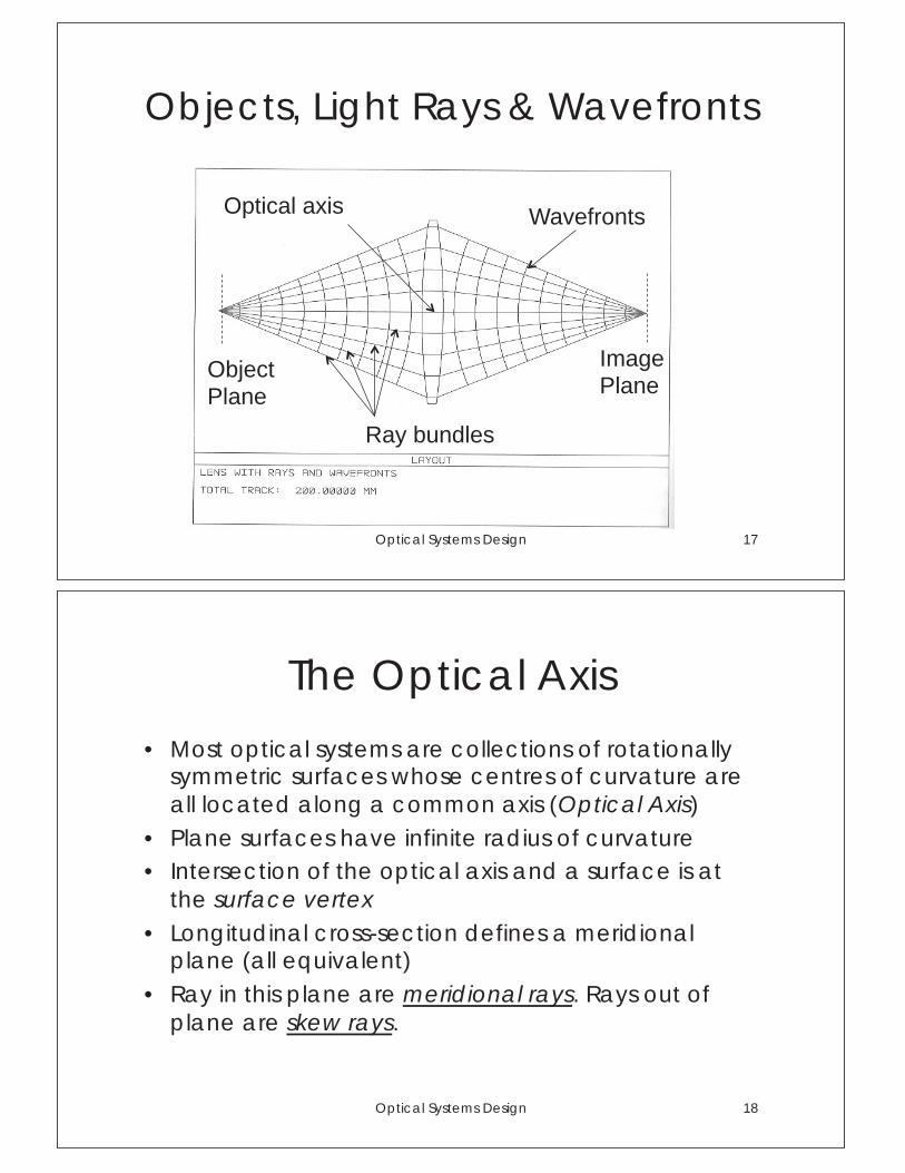
Objects, Light Rays & Wavefronts
Optical Systems Design 17
Object Plane
Image Plane
Optical axis Wavefronts
Ray bundles
The Optical Axis
• Most optical systems are collections of rotationally symmetric surfaces whose centres of curvature are all located along a common axis (Optical Axis)
• Plane surfaces have infinite radius of curvature • Intersection of the optical axis and a surface is at
the surface vertex • Longitudinal cross-section defines a meridional
plane (all equivalent) • Ray in this plane are meridional rays. Rays out of
plane are skew rays.
Optical Systems Design 18
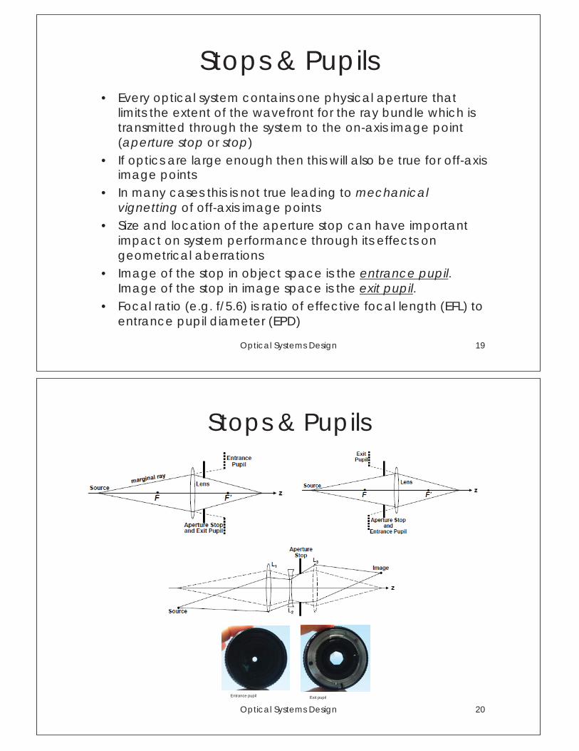
Stops & Pupils • Every optical system contains one physical aperture that
limits the extent of the wavefront for the ray bundle which is transmitted through the system to the on-axis image point (aperture stop or stop)
• If optics are large enough then this will also be true for off-axis image points
• In many cases this is not true leading to mechanical vignetting of off-axis image points
• Size and location of the aperture stop can have important impact on system performance through its effects on geometrical aberrations
• Image of the stop in object space is the entrance pupil. Image of the stop in image space is the exit pupil.
• Focal ratio (e.g. f/5.6) is ratio of effective focal length (EFL) to entrance pupil diameter (EPD)
Optical Systems Design 19
Stops & Pupils
Optical Systems Design 20
Entrance pupil Exit pupil
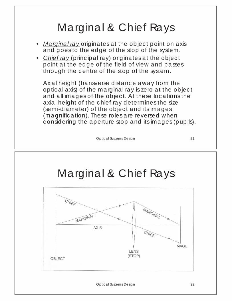
Marginal & Chief Rays • Marginal ray originates at the object point on axis
and goes to the edge of the stop of the system. • Chief ray (principal ray) originates at the object
point at the edge of the field of view and passes through the centre of the stop of the system.
Axial height (transverse distance away from the optical axis) of the marginal ray is zero at the object and all images of the object. At these locations the axial height of the chief ray determines the size (semi-diameter) of the object and its images (magnification). These roles are reversed when considering the aperture stop and its images (pupils).
Optical Systems Design 21
Marginal & Chief Rays
Optical Systems Design 22
Point Spread Function (PSF)
• Impossible to image a point object as a perfect point image.
• PSF gives the physically correct light distribution in the image plane including the effects of aberrations and diffraction.
• Errors are introduced by design (geometrical aberrations), optical and mechanical fabrication & alignment.
Optical Systems Design 23
Co-ordinate Systems and Sign Conventions
• No standardization between different codes!
• Zemax uses a right-handed cartesian co-ordinate system, where the Z-axis is the optical axis and light initially moves in the direction of +Z.
• Co-ordinate breaks (rotations) are defined in a right-handed sense.
Optical Systems Design 24
Optical Prescriptions
• An optical design is described by a set of surfaces through which the light passes sequentially.
• Surfaces are tabulated in the lens data editor and are numbered sequentially from the object surface (surface 0) and ending with the image surface.
• A minimum of 3 surfaces is required (object, stop, image).
Optical Systems Design 25
Surface Parameters
• Surface number • Radius of curvature (R) • Thickness to the next surface (t) • Glass type in the next medium (or Air if blank) • Aspheric data (if any) • Aperture size (semi-diameter D) • Tilt and decenter data (if any) One surface is designated the stop surface.
Optical Systems Design 26
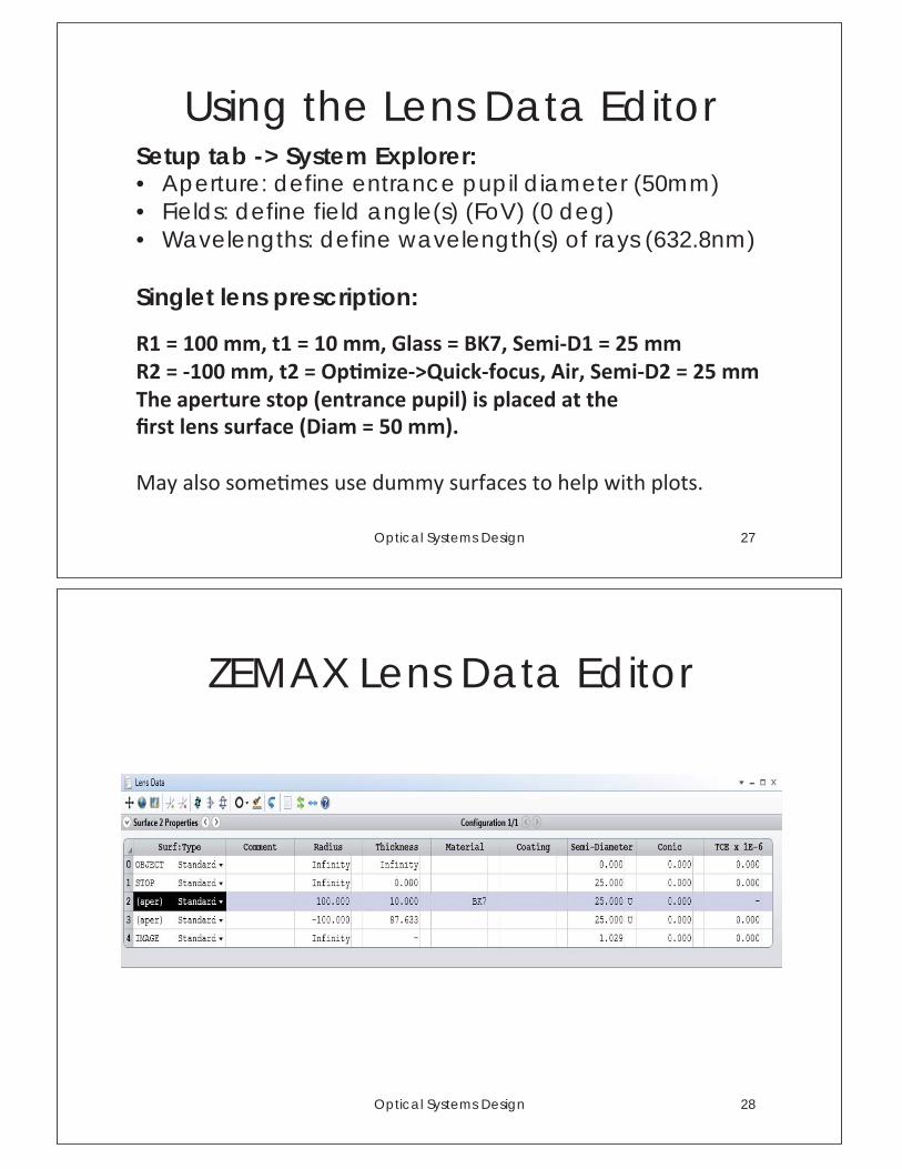
Using the Lens Data Editor Setup tab -> System Explorer: • Aperture: define entrance pupil diameter (50mm) • Fields: define field angle(s) (FoV) (0 deg) • Wavelengths: define wavelength(s) of rays (632.8nm) Singlet lens prescription:
Optical Systems Design 27
ZEMAX Lens Data Editor
Optical Systems Design 28
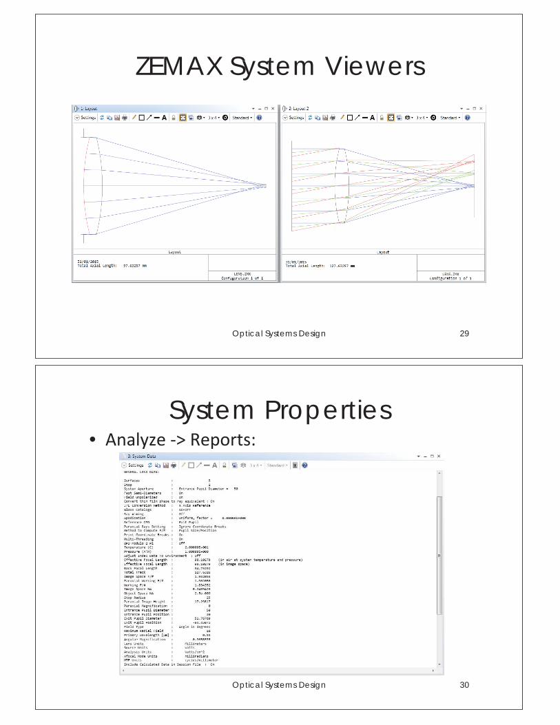
ZEMAX System Viewers
Optical Systems Design 29
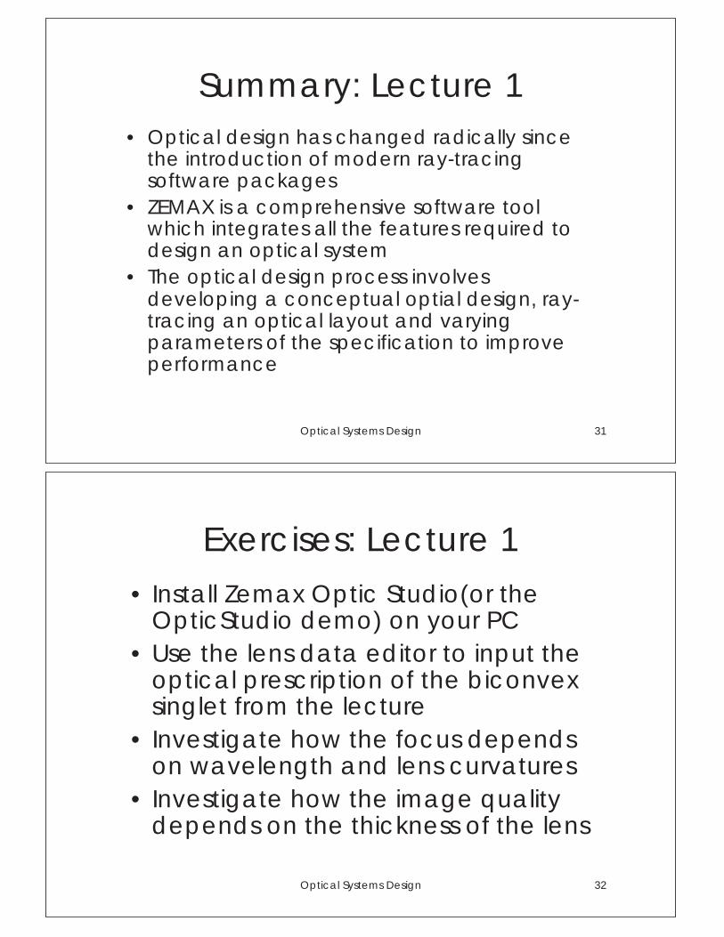
System Properties
Optical Systems Design 30
•
Summary: Lecture 1 • Optical design has changed radically since
the introduction of modern ray-tracing software packages
• ZEMAX is a comprehensive software tool which integrates all the features required to design an optical system
• The optical design process involves developing a conceptual optial design, ray-tracing an optical layout and varying parameters of the specification to improve performance
Optical Systems Design 31
Exercises: Lecture 1
• Install Zemax Optic Studio(or the OpticStudio demo) on your PC
• Use the lens data editor to input the optical prescription of the biconvex singlet from the lecture
• Investigate how the focus depends on wavelength and lens curvatures
• Investigate how the image quality depends on the thickness of the lens
Optical Systems Design 32
Sequential Ray Tracing
Lecture 2
Sequential Ray Tracing • Rays are traced through a pre-defined sequence of
surfaces while travelling from the object surface to the image surface.
• Rays hit each surface once in the order (sequence) in which the surfaces are defined. Particularly well-suited to imaging systems (including spectrometers).
• Numerically fast and extremely useful for the design, optimization and tolerancing of such systems.
• Aberrations evaluated using spot diagrams, ray fan plots, OPD plots, geometrical image analysis and MTF (physical optics) calculations.
February 15, 2016 Optical Systems Design 2
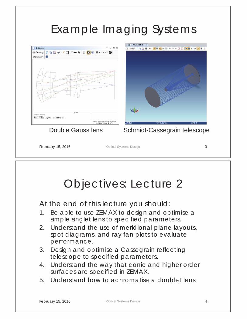
Example Imaging Systems
February 15, 2016 Optical Systems Design 3
Double Gauss lens Schmidt-Cassegrain telescope
Objectives: Lecture 2
At the end of this lecture you should: 1. Be able to use ZEMAX to design and optimise a
simple singlet lens to specified parameters. 2. Understand the use of meridional plane layouts,
spot diagrams, and ray fan plots to evaluate performance.
3. Design and optimise a Cassegrain reflecting telescope to specified parameters.
4. Understand the way that conic and higher order surfaces are specified in ZEMAX.
5. Understand how to achromatise a doublet lens.
February 15, 2016 Optical Systems Design 4
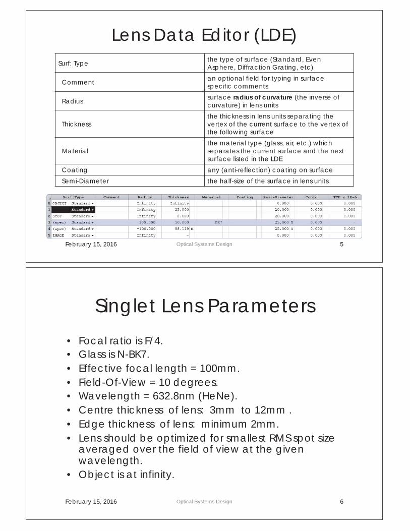
Lens Data Editor (LDE) Surf: Type
the type of surface (Standard, Even Asphere, Diffraction Grating, etc)
Comment an optional field for typing in surface specific comments
Radius surface radius of curvature (the inverse of curvature) in lens units
Thickness the thickness in lens units separating the vertex of the current surface to the vertex of the following surface
Material the material type (glass, air, etc.) which separates the current surface and the next surface listed in the LDE
Coating any (anti-reflection) coating on surface
Semi-Diameter the half-size of the surface in lens units
February 15, 2016 Optical Systems Design 5
Singlet Lens Parameters
• Focal ratio is F/4. • Glass is N-BK7. • Effective focal length = 100mm. • Field-Of-View = 10 degrees. • Wavelength = 632.8nm (HeNe). • Centre thickness of lens: 3mm to 12mm . • Edge thickness of lens: minimum 2mm. • Lens should be optimized for smallest RMS spot size
averaged over the field of view at the given wavelength.
• Object is at infinity.
February 15, 2016 Optical Systems Design 6
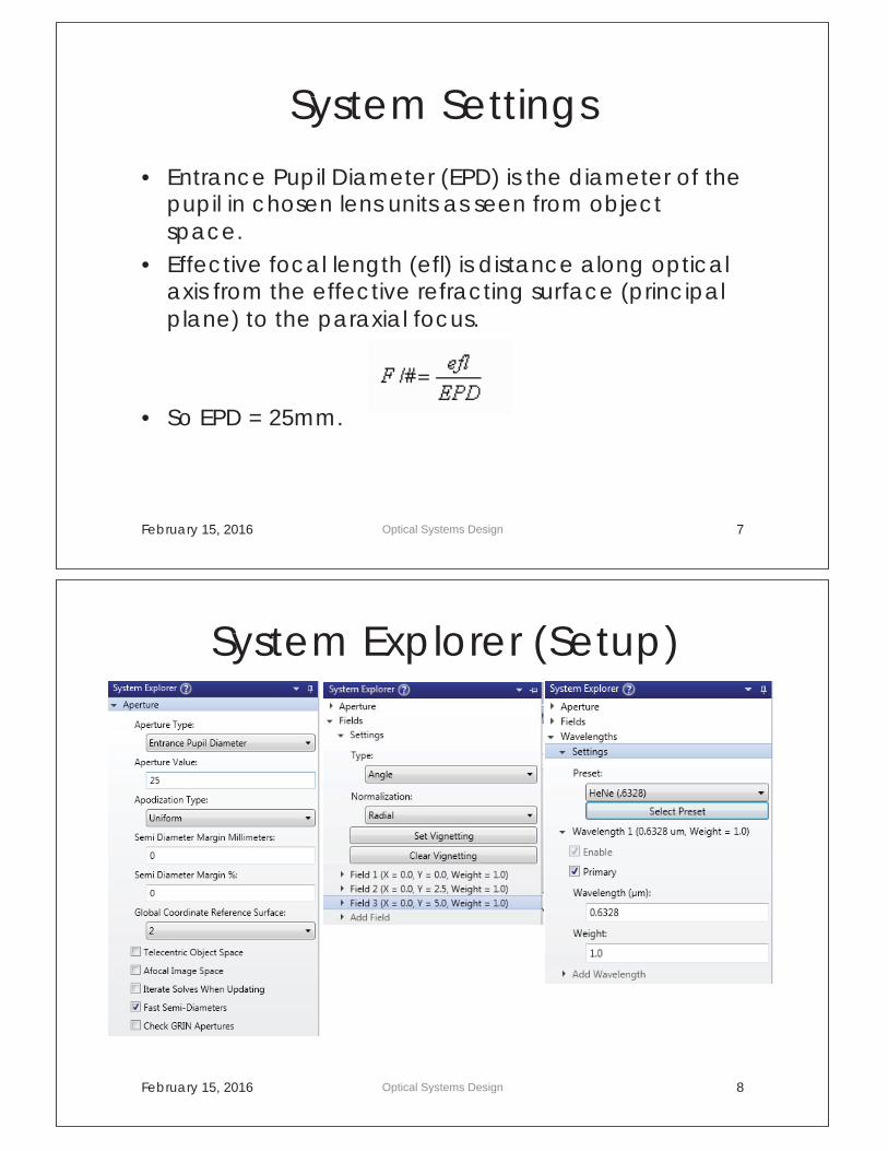
System Settings
• Entrance Pupil Diameter (EPD) is the diameter of the pupil in chosen lens units as seen from object space.
• Effective focal length (efl) is distance along optical axis from the effective refracting surface (principal plane) to the paraxial focus.
• So EPD = 25mm.
February 15, 2016 Optical Systems Design 7
System Explorer (Setup)
February 15, 2016 Optical Systems Design 8
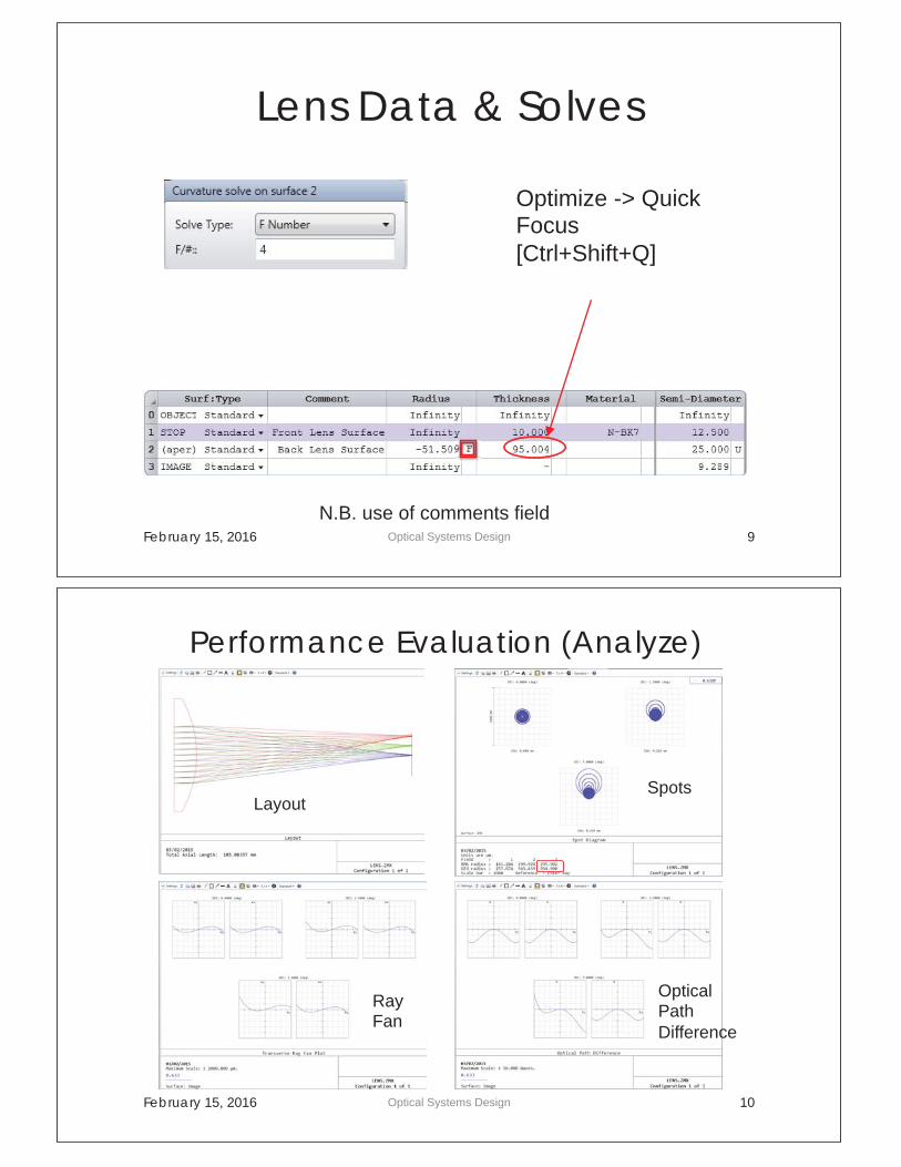
Lens Data & Solves
February 15, 2016 Optical Systems Design 9
N.B. use of comments field
Optimize -> Quick Focus [Ctrl+Shift+Q]
Performance Evaluation (Analyze)
February 15, 2016 Optical Systems Design 10
Layout
Optical Path Difference
Spots
Ray Fan
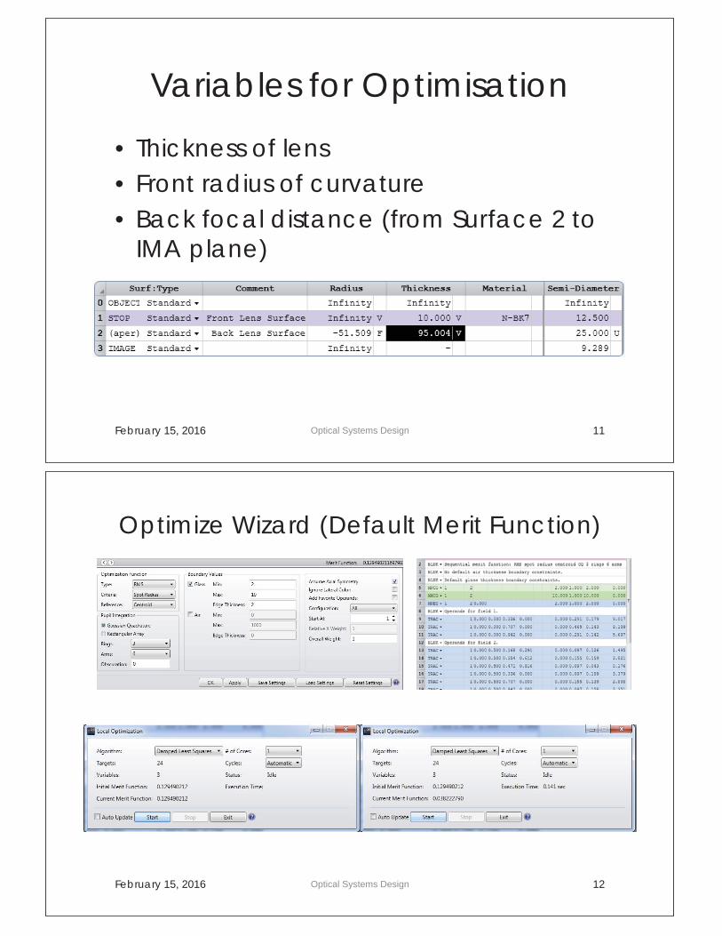
Variables for Optimisation
• Thickness of lens • Front radius of curvature • Back focal distance (from Surface 2 to
IMA plane)
February 15, 2016 Optical Systems Design 11
Optimize Wizard (Default Merit Function)
February 15, 2016 Optical Systems Design 12
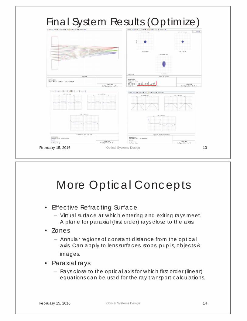
Final System Results (Optimize)
February 15, 2016 Optical Systems Design 13
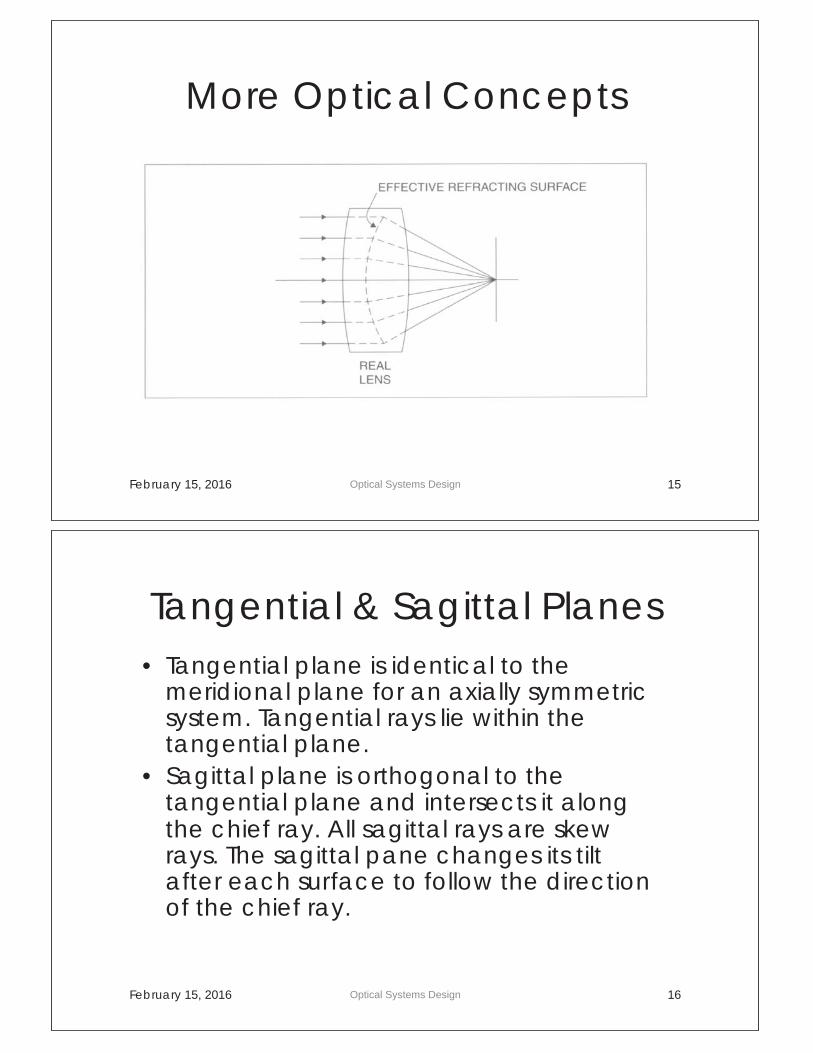
More Optical Concepts
• Effective Refracting Surface – Virtual surface at which entering and exiting rays meet.
A plane for paraxial (first order) rays close to the axis.
• Zones – Annular regions of constant distance from the optical
axis. Can apply to lens surfaces, stops, pupils, objects &
images. • Paraxial rays
– Rays close to the optical axis for which first order (linear) equations can be used for the ray transport calculations.
February 15, 2016 Optical Systems Design 14
More Optical Concepts
February 15, 2016 Optical Systems Design 15
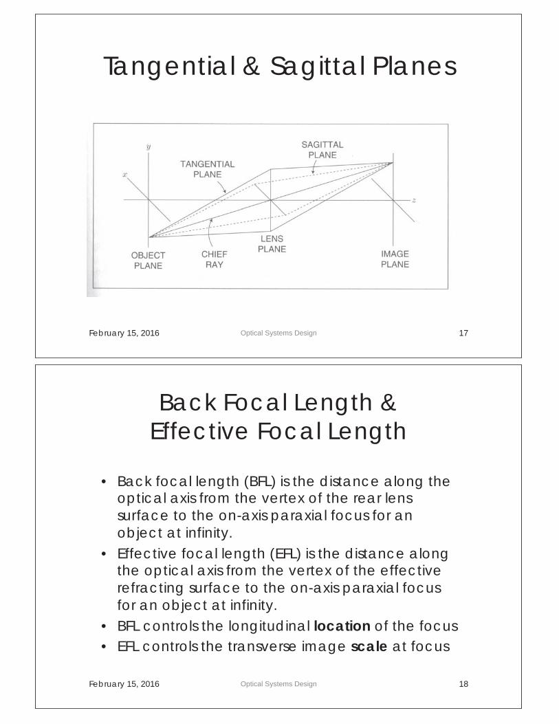
Tangential & Sagittal Planes • Tangential plane is identical to the
meridional plane for an axially symmetric system. Tangential rays lie within the tangential plane.
• Sagittal plane is orthogonal to the tangential plane and intersects it along the chief ray. All sagittal rays are skew rays. The sagittal pane changes its tilt after each surface to follow the direction of the chief ray.
February 15, 2016 Optical Systems Design 16
Tangential & Sagittal Planes
February 15, 2016 Optical Systems Design 17
Back Focal Length & Effective Focal Length
• Back focal length (BFL) is the distance along the optical axis from the vertex of the rear lens surface to the on-axis paraxial focus for an object at infinity.
• Effective focal length (EFL) is the distance along the optical axis from the vertex of the effective refracting surface to the on-axis paraxial focus for an object at infinity.
• BFL controls the longitudinal location of the focus • EFL controls the transverse image scale at focus
February 15, 2016 Optical Systems Design 18
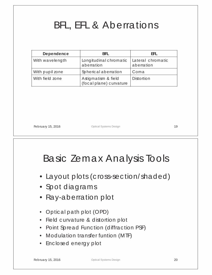
BFL, EFL & Aberrations
Dependence BFL EFL
With wavelength Longitudinal chromatic aberration
Lateral chromatic aberration
With pupil zone Spherical aberration Coma
With field zone Astigmatism & field (focal plane) curvature
Distortion
February 15, 2016 Optical Systems Design 19
Basic Zemax Analysis Tools
• Layout plots (cross-section/shaded) • Spot diagrams • Ray-aberration plot
• Optical path plot (OPD) • Field curvature & distortion plot • Point Spread Function (diffraction PSF) • Modulation transfer funtion (MTF) • Enclosed energy plot
February 15, 2016 Optical Systems Design 20
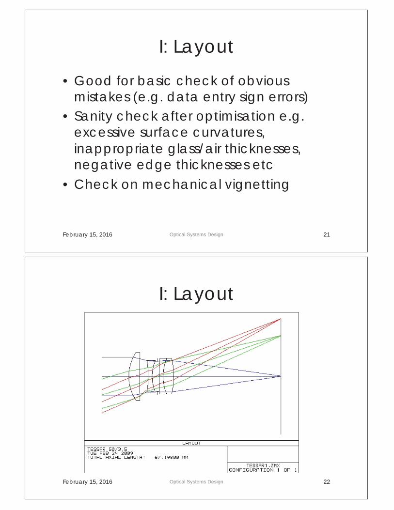
I: Layout
• Good for basic check of obvious mistakes (e.g. data entry sign errors)
• Sanity check after optimisation e.g. excessive surface curvatures, inappropriate glass/air thicknesses, negative edge thicknesses etc
• Check on mechanical vignetting
February 15, 2016 Optical Systems Design 21
I: Layout
February 15, 2016 Optical Systems Design 22
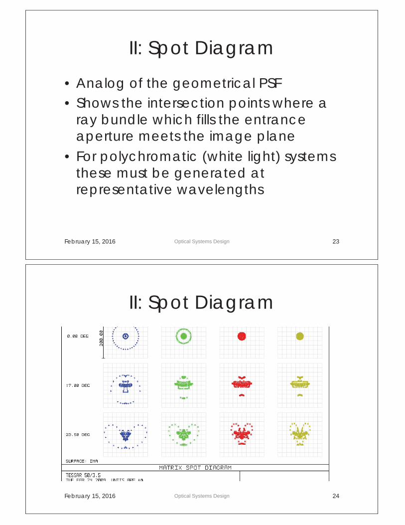
II: Spot Diagram
• Analog of the geometrical PSF • Shows the intersection points where a
ray bundle which fills the entrance aperture meets the image plane
• For polychromatic (white light) systems these must be generated at representative wavelengths
February 15, 2016 Optical Systems Design 23
II: Spot Diagram
February 15, 2016 Optical Systems Design 24
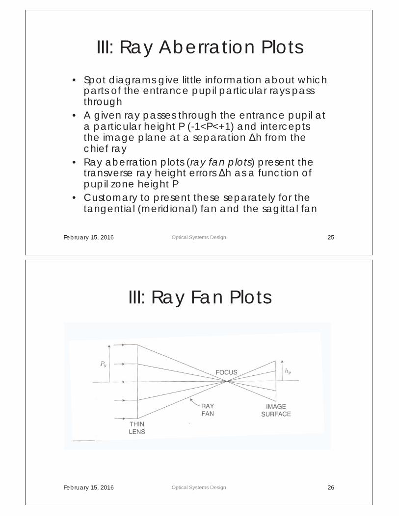
III: Ray Aberration Plots
• Spot diagrams give little information about which parts of the entrance pupil particular rays pass through
• A given ray passes through the entrance pupil at a particular height P (-1<P<+1) and intercepts the image plane at a separation Δh from the chief ray
• Ray aberration plots (ray fan plots) present the transverse ray height errors Δh as a function of pupil zone height P
• Customary to present these separately for the tangential (meridional) fan and the sagittal fan
February 15, 2016 Optical Systems Design 25
III: Ray Fan Plots
February 15, 2016 Optical Systems Design 26
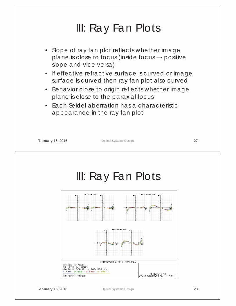
III: Ray Fan Plots
• Slope of ray fan plot reflects whether image plane is close to focus (inside focus → positive slope and vice versa)
• If effective refractive surface is curved or image surface is curved then ray fan plot also curved
• Behavior close to origin reflects whether image plane is close to the paraxial focus
• Each Seidel aberration has a characteristic appearance in the ray fan plot
February 15, 2016 Optical Systems Design 27
III: Ray Fan Plots
February 15, 2016 Optical Systems Design 28
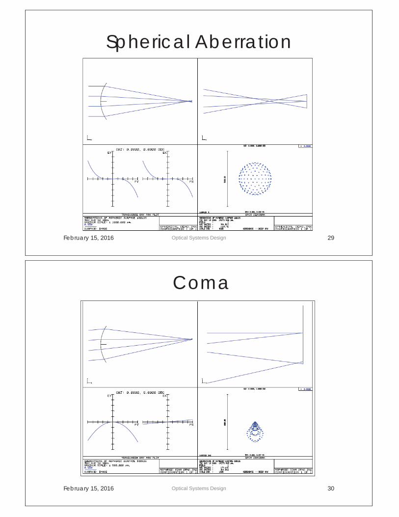
Spherical Aberration
February 15, 2016 Optical Systems Design 29
Coma
February 15, 2016 Optical Systems Design 30
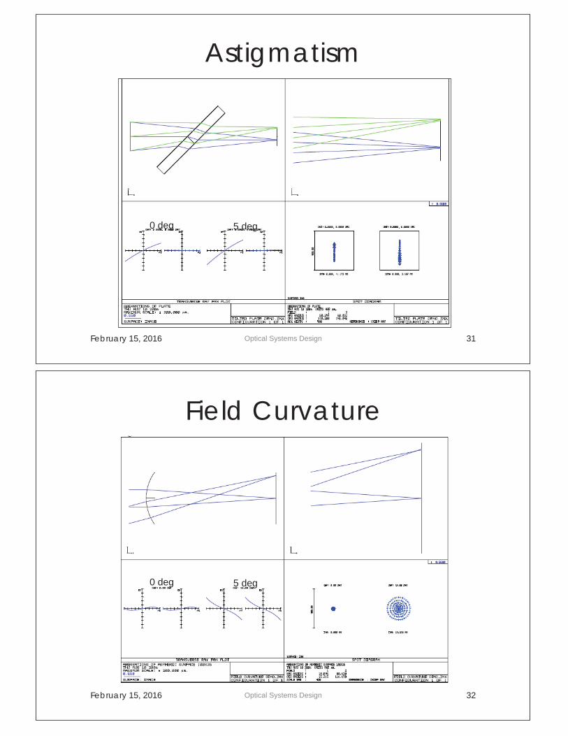
Astigmatism
February 15, 2016 Optical Systems Design 31
0 deg 5 deg
Field Curvature
February 15, 2016 Optical Systems Design 32
0 deg 5 deg
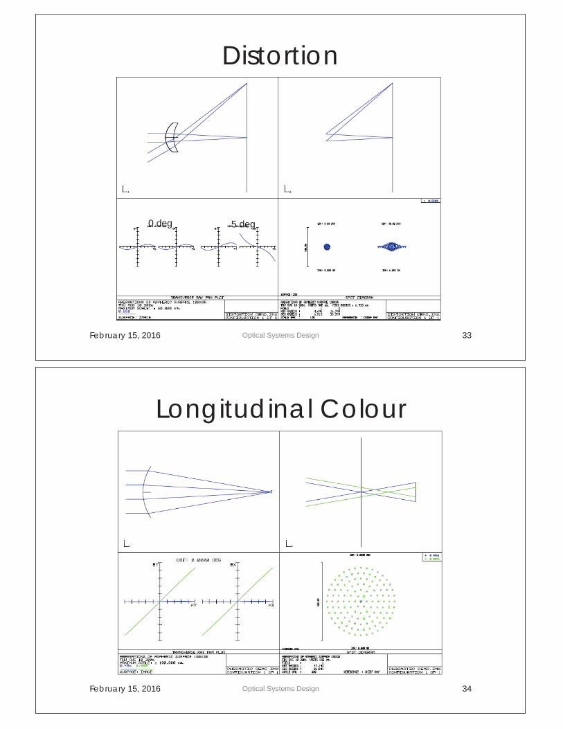
Distortion
February 15, 2016 Optical Systems Design 33
0 deg 5 deg
Longitudinal Colour
February 15, 2016 Optical Systems Design 34
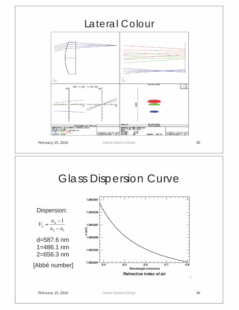
Lateral Colour
February 15, 2016 Optical Systems Design 35
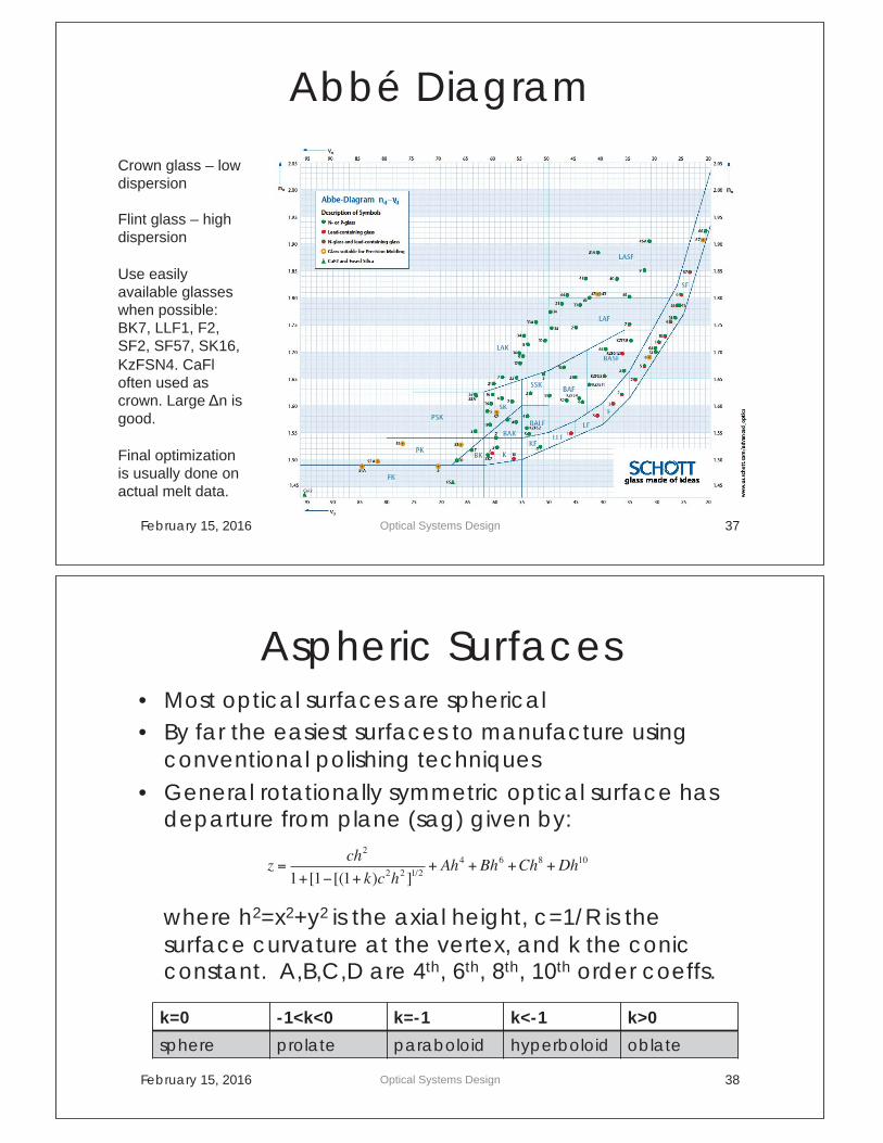
Glass Dispersion Curve
February 15, 2016 Optical Systems Design 36
Dispersion: d=587.6 nm 1=486.1 nm 2=656.3 nm
Vd =nd −1n2 − n1
[Abbé number]
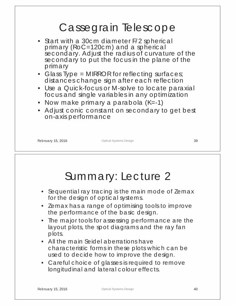
Abbé Diagram
February 15, 2016 Optical Systems Design 37
Crown glass – low dispersion Flint glass – high dispersion Use easily available glasses when possible: BK7, LLF1, F2, SF2, SF57, SK16, KzFSN4. CaFl often used as crown. Large Δn is good. Final optimization is usually done on actual melt data.
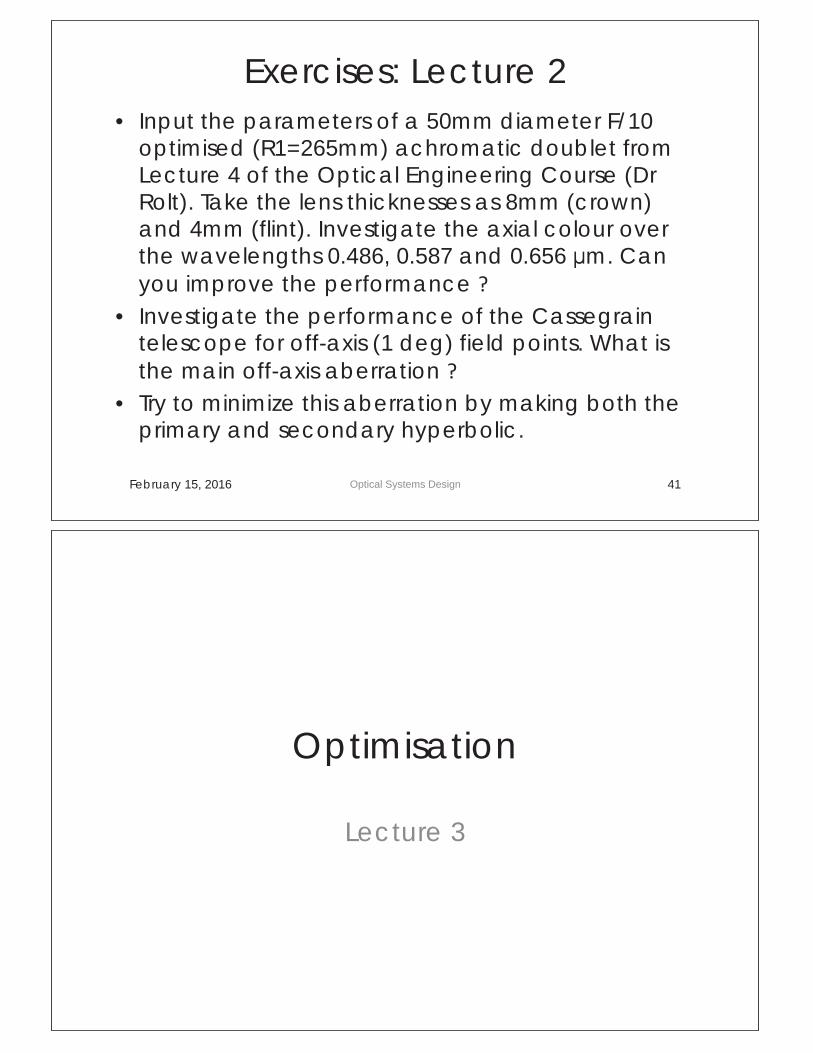
Aspheric Surfaces • Most optical surfaces are spherical • By far the easiest surfaces to manufacture using
conventional polishing techniques • General rotationally symmetric optical surface has
departure from plane (sag) given by: where h2=x2+y2 is the axial height, c=1/R is the
surface curvature at the vertex, and k the conic constant. A,B,C,D are 4th, 6th, 8th, 10th order coeffs.
February 15, 2016 Optical Systems Design 38
z =ch2
1+[1−[(1+ k)c2h2 ]1/2+ Ah4 +Bh6 +Ch8 +Dh10
k=0 -1<k<0 k=-1 k<-1 k>0
sphere prolate paraboloid hyperboloid oblate
Cassegrain Telescope • Start with a 30cm diameter F/2 spherical
primary (RoC=120cm) and a spherical secondary. Adjust the radius of curvature of the secondary to put the focus in the plane of the primary
• Glass Type = MIRROR for reflecting surfaces; distances change sign after each reflection
• Use a Quick-focus or M-solve to locate paraxial focus and single variables in any optimization
• Now make primary a parabola (K=-1) • Adjust conic constant on secondary to get best
on-axis performance
February 15, 2016 Optical Systems Design 39
Summary: Lecture 2 • Sequential ray tracing is the main mode of Zemax
for the design of optical systems. • Zemax has a range of optimising tools to improve
the performance of the basic design. • The major tools for assessing performance are the
layout plots, the spot diagrams and the ray fan plots.
• All the main Seidel aberrations have characteristic forms in these plots which can be used to decide how to improve the design.
• Careful choice of glasses is required to remove longitudinal and lateral colour effects.
February 15, 2016 Optical Systems Design 40
Exercises: Lecture 2 • Input the parameters of a 50mm diameter F/10
optimised (R1=265mm) achromatic doublet from Lecture 4 of the Optical Engineering Course (Dr Rolt). Take the lens thicknesses as 8mm (crown) and 4mm (flint). Investigate the axial colour over the wavelengths 0.486, 0.587 and 0.656 µm. Can you improve the performance
• Investigate the performance of the Cassegrain telescope for off-axis (1 deg) field points. What is the main off-axis aberration
• Try to minimize this aberration by making both the primary and secondary hyperbolic.
February 15, 2016 Optical Systems Design 41
Optimisation
Lecture 3
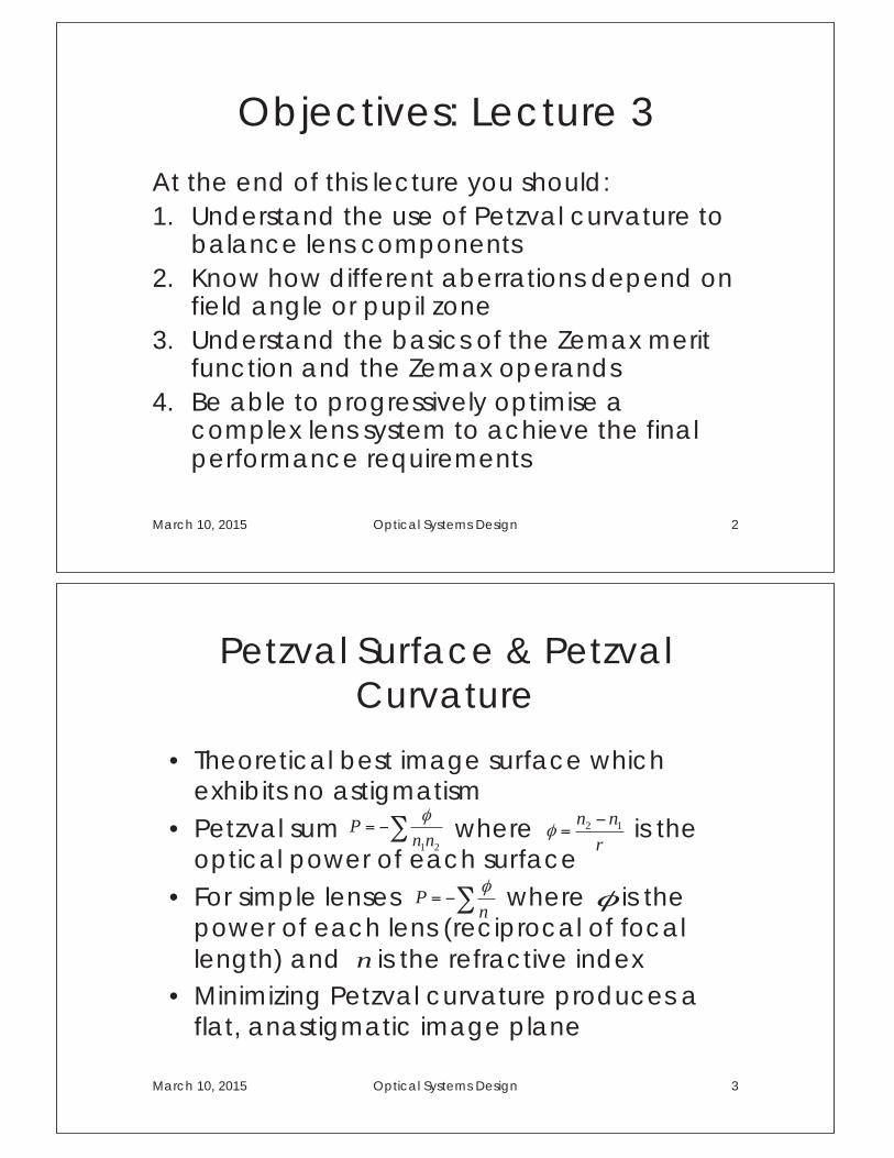
Objectives: Lecture 3
At the end of this lecture you should: 1. Understand the use of Petzval curvature to
balance lens components 2. Know how different aberrations depend on
field angle or pupil zone 3. Understand the basics of the Zemax merit
function and the Zemax operands 4. Be able to progressively optimise a
complex lens system to achieve the final performance requirements
March 10, 2015 Optical Systems Design 2
Petzval Surface & Petzval Curvature
• Theoretical best image surface which exhibits no astigmatism
• Petzval sum where is the optical power of each surface
• For simple lenses where is the power of each lens (reciprocal of focal length) and is the refractive index
• Minimizing Petzval curvature produces a flat, anastigmatic image plane
March 10, 2015 Optical Systems Design 3
∑−=21nn
P φ
rnn 12 −=φ
∑−= nP φ φ
n
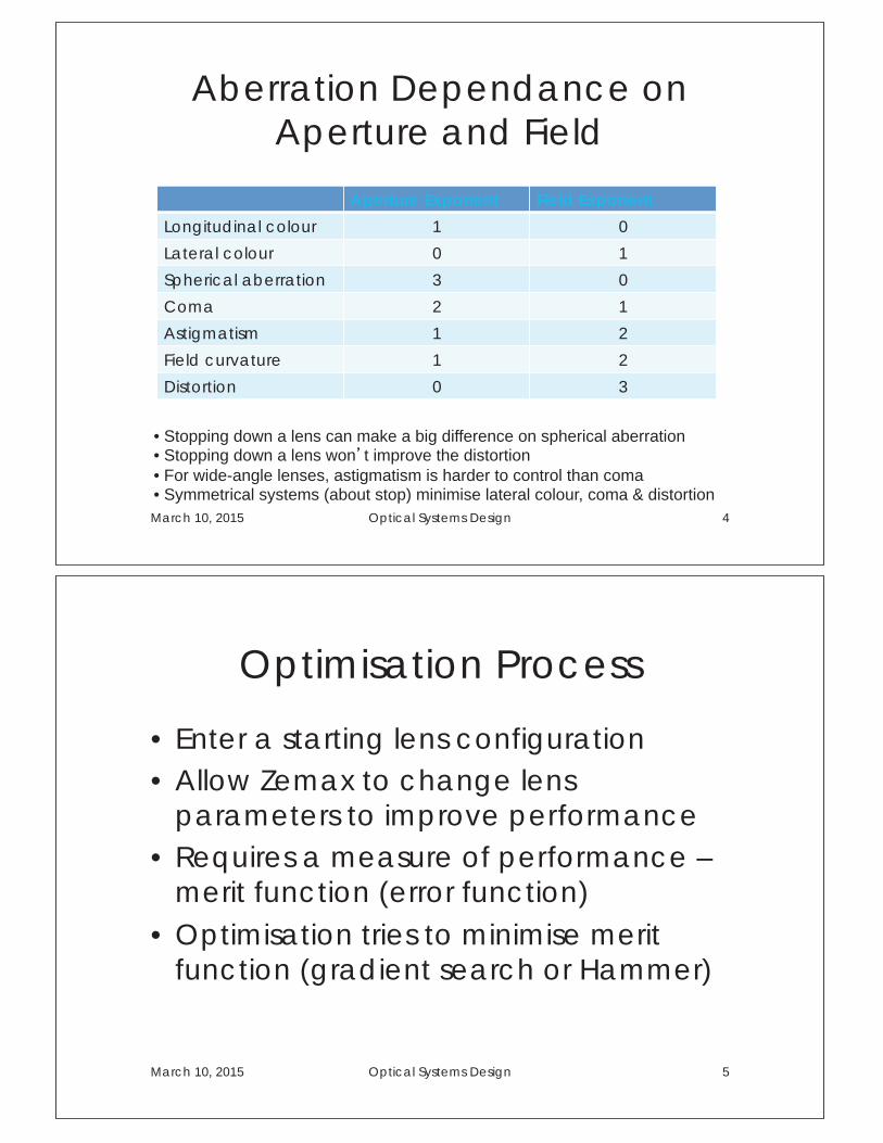
Aberration Dependance on Aperture and Field
Aperture Exponent Field Exponent
Longitudinal colour 1 0
Lateral colour 0 1
Spherical aberration 3 0
Coma 2 1
Astigmatism 1 2
Field curvature 1 2
Distortion 0 3
March 10, 2015 Optical Systems Design 4
• Stopping down a lens can make a big difference on spherical aberration • Stopping down a lens won t improve the distortion • For wide-angle lenses, astigmatism is harder to control than coma • Symmetrical systems (about stop) minimise lateral colour, coma & distortion
Optimisation Process
• Enter a starting lens configuration • Allow Zemax to change lens
parameters to improve performance • Requires a measure of performance –
merit function (error function) • Optimisation tries to minimise merit
function (gradient search or Hammer)
March 10, 2015 Optical Systems Design 5
Constituents of Merit Function
Measures of: 1. How well first-order properties are
satisfied (e.g. paraxial focus, locations of pupils and images)
2. How well special constraints are satisfied (e.g. element centre or edge thickness, curvatures, glass properties)
3. How well aberrations are controlled (e.g. image sharpness and distortion)
March 10, 2015 Optical Systems Design 6
Image Sharpness metrics
1. Spot size measured by ray-intercept errors in image plane
2. Wavefront imperfections measured by optical path difference (OPD) errors in the exit pupil
3. Modulation transfer function (MTF) in the image plane
(Start with [1], moving to [2] or [3] only in final optimisation stages)
March 10, 2015 Optical Systems Design 7
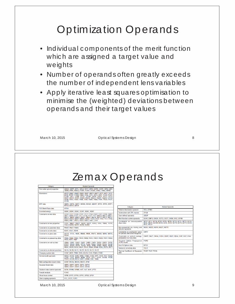
Optimization Operands
• Individual components of the merit function which are assigned a target value and weights
• Number of operands often greatly exceeds the number of independent lens variables
• Apply iterative least squares optimisation to minimise the (weighted) deviations between operands and their target values
March 10, 2015 Optical Systems Design 8
Zemax Operands
March 10, 2015 Optical Systems Design 9
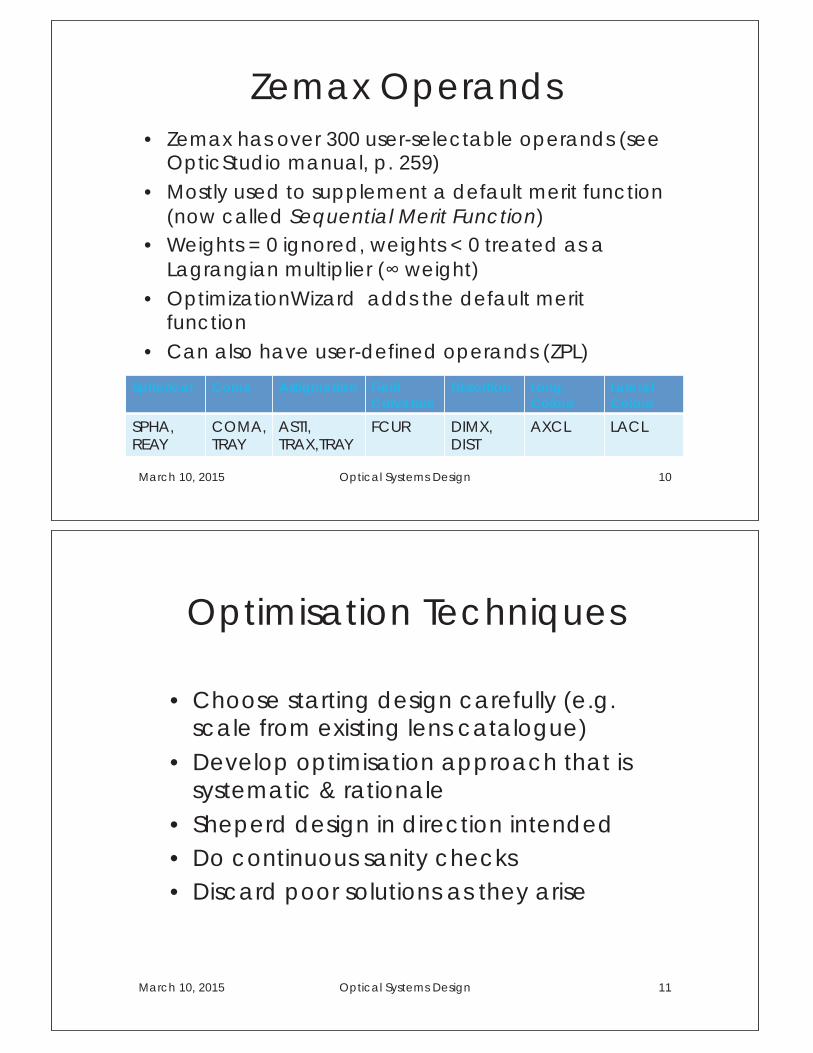
Zemax Operands • Zemax has over 300 user-selectable operands (see
OpticStudio manual, p. 259) • Mostly used to supplement a default merit function
(now called Sequential Merit Function) • Weights = 0 ignored, weights < 0 treated as a
Lagrangian multiplier (∞ weight) • OptimizationWizard adds the default merit
function • Can also have user-defined operands (ZPL)
March 10, 2015 Optical Systems Design 10
Spherical Coma Astigmatism Field Curvature
Distortion Long. Colour
Lateral Colour
SPHA, REAY
COMA, TRAY
ASTI, TRAX,TRAY
FCUR DIMX, DIST
AXCL LACL
Optimisation Techniques
• Choose starting design carefully (e.g. scale from existing lens catalogue)
• Develop optimisation approach that is systematic & rationale
• Sheperd design in direction intended • Do continuous sanity checks • Discard poor solutions as they arise
March 10, 2015 Optical Systems Design 11
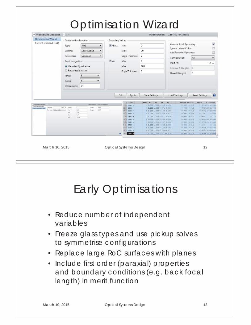
Optimisation Wizard
March 10, 2015 Optical Systems Design 12
Early Optimisations
• Reduce number of independent variables
• Freeze glass types and use pickup solves to symmetrise configurations
• Replace large RoC surfaces with planes • Include first order (paraxial) properties
and boundary conditions (e.g. back focal length) in merit function
March 10, 2015 Optical Systems Design 13
Intermediate Optimisations
• Start to control on-axis and off-axis aberrations
• Chromatic aberrations using only two extreme wavelengths
• Monochromatic aberrations using single central wavelength
• Typically: longitudinal & lateral colour, spherical & distortion
• Keep image plane at paraxial focus
March 10, 2015 Optical Systems Design 14
Final Optimisations • Shrink polychromatic spots for all field angles • Use several wavelengths across the band • Re-optimise using wavefront OPDs in exit
pupil rather than transverse ray errors (spots) on image surface
• Allow small amount of paraxial defocussing • Include any deliberate mechanical
vignetting • Take a critical look at the final lens & its
performance
March 10, 2015 Optical Systems Design 15
Potential Problem Areas
• Avoid systems which attempt to balance lenses with large amounts of positive and negative power
• Avoid highly curved surfaces and grazing rays • Look out for designs which have individual
elements which stand out as either very strong (split) or very weak (eliminate)
• Watch for variables that are only weakly effective • Avoid aspherics unless really necessary • Avoid glasses with undesirable properties (e.g. low
transmission, softness)
March 10, 2015 Optical Systems Design 16
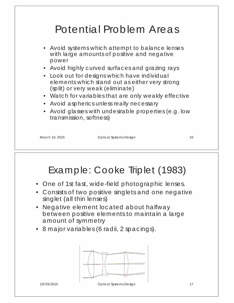
Example: Cooke Triplet (1983) • One of 1st fast, wide-field photographic lenses. • Consists of two positive singlets and one negative
singlet (all thin lenses) • Negative element located about halfway
between positive elements to maintain a large amount of symmetry
• 8 major variables (6 radii, 2 spacings).
10/03/2015 Optical Systems Design 17
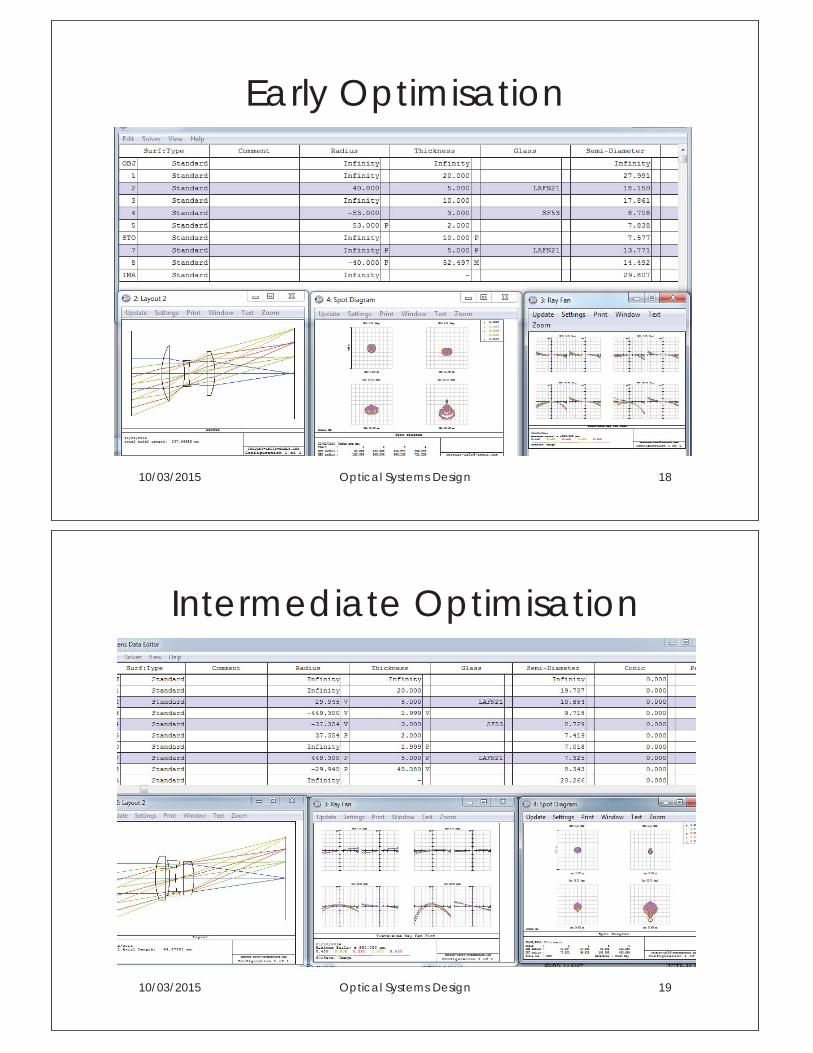
Early Optimisation
10/03/2015 Optical Systems Design 18
Intermediate Optimisation
10/03/2015 Optical Systems Design 19
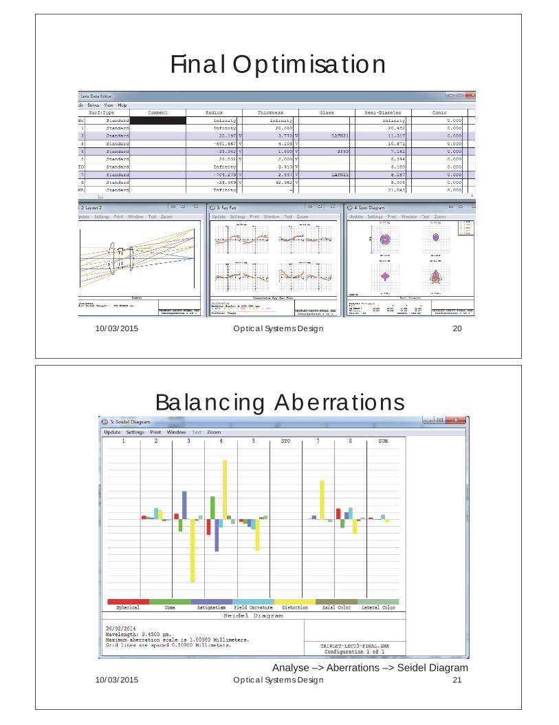
Final Optimisation
10/03/2015 Optical Systems Design 20
Balancing Aberrations
10/03/2015 Optical Systems Design 21 Analyse –> Aberrations –> Seidel Diagram
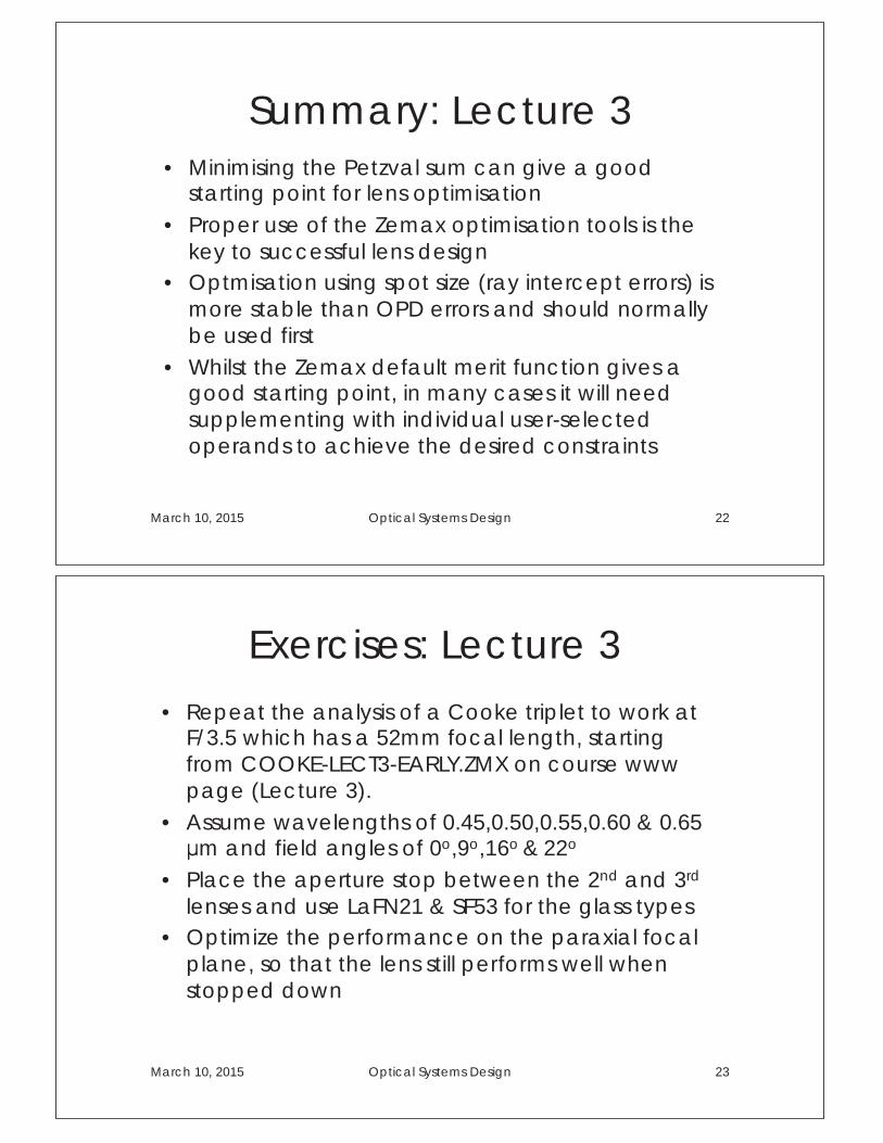
Summary: Lecture 3 • Minimising the Petzval sum can give a good
starting point for lens optimisation • Proper use of the Zemax optimisation tools is the
key to successful lens design • Optmisation using spot size (ray intercept errors) is
more stable than OPD errors and should normally be used first
• Whilst the Zemax default merit function gives a good starting point, in many cases it will need supplementing with individual user-selected operands to achieve the desired constraints
March 10, 2015 Optical Systems Design 22
Exercises: Lecture 3
• Repeat the analysis of a Cooke triplet to work at F/3.5 which has a 52mm focal length, starting from COOKE-LECT3-EARLY.ZMX on course www page (Lecture 3).
• Assume wavelengths of 0.45,0.50,0.55,0.60 & 0.65 µm and field angles of 0o,9o,16o & 22o
• Place the aperture stop between the 2nd and 3rd lenses and use LaFN21 & SF53 for the glass types
• Optimize the performance on the paraxial focal plane, so that the lens still performs well when stopped down
March 10, 2015 Optical Systems Design 23
Tolerancing in Zemax
Lecture 4
Objectives: Lecture 4
At the end of this lecture you should: 1. Understand the reason for tolerancing and
its relation to typical manufacturing errors 2. Be able to perform a Sensitivity Analysis
and Inverse Sensitivity Analysis on a new design
3. Be able to interpret the data from a Monte Carlo tolerancing analysis of a new design
March 16, 2015 Optical Systems Design 2
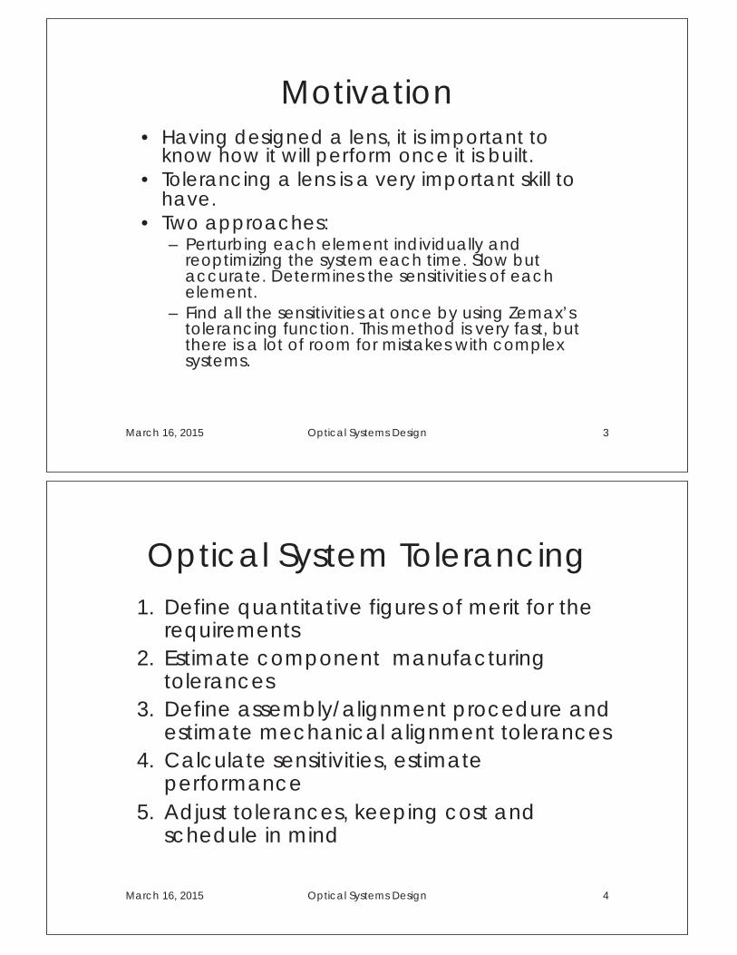
Motivation • Having designed a lens, it is important to
know how it will perform once it is built. • Tolerancing a lens is a very important skill to
have. • Two approaches:
– Perturbing each element individually and reoptimizing the system each time. Slow but accurate. Determines the sensitivities of each element.
– Find all the sensitivities at once by using Zemax’s tolerancing function. This method is very fast, but there is a lot of room for mistakes with complex systems.
March 16, 2015 Optical Systems Design 3
Optical System Tolerancing 1. Define quantitative figures of merit for the
requirements 2. Estimate component manufacturing
tolerances 3. Define assembly/alignment procedure and
estimate mechanical alignment tolerances 4. Calculate sensitivities, estimate
performance 5. Adjust tolerances, keeping cost and
schedule in mind
March 16, 2015 Optical Systems Design 4
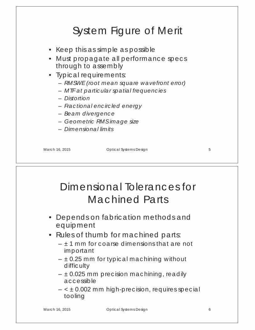
System Figure of Merit
• Keep this as simple as possible • Must propagate all performance specs
through to assembly • Typical requirements:
– RMSWE (root mean square wavefront error) – MTF at particular spatial frequencies – Distortion – Fractional encircled energy – Beam divergence – Geometric RMS image size – Dimensional limits
March 16, 2015 Optical Systems Design 5
Dimensional Tolerances for Machined Parts
• Depends on fabrication methods and equipment
• Rules of thumb for machined parts: – ± 1 mm for coarse dimensions that are not
important – ± 0.25 mm for typical machining without
difficulty – ± 0.025 mm precision machining, readily
accessible – < ± 0.002 mm high-precision, requires special
tooling
March 16, 2015 Optical Systems Design 6
Dimensional Tolerances for Optical Elements
• Diameter • Clear aperture • Thickness • Wedge Angles
– wedge or optical deviation for lenses – angles for prisms
• Bevels • Mounting surfaces
Start with nominal tolerances from lens fabricator
March 16, 2015 Optical Systems Design 7
Tolerancing Surface Shape • Specifications are based on measurement:
– Inspection with test plate: • Typical spec: 0.5 fringe
– Measurement with phase shift interferometer: • Typical spec: 0.05 λ rms
• For most diffraction-limited systems, rms surface gives a good figure of merit
• Special systems require a Power Spectral Density (PSD) spec
• Aspheric systems really need a slope spec, but this is uncommon. Typically, assume the surface irregularities follow low order forms and simulate them using Zernike polynomials
March 16, 2015 Optical Systems Design 8
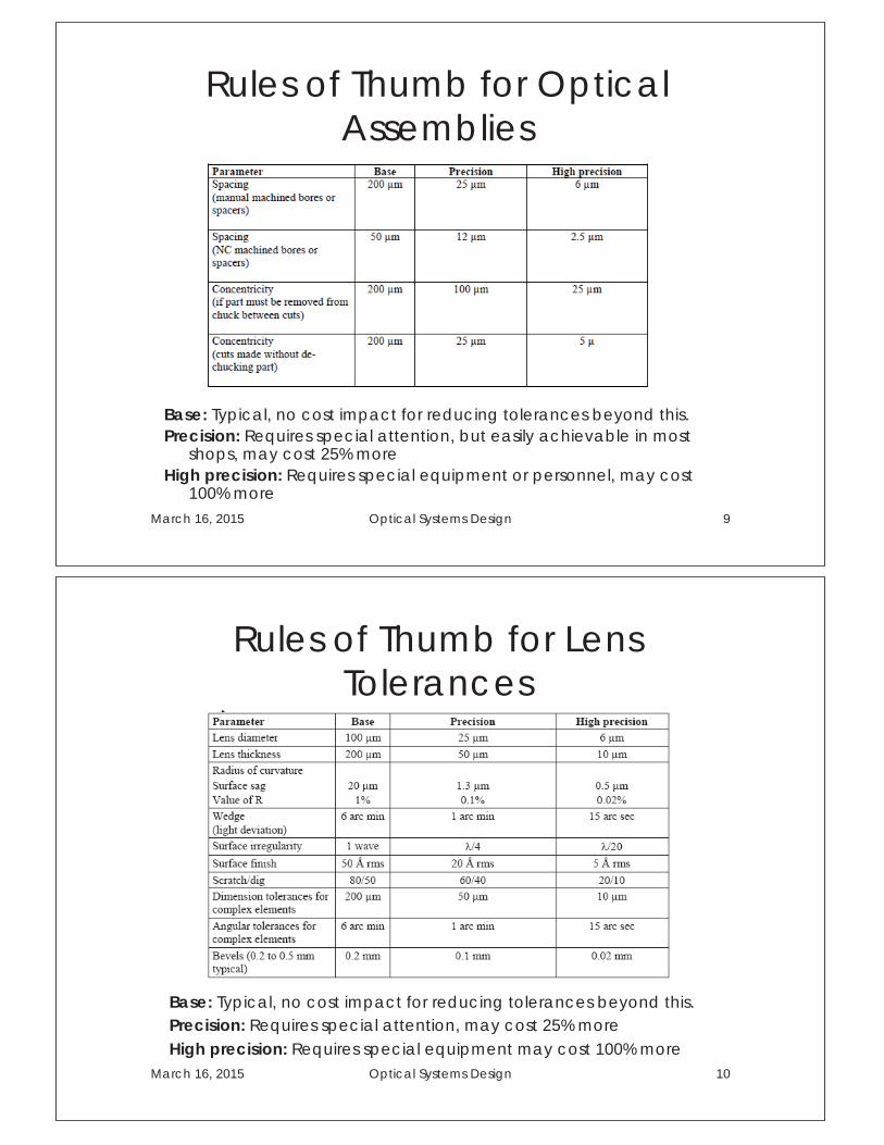
Rules of Thumb for Optical Assemblies
Base: Typical, no cost impact for reducing tolerances beyond this. Precision: Requires special attention, but easily achievable in most
shops, may cost 25% more High precision: Requires special equipment or personnel, may cost
100% more March 16, 2015 Optical Systems Design 9
Rules of Thumb for Lens Tolerances
Base: Typical, no cost impact for reducing tolerances beyond this. Precision: Requires special attention, may cost 25% more High precision: Requires special equipment may cost 100% more
March 16, 2015 Optical Systems Design 10
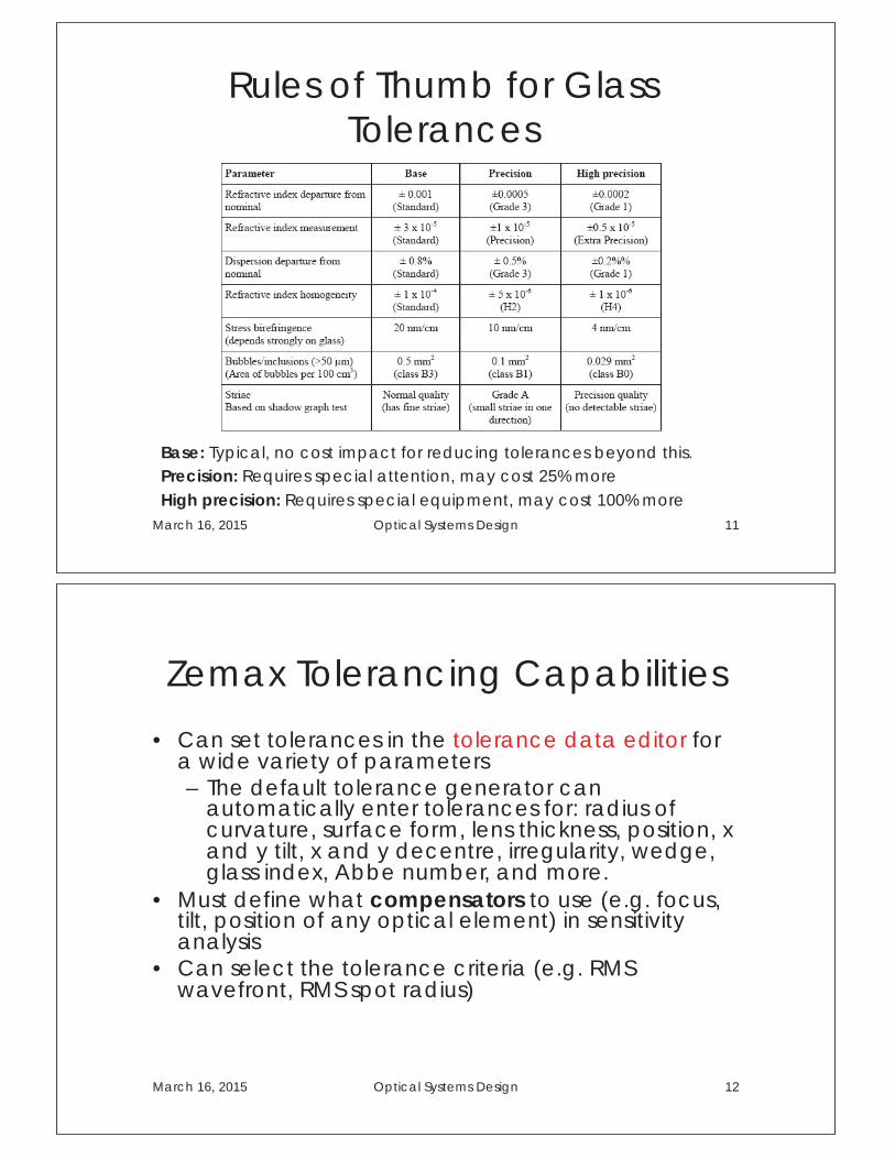
Rules of Thumb for Glass Tolerances
Base: Typical, no cost impact for reducing tolerances beyond this. Precision: Requires special attention, may cost 25% more High precision: Requires special equipment, may cost 100% more
March 16, 2015 Optical Systems Design 11
Zemax Tolerancing Capabilities
• Can set tolerances in the tolerance data editor for a wide variety of parameters – The default tolerance generator can
automatically enter tolerances for: radius of curvature, surface form, lens thickness, position, x and y tilt, x and y decentre, irregularity, wedge, glass index, Abbe number, and more.
• Must define what compensators to use (e.g. focus, tilt, position of any optical element) in sensitivity analysis
• Can select the tolerance criteria (e.g. RMS wavefront, RMS spot radius)
March 16, 2015 Optical Systems Design 12
Zemax Tolerancing Tools
• ZEMAX conducts an analysis of the tolerances using any or all of these three tools: – Sensitivity Analysis – Inverse Sensitivity Analysis – Monte Carlo Analysis
March 16, 2015 Optical Systems Design 13
I: Sensitivity Analysis
• The sensitivity analysis considers each defined tolerance sequentially (independent).
• Parameters are adjusted to the limits of the tolerance range, and then the optimum value of each compensator is determined.
• A table is generated listing the contribution of each tolerance to the performance loss.
March 16, 2015 Optical Systems Design 14
II: Inverse Sensitivity Analysis
• The inverse sensitivity analysis iteratively computes the tolerance limits on each parameter when the maximum or incremental degradation in performance is defined.
• Limits may be overall or specific to each field or configuration.
March 16, 2015 Optical Systems Design 15
III: Monte Carlo • Monte Carlo analysis is extremely powerful and useful
because all tolerances are considered at once. • Random systems are generated using the defined
tolerances. • Every parameter is randomly perturbed using
appropriate statistical models, all compensators are adjusted, and then the entire system is evaluated with all defects considered.
• User defined statistics based upon actual fabrication data is supported.
• ZEMAX can quickly simulate the fabrication of large numbers of lenses and reports statistics on simulated manufacturing yields.
March 16, 2015 Optical Systems Design 16
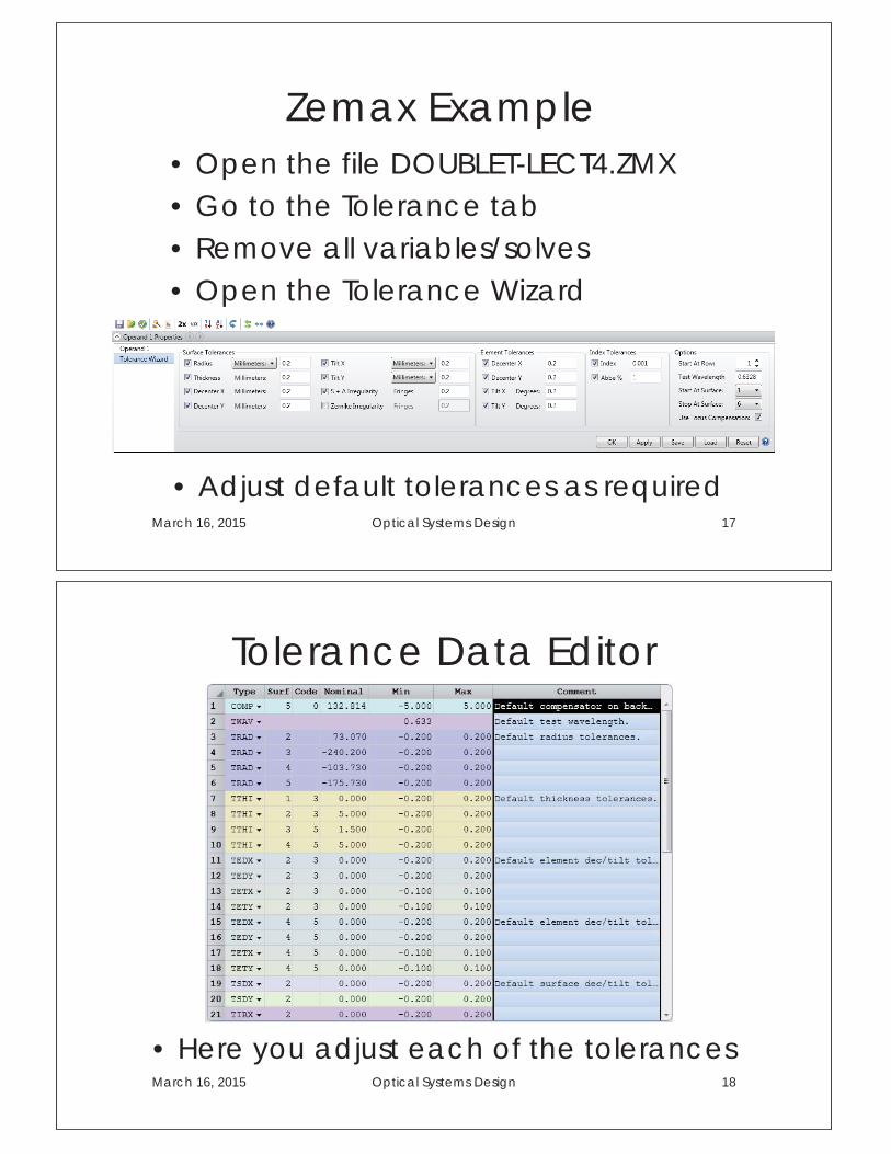
Zemax Example • Open the file DOUBLET-LECT4.ZMX • Go to the Tolerance tab • Remove all variables/solves • Open the Tolerance Wizard
March 16, 2015 Optical Systems Design 17
• Adjust default tolerances as required
Tolerance Data Editor
• Here you adjust each of the tolerances March 16, 2015 Optical Systems Design 18
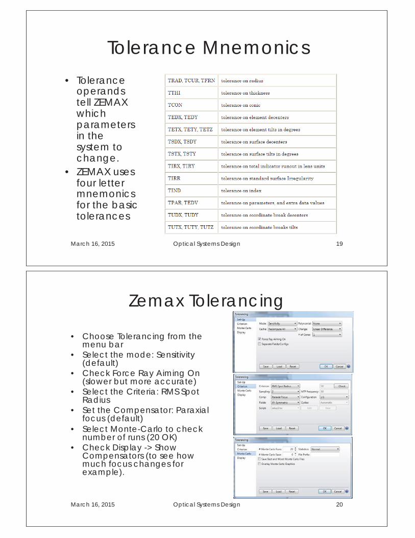
Tolerance Mnemonics
• Tolerance operands tell ZEMAX which parameters in the system to change.
• ZEMAX uses four letter mnemonics for the basic tolerances
March 16, 2015 Optical Systems Design 19
Zemax Tolerancing
• Choose Tolerancing from the menu bar
• Select the mode: Sensitivity (default)
• Check Force Ray Aiming On (slower but more accurate)
• Select the Criteria: RMS Spot Radius
• Set the Compensator: Paraxial focus (default)
• Select Monte-Carlo to check number of runs (20 OK)
• Check Display -> Show Compensators (to see how much focus changes for example).
March 16, 2015 Optical Systems Design 20
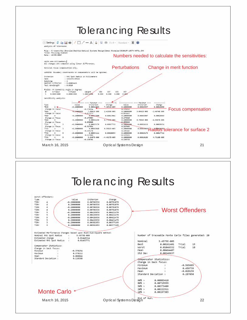
Tolerancing Results
March 16, 2015 Optical Systems Design 21
Perturbations Change in merit function
Numbers needed to calculate the sensitivities:
Focus compensation
Radius tolerance for surface 2
Tolerancing Results
March 16, 2015 Optical Systems Design 22
Worst Offenders
Monte Carlo
Summary: Lecture 4
• Tolerancing is a critical step to ensure that a lens design can be manufactured and to predict its expected performance
• Difficult because it involves complex relationships across different disciplines
• Zemax has many very powerful design tolerancing capabilities
• Important to understand how Zemax does the sensitivity analysis before you can blindly use it.
March 16, 2015 Optical Systems Design 23
Exercises: Lecture 4
• Perform tolerance analysis of the Cooke triplet lens designed in the exercise for Lecture 3
• Use precision mechanical dimensional tolerances and λ/20 RMS surface form error
• What is the mean increase in RMS spot radius from the Monte Carlo simulation ?
• Which are the three most critical dimensional tolerances ?
March 16, 2015 Optical Systems Design 24

Other Stuff
Lecture 5
Objectives: Lecture 5
At the end of this lecture you should: 1. Be aware of the Zemax capability to
approximate a lens design with catalogue components
2. Be familiar with the use of co-ordinate breaks in Zemax to model off-axis systems
3. Understand the use of non-sequential ray-tracing to model scattered light
4. Appreciate the capabilities of Zemax to model physical optics wave propagation
5. Be able to use Zemax to model the performance of imaging systems using realistic images
March 17, 2015 Optical Systems Design 2
COTS Lens Substitution • Zemax can take a custom design and substitute real
lenses • As an example start from paraxial lens model (DOUBLE-
TELECENTRIC-PARAXIAL-LECT5.ZMX) • Select Libraries -> Lens Catalogue • Use Vendor(s) drop-down menu to search standard
manufacturers catalogues • Search on lens type, EFL, pupil size • Select best match and Insert (delete paraxial surface) (DOUBLE-TELECENTRIC-EDMUNDOPTICS-LECT5.ZMX) • May need to reverse some lens elements to improve
performance, since convex surface of doublets always optimised for ∞ conjugate (there is a convenient icon above the lens data streadsheet to do this)
17/03/2015 Optical Systems Design 3
Co-ordinate Breaks • Non-axially symmetric systems where surfaces are
tilted or decentered require the use of co-ordinate breaks
• Rotate/shift local co-ordinate frame • Positive rotation (in ZEMAX) is clockwise as viewed
along +ve axis direction • Subsequent co-ordinate breaks refer to the newly
defined axis orientations • If a co-ordinate break is placed immediately before
an optical surface, it can be useful to put another one with opposite sign immediately after, thus undoing the tilt etc
• There are now simple tools in the Lens Data icon bar to tilt/decentre surfaces and add fold mirrors
March 17, 2015 Optical Systems Design 4
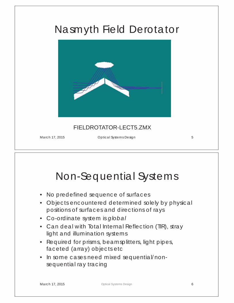
Nasmyth Field Derotator
March 17, 2015 Optical Systems Design 5
FIELDROTATOR-LECT5.ZMX
Non-Sequential Systems
• No predefined sequence of surfaces • Objects encountered determined solely by physical
positions of surfaces and directions of rays • Co-ordinate system is global • Can deal with Total Internal Reflection (TIR), stray
light and illumination systems • Required for prisms, beamsplitters, light pipes,
faceted (array) objects etc • In some cases need mixed sequential/non-
sequential ray tracing
March 17, 2015 Optical Systems Design 6
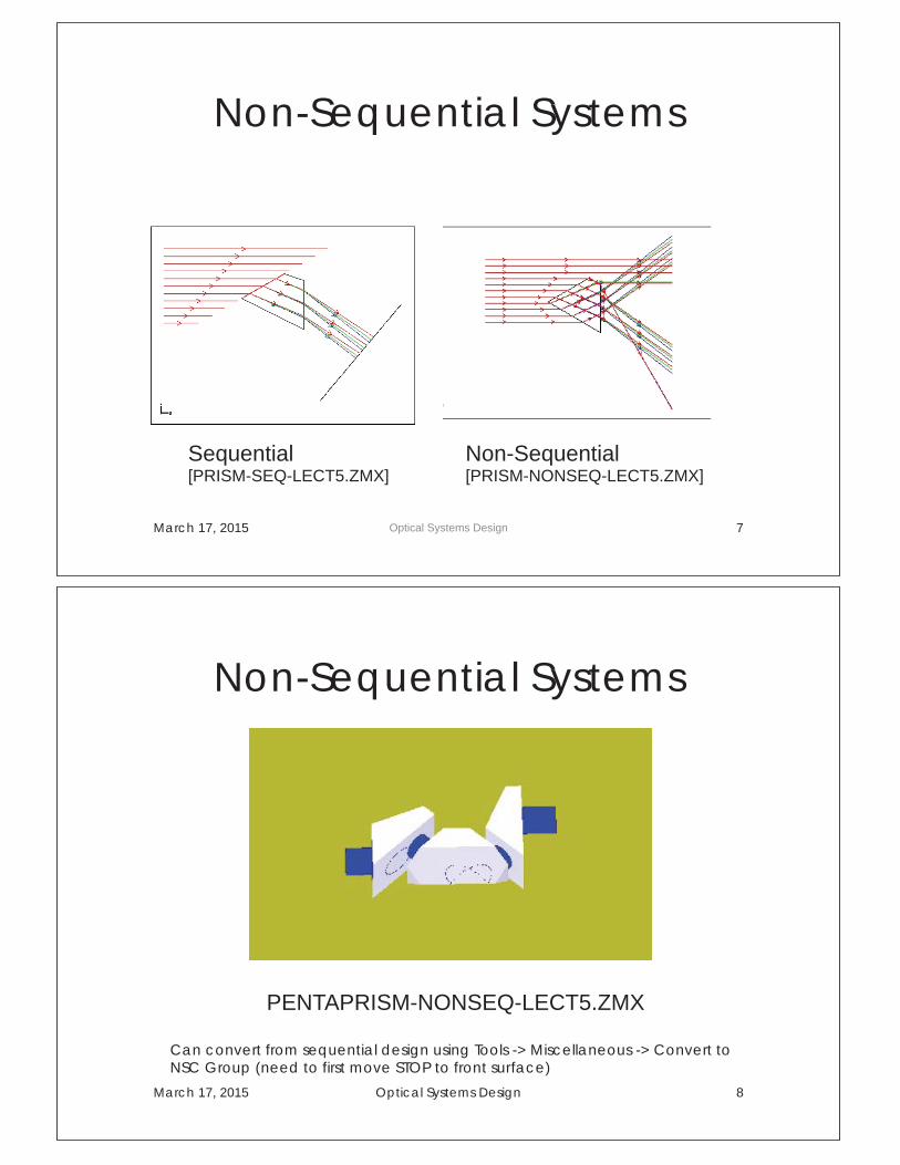
Non-Sequential Systems
March 17, 2015 Optical Systems Design 7
Sequential [PRISM-SEQ-LECT5.ZMX]
Non-Sequential [PRISM-NONSEQ-LECT5.ZMX]
Non-Sequential Systems
March 17, 2015 Optical Systems Design 8
PENTAPRISM-NONSEQ-LECT5.ZMX
Can convert from sequential design using Tools -> Miscellaneous -> Convert to NSC Group (need to first move STOP to front surface)
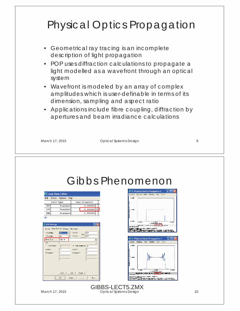
Physical Optics Propagation
• Geometrical ray tracing is an incomplete description of light propagation
• POP uses diffraction calculations to propagate a light modelled as a wavefront through an optical system
• Wavefront is modeled by an array of complex amplitudes which is user-definable in terms of its dimension, sampling and aspect ratio
• Applications include fibre coupling, diffraction by apertures and beam irradiance calculations
March 17, 2015 Optical Systems Design 9
Gibbs Phenomenon
March 17, 2015 Optical Systems Design 10 GIBBS-LECT5.ZMX
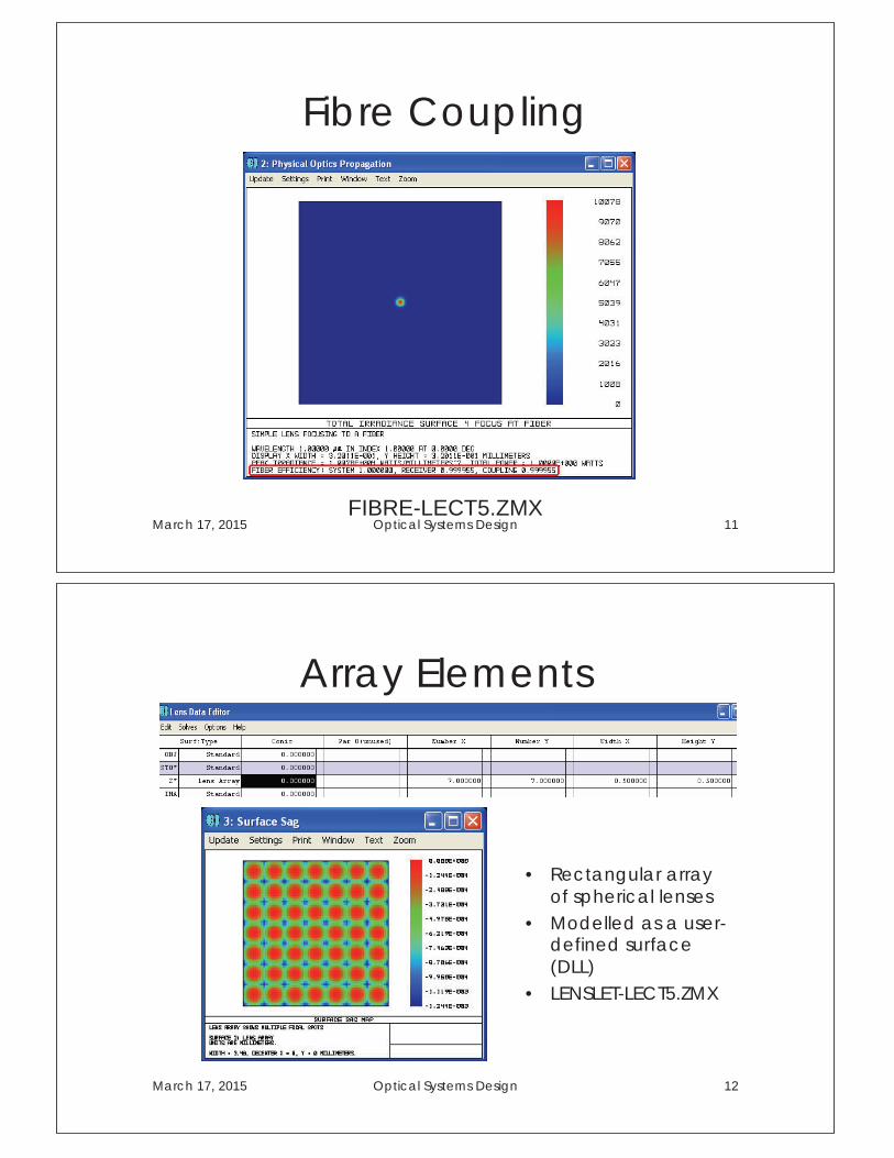
Fibre Coupling
March 17, 2015 Optical Systems Design 11 FIBRE-LECT5.ZMX
Array Elements
• Rectangular array of spherical lenses
• Modelled as a user-defined surface (DLL)
• LENSLET-LECT5.ZMX
March 17, 2015 Optical Systems Design 12
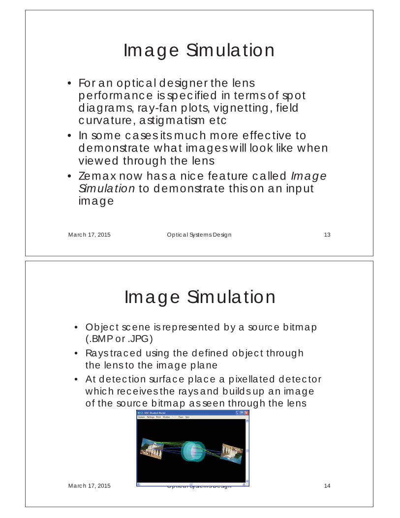
Image Simulation
• For an optical designer the lens performance is specified in terms of spot diagrams, ray-fan plots, vignetting, field curvature, astigmatism etc
• In some cases its much more effective to demonstrate what images will look like when viewed through the lens
• Zemax now has a nice feature called Image Simulation to demonstrate this on an input image
March 17, 2015 Optical Systems Design 13
Image Simulation
• Object scene is represented by a source bitmap (.BMP or .JPG)
• Rays traced using the defined object through the lens to the image plane
• At detection surface place a pixellated detector which receives the rays and builds up an image of the source bitmap as seen through the lens
March 17, 2015 Optical Systems Design 14
Design for Fabrication
• Primary considerations: optical material, component size, shape, and manufacturing tolerances
• Minimize cost and delivery time by using COTS items whenever possible
• Minimize risk through prototyping and pre-production models
March 17, 2015 Optical Systems Design 15
Optical Materials • Over 100 optical glasses available worldwide • Each manufacturer has a list of “preferred” glasses that are
most frequently melted and usually available from stock • Generally can substitute similar glasses from different
manufacturers (and re-optimise) • Material quality defined by tolerances on spectral transmission,
index of refraction, dispersion, striae grades (AA/A/B), homogeneity (H1-H4), and birefringence (NSK/NSSK)
• Tighter than standard optical tolerances require additional cost and time
• May be more economical to add a lens to the design in order to avoid expensive glasses
• Some glasses (e.g. SF-59) made much less frequently than others (e.g. BK-7)
March 17, 2015 Optical Systems Design 16
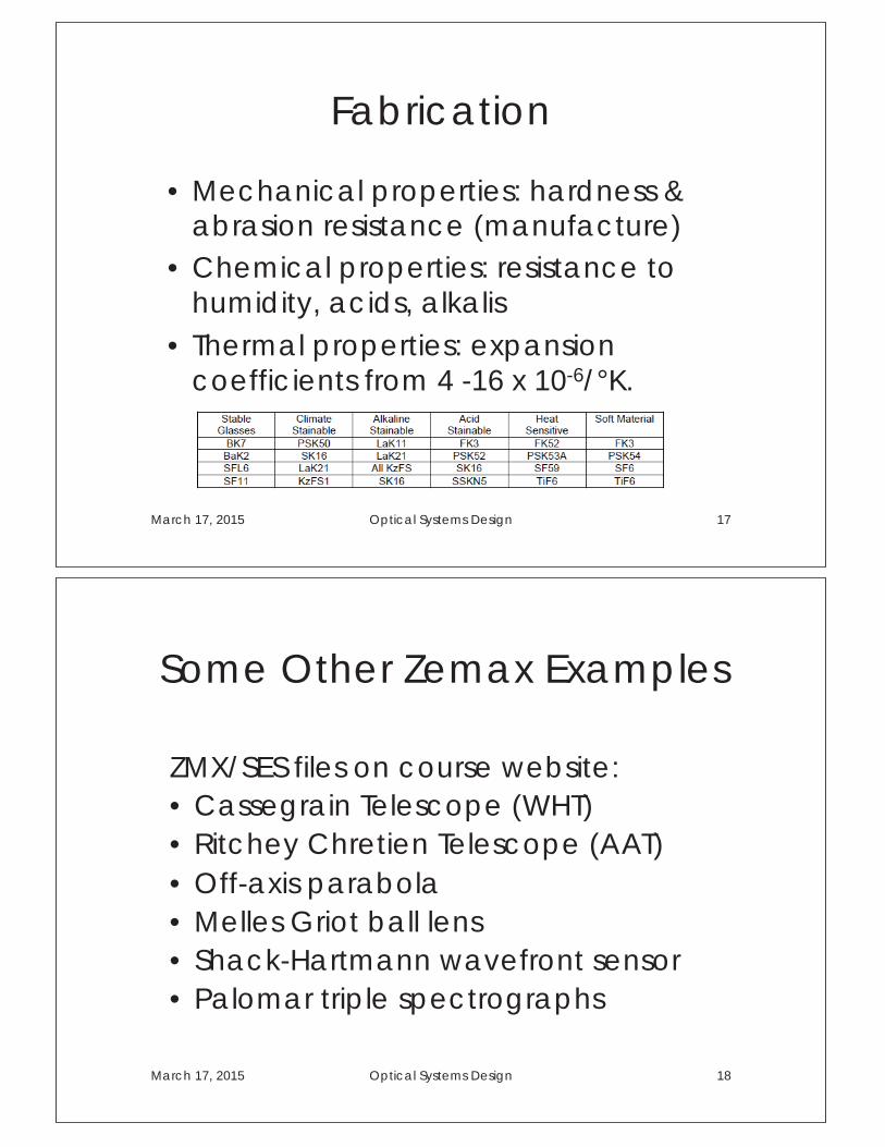
Fabrication
• Mechanical properties: hardness & abrasion resistance (manufacture)
• Chemical properties: resistance to humidity, acids, alkalis
• Thermal properties: expansion coefficients from 4 -16 x 10-6/°K.
March 17, 2015 Optical Systems Design 17
Some Other Zemax Examples
ZMX/SES files on course website: • Cassegrain Telescope (WHT) • Ritchey Chretien Telescope (AAT) • Off-axis parabola • Melles Griot ball lens • Shack-Hartmann wavefront sensor • Palomar triple spectrographs
March 17, 2015 Optical Systems Design 18
Summary: Lecture 5 • Co-ordinate breaks allow Zemax to model
arbitrarily complex off-axis systems in a local co-ordinate system
• Need care in use to avoid over-complication • Non-sequential mode allows complex objects to
be defined using a global co-ordinate system • Can also be used to model scattered light and
illumination systems • Physical optics propagation in Zemax includes the
effects of diffraction • Fabrication issues need to be thought about early
in the instrument design phase
March 17, 2015 Optical Systems Design 19
Exercises: Lecture 5
• Work your way through some of the example Zemax files, evaluating their performance and making sure that you understand the prescription data.
March 17, 2015 Optical Systems Design 20

Homework Problem • Design a very simple telephoto lens with the following
first-order properties:
• Design goal: maintain all first-order properties and achieve rms spot sizes ≤ 20 μm. Start from two paraxial lenses with focal lengths 75mm and -75mm.
• Final solutions should include a layout diagram, spot diagram and system prescription data (also email the Zemax file).
• Hand in the solutions to my pigeon hole by Friday 17th April.
17/03/2015 Optical Systems Design 21
μ