Optical Spectroscopy

Introduction & Overview

Ian Browne & Chris O’Dea

Acknowledgements: Jerry Kriss & Jeff Valenti

Aims for this lecture

What is Spectroscopy? Spectrographs Information in a Spectrum

• Emission Lines

• Absorption Lines

Astrophysical Results from Spectroscopy

What is Spectroscopy?

Spectroscopy is the study of radiation that has been dispersed into its component wavelengths.

First astronomical spectrum—the Sun (Newton 1666; Wollaston 1802; Fraunhofer 1814, 1817).

A picture may be worth a thousand words,but a spectrum is worth a thousand pictures.

—Blair Savage

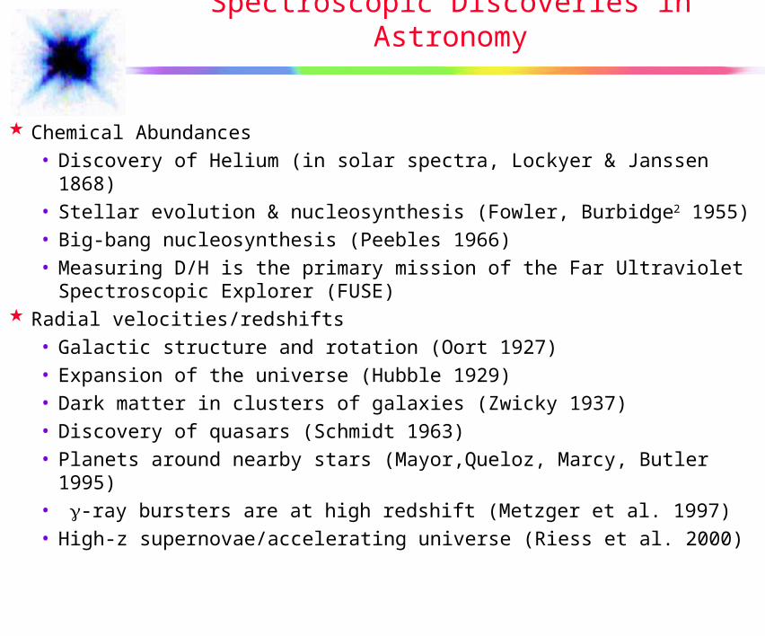
Spectroscopic Discoveries in Astronomy

Chemical Abundances• Discovery of Helium (in solar spectra, Lockyer & Janssen 1868)• Stellar evolution & nucleosynthesis (Fowler, Burbidge2 1955)• Big-bang nucleosynthesis (Peebles 1966)• Measuring D/H is the primary mission of the Far Ultraviolet

Spectroscopic Explorer (FUSE) Radial velocities/redshifts

• Galactic structure and rotation (Oort 1927)• Expansion of the universe (Hubble 1929)• Dark matter in clusters of galaxies (Zwicky 1937)• Discovery of quasars (Schmidt 1963)• Planets around nearby stars (Mayor,Queloz, Marcy, Butler 1995)• -ray bursters are at high redshift (Metzger et al. 1997)• High-z supernovae/accelerating universe (Riess et al. 2000)

Spectroscopic Discoveries in Astronomy

Line Widths• Stellar surface gravities (white dwarfs)• Stellar rotation (Schlesinger 1909)• Velocity dispersions in ellipticals and bulges

• Ellipticals are not rotationally supported (Illingworth 1977; Schechter & Gunn 1979)

• Black holes in galactic nuclei (e.g., Kormendy & Richstone 1995)

What are those Squiggly Lines?

Spectroscopic observations rarely receive press attention since the results aren’t as photogenic or as easily understood as astronomical images:• 2 of 32 HST press releases during 2000 were based on

spectroscopic observations.• Neither shows a spectrum!

Some exceptions:• Black hole in M87, FOS & WFPC2 (Ford, Harms, et al. 1994)• He II in the IGM, HUT (Davidsen, Kriss, Zheng 1996)• Black hole in M84, STIS (Bower et al. 1997)• SN1987A, STIS (Sonneborn et al. 1997)

Kinds of Spectrographs

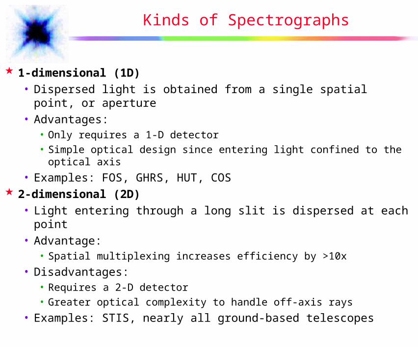
1-dimensional (1D)• Dispersed light is obtained from a single spatial point, or

aperture• Advantages:

• Only requires a 1-D detector

• Simple optical design since entering light confined to the optical axis

• Examples: FOS, GHRS, HUT, COS 2-dimensional (2D)

• Light entering through a long slit is dispersed at each point• Advantage:

• Spatial multiplexing increases efficiency by >10x

• Disadvantages:• Requires a 2-D detector

• Greater optical complexity to handle off-axis rays

• Examples: STIS, nearly all ground-based telescopes

Kinds of Spectrographs

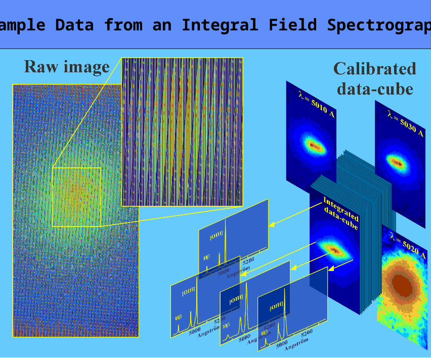
3-dimensional (3D)—Integral Field Spectrographs• An entire area of the sky is imaged, and light from each pixel is

separately dispersed into a spectrum. From this one can construct “data cubes” giving intensity as a function of (x, y).

• For compact objects, multiplexing the additional spatial element provides another order of magnitude increase in efficiency.

(The tradeoff is the size of the field covered.)• Examples:

• Lenslet arrays: TIGER, OASIS (CFHT)

• Fiber arrays: DensePack (KPNO, retired), INTEGRAL (WHT)

• Image slicers: popular for IR applications, MPE’s “3D”

• Fabry-Perot interferometers: Rutgers (CTIO), TAURUS-2 (AAT)

The OASIS Integral Field Spectrograph at the CFHT

Sample Data from an Integral Field Spectrograph

Atmospheric Transmission (300-1100 nm)

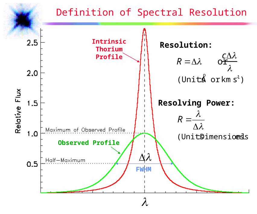
Definition of Spectral Resolution

IntrinsicThoriumProfile

Observed Profile

FWHM

Resolution:

R or c

)s kmor A :(Units 1-o

Resolving Power:

R

ess)Dimensionl :(Units

Morphological Features in Spectra

EmissionLines

AbsorptionLines

Continuum Fit

Continuum

Line Flux F d

1

2

)cm s erg :(Units -2-1

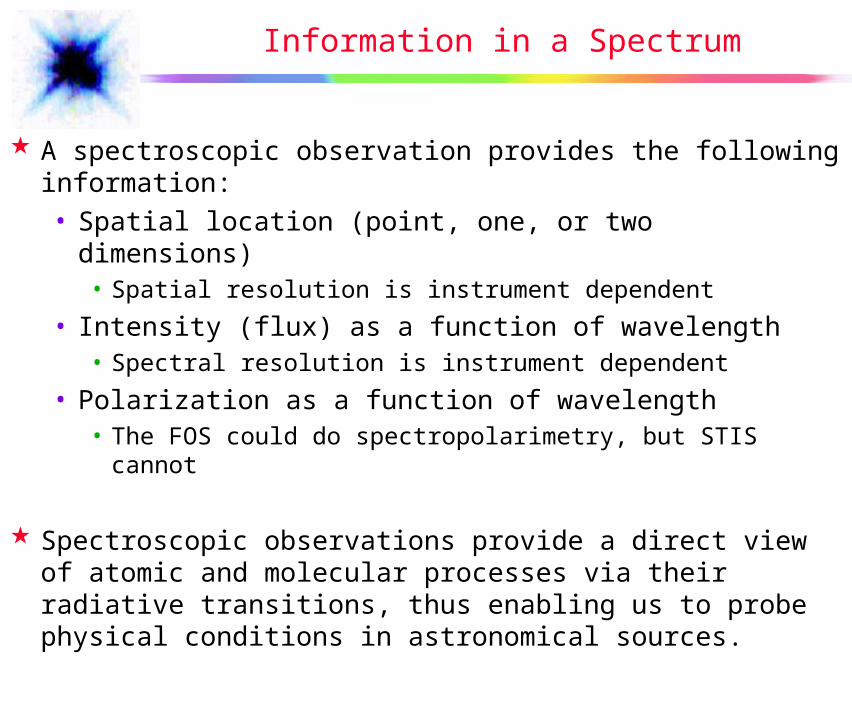
Information in a Spectrum

A spectroscopic observation provides the following information:• Spatial location (point, one, or two dimensions)

• Spatial resolution is instrument dependent

• Intensity (flux) as a function of wavelength• Spectral resolution is instrument dependent

• Polarization as a function of wavelength• The FOS could do spectropolarimetry, but STIS cannot

Spectroscopic observations provide a direct view of atomic and molecular processes via their radiative transitions, thus enabling us to probe physical conditions in astronomical sources.

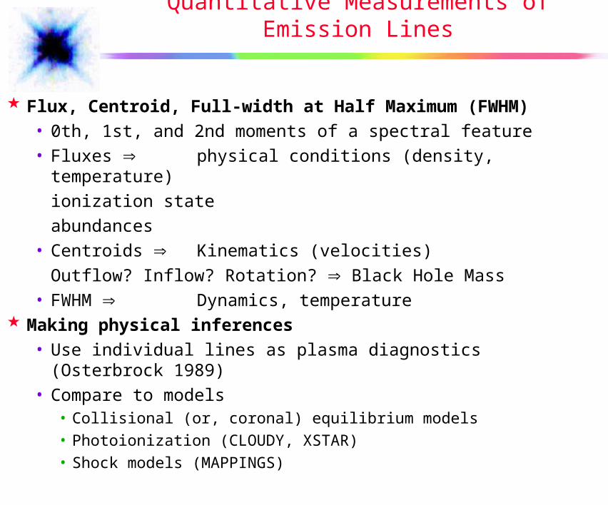
Quantitative Measurements of Emission Lines

Flux, Centroid, Full-width at Half Maximum (FWHM)• 0th, 1st, and 2nd moments of a spectral feature• Fluxes physical conditions (density, temperature)

ionization state

abundances• Centroids Kinematics (velocities)

Outflow? Inflow? Rotation? Black Hole Mass

• FWHM Dynamics, temperature Making physical inferences

• Use individual lines as plasma diagnostics (Osterbrock 1989)• Compare to models

• Collisional (or, coronal) equilibrium models• Photoionization (CLOUDY, XSTAR)• Shock models (MAPPINGS)

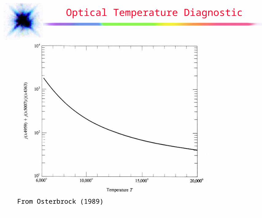
Optical Temperature Diagnostic

From Osterbrock (1989)

Optical Density Diagnostics

From Osterbrock (1989)

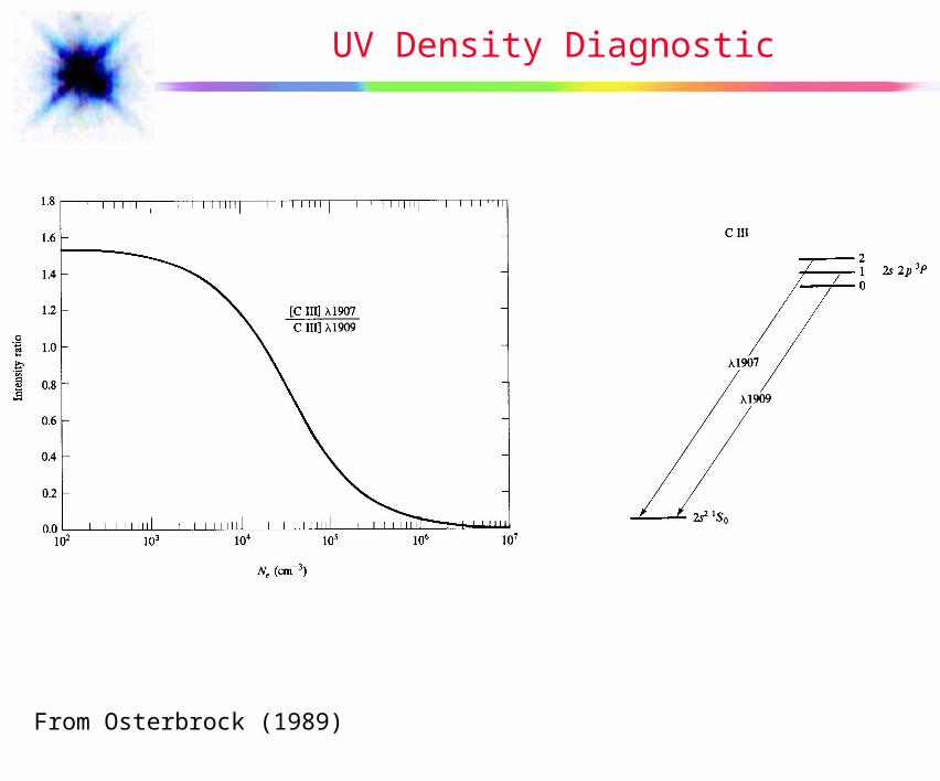
UV Density Diagnostic

From Osterbrock (1989)

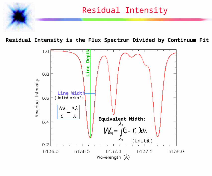
Residual Intensity

Residual Intensity is the Flux Spectrum Divided by Continuum Fit

Line WidthL

ine

Dep

th

km/s) or A :(Unitso

c

v

eqW 1 r 1

2 d

Equivalent Width:

)A :(Unitso

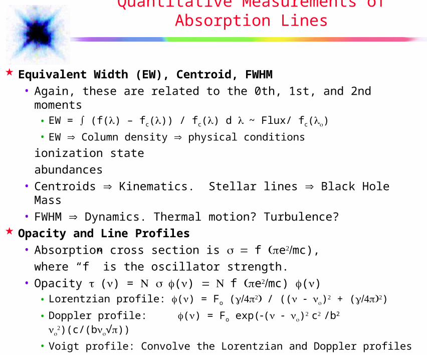
Quantitative Measurements of Absorption Lines

Equivalent Width (EW), Centroid, FWHM• Again, these are related to the 0th, 1st, and 2nd moments

• EW = ∫(f() – fc()) / fc() d ~ Flux/ fc()

• EW Column density physical conditions

ionization state

abundances• Centroids Kinematics. Stellar lines Black Hole Mass• FWHM Dynamics. Thermal motion? Turbulence?

Opacity and Line Profiles• Absorption cross section is f emc),

where “f” is the oscillator strength.• Opacity () = () f emc) ()

• Lorentzian profile: () = Fo (/ (( ) + ()

• Doppler profile: () = Fo exp(( )c/b2 )(c/(b√))

• Voigt profile: Convolve the Lorentzian and Doppler profiles

Absorption Line Profiles

Doppler

Lorentzian

Curves of Growth

Curve of growth for the line equivalent width is

W = ∫ ( e) d

Linear portion: W / ~ Nf

Flat portion: W / ~ ln(Nf

Square-root portion: W / ~ (Nf

Spectral Features due to Hydrogen

Ultra-deep Echelle Spectra of the Orion Nebula

Region of the Balmer limit. Hydrogen lines up to n=28 are detected.

Emission lines of OII multiplet line 1 and very week NIII and NII lines

Baldwin etal 2000, ApJS, 129, 229

Measuring the Mass of Black Holes in Galaxies

Use stellar motions (rotation and velocity dispersion) to constrain models of stellar orbit distributions in the potential of a galaxy plus a central supermassive black hole (e.g., van der Marel et al. 1997).

When gas disks are present, rotational velocities can be measured using line emission from the gas. Model as Keplerian rotation in the potential of the galaxy plus a central supermassive black hole (e.g., Harms et al. 1994).

Ford et al. (1994); Harms et al. (1994)

Model for Disk Velocities in M87

Courtesy L. Dressel

STIS Observations of the LINER NGC 3998

STIS Long-Slit Spectrum of NGC 3998

L. Dressel/STScI

Fitting the H+[N II] and [S II] Emission Lines

Courtesy L. DresselWavelength (Å)

Flu

x

Rotation Curve of NGC 3998

Courtesy L. Dressel

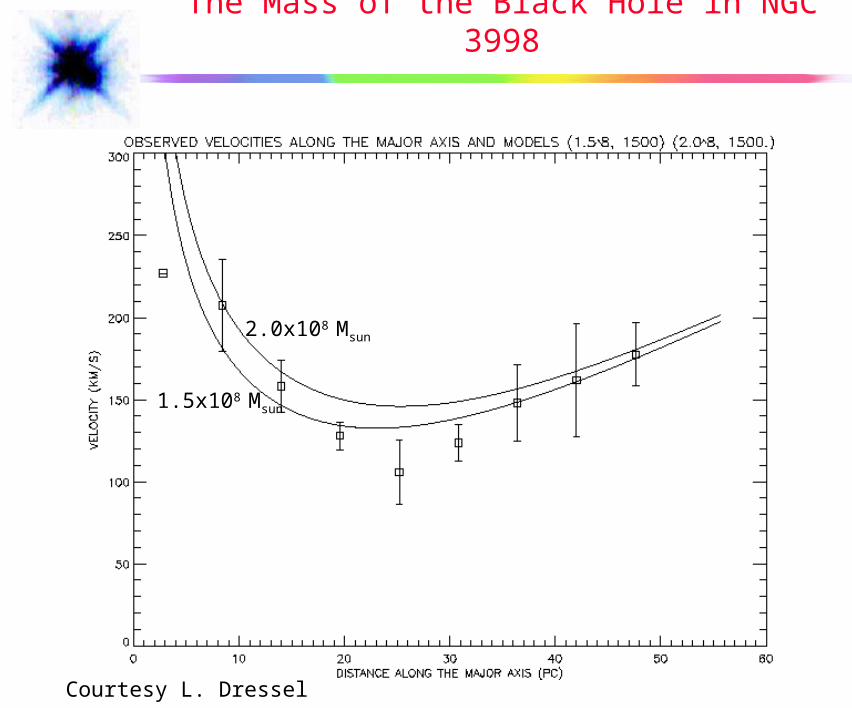
The Mass of the Black Hole in NGC 3998

Courtesy L. Dressel

2.0x108 Msun

1.5x108 Msun

BH Mass vs. Galaxy Bulge Mass

There is a relationship between BH mass and bulge luminosity. And an even tighter relationship with the bulge velocity dispersion. M(BH) ~ 10-3 M(Bulge). Ferrarese & Merritt 2000, ApJ, 539, L9

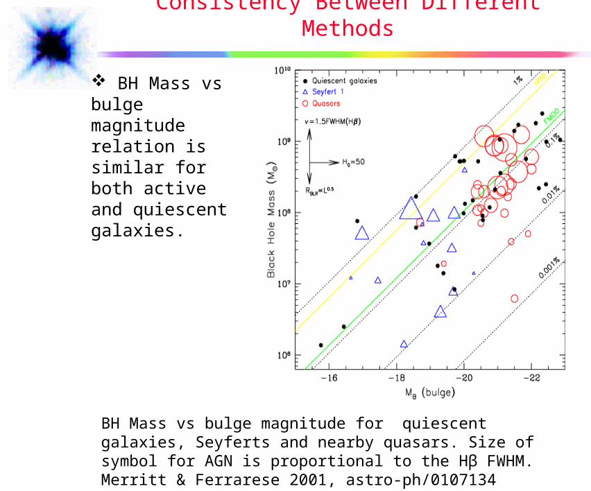
Consistency Between Different Methods

BH Mass vs bulge magnitude relation is similar for both active and quiescent galaxies.

BH Mass vs bulge magnitude for quiescent galaxies, Seyferts and nearby quasars. Size of symbol for AGN is proportional to the Hβ FWHM. Merritt & Ferrarese 2001, astro-ph/0107134

Seyfert 1

The Structure of AGN

Torus

Seyfert 2

Central Engine:Accretion Disk+Black Hole

Broad Line Region

Narrow Line Region

The AGN Paradigm

Annotated by M. Voit

Radio Luminosity – Optical Line Correlation.

There is a strong correlation between radio luminosity and optical emission line luminosity for both RL and RQ objects. (see also Baum & Heckman 1989)

Xu etal 1999, AJ, 118, 1169

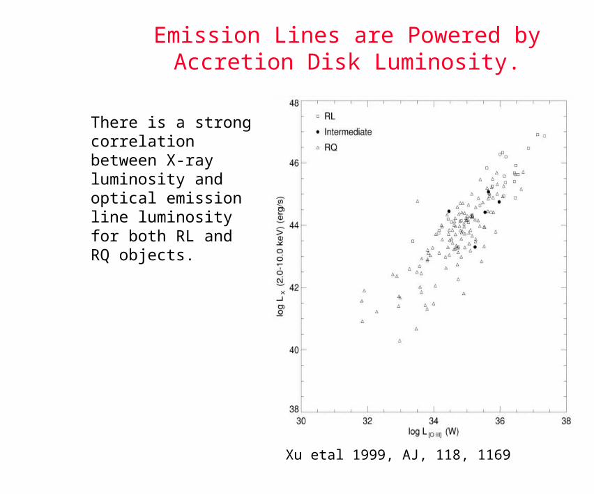
Emission Lines are Powered by Accretion Disk Luminosity.

There is a strong correlation between X-ray luminosity and optical emission line luminosity for both RL and RQ objects.

Xu etal 1999, AJ, 118, 1169

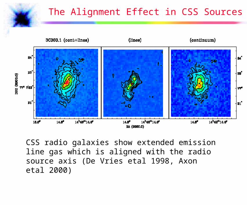
The Alignment Effect in CSS Sources

CSS radio galaxies show extended emission line gas which is aligned with the radio source axis (De Vries etal 1998, Axon etal 2000)

The Alignment Effect in CSS Sources

The emission line gas is more strongly aligned in the CSS radio galaxies than in high redshift radio galaxies.

Histogram of difference in radio and optical position angle. De Vries etal 1999, ApJ, 526, 27

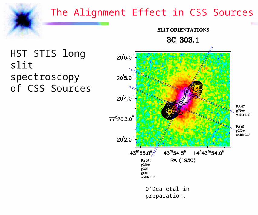
The Alignment Effect in CSS Sources

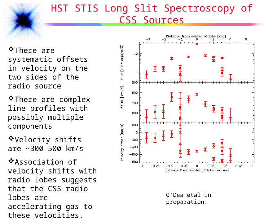
HST STIS long slit spectroscopy of CSS Sources

O’Dea etal in preparation.

HST STIS Long Slit Spectroscopy of CSS Sources

Distance along slit

O’Dea etal in preparation.

Wavelength (Velocity)

HST STIS Long Slit Spectroscopy of CSS Sources

There are systematic offsets in velocity on the two sides of the radio source

There are complex line profiles with possibly multiple components

Velocity shifts are ~300-500 km/s

Association of velocity shifts with radio lobes suggests that the CSS radio lobes are accelerating gas to these velocities.

O’Dea etal in preparation.

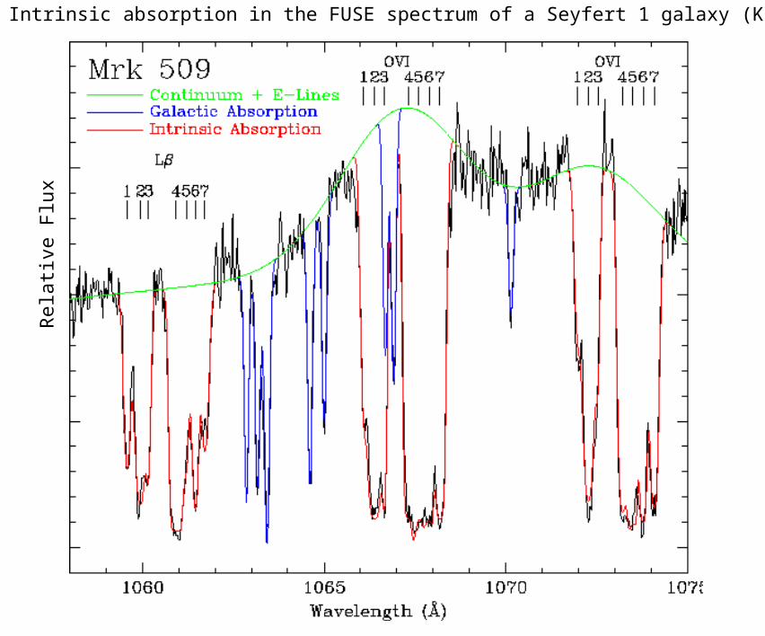
Intrinsic absorption in the FUSE spectrum of a Seyfert 1 galaxy (Kriss et al. 2000).

Rel

ativ

e F

lux

Physical Properties of the Absorbers in Mrk 509

Component#

v(km s–1)

NOVI/NHI log Ntot log U

1 –438 0.37 18.3 –1.64

2 –349 1.51 18.8 –1.19

3 –280 0.48 18.3 –1.79

4 –75 0.19 19.2 –1.73

5 –5 13.9 20.7 –0.43

6 +71 2.14 18.9 –1.41

7 +166 2.76 18.8 –1.46

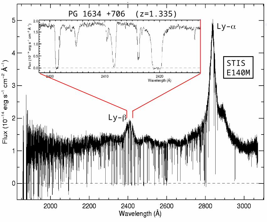
PG 1634 +706 (z=1.335)

Ly–

Ly–

STISE140M

He II in the Intergalactic Medium

Optical depth to H I ina Standard Cold Dark Matter

Model at z = 2.336

Optical depth to He II

From Croft et al. (1997)

Ford et al. (1994); Harms et al. (1994)

Supermassive Black Hole:

STIS SlitNucleus

+400 km/s

– 400 km/s

16 pc

M = 310 Msun8

References

Allen 2000, Allen’s Astrophysical Quantities, ed. A. Cox, (Springer: New York) Bower et al. 1997, ApJ, 492, L111 Croft et al. 1997, ApJ, 488, 532 Davidsen, Kriss, & Zheng 1996, Nature, 380, 47 Ford et al. 1994, ApJ, 435, L27 Fowler, Burbidge, & Burbidge 1955, ApJ, 122, 271 Fraunhofer 1817, Denkschriften der Münchner Akademie der Wissenschaften, 5, 193 Harms et al. 1994, ApJ, 435, L35 Hubble 1929, Proceedings of the National Academy of Sciences, 15, 171 Hubble & Humason 1931, ApJ, 74, 43 Illingworth 1977, ApJ, 218, L43 Kormendy & Richstone 1995, ARAA, 33, 581 Kriss et al. 2000, ApJ, 538, L17 Lockyer & Janssen 1868. See http://ww.hao.ucar.edu/public/education/sp/images/lockyer.html Mayor & Queloz 1995, Nature, 378, 355 Marcy & Butler 1995, ApJ, 464, L147 Metzger et al. 1997, Nature, 387, 878 Osterbrock 1989, Astrophysics of Gaseous Nebulae and Active Galactic Nuclei, (University Science Books: Mill Valley) Oort 1927, Bull. Astron. Inst. Netherlands, 3, 275 Peebles 1966, ApJ, 146, 542 Riess 2000, PASP, 112, 1284 Schechter & Gunn 1979, ApJ, 229, 472 Schmidt 1963, Nature, 197, 1040 Schlesinger 1909, Pub. Allegheny Obs., 1, 125 Sonneborn et al. 1997, ApJ, 492, L139 Spitzer 1978, Physical Processes in the Interstellar Medium, (Wiley: New York) Wollaston 1802, Phil. Trans. R. Soc., 92, 365 van der Marel et al. 1997, Nature, 385, 610 Zwicky 1937, ApJ, 86, 217

The End