Embed Size (px)
Citation preview


116
Advances in Biochemical Engineering/Biotechnology
Series Editor: T. Scheper
Editorial Board:W. Babel · I. Endo · S.-O. Enfors · M. Hoare · W.-S. HuB. Mattiasson · J. Nielsen · G. StephanopoulosU. von Stockar · G. T. Tsao · R. Ulber · J.-J. Zhong

Advances in Biochemical Engineering/BiotechnologySeries Editor: T. Scheper
Recently Published and Forthcoming Volumes
Optical Sensor Systems in BiotechnologyVolume Editor: Rao, G.Vol. 116, 2009
Disposable BioreactorsVolume Editor: Eibl, R., Eibl, D.Vol. 115, 2009
Engineering of Stem CellsVolume Editor: Martin, U.Vol. 114, 2009
Biotechnology in China IFrom Bioreaction to Bioseparation and BioremediationVolume Editors: Zhong, J.J., Bai, F.-W., Zhang, W.Vol. 113, 2009
Bioreactor Systems for Tissue EngineeringVolume Editors: Kasper, C., van Griensven, M.,Poertner, R.Vol. 112, 2008
Food BiotechnologyVolume Editors: Stahl, U., Donalies, U. E. B.,Nevoigt, E.Vol. 111, 2008
Protein – Protein InteractionVolume Editors: Seitz, H., Werther, M.Vol. 110, 2008
Biosensing for the 21st CenturyVolume Editors: Renneberg, R., Lisdat, F.Vol. 109, 2007
BiofuelsVolume Editor: Olsson, L.Vol. 108, 2007
Green Gene TechnologyResearch in an Area of Social ConflictVolume Editors: Fiechter, A., Sautter, C.Vol. 107, 2007
White BiotechnologyVolume Editors: Ulber, R., Sell, D.Vol. 105, 2007
Analytics of Protein-DNA InteractionsVolume Editor: Seitz, H.Vol. 104, 2007
Tissue Engineering IIBasics of Tissue Engineering and TissueApplicationsVolume Editors: Lee, K., Kaplan, D.Vol. 103, 2007
Tissue Engineering IScaffold Systems for Tissue EngineeringVolume Editors: Lee, K., Kaplan, D.Vol. 102, 2006
Cell Culture EngineeringVolume Editor: Hu, W.-S.Vol. 101, 2006
Biotechnology for the FutureVolume Editor: Nielsen, J.Vol. 100, 2005
Gene Therapy and Gene Delivery SystemsVolume Editors: Schaffer, D.V., Zhou, W.Vol. 99, 2005
Sterile FiltrationVolume Editor: Jornitz, M.W.Vol. 98, 2006
Marine Biotechnology IIVolume Editors: Le Gal, Y., Ulber, R.Vol. 97, 2005
Marine Biotechnology IVolume Editors: Le Gal, Y., Ulber, R.Vol. 96, 2005
Microscopy TechniquesVolume Editor: Rietdorf, J.Vol. 95, 2005

Optical Sensor Systems in Biotechnology
Volume Editor: Govind Rao
With contributions by
A. Bluma · S. Buziol · M.H. Chowdhury · Y. Fu · J.G. Henriques B. Hitzmann · K. Joeris · Y. Kostov · J.R. Lakowicz · H. Lam K.L. Lear · P. Lindner · G. Martinez · J.C. Menezes · K. Nowaczyk K. Ray · K.F. Reardon · G. Rudolph · T. Scheper · E. Stocker H. Szmacinski · L. Tolosa · J. Zhang · Z. Zhong

EditorProf. Dr. Govind RaoUniversity of MarylandBaltimore CountyCenter for Advanced Sensor Technology and Department of Chemical and Biochemical EngineeringBaltimore, MD 21250, [email protected]
ISSN 0724-6145 e-ISSN 1616-8542ISBN 978-3-642-03469-5 e-ISBN 978-3-642-03470-1DOI 10.1007/978-3-642-03470-1Springer Heidelberg Dordrecht London New York
Library of Congress Control Number: 2009936790
Springer-Verlag Berlin Heidelberg 200This work is subject to copyright. All rights are reserved, whether the whole or part of the material is concerned, specifically the rights of translation, reprinting, reuse of illustrations, recitation, roadcasting, reproduction on microfilm or in any other way, and storage in data banks. Duplication of this publication or parts thereof is permitted only under the provisions of the German Copyright Law of September 9, 1965, in its current version, and permission for use must always be obtained from Springer. Violations are liable to prosecution under the German Copyright Law.The use of general descriptive names, registered names, trademarks, etc. in this publication does not imply, even in the absence of a specific statement, that such names are exempt from the relevant protective laws and regulations and therefore free for general use.
Cover design: WMXDesign GmbH, Heidelberg, Germany
Printed on acid-free paper
Springer is part of Springer Science+Business Media (www.springer.com)
9

Series Editor
Prof. Dr. T. Scheper
Institute of Technical ChemistryUniversity of HannoverCallinstraße 330167 Hannover, [email protected]
Volume Editor
Professor Dr. Govind Rao
University of MarylandBaltimore CountyCenter for Advanced Sensor Technology and Department of Chemical and Biochemical EngineeringBaltimore, MD, [email protected]
Editorial Board
Prof. Dr. W. Babel Prof. Dr. S.-O. Enfors
Section of Environmental Microbiology Department of Biochemistry`Leipzig-Halle GmbH and BiotechnologyPermoserstraße 15 Royal Institute of Technology04318 Leipzig, Germany Teknikringen 34,[email protected] 100 44 Stockholm, Sweden [email protected]
Prof. Dr. I. Endo Prof. Dr. M. Hoare
Saitama Industrial Technology Center Department of Biochemical Engineering3-12-18, Kamiaoki Kawaguchi-shi University College LondonSaitama, 333-0844, Japan Torrington [email protected] London, WC1E 7JE, UK [email protected]
Prof. Dr. W.-S. Hu Prof. Dr. G. T. Tsao
Chemical Engineering Professor Emeritusand Materials Science Purdue UniversityUniversity of Minnesota West Lafayette, IN 47907, USA421Washington Avenue SE [email protected], MN 55455-0132, USA [email protected]@cems.umn.edu

Prof. Dr. B. Mattiasson Prof. Dr. Roland Ulber
Department of Biotechnology FB Maschinenbau und VerfahrenstechnikChemical Center, Lund University Technische Universität KaiserslauternP.O. Box 124, 221 00 Lund, Sweden Gottlieb-Daimler-Straß[email protected] 67663 Kaiserslautern, Germany [email protected]
Prof. Dr. J. Nielsen Prof. Dr. C. Wandrey
Center for Process Biotechnology Institute of BiotechnologyTechnical University of Denmark Forschungszentrum Jülich GmbHBuilding 223 52425 Jülich, Germany2800 Lyngby, Denmark [email protected]@biocentrum.dtu.dk
Prof. Dr. G. Stephanopoulos Prof. Dr. J.-J. Zhong
Department of Chemical Engineering Bio-Building #3-311Massachusetts Institute of Technology College of Life Science & BiotechnologyCambridge, MA 02139-4307, USA Key Laboratory of Microbial Metabolism,[email protected] Ministry of Education Shanghai Jiao Tong University 800 Dong-Chuan Road Minhang, Shanghai 200240, China [email protected]
Prof. Dr. U. von StockarLaboratoire de Génie Chimique etBiologique (LGCB)Swiss Federal Institute of TechnologyStation 61015 Lausanne, [email protected]
Honorary Editors
Prof. Dr. A. Fiechter Prof. Dr. K. Schügerl
Institute of Biotechnology Institute of Technical ChemistryEidgenössische Technische Hochschule University of Hannover, Callinstraße 3ETH-Hönggerberg 30167 Hannover, Germany8093 Zürich, Switzerland [email protected]@bluewin.ch
vi Editorial Board

Advances in Biochemical Engineering/Biotechnology Also Available Electronically
Advances in Biochemical Engineering/Biotechnology is included in Springer’s eBook package Chemistry and Materials Science. If a library does not opt for the whole package the book series may be bought on a subscription basis. Also, all back vol-umes are available electronically.
For all customers who have a standing order to the print version of Advances in Biochemical Engineering/Biotechnology, we offer the electronic version via SpringerLink free of charge.
If you do not have access, you can still view the table of contents of each volume and the abstract of each article by going to the SpringerLink homepage, clicking on “Chemistry and Materials Science,” under Subject Collection, then “Book Series,” under Content Type and finally by selecting Advances in Biochemical Bioengineering/Biotechnology
You will find information about the
– Editorial Board– Aims and Scope– Instructions for Authors– Sample Contribution
at springer.com using the search function by typing in Advances in Biochemical Engineering/Biotechnology.
Color figures are published in full color in the electronic version on SpringerLink.
vii

viii Advances in Biochemical Engineering/Biotechnology
Aims and Scope
Advances in Biochemical Engineering/Biotechnology reviews actual trends in modern biotechnology.
Its aim is to cover all aspects of this interdisciplinary technology where knowledge, methods and expertise are required for chemistry, biochemistry, micro-biology, genetics, chemical engineering and computer science.
Special volumes are dedicated to selected topics which focus on new biotechno-logical products and new processes for their synthesis and purification. They give the state-of-the-art of a topic in a comprehensive way thus being a valuable source for the next 3-5 years. It also discusses new discoveries and applications.
In general, special volumes are edited by well known guest editors. The series editor and publisher will however always be pleased to receive suggestions and supplementary information. Manuscripts are accepted in English.
In references Advances in Biochemical Engineering/Biotechnology is abbrevi-ated as Adv. Biochem. Engin./Biotechnol. and is cited as a journal.
Special volumes are edited by well known guest editors who invite reputed authors for the review articles in their volumes.
Impact Factor in 2008: 2.569; Section “Biotechnology and Applied Microbiology”: Rank 48 of 138

Attention all Users of the “Springer Handbook of Enzymes”
Information on this handbook can be found on the internet at springeronline.com
A complete list of all enzyme entries either as an alphabetical Name Index or as the EC-Number Index is available at the above mentioned URL. You can download and print them free of charge.
A complete list of all synonyms (more than 25,000 entries) used for the enzymes is available in print form (ISBN 3-540-41830-X).
Save 15%We recommend a standing order for the series to ensure you automatically receive all volumes and all supplements and save 15% on the list price.
ix

Of all things natural, light is the most sublime. From the very existential belief of the origins of the universe to its role in the evolution of life on earth, light has been inextricably woven into every aspect of our lives. I am grateful to Springer-Verlag and Thomas Scheper for this invitation to organize this volume that continues to expand the use of light to create next generation sensing applications. Indeed, the very act of expanding the frontiers of learning and knowledge are referred to in many languages and cultures as enlightenment. Early optical instruments relied largely on simple combinations of mirrors, prisms and lenses. With these simple devices, substantial progress was made in our understanding of the properties of light and of its interactions with matter.
Things got more complicated with the evolution of optical instruments in labora-tory use. Early systems used bulky and expensive hardware to generate light, split it into the desired wavelengths and finally collect it for analysis. The discovery of the laser pushed the technology further, but did not do much to make its adoption more widespread as the lasers themselves were large and required substantial elec-trical power to operate. The true revolution is just beginning. Advances in micro-electronics have resulted in the possibility of truly low-cost (using the consumer electronics industry as a parallel) devices that exploit optical measurement technology.
In this volume, several frontier articles assess the latest approaches to measure a variety of parameters. Lam and Kostov start out with a survey of instrumentation that is enabling low-cost optical sensors to become a reality. The consumer elec-tronics revolution, coupled with low-cost LED (and laserdiode) sources that have replaced bulky lasers, is the key to making compact devices that rival the perfor-mance of expensive laboratory systems. Ray et al. review the unique behavior of light-excited surface plasmons and the resulting coupling to fluorescence in prox-imity to metal substrates. This approach promises unprecedented increases in mea-surement sensitivity. Henriques et al. examine how IR spectroscopy can be used to monitor real time antibody production bioprocesses. Such techniques are critical to create robust manufacturing processes for biological products. Indeed, it has been remarked that processes for producing potato chips are better monitored than those for producing biologics! Reardon et al. describe novel sensors that can be used to monitor environmental parameters that are based on clever combinations of
Preface
xi

xii Preface
molecular biology approaches and optical measurement techniques. Leeuwenhoek’s microscope of over three centuries ago was one of the first applications of an opti-cal instrument, when he observed the very first “animalcules” or bacteria. Rudolph et al. reprise this and describe applications for real time sizing and counting of cells growing in bioreactors, which is a critical measurement in any fermentation or cell culture process. Finally, Tolosa examines a novel biomimetic approach, where Nature’s own exquisitely sensitive and selective molecular recognition machinery is converted into innovative optical sensors.
These articles are a very small part of the spectrum of optical sensor technolo-gies, but are representative of the diverse applications that are possible. The con-tinuing evolution in materials will continue to drive the evolution of light-based sensor technologies and these articles portend an even more exciting future.
I hope that the reader will enjoy learning from these chapters as much as I did in putting them together. Special thanks to Ms. Ingrid Samide for patiently taking care of the difficult background work.
Baltimore, Summer 2009 Govind Rao
Contents
Optical Instrumentation for Bioprocess Monitoring.................................. 1Hung Lam and Yordan Kostov
Plasmon-Controlled Fluorescence Towards High-Sensitivity Optical Sensing .................................................................. 29K. Ray, M. H. Chowdhury, J. Zhang, Y. Fu, H. Szmacinski, K. Nowaczyk, and J. R. Lakowicz
Monitoring Mammalian Cell Cultivations for Monoclonal Antibody Production Using Near-Infrared Spectroscopy ........................................... 73João G. Henriques, Stefan Buziol, Elena Stocker, Arthur Voogd, and José C. Menezes
Environmental Applications of Photoluminescence-Based Biosensors ....................................................................................................... 99Kenneth F. Reardon, Zhong Zhong, and Kevin L. Lear
Optical Inline Measurement Procedures for Counting and Sizing Cells in Bioprocess Technology .................................................. 125Guido Rudolph, Patrick Lindner, Arne Bluma, Klaus Joeris, Geovanni Martinez, Bernd Hitzmann, and Thomas Scheper
On the Design of Low-Cost Fluorescent Protein Biosensors .......................................................................................... 143Leah Tolosa
Index ................................................................................................................ 159
xiii
Optical Instrumentation for Bioprocess Monitoring
Hung Lam and Yordan Kostov
Adv Biochem Engin/Biotechnol (2009) 116: 1–28DOI: 10.1007/10_2008_50© Springer-Verlag Berlin Heidelberg 200Published online: 16 June 2009
H. Lam and Y. KostovCenter for Advanced Sensor Technology and Department of Chemical and Biochemical Engineering, University of Maryland Baltimore County, 1000 Hilltop Circle, Baltimore, MD, 21250, USA
Abstract In this chapter the optical sensors for oxygen, pH, carbondioxide and optical density (OD) which are essential for bioprocess monitoring are introduced, their measurement principles are explained and their realization and applications are shown. In addition sensors for ethanol and GFP are presented. With the excep-tion of the optical density sensor all others employ certain fluorophores that are sensitive to the designated parameter. These fluorophores along with their opti-cal properties, the sensing mechanisms and their mathematical formulations are described. An important part of this chapter covers the development of the opto-electronic hardware for low cost systems that are able to measure the fluorescence lifetime and fluorescence intensity ratio. The employment of these probes in the bioprocess monitoring is demonstrated in different fermentation examples.
Keywords Optical sensor • DO • pH, CO2 • Ethanol • GFP • Fluorescence
• Lifetime measurement
Contents
1 Introduction .......................................................................................................................... 22 GFP ...................................................................................................................................... 33 Optical Density Measurements ............................................................................................ 74 Ethanol Measurements ......................................................................................................... 115 Dissolved Oxygen ................................................................................................................ 126 pH ......................................................................................................................................... 197 Carbon Dioxide .................................................................................................................... 24References .................................................................................................................................. 25
9

2 H. Lam and Y. Kostov
1 Introduction
Today’s global economy increasingly relies on products produced by bioprocesses. While in the not so distant past bioprocesses were used mainly to make alcoholic beverages, contemporary bioprocesses are the basis for production of an extremely wide range of industrial goods. Almost all pharmaceuticals are currently produced via bioprocessing; ethanol and biodiesel are finding increased use as fuels; water treatment in waste water plants is a sophisticated combination of physical, chemical and biological processing; bioprocesses are increasingly involved in production of (biodegradable) plastics; even human “replacement parts” (!) like artificial skin, gallbladder, cartilage, etc. are produced using bioprocess. Bioprocesses have become one of the foundations of the modern world.
These advances would be impossible without careful control of the bioprocesses’ conditions. It is well known that any bio-based process operates optimally at certain values of environmental variables; these include pH, temperature, concentrations of substrates, products, promoters and inhibitors. Hence, it is of utmost importance to be able to monitor in real time these environmental variables. Traditionally, this was done using electrochemical sensors – pH electrodes, Clark electrodes, as well as their derivatives. However, the standard electrochemical sensors have several drawbacks. The most important is the need for direct electrical contact between the analyte and the electronics; this necessitates the requirement of invasive probes. Additionally, amperometric sensors consume the analyte, thus changing its actual concentration. Finally, many of the sensors based on the traditional electrodes require frequent recalibration in situ (i.e., Severinghaus electrode) which complicates their use.
Recently, a novel set of tools for bioprocess monitoring was developed. They are based on optical principles, which allow for through-space, non-invasive measure-ments. They operate in equilibrium with the analyte. Their internal structure and operating principles are quite different from the regular sensors. First, they use an optical element which resides inside the bioprocessing vessel. This can be a sensing patch with immobilized chemistry, or beam directing device. This optical element has to be both sterilizable and inert; typical materials are glass or polydimethylsi-loxane (PDMS), although a number of other materials (i.e., polypropylene, Teflon, etc.) are also possible. Then, the optical element is being monitored either through space (i.e., optical port) or using optical fibers. The observed light variations are converted into electrical signals and digitized. Finally, as the optical sensors are usually non-linear, a set of calculations is performed and the actual value of the measured parameter is found.
Here we are reviewing the recent advances of probes for the following parameters:
1. Green fluorescent protein (GFP)2. Optical density (OD)3. Ethanol4. Dissolved oxygen (DO)5. pH6. Carbon dioxide
Optical Instrumentation for Bioprocess Monitoring 3
2 GFP
GFP has emerged as a versatile marker in many bioprocesses. It has been used in a variety of studies using bacteria [1–3], yeasts [4, 5] as well as cell culture [6, 7] and even whole organisms [8, 9]. When co-expressed together with the protein of inter-est, it allows for on-line evaluation of the product concentration as well as for real time monitoring and control. The use of GFP is invaluable especially in optimiza-tion [10] of the bioprocesses, as its monitoring allows for online control which results in high cell densities.
Traditionally, GFP is monitored by measurement of the sample fluorescence at GFP specific wavelengths. Our lab has pioneered the development of GFP-specific optical sensors, which take advantage of the recent development of blue and UV light emitting diodes [11, 12]. As the GFP main excitation wavelength is 395nm (wild type/enhanced GFP), an UV LED is required for optimal excitation. Also, measurements can be made by exciting at the secondary GFP peak at 470nm.
Standard laboratory fluorometers are not suitable for on line measurements of GFP. One particular problem is the light source – a powerful arc lamp, which has limited life. Furthermore, it is fairly expensive equipment for such a routine task. As light emitting diodes (LEDs) which emit at these lengths became available, our lab sought to develop low-cost, on-line GFP sensors which can be used routinely to follow fermentations. Such an instrument would be all-solid state with a life ~10,000h. Additionally, the LED brightness could be modulated electronically, which would allow measurements under room light illumination.
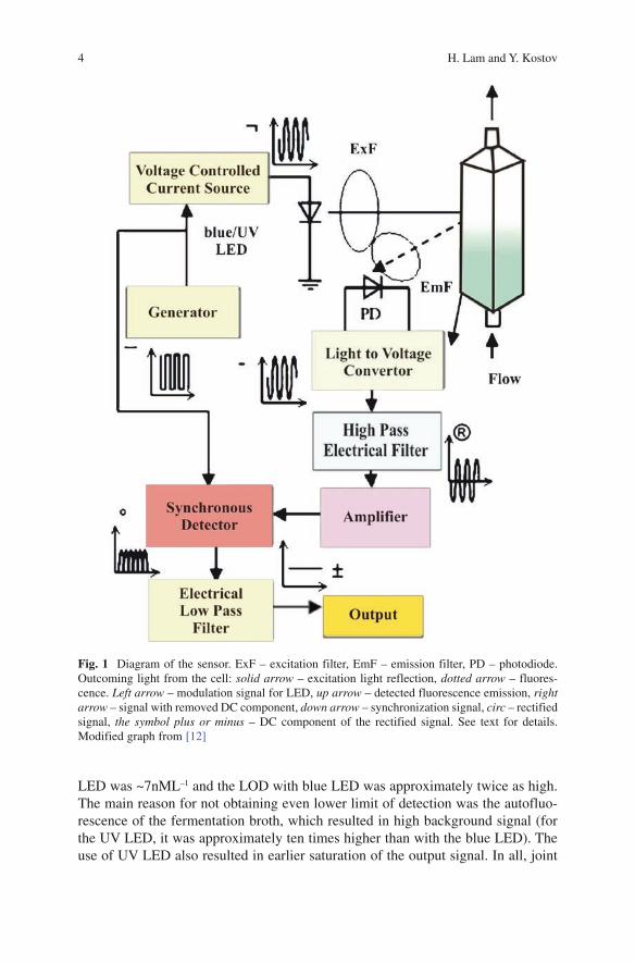
The optoelectronics sensor was designed around a standard 1-cm quartz flow-through cuvette. The cuvette is the only sterilizable part of the sensor. The fermenta-tion broth is pumped aseptically through the cuvette. Front-face illumination and detection geometry was chosen (Fig. 1). The cuvette holder was designed to provide a rigid optical path with constant wavelength. Two excitation LEDs were tested: high-intensity blue LED with peak wavelength at 470nm and brightness 1.6cd and UV emitting LED with peak wavelength at 375nm and power 750 mW. The blue LED was filtered using 470±10-nm band pass filters to remove the “red tail”, while the UV led was not filtered – its emission spectrum was so narrow that no additional filtering was needed. The LEDs were modulated at ~1kHz. The emission was observed through a 514±10-nm filter to pick up the major portion of the green fluo-rescence (GFP emission maximum is at 509nm). After detection and amplification by a photodiode, transimpedance amplifier and several amplification stages (Fig.1) the amplitude of the modulated emission was detected using a home-made lock-in circuit. This amplitude was digitized and recorded by data acquisition system.
The calibration of the sensor is shown in Fig. 2. It exhibits excellent linearity over 3.5 orders of concentrations magnitude with correlation coefficient better than 0.99 for both LEDs). The use of two different LEDs resulted in difference in the sensitivity of the instrument, as expected. Due to the higher power of the UV led and its better spectral match to the major excitation peak the sensitivity of the sensor was approximately four times better. The limit of detection (LOD) with the UV
4 H. Lam and Y. Kostov
LED was ~7nML–1 and the LOD with blue LED was approximately twice as high. The main reason for not obtaining even lower limit of detection was the autofluo-rescence of the fermentation broth, which resulted in high background signal (for the UV LED, it was approximately ten times higher than with the blue LED). The use of UV LED also resulted in earlier saturation of the output signal. In all, joint
Fig. 1 Diagram of the sensor. ExF – excitation filter, EmF – emission filter, PD – photodiode. Outcoming light from the cell: solid arrow – excitation light reflection, dotted arrow – fluores-cence. Left arrow – modulation signal for LED, up arrow – detected fluorescence emission, right arrow – signal with removed DC component, down arrow – synchronization signal, circ – rectified signal, the symbol plus or minus – DC component of the rectified signal. See text for details. Modified graph from [12]

Optical Instrumentation for Bioprocess Monitoring 5
use of these semiconductor light source allows to perform measurements over almost five decade of GFP concentrations.
The reproducibility was quite high; the standard deviation for triple measure-ments was less than 1%. This compares favorably with the fiberoptic version [13] of the sensor, which has a standard deviation of 8%. We attribute the increased repro-ducibility to the fact that a permanent, non-flexible optical path was used (the LED and the photodetector unit were mounted at a distance of ~2mm from the cuvette wall using rigid holder) and the shorter distance between the sample and the detector, which allowed for more light to collected, thus increasing the signal to noise ratio.
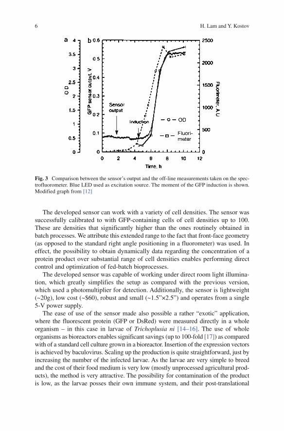
The sensor was validated by comparing it with off-line readings during E. coli fermentation. The strain harbored GFP reporter gene controlled by the arabinose promoter [13]. During the course of the fermentation, samples were collected for off-line measurements of glucose, optical density (OD), and fluorescence intensity. The OD at the end of the processes was 4.6 for the fermentation monitored with the UV LED and 3.5 for the fermentation, monitored with the blue LED. Figure 3 shows the on-line sensor data of the solid-state GFP sensor equipped with blue LED and compared with off-line measurements taken during fermentation. We performed two runs – one monitoring the batch fermentation with the blue, and another with the UV LED. Both the runs showed very high linear correlation (r2=0.989 for UV LED and r2 = 0.998 for blue LED) with the off-line spectrofluorometer measurements.
Fig. 2 Calibration of the GFP sensor with different light sources. Modified graph [12]
6 H. Lam and Y. Kostov
The developed sensor can work with a variety of cell densities. The sensor was successfully calibrated to with GFP-containing cells of cell densities up to 100. These are densities that significantly higher than the ones routinely obtained in batch processes. We attribute this extended range to the fact that front-face geometry (as opposed to the standard right angle positioning in a fluorometer) was used. In effect, the possibility to obtain dynamically data regarding the concentration of a protein product over substantial range of cell densities enables performing direct control and optimization of fed-batch bioprocesses.
The developed sensor was capable of working under direct room light illumina-tion, which greatly simplifies the setup as compared with the previous version, which used a photomultiplier for detection. Additionally, the sensor is lightweight (~20g), low cost (~$60), robust and small (~1.5”×2.5”) and operates from a single 5-V power supply.
The ease of use of the sensor made also possible a rather “exotic” application, where the fluorescent protein (GFP or DsRed) were measured directly in a whole organism – in this case in larvae of Trichoplusia ni [14–16]. The use of whole organisms as bioreactors enables significant savings (up to 100-fold [17]) as compared with of a standard cell culture grown in a bioreactor. Insertion of the expression vectors is achieved by baculovirus. Scaling up the production is quite straightforward, just by increasing the number of the infected larvae. As the larvae are very simple to breed and the cost of their food medium is very low (mostly unprocessed agricultural prod-ucts), the method is very attractive. The possibility for contamination of the product is low, as the larvae posses their own immune system, and their post-translational
Fig. 3 Comparison between the sensor’s output and the off-line measurements taken on the spec-trofluorometer. Blue LED used as excitation source. The moment of the GFP induction is shown. Modified graph from [12]
Optical Instrumentation for Bioprocess Monitoring 7
machinery is significantly better in comparison with bacteria and yeast. However, production of recombinant proteins in this way is not straightforward – endogenous proteases eventually degrade them and lower the yield. Additionally, it is difficult and technically challenging to withdraw samples from the larvae to evaluate the concen-tration of the product. An external sensor that can read the fluorescence intensity of a protein tag can significantly alleviate these problems. The production of such tagged protein is also advantageous from the point of view of the fact that the fused protein interferes with the operation of the proteases, which results in substantial increase of the protein production (>100-fold [17)].
The non-invasive probe used for this application was essentially the same, except that it was using LED (green with peak emission at 525nm and intensity 12cd) as well as different set of filters (525 ± 35nm for excitation and 590 ± 20nm for emission) in order to match the spectral properties of DsRed. Additionally, colored glass filter (OG570) in front of the photodetector was used in order to compensate to some extent for the directional sensitivity of the interference filter. The sensor was assembled in a black box which was relatively easy to handle manu-ally (Fig. 1) or automatically using a robotic positioner.
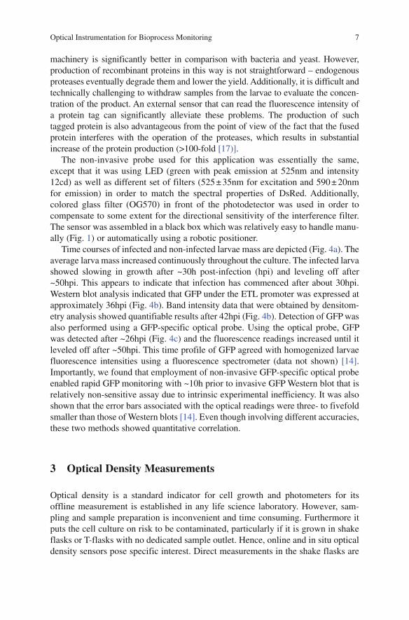
Time courses of infected and non-infected larvae mass are depicted (Fig. 4a). The average larva mass increased continuously throughout the culture. The infected larva showed slowing in growth after ~30h post-infection (hpi) and leveling off after ~50hpi. This appears to indicate that infection has commenced after about 30hpi. Western blot analysis indicated that GFP under the ETL promoter was expressed at approximately 36hpi (Fig. 4b). Band intensity data that were obtained by densitom-etry analysis showed quantifiable results after 42hpi (Fig. 4b). Detection of GFP was also performed using a GFP-specific optical probe. Using the optical probe, GFP was detected after ~26hpi (Fig. 4c) and the fluorescence readings increased until it leveled off after ~50hpi. This time profile of GFP agreed with homogenized larvae fluorescence intensities using a fluorescence spectrometer (data not shown) [14]. Importantly, we found that employment of non-invasive GFP-specific optical probe enabled rapid GFP monitoring with ~10h prior to invasive GFP Western blot that is relatively non-sensitive assay due to intrinsic experimental inefficiency. It was also shown that the error bars associated with the optical readings were three- to fivefold smaller than those of Western blots [14]. Even though involving different accuracies, these two methods showed quantitative correlation.
3 Optical Density Measurements
Optical density is a standard indicator for cell growth and photometers for its offline measurement is established in any life science laboratory. However, sam-pling and sample preparation is inconvenient and time consuming. Furthermore it puts the cell culture on risk to be contaminated, particularly if it is grown in shake flasks or T-flasks with no dedicated sample outlet. Hence, online and in situ optical density sensors pose specific interest. Direct measurements in the shake flasks are
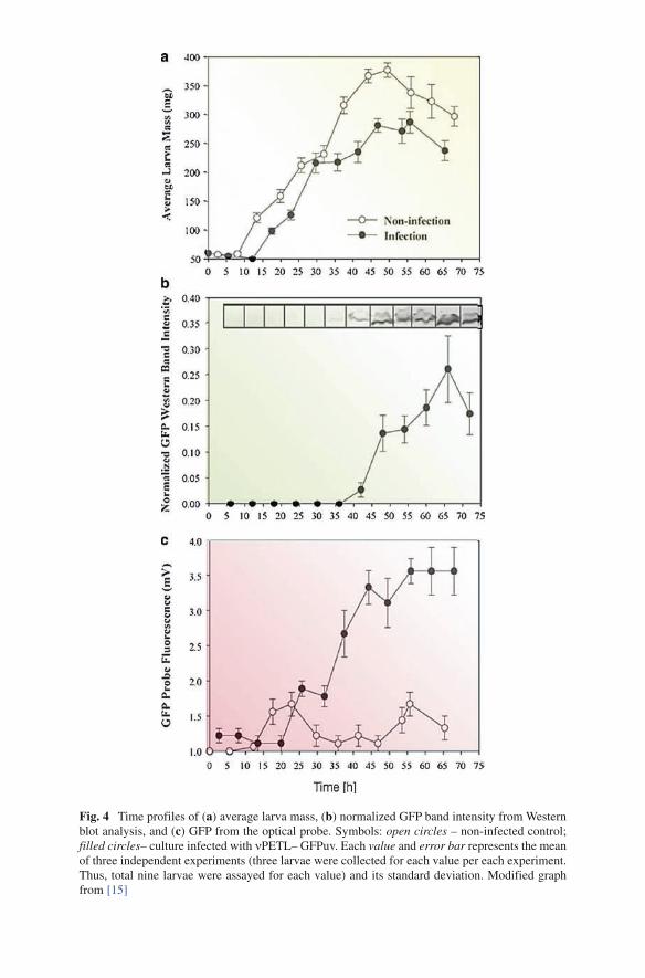
Fig. 4 Time profiles of (a) average larva mass, (b) normalized GFP band intensity from Western blot analysis, and (c) GFP from the optical probe. Symbols: open circles – non-infected control; filled circles– culture infected with nPETL– GFPuv. Each value and error bar represents the mean of three independent experiments (three larvae were collected for each value per each experiment. Thus, total nine larvae were assayed for each value) and its standard deviation. Modified graph from [15]
Optical Instrumentation for Bioprocess Monitoring 9
LED PDLED PD LED PD
Opticalwaveguide
Opticalwaveguide
J-Type Wave Guide Wedge-Type Wave Guide
Fig. 5 Optical configurations for the in situ OD measurement. In the J-type configuration an optical fiber is employed to guide the light in the desired direction, while a prism is used in the wedge-type
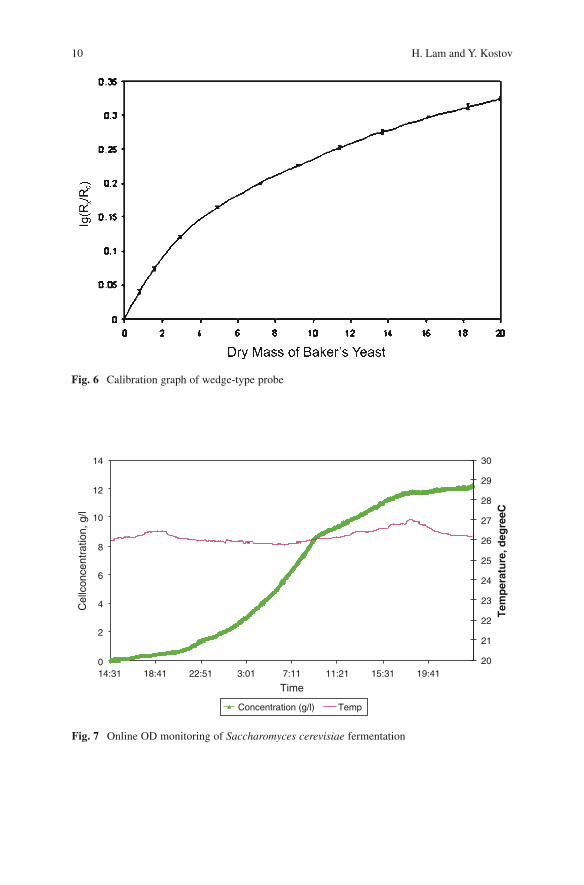
difficult due to the shape of the vessel and the agitation method. Typically, the liquid volume is low, and it is swirled around. This results in periodical increase and decrease of the liquid height (in some cases the liquid layer may get down to 1mm or less). One possible solution (Reference C) is to make use of a special in-flask optical waveguide which ensures that the gap which determines the light path is always filled up with fermentation medium (Fig. 5a,b). Two possible configura-tions were reviewed: J type, which is a regular fiber wave guide, folded in a J shape, and wedge type, which employs two symmetrical wedges. It was found that the J type is less reliable as a path forming device, as the stem changes the hydrodynamic conditions in the flask and generally acts as a baffle. The wedge-type performed the best (visual interpretation), not disturbing the flow.
Calibration curve of the wedge light guide is shown in Fig. 6. The calibration was performed using bakers’ yeast. The curve is quite nonlinear, leveling at around 20gL−1. However, the error of the measurement is remarkably small due to the employed lock-in detection. At high optical densities, the sensitivity is significantly smaller, which a typical feature of the single beam optical density readers. It is well known that a better sensitivity can be achieved using four beam configuration; however, adding more waveguides may obscure the detection gap between the guides from the liquid flow and result in the formation of a stagnant zone.
The sensor was successfully used for monitoring a Saccharomyces cerevisiae fermentation [18] (Fig. 7). The final cell density was also verified by determining the dry cell weight. The sensor operated in the required range and showed the typical growth curve of the yeast. The simplicity of the setup allows the sensor to be used for any kind of shake-flask cultivations; however, individual calibration for different cells may be required.
10 H. Lam and Y. Kostov
0
2
4
6
8
10
12
14
14:31 18:41 22:51 3:01 7:11 11:21 15:31 19:41
Time
Cel
lcon
cent
ratio
n, g
/l
20
21
22
23
24
25
26
27
28
29
30
Tem
per
atu
re, d
egre
eC
Concentration (g/l) Temp
Fig. 7 Online OD monitoring of Saccharomyces cerevisiae fermentation
Fig. 6 Calibration graph of wedge-type probe

Optical Instrumentation for Bioprocess Monitoring 11
4 Ethanol Measurements
Ethanol production is of great importance in clinical, industrial, and biochemical areas as well as in the beverage industry. It is utilized as a solvent in the production of perfumes, paints, lacquers, and explosives. Presently, there is interest in the use of ethanol as a fuel, fuel additive, or a hydrogen source in fuel cells. Ethanol may be produced by the fermentation of fruit, corn, or wheat, or synthetically derived from acetaldehyde or ethylene. With numerous industries that utilize or produce ethanol, reliable methods are needed for its measurement.
There are many analytical methods for determination of ethanol and other alcohols. Broadly, they can be divided into three major categories: chromatographic, enzymatic, and optical. The chromatographic method is the most accurate and sensitive [19, 20] with a lower limit of ethanol detection on the order of 0.005vol.% [21]. Drawbacks of this method include high cost, necessity for sample pretreatment and long operation times. Somewhat less precise but more rapid measurements are achieved by the use of enzymes. Determination of ethanol concentration is based on the use of either of two enzymes – alcohol oxidase or alcohol dehydrogenase. O
2 consumption or H
2O
2 forma-
tion [22, 23] is monitored and related to the ethanol concentration. The specificity of the enzyme binding sites provides highly selective and accurate sensors. However, these enzymes are prone to rapid denaturing, especially when exposed to high tempe-rature, pressure, or pH extremes. Enzyme immobilization in a matrix [24, 25] can enhance somewhat the stability to afford continuous monitoring.
Recently, optical-based sensors received significant attention. They are low-cost and easily manufacturable; they can be readily miniaturized and are intended for use in real-time, in situ monitoring. Lifetime-based [26] and fluorescence-based [27–30] alcohol sensors have been introduced utilizing various alcohol-sensitive dyes. Although extremely promising, these sensors suffer from dye leaching, cross-sensitivity to pH, and low specificity. They also lack high temperature stability due to the presence of plasticizers and are subject to interference due to autofluorescence.
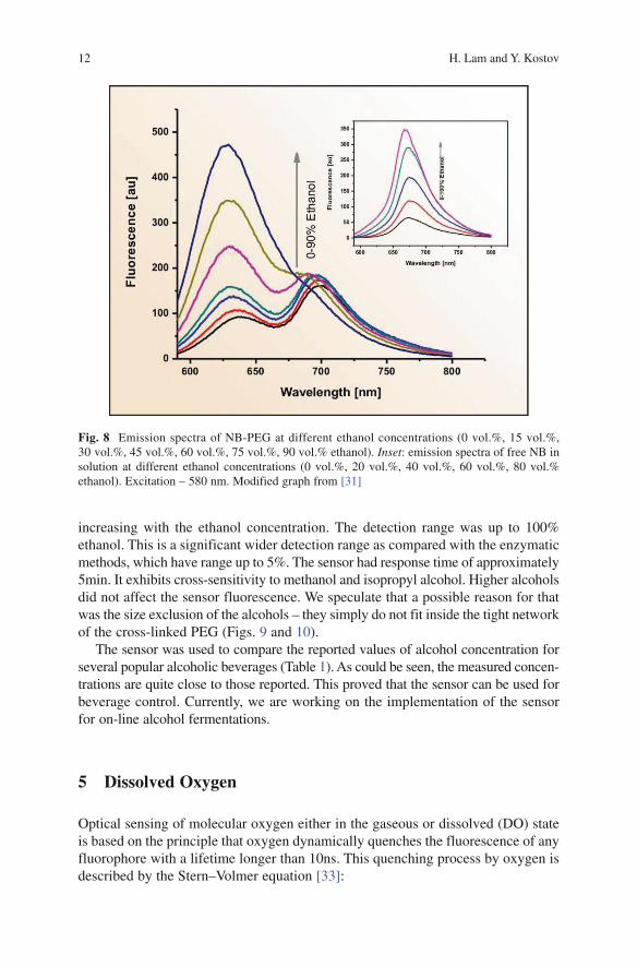
Our group has pioneered the development of plasticizer-free, autoclavable ethanol sensors based on solvatochromic dye immobilized in hydrogel. Nile blue was used due to its NIR emission; this allowed avoiding possible autofluorescence from the sample. The sensor membranes were prepared [31, 32] by Chandrasekharan et al. by incorporating Nile blue methacrylate in polyethyleneglycol diacrylate hydrogel. The resulting hydrogel (NB-PEG) is shaped as film with thickness of ~500 mm. This film exhibits both absorption and fluorescent changes upon contact with ethanol. Here we will discuss only the fluorescence changes.
In the absence of ethanol, the film exhibits fluorescence similar to the one from the free NB. Upon contact with ethanol, the peak at 700nm gradually decreases with the increase of the ethanol concentration; additionally, a new peak develops at 630nm. We assume that this is a result of solvatochromic behaviour of the dye – it is well known that Nile blue exhibits positive solvatochromism. As a result, the emission ratio at the two wavelengths can be used to measure ethanol concentrations (Fig. 8). The threshold of detection was ~1% ethanol, with the sensitivity gradually
12 H. Lam and Y. Kostov
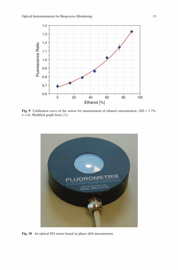
increasing with the ethanol concentration. The detection range was up to 100% ethanol. This is a significant wider detection range as compared with the enzymatic methods, which have range up to 5%. The sensor had response time of approximately 5min. It exhibits cross-sensitivity to methanol and isopropyl alcohol. Higher alcohols did not affect the sensor fluorescence. We speculate that a possible reason for that was the size exclusion of the alcohols – they simply do not fit inside the tight network of the cross-linked PEG (Figs. 9 and 10).
The sensor was used to compare the reported values of alcohol concentration for several popular alcoholic beverages (Table 1). As could be seen, the measured concen-trations are quite close to those reported. This proved that the sensor can be used for beverage control. Currently, we are working on the implementation of the sensor for on-line alcohol fermentations.
5 Dissolved Oxygen
Optical sensing of molecular oxygen either in the gaseous or dissolved (DO) state is based on the principle that oxygen dynamically quenches the fluorescence of any fluorophore with a lifetime longer than 10ns. This quenching process by oxygen is described by the Stern–Volmer equation [33]:
Fig. 8 Emission spectra of NB-PEG at different ethanol concentrations (0 vol.%, 15 vol.%, 30 vol.%, 45 vol.%, 60 vol.%, 75 vol.%, 90 vol.% ethanol). Inset: emission spectra of free NB in solution at different ethanol concentrations (0 vol.%, 20 vol.%, 40 vol.%, 60 vol.%, 80 vol.% ethanol). Excitation – 580 nm. Modified graph from [31]
Optical Instrumentation for Bioprocess Monitoring 13
0 20 40 60 80 1000.6
0.7
0.8
0.9
1.0
1.1
1.2
1.3
1.4
Flu
ores
cenc
e R
atio
Ethanol [%]
Fig. 9 Calibration curve of the sensor for measurement of ethanol concentration. (SD = 1.7%, n = 6). Modified graph from [31]
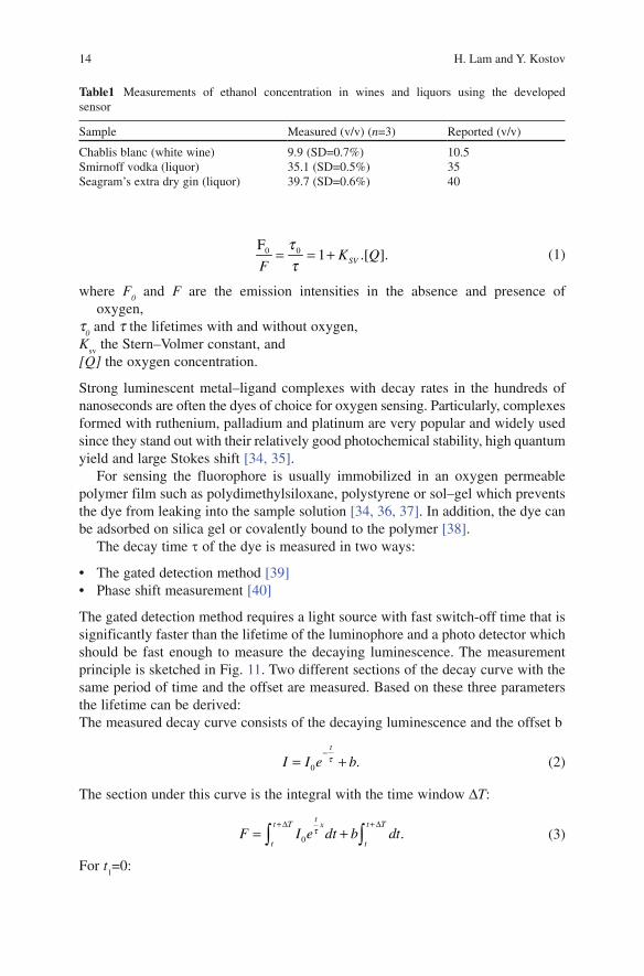
Fig. 10 An optical DO sensor based on phase shift measurement
14 H. Lam and Y. Kostov
0 0 1 .[ ].SVK QF
tt
= = +F
(1)
where F0 and F are the emission intensities in the absence and presence of
oxygen,t
0 and t the lifetimes with and without oxygen,
Ksv
the Stern–Volmer constant, and[Q] the oxygen concentration.
Strong luminescent metal–ligand complexes with decay rates in the hundreds of nanoseconds are often the dyes of choice for oxygen sensing. Particularly, complexes formed with ruthenium, palladium and platinum are very popular and widely used since they stand out with their relatively good photochemical stability, high quantum yield and large Stokes shift [34, 35].
For sensing the fluorophore is usually immobilized in an oxygen permeable polymer film such as polydimethylsiloxane, polystyrene or sol–gel which prevents the dye from leaking into the sample solution [34, 36, 37]. In addition, the dye can be adsorbed on silica gel or covalently bound to the polymer [38].
The decay time t of the dye is measured in two ways:
• The gated detection method [39]• Phase shift measurement [40]
The gated detection method requires a light source with fast switch-off time that is significantly faster than the lifetime of the luminophore and a photo detector which should be fast enough to measure the decaying luminescence. The measurement principle is sketched in Fig. 11. Two different sections of the decay curve with the same period of time and the offset are measured. Based on these three parameters the lifetime can be derived:The measured decay curve consists of the decaying luminescence and the offset b
0
t
I I e bt .−
= + (2)
The section under this curve is the integral with the time window ∆T:
0
tt T t Tx
t tF I e dt b dtt .
+ ∆ + ∆= +∫ ∫ (3)
For t1=0:
Table1 Measurements of ethanol concentration in wines and liquors using the developed sensor
Sample Measured (v/v) (n=3) Reported (v/v)
Chablis blanc (white wine) 9.9 (SD=0.7%) 10.5Smirnoff vodka (liquor) 35.1 (SD=0.5%) 35Seagram’s extra dry gin (liquor) 39.7 (SD=0.6%) 40

Optical Instrumentation for Bioprocess Monitoring 15
∆t∆t
t1
Lu
min
es
ce
nc
e
Time
t2
∆t Offset B
F1
F2
Fig. 11 The lifetime of a luminophore can be measuring the sections F1, F2 and the offset B of a decay curve
1 0 0,
tT
F I e dt Bt∆
= +∫ (4)
2 0
z T
x
tt
tF I e dt Bt .+∆ −
= +∫ (5)
The offset is measured at tz when the luminescence has already decayed:
+ ∆
= ∫ z
z
t T
tB bdt . (6)
After rearranging (4) and (5) the lifetime t is expressed by
= − −
2
2
1
ln
t
F B
F B
t . (7)
The main advantage of this method is that the actual measurement is carried out when the excitation light is switched off. This means the offset is relatively low and no excitation filter is necessary at all. However, as already mentioned, fast optoelectronic components are required for signal acquisition. The photodetector can be a fast photo-multiplier or photodiode. LEDs have become popular as the excitation light source due to its small size, energy efficiency, electronically switchable and low price. Up to date LEDs from UV to infrared emission are commercially available. Basically, the optoelectronics can be set up as described in Fig. 12. At the start of the sensing cycle the light source sends a light pulse to the oxygen sensitive fluorophore (Table 2). The width and timing of the pulse is determined by the microcontroller with the assistance
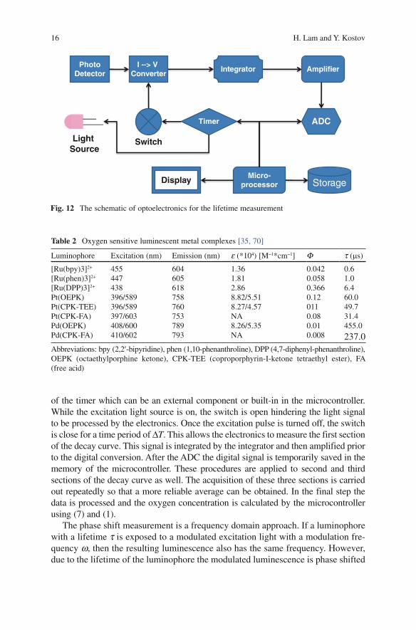
16 H. Lam and Y. Kostov
Table 2 Oxygen sensitive luminescent metal complexes [35, 70]
Luminophore Excitation (nm) Emission (nm) e (*104) [M−1*cm−1] F t (ms)
[Ru(bpy)3]2+ 455 604 1.36 0.042 0.6[Ru(phen)3]2+ 447 605 1.81 0.058 1.0[Ru(DPP)3]2+ 438 618 2.86 0.366 6.4Pt(OEPK) 396/589 758 8.82/5.51 0.12 60.0Pt(CPK-TEE) 396/589 760 8.27/4.57 011 49.7Pt(CPK-FA) 397/603 753 NA 0.08 31.4Pd(OEPK) 408/600 789 8.26/5.35 0.01 455.0Pd(CPK-FA) 410/602 793 NA 0.008 237.0Abbreviations: bpy (2,2¢-bipyridine), phen (1,10-phenanthroline), DPP (4,7-diphenyl-phenanthroline), OEPK (octaethylporphine ketone), CPK-TEE (coproporphyrin-I-ketone tetraethyl ester), FA (free acid)
of the timer which can be an external component or built-in in the microcontroller. While the excitation light source is on, the switch is open hindering the light signal to be processed by the electronics. Once the excitation pulse is turned off, the switch is close for a time period of ∆T. This allows the electronics to measure the first section of the decay curve. This signal is integrated by the integrator and then amplified prior to the digital conversion. After the ADC the digital signal is temporarily saved in the memory of the microcontroller. These procedures are applied to second and third sections of the decay curve as well. The acquisition of these three sections is carried out repeatedly so that a more reliable average can be obtained. In the final step the data is processed and the oxygen concentration is calculated by the microcontroller using (7) and (1).
The phase shift measurement is a frequency domain approach. If a luminophore with a lifetime t is exposed to a modulated excitation light with a modulation fre-quency w, then the resulting luminescence also has the same frequency. However, due to the lifetime of the luminophore the modulated luminescence is phase shifted
PhotoDetector
I --> V Converter
Timer
Amplifier
ADC
Micro-processor
SwitchLight Source
Integrator
Display Storage
Fig. 12 The schematic of optoelectronics for the lifetime measurement

Optical Instrumentation for Bioprocess Monitoring 17
by the angle j (Fig. 13). Intensity-modulated light at a frequency w is generated from an excitation source (an LED in this example). The phase shift j of the result-ing emission is related to the decay time t by the following equation:
=tan( )f
tw
(8)
Hence, the dissolved oxygen concentration [Q]=(DO) can be deduced from (8) and (1). The phase measurement is measured by the lock-in technique. This method requires a frequency reference and the lock-in amplifier detects the response from the measurement at the reference frequency. Supposing the reference signal R has a frequency w and the amplitude I
R:
= sin( ).RR I tw (9)
This signal is used to modulate the excitation light source and serves as the refer-ence for the luminescence signal. The luminescence L arising from the excitation has the same modulation frequency, but it is phase-shifted by an angle of F:
= +sin( ).LL I tw f (10)
The multiplication of the reference and the luminescence signal results in
= + +1
1 1cos( ) sin(2 ).
2 2p R L R LI I I I I tf w f (11)
The first term is a frequency independent value while the second is at a frequency 2w. Hence by passing the signal through a low pass filter the second term is eliminated:
ExcitationEmission
Lig
ht
Inte
nsi
ty
Time
?
IR
IL
Fig. 13 Principle of phase shift measurement. Due to the lifetime of the luminophore the emission curve is phase shifted by angle of j. The modulation frequency remains unchanged
18 H. Lam and Y. Kostov
1
cos( ).2LPI R LI I I f= (12)
If the reference signal, which is 90° out of phase, is used for the multiplication, the resulting product is
2
1 1cos sin 2 .
2 2 2 2p R L R LI I I I I t +p p
f w f = − + − (13)
Then, after low pass filtering it is
LP2
1sin( ).
2 R LI I I f= (14)
By dividing (12) by (14) the following term is obtained and the lifetime can be calculated:
LP1
LP2
tan( ).I
If= (15)
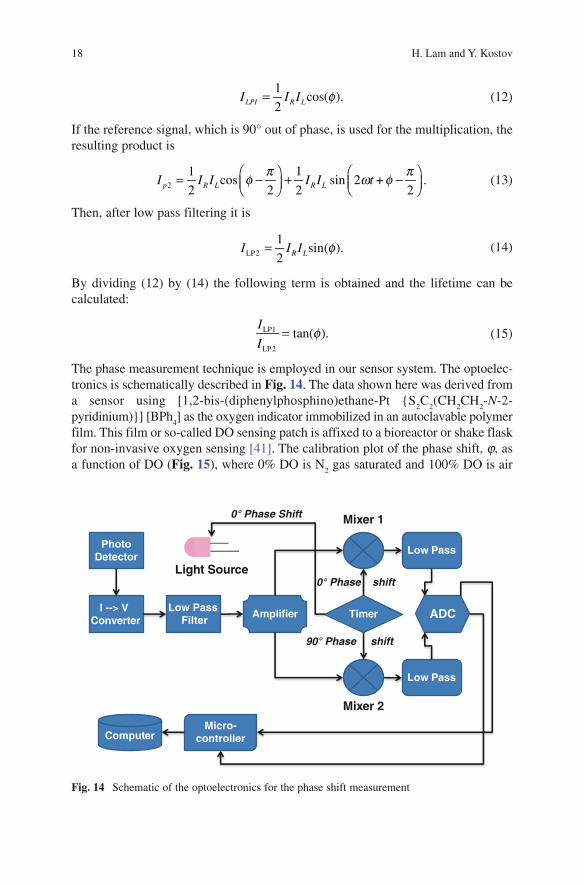
The phase measurement technique is employed in our sensor system. The optoelec-tronics is schematically described in Fig. 14. The data shown here was derived from a sensor using [1,2-bis-(diphenylphosphino)ethane-Pt {S
2C
2(CH
2CH
2-N-2-
pyridinium)}] [BPh4] as the oxygen indicator immobilized in an autoclavable polymer
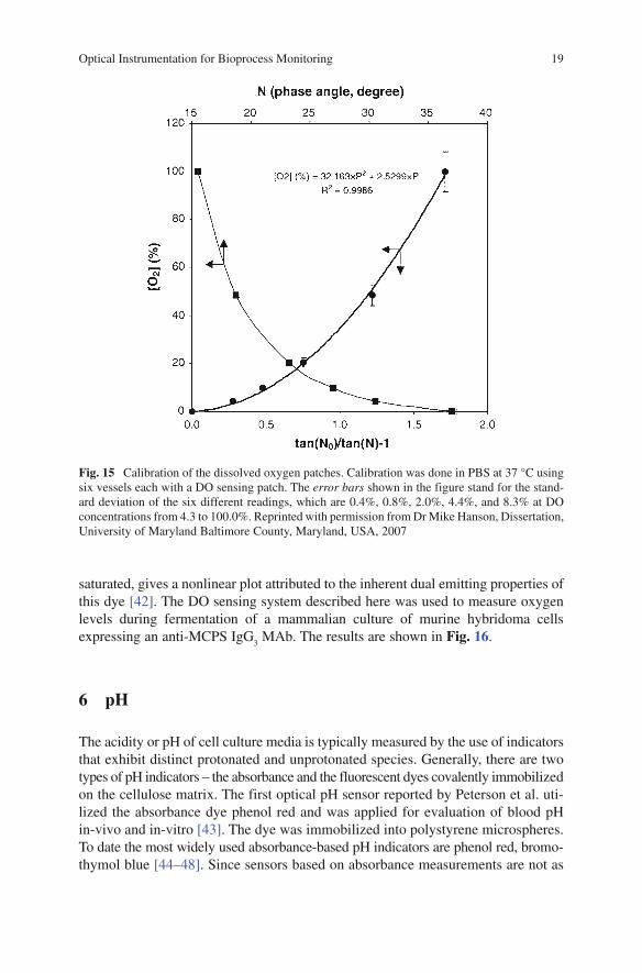
film. This film or so-called DO sensing patch is affixed to a bioreactor or shake flask for non-invasive oxygen sensing [41]. The calibration plot of the phase shift, j, as a function of DO (Fig. 15), where 0% DO is N
2 gas saturated and 100% DO is air
PhotoDetector
I --> V Converter
TimerLow Pass
Filter
Low Pass
ADC
Micro-controller
Mixer 1
Light Source
Amplifier
Computer
90° Phase shift
0° Phase shift
Low Pass
Mixer 2
0° Phase Shift
Fig. 14 Schematic of the optoelectronics for the phase shift measurement
Optical Instrumentation for Bioprocess Monitoring 19
Fig. 15 Calibration of the dissolved oxygen patches. Calibration was done in PBS at 37 °C using six vessels each with a DO sensing patch. The error bars shown in the figure stand for the stand-ard deviation of the six different readings, which are 0.4%, 0.8%, 2.0%, 4.4%, and 8.3% at DO concentrations from 4.3 to 100.0%. Reprinted with permission from Dr Mike Hanson, Dissertation, University of Maryland Baltimore County, Maryland, USA, 2007
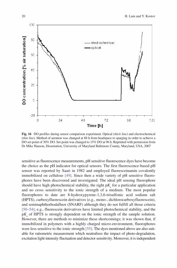
saturated, gives a nonlinear plot attributed to the inherent dual emitting properties of this dye [42]. The DO sensing system described here was used to measure oxygen levels during fermentation of a mammalian culture of murine hybridoma cells expressing an anti-MCPS IgG
3 MAb. The results are shown in Fig. 16.
6 pH
The acidity or pH of cell culture media is typically measured by the use of indicators that exhibit distinct protonated and unprotonated species. Generally, there are two types of pH indicators – the absorbance and the fluorescent dyes covalently immobilized on the cellulose matrix. The first optical pH sensor reported by Peterson et al. uti-lized the absorbance dye phenol red and was applied for evaluation of blood pH in-vivo and in-vitro [43]. The dye was immobilized into polystyrene microspheres. To date the most widely used absorbance-based pH indicators are phenol red, bromo-thymol blue [44–48]. Since sensors based on absorbance measurements are not as
20 H. Lam and Y. Kostov
sensitive as fluorescence measurements, pH sensitive fluorescence dyes have become the choice as the pH indicator for optical sensors. The first fluorescence-based pH sensor was reported by Saari in 1982 and employed fluoresceinamin covalently immobilized on cellulose [49]. Since then a wide variety of pH sensitive fluoro-phores have been discovered and investigated. The ideal pH sensing fluorophore should have high photochemical stability, the right pK
a for a particular application
and no cross sensitivity to the ionic strength of a medium. The most popular fluorophores to date are 8-hydroxypyrene-1,3,6-trisulfonic acid sodium salt (HPTS), carboxyfluorescein derivatives (e.g., mono-, dichlorocarboxyfluorescein), and seminaphthorhodafluor (SNARF) although they do not fulfill all those criteria [50–54]; e.g., fluorescein derivatives have limited photochemical stability, and the pK
a of HPTS is strongly dependent on the ionic strength of the sample solution.
However, there are methods to minimize these shortcomings; it was shown that, if immobilized in polymers with a highly charged micro-environment, fluorophores were less sensitive to the ionic strength [55]. The dyes mentioned above are also suit-able for ratiometric measurement which neutralizes the impact of photo-degradation, excitation light intensity fluctuation and detector sensitivity. Moreover, it is independent
Fig. 16 DO profiles during sensor comparison experiment. Optical (thick line) and electrochemical (thin line). Method of aeration was changed at 88 h from headspace to sparging in order to achieve a DO set-point of 30% DO. Set-point was changed to 15% DO at 96 h. Reprinted with permission from Dr Mike Hanson, Dissertation, University of Maryland Baltimore County, Maryland, USA, 2007

Optical Instrumentation for Bioprocess Monitoring 21
of the concentration of the fluorescence dyes. In principle there are two types of these fluorescent indicators. Dual excitation indicators are similar to the absorption-based indicators in that their basic and acidic forms possess different absorption maxima and extinction coefficients. The emission maxima, however, may be unaffected by pH, as the emission originates from the same transition state after internal conversion, but the quantum yield (i.e., emission intensity) is dependent on excitation wavelength. Thus, one can measure the emission intensities at two excitation wavelengths, and the ratio of the emission intensities becomes a function of pH. Examples of this type of fluorescent pH indicator include hydroxypyrene trisulfonic acid (HPTS), carboxy-diclorofluorescein (CDCF), carboxynaphtofluorescein (CNF), etc.
A second type of pH sensor is the emission-ratiometric indicator. In this case, not only the excitation maxima but also the emission spectra are different for the acid and base forms. One can then relate the ratio of intensities at two emission wave-lengths to pH. Examples of these are the SNAFLs and SNARFs (Molecular Probes, Inc., Eugene, Oregon). In both types of pH sensor, the relationship between the observed and the proton concentration is given by the following equation [56]:
1( )
[)
] . .(
max A Aa
min HA HA
R RH k
R R
ee
−+ Φ−=
− Φ (16)
with Rmin
, Rmax
the ratios for the acid (HA) and conjugate base (A−), respectively,e the extinction coefficient,F the quantum yield of each species evaluated at l
2,
and ka equilibrium dissociation constant.
A good example of an optical pH sensor that has been successfully used in bioproc-ess monitoring is HPTS and its derivatives. This dye exhibits two excitation wave-lengths, one UV (l
1=405nm) and one blue (l
2=457nm), that correspond to the acid
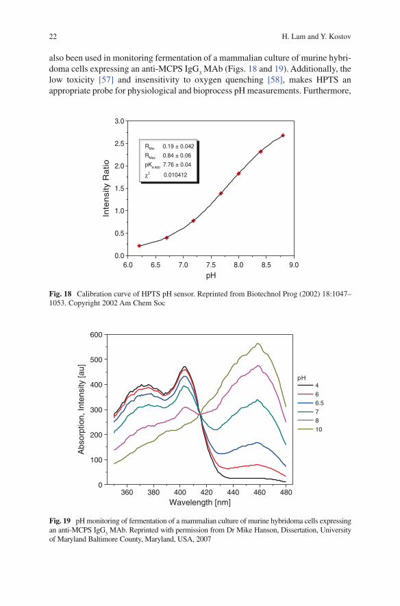
and its conjugate base. The ratio of emission intensities at 530nm, R, for these two wavelengths is related to the proton concentration as shown in Fig. 17. With a pK
a
of 7.3, HPTS is suitable for ratiometric detection in the physiological range. It has
Fig. 17 Excitation spectra of HPTS (lemission
= 515 nm) immobilized in PEG-Dowex
22 H. Lam and Y. Kostov
6.0 6.5 7.0 7.5 8.0 8.5 9.00.0
0.5
1.0
1.5
2.0
2.5
3.0
Inte
nsi
ty R
atio
pH
RMin 0.19 ± 0.042
RMax 0.84 ± 0.06
pKa,app 7.76 ± 0.04
χ2 0.010412
Fig. 18 Calibration curve of HPTS pH sensor. Reprinted from Biotechnol Prog (2002) 18:1047–1053. Copyright 2002 Am Chem Soc
360 380 400 420 440 460 4800
100
200
300
400
500
600
pH466.57810
Abs
orpt
ion,
Inte
nsity
[au]
Wavelength [nm]
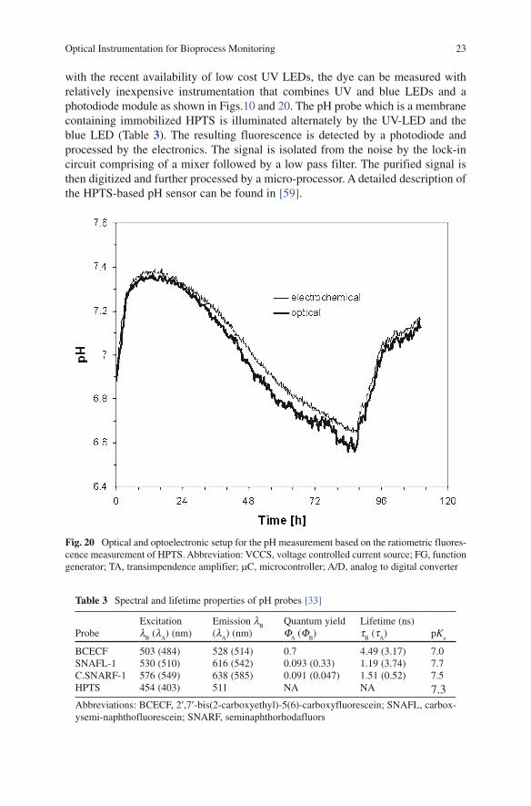
Fig. 19 pH monitoring of fermentation of a mammalian culture of murine hybridoma cells expressing an anti-MCPS IgG
3 MAb. Reprinted with permission from Dr Mike Hanson, Dissertation, University
of Maryland Baltimore County, Maryland, USA, 2007
also been used in monitoring fermentation of a mammalian culture of murine hybri-doma cells expressing an anti-MCPS IgG
3 MAb (Figs. 18 and 19). Additionally, the
low toxicity [57] and insensitivity to oxygen quenching [58], makes HPTS an appropriate probe for physiological and bioprocess pH measurements. Furthermore,
Optical Instrumentation for Bioprocess Monitoring 23
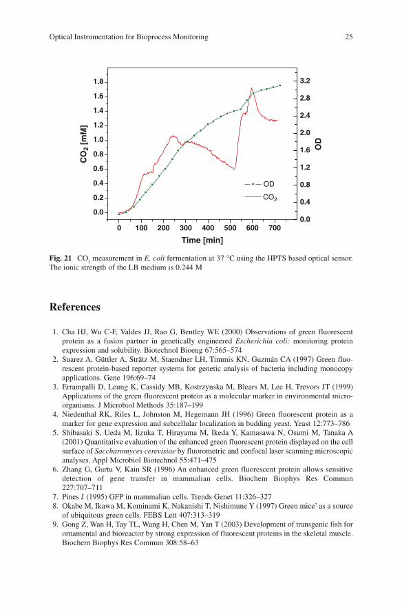
Table 3 Spectral and lifetime properties of pH probes [33]
ProbeExcitation l
B (l
A) (nm)
Emission lB
(lA) (nm)
Quantum yield F
A (F
B)
Lifetime (ns) t
B (t
A) pK
a
BCECF 503 (484) 528 (514) 0.7 4.49 (3.17) 7.0SNAFL-1 530 (510) 616 (542) 0.093 (0.33) 1.19 (3.74) 7.7C.SNARF-1 576 (549) 638 (585) 0.091 (0.047) 1.51 (0.52) 7.5HPTS 454 (403) 511 NA NA 7.3Abbreviations: BCECF, 2¢,7¢-bis(2-carboxyethyl)-5(6)-carboxyfluorescein; SNAFL, carbox-ysemi-naphthofluorescein; SNARF, seminaphthorhodafluors
Fig. 20 Optical and optoelectronic setup for the pH measurement based on the ratiometric fluores-cence measurement of HPTS. Abbreviation: VCCS, voltage controlled current source; FG, function generator; TA, transimpendence amplifier; mC, microcontroller; A/D, analog to digital converter
with the recent availability of low cost UV LEDs, the dye can be measured with relatively inexpensive instrumentation that combines UV and blue LEDs and a photodiode module as shown in Figs.10 and 20. The pH probe which is a membrane containing immobilized HPTS is illuminated alternately by the UV-LED and the blue LED (Table 3). The resulting fluorescence is detected by a photodiode and processed by the electronics. The signal is isolated from the noise by the lock-in circuit comprising of a mixer followed by a low pass filter. The purified signal is then digitized and further processed by a micro-processor. A detailed description of the HPTS-based pH sensor can be found in [59].

24 H. Lam and Y. Kostov
7 Carbon Dioxide
The earlier design of optical CO2 sensors copies the concept of the Severinghaus
electrode [60], in which a pH-sensitive electrode or indicator is in contact with a thin layer of bicarbonate solution encapsulated by a thin, gas-permeable mem-brane. As CO
2 diffuses into this membrane it dissolves into the bicarbonate solu-
tion, resulting in a change in pH which is measured by a pH sensitive optical probe. In practice, the CO
2 optical sensor with this design is not very favorable for bio-
process applications because of several drawbacks that include interferences by acidic and basic gases, slow response time and negative effects of osmotic pressure [61]. In a new design first reported by Mills et al. [62–65], these shortcomings are eliminated by the replacement of the bicarbonate buffer with a phase transfer agent, namely a quaternary ammonium hydroxide (QMH) and the gas-permeable mem-brane with a hydrophobic polymer. This phase transfer agent serves several pur-poses: (1) it aids in dissolving the indicator dye in the hydrophobic polymer by forming an ion pair with the indicator dye anion [66, 67]; (2) due to its hygroscopic character it allows for the incorporation of moisture in the polymer, which is needed in the overall acid-base reaction; (3) it provides the basic environment essential for CO
2 sensing.
The sensing mechanism for such a film [68] is summarized by the following equation:
{ } { }2 2 3 2Q A xH O CO Q HCO (x 1)H O HA.+ − + −• + ⇔ • − +
Basically, in the aqueous micro-environment surrounding the ion pair, CO2 forms
with one water molecule H2CO
3 which protonates the pH sensitive fluorophore in
its anion form A− and converts it into its free acid form HA. Simultaneously, HCO3
− replaces A− as the counter ion for Q+. This reversible reaction causes the fluores-cence change that correlates with the CO
2 concentration. The use of HPTS as the
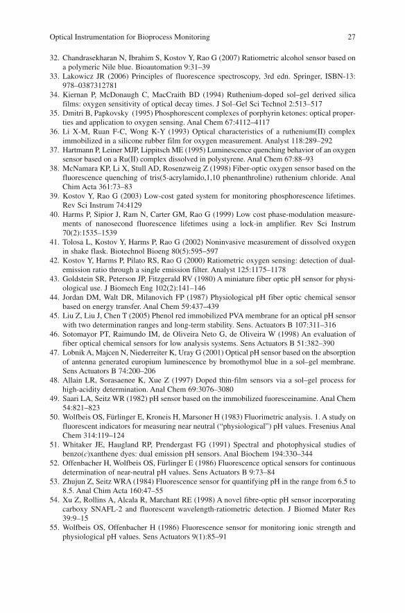
pH indicator for this sensor is convenient because it allows for using the same optics, electronics and software as in the pH sensor described in the previous sec-tion. Sample data obtained from a fermentation experiment using this sensor to monitor CO
2 are shown in Fig. 21. Readers are advised to consult reference [69] for
a more exhaustive account of the fabrication of this CO2 sensor. Another variation
of this approach is reported by Wolfbeis et al. [68]. Instead of using a pH sensitive fluorophore which measures the pH change directly, the pH sensitive absorbance dye thymol blue and ruthenium(II)-4,4-diphenyl-2,2-bipyridyl were employed. The measurement principle is based on the radiationless energy transfer from the ruthe-nium complex (donor) to thymol blue (acceptor). This process occurs since the absorption spectrum of the thymol blue overlaps with the emission spectrum of the ruthenium complex. However, with increasing CO
2 concentration, thymol blue
becomes more protonated, resulting in a decrease of energy transfer. This has an effect not only on the fluorescence intensity but also on the fluorescence lifetime of the ruthenium complex. Thus, the lifetime change serves as the indicator of the CO
2
concentration.
Optical Instrumentation for Bioprocess Monitoring 25
References
1. Cha HJ, Wu C-F, Valdes JJ, Rao G, Bentley WE (2000) Observations of green fluorescent protein as a fusion partner in genetically engineered Escherichia coli: monitoring protein expression and solubility. Biotechnol Bioeng 67:565–574
2. Suarez A, Güttler A, Strätz M, Staendner LH, Timmis KN, Guzmán CA (1997) Green fluo-rescent protein-based reporter systems for genetic analysis of bacteria including monocopy applications. Gene 196:69–74
3. Errampalli D, Leung K, Cassidy MB, Kostrzynska M, Blears M, Lee H, Trevors JT (1999) Applications of the green fluorescent protein as a molecular marker in environmental micro-organisms. J Microbiol Methods 35:187–199
4. Niedenthal RK, Riles L, Johnston M, Hegemann JH (1996) Green fluorescent protein as a marker for gene expression and subcellular localization in budding yeast. Yeast 12:773–786
5. Shibasaki S, Ueda M, Iizuka T, Hirayama M, Ikeda Y, Kamasawa N, Osumi M, Tanaka A (2001) Quantitative evaluation of the enhanced green fluorescent protein displayed on the cell surface of Saccharomyces cerevisiae by fluorometric and confocal laser scanning microscopic analyses. Appl Microbiol Biotechnol 55:471–475
6. Zhang G, Gurtu V, Kain SR (1996) An enhanced green fluorescent protein allows sensitive detection of gene transfer in mammalian cells. Biochem Biophys Res Commun 227:707–711
7. Pines J (1995) GFP in mammalian cells. Trends Genet 11:326–327 8. Okabe M, Ikawa M, Kominami K, Nakanishi T, Nishimune Y (1997) Green mice’ as a source
of ubiquitous green cells. FEBS Lett 407:313–319 9. Gong Z, Wan H, Tay TL, Wang H, Chen M, Yan T (2003) Development of transgenic fish for
ornamental and bioreactor by strong expression of fluorescent proteins in the skeletal muscle. Biochem Biophys Res Commun 308:58–63
0 100 200 300 400 500 600 700
0.0
0.2
0.4
0.6
0.8
1.0
1.2
1.4
1.6
1.8
0.0
0.4
0.8
1.2
1.6
2.0
2.4
2.8
3.2
CO
2 [m
M]
Time [min]
CO2
OD
OD
Fig. 21 CO2 measurement in E. coli fermentation at 37 °C using the HPTS based optical sensor.
The ionic strength of the LB medium is 0.244 M

26 H. Lam and Y. Kostov
10. DeLisa MP, Li J, Rao G, Weigand WA, Bentley WE (1999) Monitoring GFP-operon fusion protein expression during high cell density cultivation of Escherichia coli using an on-line optical sensor. Biotechnol Bioeng 65:54–64
11. Randers-Eichhorn L, Albano CR, Sipior J, Bentley WE, Rao G (1997) On-line green fluorescent protein sensor with LED excitation. Biotechnol Bioeng 55:921–926
12. Kostov Y, Albano CR, Rao G (2000) All solid-state GFP sensor. Biotechnol Bioeng 70:473–477
13. Crameri A, Whitehorn EA, Tate E, Stemmer WPC (1996) Improved green fluorescent protein by molecular evolution using DNA shuffling. Nat Biotechnol 14:315–319
14. Kramer SF, Kostov Y, Rao G, Bentley WE (2003) Ex vivo monitoring of protein production in baculovirus-infected Trichoplusia ni larvae with a GFP-specific optical probe. Biotechnol Bioeng 83:241–247
15. Dalal NG, Cha HJ, Kramer SF, Kostov Y, Rao G, Bentley WE (2006) Rapid non-invasive moni-toring of baculovirus infection for insect larvae using green fluorescent protein reporter under early-to-late promoter and a GFP-specific optical probe. Process Biochem 41(4):947–950
16. Kostov Y, Tolosa L, O’Connell K, Anderson P, Liu Y, van Beek N, Rao G (2003) Monitoring of DsRed protein concentration in frozen insect larvae. Proceedings SPIE, vol 4967, pp 100–107
17. Cha HJ, Dalal NG, Pham MQ, Vakharia VN, Rao G, Bentley WE (1999) Insect larval expres-sion process is optimized by generating fusions with green fluorescent protein. Biotechnol Bioeng 65:316–324
18. Kostov Y, Harms P, Rao G (2002) On-line optical density measurements in shake flasks. 224th ACS National Meeting, Boston MA, August
19. Buttler T, Johansson KAJ, Gorton LGO, Marko-Varga GA (1993) On-line fermentation proc-ess monitoring of carbohydrates and ethanol using tangential flow filtration and column liquid chromatography. Anal Chem 65:2628–2636
20. Johansson K, Jonsson-Petterson G, Gorton L, Marko-Varga G, Csoregi E (1993) A reagentless amperometric biosensor for alcohol detection in column liquid chromatography based on co-immobilized peroxidase and alcohol oxidase in carbon paste. J Biotechnol 31:301–316
21. Zinbo M (1994) Determination of one carbon to three-carbon alcohols and water ingasoline/alcohol blends by liquid chromatography. Anal Chem 56:244–247
22. Azevedo AM, Prazeres DMF, Cabral JMS, Fonseca LP (2005) Ethanol biosensors based on alcohol oxidase. Biosens Bioelectron 21:235–247
23. Boujitita M, Hart JP, Pittson R (2000) Development of a disposable ethanol biosensor based on a chemically modified screen-printed electrode coated with alcohol oxidase for the analysis of beer. Biosens Bioelectron 15:257–263
24. Belghith H, Romette J-L, Thomas D (1987) An enzyme electrode for on-line determination of ethanol and methanol. Biotechnol Bioeng 30:1001–1005
25. Mitsubayashi K, Yokoyama K, Takeuchi T, Karube I (1994) Gas-phase biosensor for ethanol. Anal Chem 66:3297–3302
26. Chang Q, Lakowicz JR, Rao G (1997) Fluorescence lifetime-based sensing of methanol. Analyst 122:173–177
27. Mohr GJ, Lehmann F, Grummt U-W, Spichiger-Keller UE (1997) Fluorescent ligands for optical sensing of alcohols: synthesis and characterization of p-N,N-dialkylamino-trifluoroacetylstilbenes. Anal Chim Acta 344:215–225
28. Mohr GJ, Spichiger-Keller UE (1997) Novel fluorescent sensor membranes for alcohol based on p-N,N-dioctylamino-4¢-trifluoroacetylstilben. Anal Chim Acta 351:189–196
29. Blum P, Mohr GJ, Matern K, Reichert J, Spichiger-Keller UE (2001) Optical alcohol sensor using lipophilic Reichardt’s dyes in polymer membranes. Anal Chim Acta 432:269–275
30. Orellana G, Gomez-Carneros AM, de Dios C, Garcia-Mertinez AA, Moreno-Bondi MC (1995) Reversible fiber-optic fluorescing of lower alcohols. Anal Chem 67:2231–2238
31. Petrova S, Kostov Y, Jeffris K, Rao G (2007) Optical ratiometric sensor for alcohol measure-ments. Anal Lett 40:715–727
Optical Instrumentation for Bioprocess Monitoring 27
32. Chandrasekharan N, Ibrahim S, Kostov Y, Rao G (2007) Ratiometric alcohol sensor based on a polymeric Nile blue. Bioautomation 9:31–39
33. Lakowicz JR (2006) Principles of fluorescence spectroscopy, 3rd edn. Springer, ISBN-13: 978–0387312781
34. Kiernan P, McDonaugh C, MacCraith BD (1994) Ruthenium-doped sol–gel derived silica films: oxygen sensitivity of optical decay times. J Sol–Gel Sci Technol 2:513–517
35. Dmitri B, Papkovsky (1995) Phosphorescent complexes of porphyrin ketones: optical proper-ties and application to oxygen sensing. Anal Chem 67:4112–4117
36. Li X-M, Ruan F-C, Wong K-Y (1993) Optical characteristics of a ruthenium(II) complex immobilized in a silicone rubber film for oxygen measurement. Analyst 118:289–292
37. Hartmann P, Leiner MJP, Lippitsch ME (1995) Luminescence quenching behavior of an oxygen sensor based on a Ru(II) complex dissolved in polystyrene. Anal Chem 67:88–93
38. McNamara KP, Li X, Stull AD, Rosenzweig Z (1998) Fiber-optic oxygen sensor based on the fluorescence quenching of tris(5-acrylamido,1,10 phenanthroline) ruthenium chloride. Anal Chim Acta 361:73–83
39. Kostov Y, Rao G (2003) Low-cost gated system for monitoring phosphorescence lifetimes. Rev Sci Instrum 74:4129
40. Harms P, Sipior J, Ram N, Carter GM, Rao G (1999) Low cost phase-modulation measure-ments of nanosecond fluorescence lifetimes using a lock-in amplifier. Rev Sci Instrum 70(2):1535–1539
41. Tolosa L, Kostov Y, Harms P, Rao G (2002) Noninvasive measurement of dissolved oxygen in shake flask. Biotechnol Bioeng 80(5):595–597
42. Kostov Y, Harms P, Pilato RS, Rao G (2000) Ratiometric oxygen sensing: detection of dual-emission ratio through a single emission filter. Analyst 125:1175–1178
43. Goldstein SR, Peterson JP, Fitzgerald RV (1980) A miniature fiber optic pH sensor for physi-ological use. J Biomech Eng 102(2):141–146
44. Jordan DM, Walt DR, Milanovich FP (1987) Physiological pH fiber optic chemical sensor based on energy transfer. Anal Chem 59:437–439
45. Liu Z, Liu J, Chen T (2005) Phenol red immobilized PVA membrane for an optical pH sensor with two determination ranges and long-term stability. Sens. Actuators B 107:311–316
46. Sotomayor PT, Raimundo IM, de Oliveira Neto G, de Oliveira W (1998) An evaluation of fiber optical chemical sensors for low analysis systems. Sens Actuators B 51:382–390
47. Lobnik A, Majcen N, Niederreiter K, Uray G (2001) Optical pH sensor based on the absorption of antenna generated europium luminescence by bromothymol blue in a sol–gel membrane. Sens Actuators B 74:200–206
48. Allain LR, Sorasaenee K, Xue Z (1997) Doped thin-film sensors via a sol–gel process for high-acidity determination. Anal Chem 69:3076–3080
49. Saari LA, Seitz WR (1982) pH sensor based on the immobilized fuoresceinamine. Anal Chem 54:821–823
50. Wolfbeis OS, Fürlinger E, Kroneis H, Marsoner H (1983) Fluorimetric analysis. 1. A study on fluorescent indicators for measuring near neutral (“physiological”) pH values. Fresenius Anal Chem 314:119–124
51. Whitaker JE, Haugland RP, Prendergast FG (1991) Spectral and photophysical studies of benzo(c)xanthene dyes: dual emission pH sensors. Anal Biochem 194:330–344
52. Offenbacher H, Wolfbeis OS, Fürlinger E (1986) Fluorescence optical sensors for continuous determination of near-neutral pH values. Sens Actuators B 9:73–84
53. Zhujun Z, Seitz WRA (1984) Fluorescence sensor for quantifying pH in the range from 6.5 to 8.5. Anal Chim Acta 160:47–55
54. Xu Z, Rollins A, Alcala R, Marchant RE (1998) A novel fibre-optic pH sensor incorporating carboxy SNAFL-2 and fluorescent wavelength-ratiometric detection. J Biomed Mater Res 39:9–15
55. Wolfbeis OS, Offenbacher H (1986) Fluorescence sensor for monitoring ionic strength and physiological pH values. Sens Actuators 9(1):85–91
28 H. Lam and Y. Kostov
56. Tsien RY (1989) Fluorescent indicators of ion concentrations. Methods Cell Biol 30:127–156
57. Lutty GA (1978) The acute intravenous toxicity of stains, dyes, and other fluorescent substances. Toxicol Pharmacol 44:225–229
58. Zhujun Z, Sitz WRA (1984) Fluorescence sensor for quantifying pH in the range from 6.5 to 8.5. Anal Chim Acta 160:47–55
59. Kermis HR, Kostov Y, Harms P, Rao G (2002) Dual excitation ratiometric fluorescent pH sensor for noninvasive bioprocess monitoring: development and application. Biotechnol Prog 18:1047–1053
60. Severinghaus JW, Bradley AF (1958) Electrodes for blood pO2 and pCO2 determination. J Physiol 13:515–520
61. Weidgans BM (2004) New fluorescent pH-sensor with minimal effects of ionic strength. Dissertation, University of Regensburg, Germany
62. Mills A, Chang Q, McMurray N (1992) Anal Chem 64:138363. Mills A, Chang Q (1993) Analyst 118:83964. Mills A, Chang Q (1994) Sens Actuators B 21:8365. Mills A, Lepre A, Wild L (1997) Sens Actuators B: 383966. Chang Q, Randers-Eichhorn L, Lakowicz JR, Rao G (1998) Steam-sterilizable, fluorescence
lifetime-based sensing film for dissolved CO2. Biotechnol Prog 14(2):326–33167. Sipior J, Randers-Eichhorn L, Lakowicz JR, Carter CM, Rao G (1996) Phase fluorometric
optical carbon dioxide gas sensor for fermentation off-gas monitoring. Biotechnol Prog 12:266–271
68. Neurauter G, Klimant I, Wolfbeis OS (1999) Microsecond lifetime-based optical carbondiox-ide sensor using luminescence resonance energy transfer. Anal Chim Acta 382:6775
69. Ge X, Kostov Y, Rao G (2003) High-stability non-invasive autoclavable naked optical CO2 sensor. Biosensors Bioelectron 18:857–865
70. Hung T Lam (2002) development and applications of fiberoptical chemo and biosensors in biotechnology. Dissertation, University of Hannover, Germany
Plasmon-Controlled Fluorescence Towards High-Sensitivity Optical Sensing
K. Ray, M. H. Chowdhury, J. Zhang, Y. Fu, H. Szmacinski, K. Nowaczyk, and J. R. Lakowicz
K. Ray, M.H. Chowdhury, J. Zhang, Y. Fu, H. Szmainski, K. Nowaczyk, and J.R. Lakowicz (*ü )Center for Fluorescence Spectroscopy, Department of Biochemistry and Molecular Biology, University of Maryland School of Medicine, 725 W Lombard St, Baltimore, MD 21201, USA
Abstract Fluorescence spectroscopy is widely used in chemical and biological research. Until recently most of the fluorescence experiments have been performed in the far-field regime. By far-field we imply at least several wavelengths from the fluorescent probe molecule. In recent years there has been growing interest in the interactions of fluorophores with metallic surfaces or particles. Near-field interac-tions are those occurring within a wavelength distance of an excited fluorophore. The spectral properties of fluorophores can dramatically be altered by near-field interactions with the electron clouds present in metals. These interactions modify the emission in ways not seen in classical fluorescence experiments. Fluorophores in the excited state can create plasmons that radiate into the far-field and fluorophores in the ground state can interact with and be excited by surface plasmons. These recip-rocal interactions suggest that the novel optical absorption and scattering properties of metallic nanostructures can be used to control the decay rates, location, and direction of fluorophore emission. We refer to these phenomena as plasmon-con-trolled fluorescence (PCF). An overview of the recent work on metal—fluorophore interactions is presented. Recent research combining plasmonics and fluorescence suggest that PCF could lead to new classes of experimental procedures, novel probes, bioassays, and devices.
Keywords Fluorescence, Metal-enhanced fluorescence, Plasmon-controlled fluo-rescence, Sensing, Single molecule detection, Surface-plasmon coupled emission
Adv Biochem Engin/Biotechnol (2009) 116: 29–72DOI: 10.1007/10_2008_9© Springer-Verlag Berlin Heidelberg 200Published online: 01 October 2008
9

30 K. Ray et al.
1 Introduction
In recent years there has been growing interest in investigating the interactions of fluorophores with metallic surfaces or particles. Recent research from this laboratory has revealed a number of important effects, such as increases in intensity, photostability, and fluorescence resonance energy transfer (FRET) near metal particles and direc-tional emission near planar metallic surfaces. We believe these effects will result in a new generation of methods, probes, and devices for the use of fluorescence in the biosciences. Because of the importance of these phenomena we have attempted to provide a summary of these effects to stimulate further research in this area. In clas-sical fluorescence, all emission is detected as radiation propagating to the far-field. In contrast to far-field optics, the near-field effects are more complex. This chapter is intended to provide an overview of fluorophore–metal interactions, rather than an exhaustive review, and we apologize to authors for not citing all of their papers.
In general, almost all uses of fluorescence depend on the spontaneous emission of photons occurring nearly isotropically in all directions (Fig. 1). For this case, informa-tion about the sample is obtained primarily from changes in the nonradiative decay rates k
nr, such as collisions of fluorophores with quenchers k
q and fluorescence reso-
nance energy transfer kT. In classical fluorescence experiments the changes in quan-
tum yields and lifetimes are caused by changes in the nonradiative decay rates knr,
which result from changes in a fluorophore’s environment, quenching, or FRET. The radiative decay rate Γ is essentially constant and any changes are primarily due to changes in refractive index. The values of F
0 and τ
0 either both increase or decrease,
but do not change in opposite directions. The brightness and lifetime of a fluoro-phore also depend on the radiative decay rate Γ of the fluorophore. However, the rates of spontaneous emission of fluorophores are determined by their extinction coefficients [1] and are not significantly changed in most experiments.
Contents
1 Introduction ...................................................................................................................... 30 2 Types of Metal–Fluorophore Interactions ........................................................................ 32 3 Experimental Studies of Fluorophore–Metal Interactions ............................................... 33 4 Metal-Enhanced Fluorescence of Organic Fluorophores on Silver, Gold,
and Aluminum Nanostructured Substrates ....................................................................... 34 5 Metal-Enhanced Fluorescence with Quantum Dots, Phycobiliproteins,
and Lanthanides ............................................................................................................... 36 6 Association of Biomolecules in the Presence of Metal Nanoparticles ............................ 38 7 Synthesis and Characterization of Plasmon-Coupled Probes for Sensing ....................... 39 8 Metal-Enhanced Fluorescence: Phase-Modulation Fluorometry for Sensing ................. 40 9 Surface Plasmon-Coupled Emission (SPCE) ................................................................... 4610 Single Molecule Fluorescence near Metallic Nanostructures or Nanoparticles .............. 5311 Applications of Plasmon-Controlled Fluorescence .......................................................... 6312 Use of Metallic Nanostructures for Detection Beyond the Diffraction Limit ................. 6513 Summary .......................................................................................................................... 66References ................................................................................................................................ 67
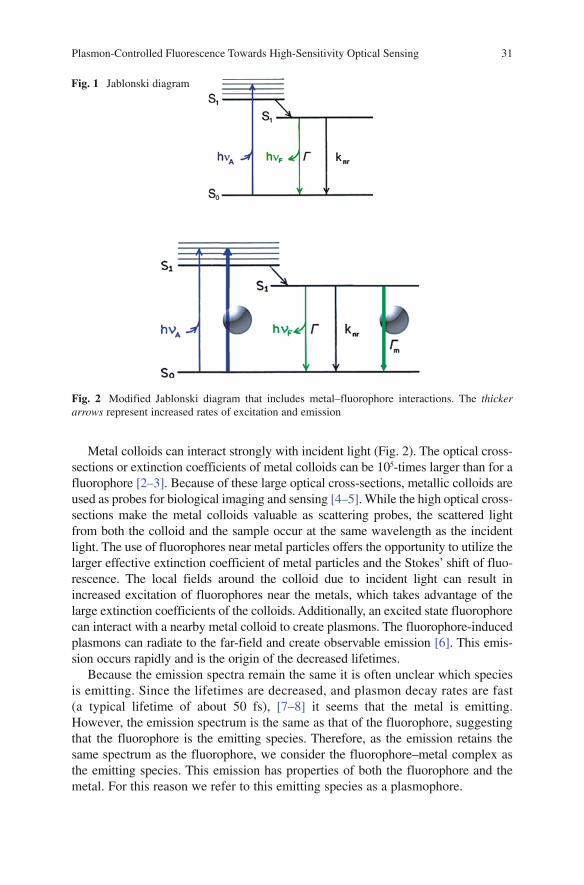
Plasmon-Controlled Fluorescence Towards High-Sensitivity Optical Sensing 31
Fig. 1 Jablonski diagram
Metal colloids can interact strongly with incident light (Fig. 2). The optical cross-sections or extinction coefficients of metal colloids can be 105-times larger than for a fluorophore [2–3]. Because of these large optical cross-sections, metallic colloids are used as probes for biological imaging and sensing [4–5]. While the high optical cross-sections make the metal colloids valuable as scattering probes, the scattered light from both the colloid and the sample occur at the same wavelength as the incident light. The use of fluorophores near metal particles offers the opportunity to utilize the larger effective extinction coefficient of metal particles and the Stokes’ shift of fluo-rescence. The local fields around the colloid due to incident light can result in increased excitation of fluorophores near the metals, which takes advantage of the large extinction coefficients of the colloids. Additionally, an excited state fluorophore can interact with a nearby metal colloid to create plasmons. The fluorophore-induced plasmons can radiate to the far-field and create observable emission [6]. This emis-sion occurs rapidly and is the origin of the decreased lifetimes.
Because the emission spectra remain the same it is often unclear which species is emitting. Since the lifetimes are decreased, and plasmon decay rates are fast (a typical lifetime of about 50 fs), [7–8] it seems that the metal is emitting. However, the emission spectrum is the same as that of the fluorophore, suggesting that the fluorophore is the emitting species. Therefore, as the emission retains the same spectrum as the fluorophore, we consider the fluorophore–metal complex as the emitting species. This emission has properties of both the fluorophore and the metal. For this reason we refer to this emitting species as a plasmophore.
Fig. 2 Modified Jablonski diagram that includes metal–fluorophore interactions. The thicker arrows represent increased rates of excitation and emission

32 K. Ray et al.
While we believe the emission is from the plasmophore, the effect of metals can be described from the perspective of the fluorophore. The quantum yield and life-time of a fluorophore are interrelated as defined below [9–10]:
0
nrk
ΓΦ =
Γ + (1)
0
nr
1
kτ =
Γ + (2)
where Γand knr are the radiative and nonradiative decay rates, respectively. In the
presence of metal, the quantum yield and lifetime are given by
m/m
m nrk
Γ + ΓΦ =
Γ + Γ + (3)
m
m n/
r
1
kτ =
Γ + Γ + (4)
where Γm and k
nr/ are radiative and nonradiative rates in the presence of metal
particles. Increases in radiative rates near metal particles result in increased quan-tum yields and decreased lifetimes. The modifications of k
nr by metal are assumed
to be negligible. The above equations result in the unusual prediction for fluoro-phore—metal interactions that the lifetime decreases as the intensity increases. A decrease in lifetime has several favorable consequences. Reduction in lifetime affords increased fluorophore photostability, as there is less time for excited state photodestructive processes to occur. Also, fluorophores can become less prone to optical saturation and have higher maximum emission rates. Thus, increase in emis-sion intensity accompanied by a decrease in lifetime results in increased detectabil-ity of single or multiple fluorophores.
2 Types of Metal–Fluorophore Interactions
Although metal—fluorophore interactions are based on the same physical princi-ples, the effects can be different based on the geometry of the metal structure. Figure 3 presents three possibilities: a fluorophore interacting with (1) metallic nanoparticles, (2) a smooth metal surface, and (3) a metal surface with a regular pattern. Metal particles can typically be used to increase the fluorescence intensi-ties. This increase occurs by a combination of enhanced fields around the metal and rapid and efficient plasmophore emission. These effects are usually called metal-enhanced fluorescence (MEF, Fig. 3, top panel), and typically result in increased intensities and decreased lifetimes.
The lower left panel (Fig. 3) shows a fluorophore interacting with a smooth metal film, typically about 40-nm thick silver, gold or 20-nm thick aluminum films. In this
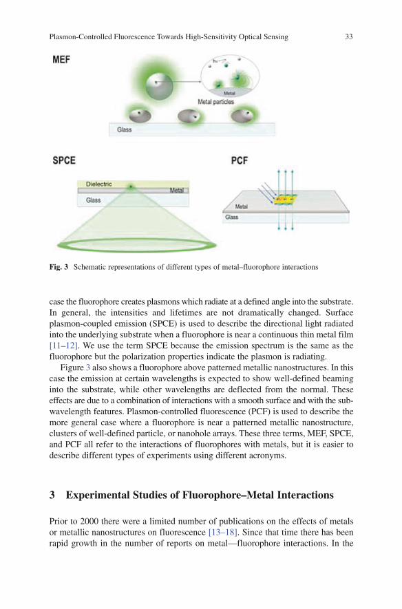
Plasmon-Controlled Fluorescence Towards High-Sensitivity Optical Sensing 33
case the fluorophore creates plasmons which radiate at a defined angle into the substrate. In general, the intensities and lifetimes are not dramatically changed. Surface plasmon-coupled emission (SPCE) is used to describe the directional light radiated into the underlying substrate when a fluorophore is near a continuous thin metal film [11–12]. We use the term SPCE because the emission spectrum is the same as the fluorophore but the polarization properties indicate the plasmon is radiating.
Figure 3 also shows a fluorophore above patterned metallic nanostructures. In this case the emission at certain wavelengths is expected to show well-defined beaming into the substrate, while other wavelengths are deflected from the normal. These effects are due to a combination of interactions with a smooth surface and with the sub-wavelength features. Plasmon-controlled fluorescence (PCF) is used to describe the more general case where a fluorophore is near a patterned metallic nanostructure, clusters of well-defined particle, or nanohole arrays. These three terms, MEF, SPCE, and PCF all refer to the interactions of fluorophores with metals, but it is easier to describe different types of experiments using different acronyms.
3 Experimental Studies of Fluorophore–Metal Interactions
Prior to 2000 there were a limited number of publications on the effects of metals or metallic nanostructures on fluorescence [13–18]. Since that time there has been rapid growth in the number of reports on metal—fluorophore interactions. In the
Fig. 3 Schematic representations of different types of metal–fluorophore interactions
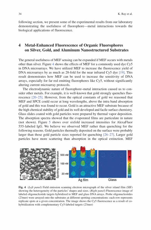
34 K. Ray et al.
following section, we present some of the experimental results from our laboratory demonstrating the usefulness of fluorophore—metal interactions towards the biological applications of fluorescence.
4 Metal-Enhanced Fluorescence of Organic Fluorophores on Silver, Gold, and Aluminum Nanostructured Substrates
The general usefulness of MEF sensing can be expanded if MEF occurs with metals other than silver. Figure 4 shows the effects of MEF for a commonly used dye Cy5 in DNA microarrays. We have utilized MEF to increase the fluorescence yield of DNA microarrays by as much as 28-fold for the near infrared Cy5 dye [19]. This result demonstrates how MEF can be used to increase the sensitivity of DNA arrays, especially for far red emitting fluorophores like Cy5, without significantly altering current microarray protocols.
The electrodynamic nature of fluorophore–metal interaction caused us to con-sider other metals. For example, it is well-known that gold strongly quenches fluo-rescence [20–25]. However, from the optical constants of gold we reasoned that MEF and SPCE could occur at long wavelengths, above the intra band absorption of gold and this was found to occur. Gold is an attractive MEF substrate because of the high chemical stability of gold and its well developed and facile surface chemistry. Glass slides coated with gold particles were prepared by thermal vapor deposition. The absorption spectra showed that the evaporated films are particulate in nature (not shown). Figure 5 shows over sixfold increased intensities for AlexaFluor 555-labeled IgG. We believe we observed MEF rather than quenching for the following reasons. Gold particles thermally deposited on the surface were probably larger than those gold particle sizes reported for quenching [26–27]. Larger gold particles have more scattering than absorption in the optical extinction. MEF
Fig. 4 (Left panel) Field emission scanning electron micrograph of the silver island film (SIF) showing the heterogeneity of the particles’ shapes and sizes. (Right panel) Fluorescence image of labeled oligonucleotide targets hybridized to MEF and glass DNA arrays. Probe oligonucleotides (23mer) were arrayed onto the substrates at different spotting concentrations: each row represents replicate spots at a given concentration. The image shows the Cy5 fluorescence as a result of co-hybridization with complementary Cy5-labeled targets (23mer)
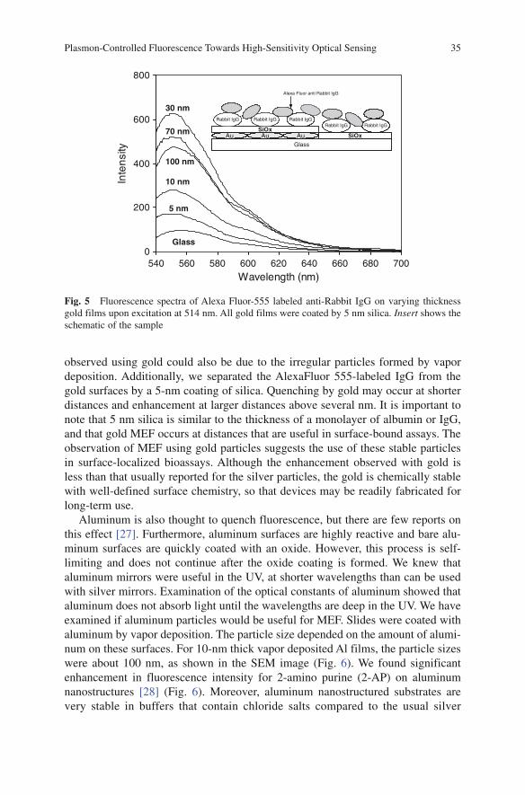
Plasmon-Controlled Fluorescence Towards High-Sensitivity Optical Sensing 35
observed using gold could also be due to the irregular particles formed by vapor deposition. Additionally, we separated the AlexaFluor 555-labeled IgG from the gold surfaces by a 5-nm coating of silica. Quenching by gold may occur at shorter distances and enhancement at larger distances above several nm. It is important to note that 5 nm silica is similar to the thickness of a monolayer of albumin or IgG, and that gold MEF occurs at distances that are useful in surface-bound assays. The observation of MEF using gold particles suggests the use of these stable particles in surface-localized bioassays. Although the enhancement observed with gold is less than that usually reported for the silver particles, the gold is chemically stable with well-defined surface chemistry, so that devices may be readily fabricated for long-term use.
Aluminum is also thought to quench fluorescence, but there are few reports on this effect [27]. Furthermore, aluminum surfaces are highly reactive and bare alu-minum surfaces are quickly coated with an oxide. However, this process is self-limiting and does not continue after the oxide coating is formed. We knew that aluminum mirrors were useful in the UV, at shorter wavelengths than can be used with silver mirrors. Examination of the optical constants of aluminum showed that aluminum does not absorb light until the wavelengths are deep in the UV. We have examined if aluminum particles would be useful for MEF. Slides were coated with aluminum by vapor deposition. The particle size depended on the amount of alumi-num on these surfaces. For 10-nm thick vapor deposited Al films, the particle sizes were about 100 nm, as shown in the SEM image (Fig. 6). We found significant enhancement in fluorescence intensity for 2-amino purine (2-AP) on aluminum nanostructures [28] (Fig. 6). Moreover, aluminum nanostructured substrates are very stable in buffers that contain chloride salts compared to the usual silver
Fig. 5 Fluorescence spectra of Alexa Fluor-555 labeled anti-Rabbit IgG on varying thickness gold films upon excitation at 514 nm. All gold films were coated by 5 nm silica. Insert shows the schematic of the sample
0
200
400
600
800
540 560 580 600 620 640 660 680 700
Wavelength (nm)
Inte
nsi
ty
Glass
5 nm
10 nm
100 nm
70 nm
30 nm
Glass
Alexa Fluor anti Rabbit IgG
Rabbit IgG Rabbit IgG Rabbit IgG
Rabbit IgG Rabbit IgG
Au Au Au
Rabbit IgG Rabbit IgG Rabbit IgGRabbit IgG
SiOxSiOx
Rabbit IgG Rabbit IgG
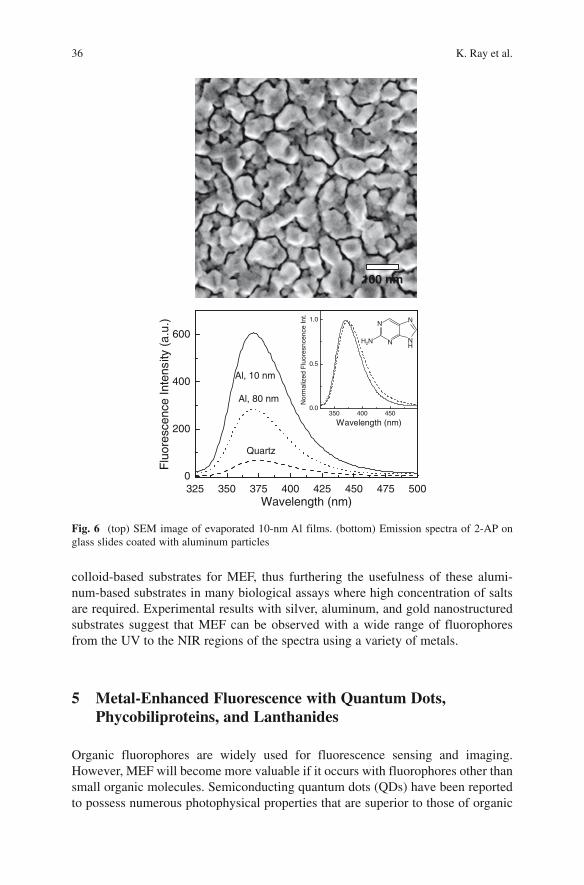
36 K. Ray et al.
colloid-based substrates for MEF, thus furthering the usefulness of these alumi-num-based substrates in many biological assays where high concentration of salts are required. Experimental results with silver, aluminum, and gold nanostructured substrates suggest that MEF can be observed with a wide range of fluorophores from the UV to the NIR regions of the spectra using a variety of metals.
5 Metal-Enhanced Fluorescence with Quantum Dots, Phycobiliproteins, and Lanthanides
Organic fluorophores are widely used for fluorescence sensing and imaging. However, MEF will become more valuable if it occurs with fluorophores other than small organic molecules. Semiconducting quantum dots (QDs) have been reported to possess numerous photophysical properties that are superior to those of organic
325 350 375 400 425 450 475 5000
200
400
600
350 400 4500.0
0.5
1.0
Flu
ores
cenc
e In
tens
ity (
a.u.
)
Wavelength (nm)
Nor
mal
ized
Flu
ores
ncen
ce In
t.
Wavelength (nm)
Quartz
Al, 80 nm
Al, 10 nm
N
N NH
N
H2N
100 nm
Fig. 6 (top) SEM image of evaporated 10-nm Al films. (bottom) Emission spectra of 2-AP on glass slides coated with aluminum particles
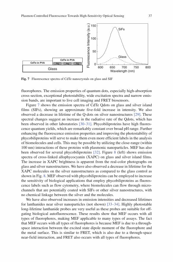
Plasmon-Controlled Fluorescence Towards High-Sensitivity Optical Sensing 37
fluorophores. The emission properties of quantum dots, especially high-absorption cross-section, exceptional photostability, wide excitation spectra and narrow emis-sion bands, are important to live cell imaging and FRET biosensors.
Figure 7 shows the emission spectra of CdTe Qdots on glass and silver island films (SIFs), showing an approximate five-fold increase in intensity. We also observed a decrease in lifetime of the Q-dots on silver nanostructures [29]. These spectral changes suggest an increase in the radiative rate of the Qdots, which has been observed in other laboratories [30–31]. Phycobiliproteins have high fluores-cence quantum yields, which are remarkably constant over broad pH range. Further enhancing the fluorescence emission properties and improving the photostability of phycobiliproteins will serve to make them even more efficient labels in the analysis of biomolecules and cells. This may be possible by utilizing the close-range (within 100 nm) interactions of these proteins with plasmonic nanoparticles. MEF has also been observed for several phycobiliproteins [32]. Figure 8 (left) shows emission spectra of cross-linked allophycocyanin (XAPC) on glass and silver island films. The increase in XAPC brightness is apparent from the real-color photographs on glass and silver nanostructures. We have also observed a decrease in lifetime for the XAPC molecules on the silver nanostructures as compared to the glass control as shown in Fig. 8. MEF observed with phycobiliproteins can be employed to increase the sensitivity of biological applications that employ phycobiliproteins as fluores-cence labels such as flow cytometry, where biomolecules can flow through micro-channels that are potentially coated with SIFs or other silver nanostructures, with no chemical linkage between the silver and the molecules.
We have also observed increases in emission intensities and decreased lifetimes for lanthanides near silver nanoparticles (not shown) [33–34]. Highly photostable long-lifetime lanthanide probes are very useful as these probes are suitable for off-gating biological autofluorescence. These results show that MEF occurs with all types of fluorophores, making MEF applicable to many types of assays. The fact that MEF occurs with all types of fluorophores is because MEF is due to a through-space interaction between the excited state dipole moment of the fluorophore and the metal surface. This is similar to FRET, which is also due to a through-space near-field interaction, and FRET also occurs with all types of fluorophores.
Fig. 7 Fluorescence spectra of CdTe nanocrystals on glass and SIF
600 650 700 750 8000
50
100
150
Flu
ores
cenc
e In
tens
ity (
a.u.
)
Wavelength (nm)
Glass
SiFs
Glass
AgCdTe in PVACdTe in PVA
Ag AgCdTe in PVA
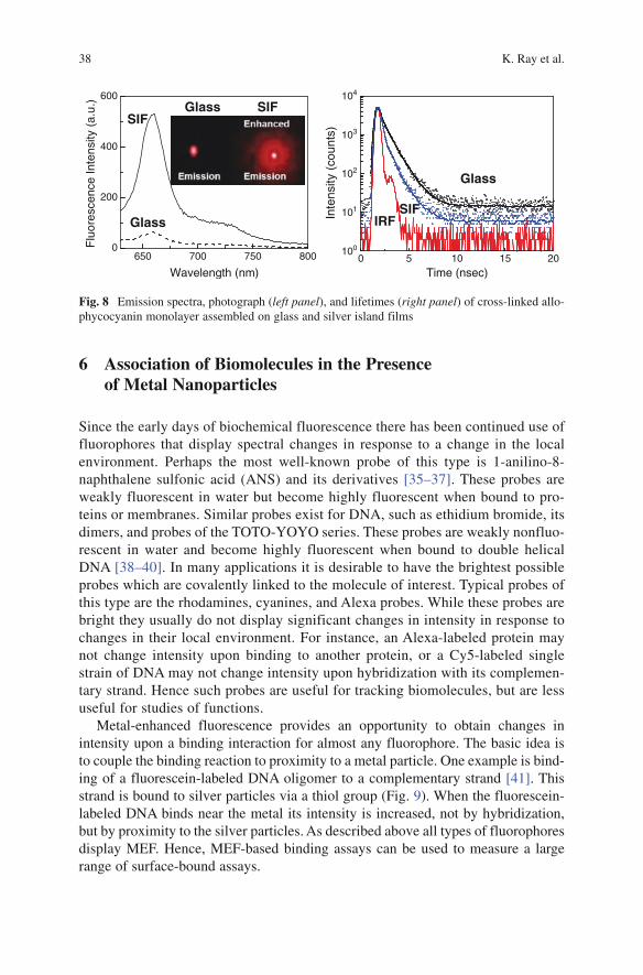
38 K. Ray et al.
6 Association of Biomolecules in the Presence of Metal Nanoparticles
Since the early days of biochemical fluorescence there has been continued use of fluorophores that display spectral changes in response to a change in the local environment. Perhaps the most well-known probe of this type is 1-anilino-8-naphthalene sulfonic acid (ANS) and its derivatives [35–37]. These probes are weakly fluorescent in water but become highly fluorescent when bound to pro-teins or membranes. Similar probes exist for DNA, such as ethidium bromide, its dimers, and probes of the TOTO-YOYO series. These probes are weakly nonfluo-rescent in water and become highly fluorescent when bound to double helical DNA [38–40]. In many applications it is desirable to have the brightest possible probes which are covalently linked to the molecule of interest. Typical probes of this type are the rhodamines, cyanines, and Alexa probes. While these probes are bright they usually do not display significant changes in intensity in response to changes in their local environment. For instance, an Alexa-labeled protein may not change intensity upon binding to another protein, or a Cy5-labeled single strain of DNA may not change intensity upon hybridization with its complemen-tary strand. Hence such probes are useful for tracking biomolecules, but are less useful for studies of functions.
Metal-enhanced fluorescence provides an opportunity to obtain changes in intensity upon a binding interaction for almost any fluorophore. The basic idea is to couple the binding reaction to proximity to a metal particle. One example is bind-ing of a fluorescein-labeled DNA oligomer to a complementary strand [41]. This strand is bound to silver particles via a thiol group (Fig. 9). When the fluorescein-labeled DNA binds near the metal its intensity is increased, not by hybridization, but by proximity to the silver particles. As described above all types of fluorophores display MEF. Hence, MEF-based binding assays can be used to measure a large range of surface-bound assays.
Fig. 8 Emission spectra, photograph (left panel), and lifetimes (right panel) of cross-linked allo-phycocyanin monolayer assembled on glass and silver island films
650 700 750 8000
200
400
600F
luor
esce
nce
Inte
nsity
(a.
u.)
Wavelength (nm)0 5 10 15 20
100
101
102
103
104
Inte
nsity
(co
unts
)
Time (nsec)
SIFGlassSIF
Glass
Glass
SIFIRF
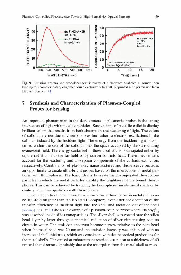
Plasmon-Controlled Fluorescence Towards High-Sensitivity Optical Sensing 39
7 Synthesis and Characterization of Plasmon-Coupled Probes for Sensing
An important phenomenon in the development of plasmonic probes is the strong interaction of light with metallic particles. Suspensions of metallic colloids display brilliant colors that results from both absorption and scattering of light. The colors of colloids are not due to chromophores but rather to electron oscillations in the colloids induced by the incident light. The energy from the incident light is con-tained within the size of the colloids plus the space occupied by the surrounding evanescent field. The energy contained in these oscillations is dissipated either by dipole radiation into the far-field or by conversion into heat. These mechanisms account for the scattering and absorption components of the colloids extinction, respectively. Combination of plasmonic nanostructures and fluorescence provides an opportunity to create ultra-bright probes based on the interactions of metal par-ticles with fluorophores. The basic idea is to create metal-conjugated fluorophore particles in which the metal particles amplify the brightness of the bound fluoro-phores. This can be achieved by trapping the fluorophores inside metal shells or by coating metal nanoparticles with fluorophores.
Recent theoretical calculations have shown that a fluorophore in metal shells can be 100-fold brighter than the isolated fluorophore, even after consideration of the transfer efficiency of incident light into the shell and radiation out of the shell [42–43]. Figure 10 shows an example of a plasmon-coupled probe where Ru(bpy)2+
3
was adsorbed inside silica nanoparticles. The silver shell was coated onto the silica bead layer by layer through a chemical reduction of silver nitrate using sodium citrate in water. The emission spectrum became narrow relative to the bare bead when the metal shell was 20 nm and the emission intensity was enhanced with an increase of shell thickness, which was consistent with the theoretical predictions for the metal shells. The emission enhancement reached saturation at a thickness of 40 nm and then decreased probably due to the absorption from the metal shell at wave-
Fig. 9 Emission spectra and time-dependent intensity of a fluorescein-labeled oligomer upon binding to a complementary oligomer bound exclusively to a SIF. Reprinted with permission from Elsevier Science [41]
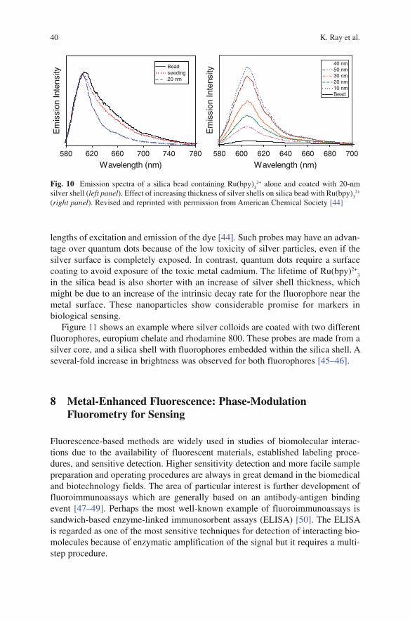
40 K. Ray et al.
lengths of excitation and emission of the dye [44]. Such probes may have an advan-tage over quantum dots because of the low toxicity of silver particles, even if the silver surface is completely exposed. In contrast, quantum dots require a surface coating to avoid exposure of the toxic metal cadmium. The lifetime of Ru(bpy)2+
3
in the silica bead is also shorter with an increase of silver shell thickness, which might be due to an increase of the intrinsic decay rate for the fluorophore near the metal surface. These nanoparticles show considerable promise for markers in biological sensing.
Figure 11 shows an example where silver colloids are coated with two different fluorophores, europium chelate and rhodamine 800. These probes are made from a silver core, and a silica shell with fluorophores embedded within the silica shell. A several-fold increase in brightness was observed for both fluorophores [45–46].
8 Metal-Enhanced Fluorescence: Phase-Modulation Fluorometry for Sensing
Fluorescence-based methods are widely used in studies of biomolecular interac-tions due to the availability of fluorescent materials, established labeling proce-dures, and sensitive detection. Higher sensitivity detection and more facile sample preparation and operating procedures are always in great demand in the biomedical and biotechnology fields. The area of particular interest is further development of fluoroimmunoassays which are generally based on an antibody-antigen binding event [47–49]. Perhaps the most well-known example of fluoroimmunoassays is sandwich-based enzyme-linked immunosorbent assays (ELISA) [50]. The ELISA is regarded as one of the most sensitive techniques for detection of interacting bio-molecules because of enzymatic amplification of the signal but it requires a multi-step procedure.
Fig. 10 Emission spectra of a silica bead containing Ru(bpy)32+ alone and coated with 20-nm
silver shell (left panel). Effect of increasing thickness of silver shells on silica bead with Ru(bpy)32+
(right panel). Revised and reprinted with permission from American Chemical Society [44]
0
580 620 660 700 740 780 580 600 620 640 660 680 700
Wavelength (nm)
Em
issi
on In
tens
ityBeadseeding20 nm
0
Wavelength (nm)
Em
issi
on In
tens
ity
40 nm50 nm30 nm20 nm10 nmBead
0
0
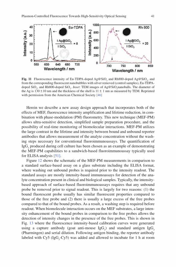
Plasmon-Controlled Fluorescence Towards High-Sensitivity Optical Sensing 41
Herein we describe a new assay design approach that incorporates both of the effects of MEF, fluorescence intensity amplification and lifetime reduction, in com-bination with phase-modulation (PM) fluorometry. This new technique (MEF-PM) allows ultra-sensitive detection, simplified sample preparation procedure, and the possibility of real-time monitoring of biomolecular interactions. MEF-PM utilizes the large contrast in the lifetime and intensity between bound and unbound reporter antibodies that allows measurement of the analyte concentration without the wash-ing steps necessary for conventional fluoroimmunoassays. The quantification of IgG
3 produced during cell culture has been chosen as an example of demonstrating
the MEF-PM capabilities to a sandwich-based fluoroimmunoassay typically used for ELISA analysis [51].
Figure 12 shows the schematic of the MEF-PM measurements in comparison to a standard surface-based assay on a glass substrate including the ELISA format, where washing out unbound probes is required prior to the intensity readout. The standard assays are mostly intensity-based immunoassays for detection of the ana-lyte concentration present in clinical and biological samples. Typically, the intensity-based approach of surface-based fluoroimmunoassays requires that any unbound probe be removed prior to signal readout. This is largely for two reasons: (1) the bound fluorescent probe usually has similar fluorescent properties compared to those of the free probe and (2) there is usually a large excess of the free probes compared to that of the bound probes. As a result, a washing step is required before readout. When biomolecule interaction occurs on the MEF substrates, a large inten-sity enhancement of the bound probes in comparison to the free probes allows the detection of intensity changes in the presence of the free probes. This is shown in Fig. 13 where the fluorescence intensity-based calibration curves were generated using a capture antibody (goat anti-mouse IgG
3) and standard antigen IgG
3
(Pharmingen) and serial dilution. Following antigen binding, the reporter antibody labeled with Cy5 (IgG
3-Cy5) was added and allowed to incubate for 1 h at room
Fig. 11 Fluorescence intensity of Eu-TDPA-doped Ag@SiO2 and Rh880-doped Ag@SiO
2, and
from the corresponding fluorescent nanobubbles with silver removed (control samples), Eu-TDPA-doped SiO
2, and Rh800-doped SiO
2. Inset: TEM images of Ag@SiO
2nanoballs. The diameter of
the Ag is 130 +- 10 nm and the thickness of the shell is 11 +- 1 nm as measured by TEM. Reprinted with permission from the American Chemical Society [46]

42 K. Ray et al.
temperature. After incubation, the fluorescence intensity was measured in the pres-ence of free probes on the MEF substrates. A control experiment was carried out on bare glass where unbound probes were washed out. The four-parameter logistic function was used which is recognized as the reference standard for fitting the mean concentration-response for immunoassays [52].
The clear advantage of the MEF-based assay is that there is no requirement for washing out unbound probes prior to readout and a substantial increase in the fluo-rescence signal. These two advantages led to a shortening of the procedures and to increased accuracy, which are important aspects in performing measurements as rapidly as possible with potential for real-time monitoring of bioprocess samples and binding interactions. Note that both calibration curves display a similar dynamic range for analyte concentration as can be judged by the midpoint values
Fig. 12 Schematics of sandwich assays for the detection of IgG3 on glass, MEF substrates (silver island film), and using ELISA. Note that detection of IgG
3 on glass and using ELISA requires
washing out the unbound probes while on MEF substrates. The readout is in the presence of unbound probes
Excitation
Glass substrate MEF Substrate MEF substrate
Emission
Ag
ELISA
Capture antibody
Antibody-Cy5
Antibody-AP
Blocking Molecule
Antigen, IgG3
Fig. 13 Intensity-based Calibration Curves For IgG3 immunoassays using glass and MEF sub-
strates. The intensity readouts were performed in the presence of free probes (4 μg ml−1) for the MEF substrate and after washing out for the glass
0.1 1 10 100 1000 100000
10
20
200
400
600
800
1000
1200
Inte
nsity
IgG3 [ng / ml]
MEF 351.5±13.8 ng / ml
Glass274.9±26.3 ng/ml
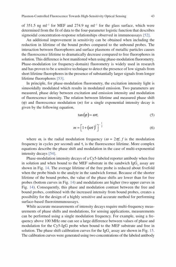
Plasmon-Controlled Fluorescence Towards High-Sensitivity Optical Sensing 43
of 351.5 ng ml−1 for MEF and 274.9 ng ml−1 for the glass surface, which were determined from the fit of data to the four-parameter logistic function that describes sigmoidal concentration-response relationships observed in immunoassays [52].
An additional improvement in sensitivity can be obtained when including the reduction in lifetime of the bound probes compared to the unbound probes. The interaction between fluorophores and surface plasmons of metallic particles causes the fluorescence lifetime to dramatically decrease compared to free fluorophores in solution. This difference is best manifested when using phase-modulation fluorometry. Phase-modulation (or frequency-domain) fluorometry is widely used in research and has proven to be a sensitive technique to detect the presence of low signals from short lifetime fluorophores in the presence of substantially larger signals from longer lifetime fluorophores [53].
In principle, for phase-modulation fluorometry, the excitation intensity light is sinusoidally modulated which results in modulated emission. Two parameters are measured, phase delay between excitation and emission intensity and modulation of fluorescence intensity. The relation between lifetime and measured phase shift (ϕ) and fluorescence modulation (m) for a single exponential intensity decay is given by the following equation,
( )tan j wt,= (5)
( )1
2 21m wt−
= + (6)
where w, is the radial modulation frequency (w = 2pf, f is the modulation frequency in cycles per second) and τ, is the fluorescence lifetime. More complex equations describe the phase shift and modulation in the case of multi-exponential intensity decays [54].
Phase-modulation intensity decays of a Cy5-labeled reporter antibody when free in solution and when bound to the MEF substrate in the sandwich IgG
3 assay are
shown in Fig. 14. The average lifetime of the free probe is reduced about fivefold when the probe binds to the analyte in the sandwich format. Because of the shorter lifetime of the bound probes, the value of the phase shifts are lower than for free probes (bottom curves in Fig. 14) and modulations are higher (two upper curves in Fig. 14). Consequently, this phase and modulation contrast between the free and bound probes, combined with the increased intensity from bound probes, creates a possibility for the design of a highly sensitive and accurate method for performing surface-based fluoroimmunoassays.
While accurate measurements of intensity decays require multi-frequency meas-urements of phase shifts and modulations, for sensing applications, measurements can be performed using a single modulation frequency. For example, using a fre-quency above 100 MHz one can see a large difference between values of phase and modulation for the Cy5-IgG probe when bound to the MEF substrate and free in solution. The phase shift calibration curves for the IgG
3 assay are shown in Fig. 15.
The calibration curves were generated using two concentrations of the labeled antibody
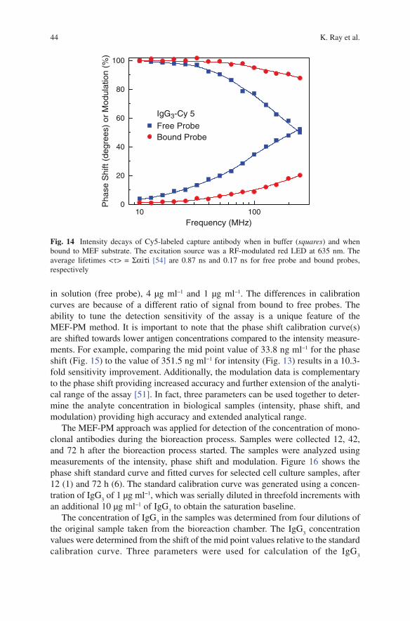
44 K. Ray et al.
in solution (free probe), 4 μg ml−1 and 1 μg ml−1. The differences in calibration curves are because of a different ratio of signal from bound to free probes. The ability to tune the detection sensitivity of the assay is a unique feature of the MEF-PM method. It is important to note that the phase shift calibration curve(s) are shifted towards lower antigen concentrations compared to the intensity measure-ments. For example, comparing the mid point value of 33.8 ng ml−1 for the phase shift (Fig. 15) to the value of 351.5 ng ml−1 for intensity (Fig. 13) results in a 10.3-fold sensitivity improvement. Additionally, the modulation data is complementary to the phase shift providing increased accuracy and further extension of the analyti-cal range of the assay [51]. In fact, three parameters can be used together to deter-mine the analyte concentration in biological samples (intensity, phase shift, and modulation) providing high accuracy and extended analytical range.
The MEF-PM approach was applied for detection of the concentration of mono-clonal antibodies during the bioreaction process. Samples were collected 12, 42, and 72 h after the bioreaction process started. The samples were analyzed using measurements of the intensity, phase shift and modulation. Figure 16 shows the phase shift standard curve and fitted curves for selected cell culture samples, after 12 (1) and 72 h (6). The standard calibration curve was generated using a concen-tration of IgG
3 of 1 μg ml−1, which was serially diluted in threefold increments with
an additional 10 μg ml−1 of IgG3 to obtain the saturation baseline.
The concentration of IgG3 in the samples was determined from four dilutions of
the original sample taken from the bioreaction chamber. The IgG3 concentration
values were determined from the shift of the mid point values relative to the standard calibration curve. Three parameters were used for calculation of the IgG
3
Fig. 14 Intensity decays of Cy5-labeled capture antibody when in buffer (squares) and when bound to MEF substrate. The excitation source was a RF-modulated red LED at 635 nm. The average lifetimes <t> = Σαiτi [54] are 0.87 ns and 0.17 ns for free probe and bound probes, respectively
10 1000
20
40
60
80
100
Pha
se S
hift
(deg
rees
) or
Mod
ulat
ion
(%)
Frequency (MHz)
IgG3-Cy 5
Free ProbeBound Probe

Plasmon-Controlled Fluorescence Towards High-Sensitivity Optical Sensing 45
Fig. 15 Phase calibration curves for IgG3 immunoassay at two concentrations of free probes, 4 μg ml−1 and 1 μg ml−1. The excitation was a red LED (635 nm) modulated at a frequency of 155 MHz
0.01 0.1 1 10 100 1000 1000010
15
20
25
30
35
40
45
[IgG3−Cy5] 1 ug / ml:33.8±4.1 ng / ml
[IgG3−Cy5] 4 ug/ml:150.9±13.5 ng/ml
Pha
se S
hift
(Deg
rees
)
IgG3 [ng / ml]
concentrations, phase shifts as shown in Fig. 16, modulations, and intensities (plots not shown). In parallel, concentrations of the IgG
3 were determined using an
ELISA technique. Very good agreement between ELISA and MEF-PM values was found for the selected samples (Table 1). The average values for ELISA were determined from duplicate samples, while the average values for MEF-PM were determined from triplicate measurements of intensity, phase shift, and modulation as shown in Table 1 for each parameter measured. The larger variations of the
Fig. 16 Phase shift plots for standards and cell culture samples. The detection antibody concen-tration was 4 μg ml−1
0.1 1 10 100 1000 1000015
20
25
30
35
40
45
a
StandardSample 1Sample 6
Pha
se S
hift
(Deg
rees
)
Dilution Fold

46 K. Ray et al.
MEF-PM values compared to ELISA can be attributed to nonoptimized MEF substrates.
Further optimization in the preparation of MEF substrates, surface chemistry, and choice of fluorophore can be expected which will lead to enhanced sensitivity to about 100-fold compared to the conventional intensity-based assays. Additionally, low-cost LED-based phase-modulation instrumentation has already been demon-strated for similar measurements [55]. These advances open the door for compact benchtop or handheld instruments similar to those routinely used for glucose moni-toring in a bioprocessing lab.
9 Surface Plasmon-Coupled Emission (SPCE)
In the previous sections we discussed the effects of metallic particles on fluoro-phores. We now consider the interactions of fluorophores with continuous metal films. Although the underlying electrodynamics mechanisms are the same for the interactions of fluorophores with metal particles or surfaces, the effects on fluores-cence are very different. These differences arise from the defined geometry of a metal film and from the different nature of surface plasmons on sub-wavelength size particles and on planar surfaces. Surface plasmon-coupled emission (SPCE) is a phenomenon that occurs with excited fluorophores near continuous metallic surfaces covered with thin (~50 nm) metal films. These films are visually almost completely opaque. Excited fluorophores within about 100 nm of the surface result in strongly directional emission through the metal film and into the substrate. A large fraction of the total light energy is coupled into the substrate. This remarkable phenomenon is the result of near-field interactions of the excited fluorophores with the thin metal film, and is not simply a reflective or transmissive phenomenon. The SPCE emission is highly directional and appears at a well-defined angle. The emission spectrum is the same as that of the fluorophores, yet the emission is completely p-polarized.
A typical configuration for a SPCE experiment is shown in Fig. 17. We exam-ined the fluorophore contained in a thin layer of polyvinyl alcohol (PVA) on a thin metal film. The sample was placed on a hemicylindrical prism and excited from the sample side of the prism (Fig. 17). In this case, the fluorophores are excited from the air side of the sample and the emission is observed on the distal glass side of
Table 1 Concentrations of IgG3 in cell culture samples determined using the multiple analysis
parameters of the MEF-PM method and ELISA
Sample # 1 3 6
ELISA 5.84 ± 0.28 12.60 ± 0.34 32.44 ± 2.14Intensity 5.18 ± 0.73 9.55 ± 1.23 35.83 ± 4.28Phase 5.97 ± 0.71 14.72 ± 1.53 30.77 ± 5.60Modulation 5.58 ± 1.17 10.87 ± 0.53 33.45 ± 1.19

Plasmon-Controlled Fluorescence Towards High-Sensitivity Optical Sensing 47
the substrate. This is called the reverse Kretschmann (RK) configuration. Plasmons are not created on the metal surface by the light incident from this direction. For typical three-dimensional samples, not on a metal film, the emission is mostly the same in all directions (isotropic emission). In contrast, the fluorophores above the metal film yield a cone of emission into the substrate (Fig. 18). This means that almost all the emission into the substrate occurs at a defined angle θ
F relative to the
normal axis. This result is even more remarkable when considering the optical properties of the metal films. These films are highly reflective and are visually almost opaque. SPCE is also observed with aluminum and gold (as shown in Fig. 18), which is surprising because both gold and aluminum are known to strongly quench fluorescence as discussed earlier.
Excited fluorophores in the near-field could create plasmons in the metal film, and these plasmons in turn radiate into the substrate [11–12]. Analytical theories have been developed for explaining SPCE [56–57]. An intuitive understanding of SPCE can be obtained from the principles of surface plasmon resonance (SPR) [58–63].
If SPCE displays the same characteristics as SPR, then fluorophores near the metal film will emit into the prism at angles defined by the emission wavelength and by the optical properties of the metal at the emission wavelength. We have observed the longer wavelength Stokes’ shifted emission to occur at smaller angles. This separation of wavelength has been observed for fluorophores on silver films as shown in Fig. 19. This result shows that a simple metal film can be used to create directional emission and to separate different wavelengths. The wavelength depend-ence of SPR and SPCE results from the wavelength dependence of the optical constants of the metals.
Plasmon-coupled emission displays interesting polarization properties. SPR only occurs for the p-polarized component of the incident light because the pro-jected wavevector of this component on the metal plane depends on the incident
Fig. 17 Surface plasmon-coupled emission set up
Notch Filter
Long pass Filter
Spectrophotometer
Sample
Hemicylindrical prism
Fiber
SPCE
λex

48 K. Ray et al.
angle. Hence, SPCE is expected to be p-polarized at all angles around the cone, independently of the mode of excitation. The p-polarization of SPR and SPCE leads to the impression that only dipole measurements perpendicular to the metal surface will couple with the metal and cause SPCE. From the far-field the dipoles oriented perpendicular will result in p-polarized fields on the metal. However, the situation may be different for near-field interactions of the fluorophore with the metal surface, and we can expect to see coupling of fluorophores, parallel to the metal surface.
There are a number of publications on the theoretical aspects of fluorophores interacting with smooth metallic surfaces or mirrors [64–70]. This theory mostly describes fluorophores on or near thick metal films or mirrors. According to these papers there appears to be three possible processes for fluorophores near a smooth metal surface. The fluorophore can be quenched, can couple to surface plasmons or can emit into free-space. If the fluorophore is close to the surface (d < 10 nm) there is a high rate for radiationless deactivation and the emission appears to be quenched. At longer distances the reflected field interferes constructively or destructively, resulting in the oscillatory behavior reported for fluorophores in front of mirrors [68]. At distances from 20 to 100 nm the dominant decay rate is expected to be due to the surface plasmons. The coupling of fluorophores over these longer distances explains why gold films can also be used to couple emission into the prism. Forster transfer to the gold surface is likely to be minimal at distances above 10 nm where SPCE is still efficient. This is important for the applications of SPCE because cou-pling will occur over a significant volume in the sample allowing detection of lower overall analyte concentrations. In addition, larger depths for SPCE allows for con-struction of bioassays with multiple layers of proteins or the use of a separation layer to protect the metallic layer against corrosion and adverse chemical reactions.
During the past several years there have been an increased number of publica-tions on SPCE to develop both a basic understanding of the phenomenon and to use SPCE for sensing applications [71–74]. Here we have chosen a few examples which illustrate the general features of SPCE and its applications. An important feature of SPCE is the distances over which the fluorophores can couple to surface
Fig. 18 Cone of emission for different fluorophores in PVA on aluminum (left), silver (middle), and gold (right) films
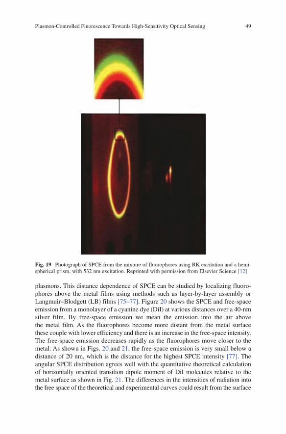
Plasmon-Controlled Fluorescence Towards High-Sensitivity Optical Sensing 49
plasmons. This distance dependence of SPCE can be studied by localizing fluoro-phores above the metal films using methods such as layer-by-layer assembly or Langmuir–Blodgett (LB) films [75–77]. Figure 20 shows the SPCE and free-space emission from a monolayer of a cyanine dye (DiI) at various distances over a 40-nm silver film. By free-space emission we mean the emission into the air above the metal film. As the fluorophores become more distant from the metal surface these couple with lower efficiency and there is an increase in the free-space intensity. The free-space emission decreases rapidly as the fluorophores move closer to the metal. As shown in Figs. 20 and 21, the free-space emission is very small below a distance of 20 nm, which is the distance for the highest SPCE intensity [77]. The angular SPCE distribution agrees well with the quantitative theoretical calculation of horizontally oriented transition dipole moment of DiI molecules relative to the metal surface as shown in Fig. 21. The differences in the intensities of radiation into the free space of the theoretical and experimental curves could result from the surface
Fig. 19 Photograph of SPCE from the mixture of fluorophores using RK excitation and a hemi-spherical prism, with 532 nm excitation. Reprinted with permission from Elsevier Science [12]
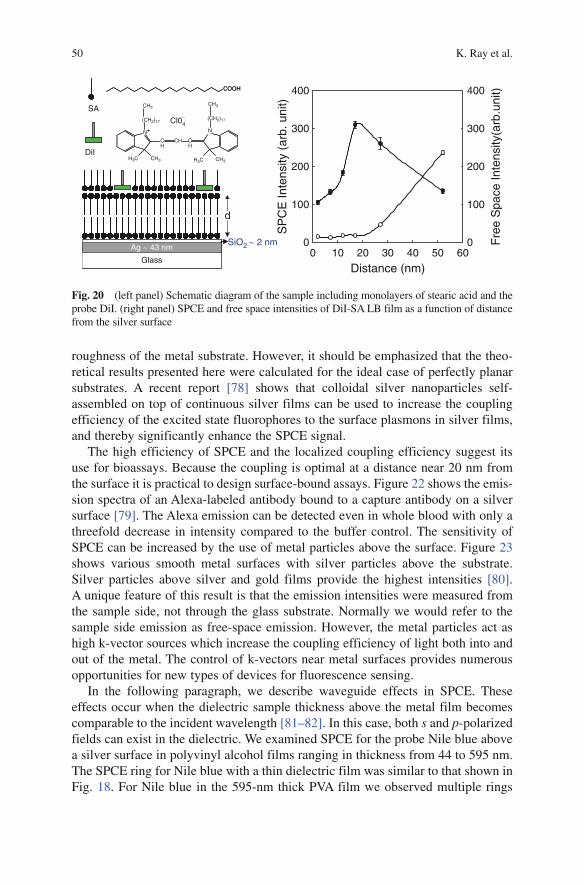
50 K. Ray et al.
roughness of the metal substrate. However, it should be emphasized that the theo-retical results presented here were calculated for the ideal case of perfectly planar substrates. A recent report [78] shows that colloidal silver nanoparticles self-assembled on top of continuous silver films can be used to increase the coupling efficiency of the excited state fluorophores to the surface plasmons in silver films, and thereby significantly enhance the SPCE signal.
The high efficiency of SPCE and the localized coupling efficiency suggest its use for bioassays. Because the coupling is optimal at a distance near 20 nm from the surface it is practical to design surface-bound assays. Figure 22 shows the emis-sion spectra of an Alexa-labeled antibody bound to a capture antibody on a silver surface [79]. The Alexa emission can be detected even in whole blood with only a threefold decrease in intensity compared to the buffer control. The sensitivity of SPCE can be increased by the use of metal particles above the surface. Figure 23 shows various smooth metal surfaces with silver particles above the substrate. Silver particles above silver and gold films provide the highest intensities [80]. A unique feature of this result is that the emission intensities were measured from the sample side, not through the glass substrate. Normally we would refer to the sample side emission as free-space emission. However, the metal particles act as high k-vector sources which increase the coupling efficiency of light both into and out of the metal. The control of k-vectors near metal surfaces provides numerous opportunities for new types of devices for fluorescence sensing.
In the following paragraph, we describe waveguide effects in SPCE. These effects occur when the dielectric sample thickness above the metal film becomes comparable to the incident wavelength [81–82]. In this case, both s and p-polarized fields can exist in the dielectric. We examined SPCE for the probe Nile blue above a silver surface in polyvinyl alcohol films ranging in thickness from 44 to 595 nm. The SPCE ring for Nile blue with a thin dielectric film was similar to that shown in Fig. 18. For Nile blue in the 595-nm thick PVA film we observed multiple rings
Fig. 20 (left panel) Schematic diagram of the sample including monolayers of stearic acid and the probe DiI. (right panel) SPCE and free space intensities of DiI-SA LB film as a function of distance from the silver surface
Ag ~ 43 nm
COOH
SA
DiI
N
CH3
Ag ~ 43 nm
Glass
Ag ~ 43 nmSiO2 ~ 2 nm
COOH
d
N
CH CH
CH
(CH2)17
CH3
(CH2)17
CH3
H3C CH3
Cl0−4
H3C
Distance (nm)0 10 20 30 40 50 60
SP
CE
Inte
nsity
(ar
b. u
nit)
0
100
200
300
400
Fre
e S
pace
Inte
nsity
(arb
.uni
t)
0
100
200
300
400
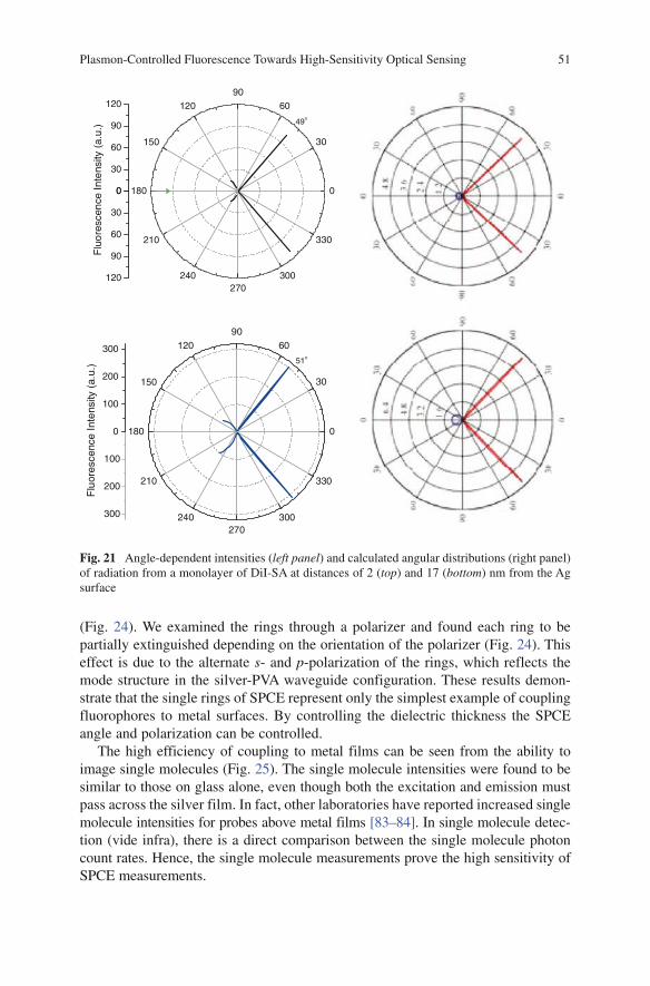
Plasmon-Controlled Fluorescence Towards High-Sensitivity Optical Sensing 51
(Fig. 24). We examined the rings through a polarizer and found each ring to be partially extinguished depending on the orientation of the polarizer (Fig. 24). This effect is due to the alternate s- and p-polarization of the rings, which reflects the mode structure in the silver-PVA waveguide configuration. These results demon-strate that the single rings of SPCE represent only the simplest example of coupling fluorophores to metal surfaces. By controlling the dielectric thickness the SPCE angle and polarization can be controlled.
The high efficiency of coupling to metal films can be seen from the ability to image single molecules (Fig. 25). The single molecule intensities were found to be similar to those on glass alone, even though both the excitation and emission must pass across the silver film. In fact, other laboratories have reported increased single molecule intensities for probes above metal films [83–84]. In single molecule detec-tion (vide infra), there is a direct comparison between the single molecule photon count rates. Hence, the single molecule measurements prove the high sensitivity of SPCE measurements.
Fig. 21 Angle-dependent intensities (left panel) and calculated angular distributions (right panel) of radiation from a monolayer of DiI-SA at distances of 2 (top) and 17 (bottom) nm from the Ag surface
0
30
6090
120
150
180
210
240270
300
330
0
100
200
300
100
200
300
Flu
ores
cenc
e In
tens
ity (
a.u.
) 51o
0
30
6090
120
150
180
210
240270
300
330
0
30
60
90
120
0
30
60
90
120
Flu
ores
cenc
e In
tens
ity (
a.u.
) 49o

52 K. Ray et al.
Fig. 22 Fluorescence spectra (SPCE) of the AlexaFluor 647-labeled anti-rabbit antibodies bound to the rabbit IgG immobilized on a 50-nm silver mirror surface observed in buffer, human serum, and human whole blood (Kretschmann (KR) configuration) [79]. Reprinted with permission from Elsevier Science
Fig. 23 Left: Schematic of substrates with silver particles above a smooth metal film. Each sub-strate has silver particles on the silica. Right: Emission spectra of AlexaFluor555-labeled IgG on the substrates. Revised from [80]. With permission from Elsevier Science
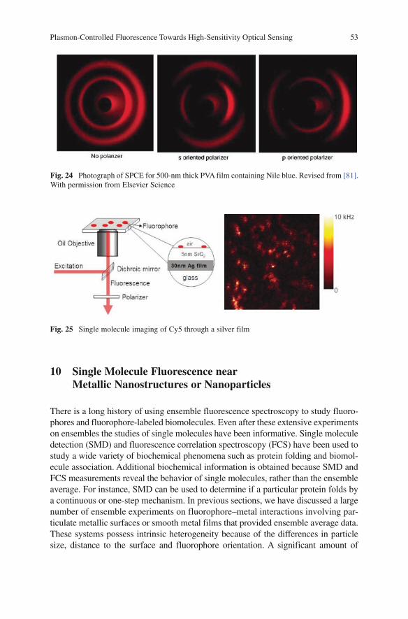
Plasmon-Controlled Fluorescence Towards High-Sensitivity Optical Sensing 53
10 Single Molecule Fluorescence near Metallic Nanostructures or Nanoparticles
There is a long history of using ensemble fluorescence spectroscopy to study fluoro-phores and fluorophore-labeled biomolecules. Even after these extensive experiments on ensembles the studies of single molecules have been informative. Single molecule detection (SMD) and fluorescence correlation spectroscopy (FCS) have been used to study a wide variety of biochemical phenomena such as protein folding and biomol-ecule association. Additional biochemical information is obtained because SMD and FCS measurements reveal the behavior of single molecules, rather than the ensemble average. For instance, SMD can be used to determine if a particular protein folds by a continuous or one-step mechanism. In previous sections, we have discussed a large number of ensemble experiments on fluorophore–metal interactions involving par-ticulate metallic surfaces or smooth metal films that provided ensemble average data. These systems possess intrinsic heterogeneity because of the differences in particle size, distance to the surface and fluorophore orientation. A significant amount of
Fig. 24 Photograph of SPCE for 500-nm thick PVA film containing Nile blue. Revised from [81]. With permission from Elsevier Science
Fig. 25 Single molecule imaging of Cy5 through a silver film
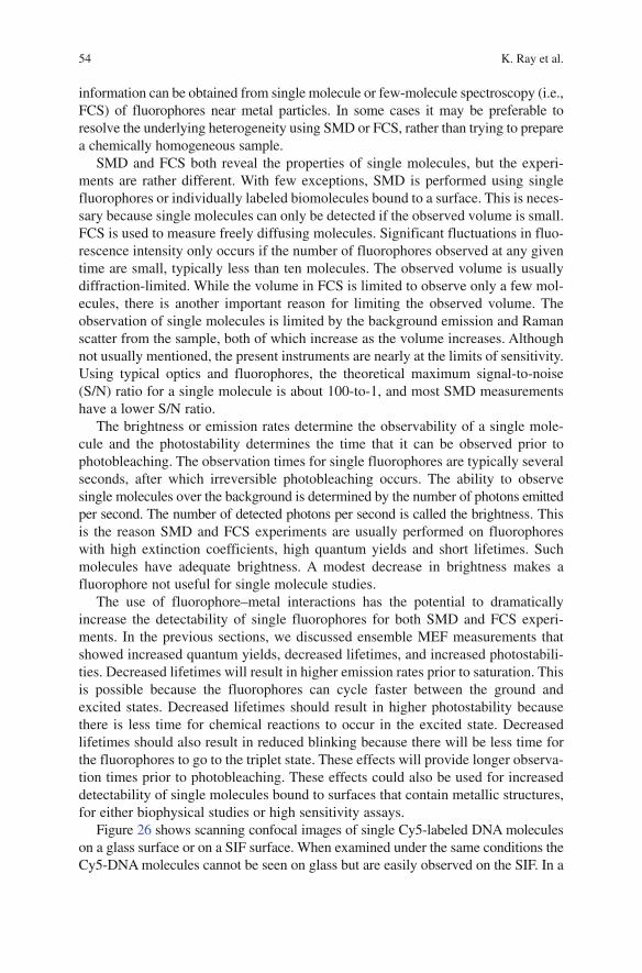
54 K. Ray et al.
information can be obtained from single molecule or few-molecule spectroscopy (i.e., FCS) of fluorophores near metal particles. In some cases it may be preferable to resolve the underlying heterogeneity using SMD or FCS, rather than trying to prepare a chemically homogeneous sample.
SMD and FCS both reveal the properties of single molecules, but the experi-ments are rather different. With few exceptions, SMD is performed using single fluorophores or individually labeled biomolecules bound to a surface. This is neces-sary because single molecules can only be detected if the observed volume is small. FCS is used to measure freely diffusing molecules. Significant fluctuations in fluo-rescence intensity only occurs if the number of fluorophores observed at any given time are small, typically less than ten molecules. The observed volume is usually diffraction-limited. While the volume in FCS is limited to observe only a few mol-ecules, there is another important reason for limiting the observed volume. The observation of single molecules is limited by the background emission and Raman scatter from the sample, both of which increase as the volume increases. Although not usually mentioned, the present instruments are nearly at the limits of sensitivity. Using typical optics and fluorophores, the theoretical maximum signal-to-noise (S/N) ratio for a single molecule is about 100-to-1, and most SMD measurements have a lower S/N ratio.
The brightness or emission rates determine the observability of a single mole-cule and the photostability determines the time that it can be observed prior to photobleaching. The observation times for single fluorophores are typically several seconds, after which irreversible photobleaching occurs. The ability to observe single molecules over the background is determined by the number of photons emitted per second. The number of detected photons per second is called the brightness. This is the reason SMD and FCS experiments are usually performed on fluorophores with high extinction coefficients, high quantum yields and short lifetimes. Such molecules have adequate brightness. A modest decrease in brightness makes a fluorophore not useful for single molecule studies.
The use of fluorophore–metal interactions has the potential to dramatically increase the detectability of single fluorophores for both SMD and FCS experi-ments. In the previous sections, we discussed ensemble MEF measurements that showed increased quantum yields, decreased lifetimes, and increased photostabili-ties. Decreased lifetimes will result in higher emission rates prior to saturation. This is possible because the fluorophores can cycle faster between the ground and excited states. Decreased lifetimes should result in higher photostability because there is less time for chemical reactions to occur in the excited state. Decreased lifetimes should also result in reduced blinking because there will be less time for the fluorophores to go to the triplet state. These effects will provide longer observa-tion times prior to photobleaching. These effects could also be used for increased detectability of single molecules bound to surfaces that contain metallic structures, for either biophysical studies or high sensitivity assays.
Figure 26 shows scanning confocal images of single Cy5-labeled DNA molecules on a glass surface or on a SIF surface. When examined under the same conditions the Cy5-DNA molecules cannot be seen on glass but are easily observed on the SIF. In a
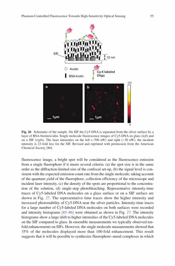
Plasmon-Controlled Fluorescence Towards High-Sensitivity Optical Sensing 55
fluorescence image, a bright spot will be considered as the fluorescence emission from a single fluorophore if it meets several criteria: (a) the spot size is in the same order as the diffraction-limited size of the confocal set-up, (b) the signal level is con-sistent with the expected emission count rate from the single molecule, taking account of the quantum yield of the fluorophore, collection efficiency of the microscope and incident laser intensity, (c) the density of the spots are proportional to the concentra-tion of the solution, (d) single-step photobleaching. Representative intensity-time traces of Cy5-labeled DNA molecules on a glass surface or on a SIF surface are shown in Fig. 27. The representative time traces show the higher intensity and increased photostability of Cy5-DNA near the silver particles. Intensity-time traces for a large number of Cy5-labeled DNA molecules on both surfaces were recorded and intensity histograms [85–86] were obtained as shown in Fig. 27. The intensity histograms show a large shift to higher intensities of the Cy5-labeled DNA molecules on the SIF compared to glass. In ensemble measurements we typically observed ten-fold enhancements on SIFs. However, the single molecule measurements showed that 35% of the molecules displayed more than 100-fold enhancement. This result suggests that it will be possible to synthesize fluorophore–metal complexes in which
Fig. 26 Schematic of the sample. On SIF the Cy5-DNA is separated from the silver surface by a layer of BSA-biotin/avidin. Single molecule fluorescence images of Cy5-DNA on glass (left) and on a SIF (right). The laser intensities on the left (−700 nW) and right (−30 nW), the incident intensity is 23-fold less for the SIF. Revised and reprinted with permission from the American Chemical Society [86]
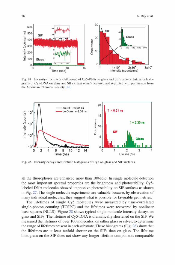
56 K. Ray et al.
Fig. 27 Intensity-time traces (left panel) of Cy5-DNA on glass and SIF surfaces. Intensity histo-grams of Cy5-DNA on glass and SIFs (right panel). Revised and reprinted with permission from the American Chemical Society [86]
Fig. 28 Intensity decays and lifetime histograms of Cy5 on glass and SIF surfaces
all the fluorophores are enhanced more than 100-fold. In single molecule detection the most important spectral properties are the brightness and photostability. Cy5-labeled DNA molecules showed impressive photostability on SIF surfaces as shown in Fig. 27. The single molecule experiments are valuable because, by observation of many individual molecules, they suggest what is possible for favorable geometries.
The lifetimes of single Cy5 molecules were measured by time-correlated single-photon counting (TCSPC) and the lifetimes were recovered by nonlinear least-squares (NLLS). Figure 28 shows typical single molecule intensity decays on glass and SIFs. The lifetime of Cy5-DNA is dramatically shortened on the SIF. We measured the lifetimes of over 100 molecules, on either glass or silver, to determine the range of lifetimes present in each substrate. These histograms (Fig. 28) show that the lifetimes are at least tenfold shorter on the SIFs than on glass. The lifetime histogram on the SIF does not show any longer lifetime components comparable
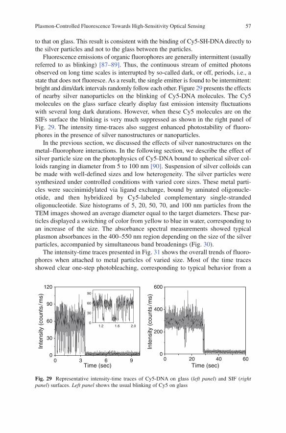
Plasmon-Controlled Fluorescence Towards High-Sensitivity Optical Sensing 57
to that on glass. This result is consistent with the binding of Cy5-SH-DNA directly to the silver particles and not to the glass between the particles.
Fluorescence emissions of organic fluorophores are generally intermittent (usually referred to as blinking) [87–89]. Thus, the continuous stream of emitted photons observed on long time scales is interrupted by so-called dark, or off, periods, i.e., a state that does not fluoresce. As a result, the single emitter is found to be intermittent: bright and dim/dark intervals randomly follow each other. Figure 29 presents the effects of nearby silver nanoparticles on the blinking of Cy5-DNA molecules. The Cy5 molecules on the glass surface clearly display fast emission intensity fluctuations with several long dark durations. However, when these Cy5 molecules are on the SIFs surface the blinking is very much suppressed as shown in the right panel of Fig. 29. The intensity time-traces also suggest enhanced photostability of fluoro-phores in the presence of silver nanostructures or nanoparticles.
In the previous section, we discussed the effects of silver nanostructures on the metal–fluorophore interactions. In the following section, we describe the effect of silver particle size on the photophysics of Cy5-DNA bound to spherical silver col-loids ranging in diameter from 5 to 100 nm [90]. Suspension of silver colloids can be made with well-defined sizes and low heterogeneity. The silver particles were synthesized under controlled conditions with varied core sizes. These metal parti-cles were succinimidylated via ligand exchange, bound by aminated oligonucle-otide, and then hybridized by Cy5-labeled complementary single-stranded oligonucleotide. Size histograms of 5, 20, 50, 70, and 100 nm particles from the TEM images showed an average diameter equal to the target diameters. These par-ticles displayed a switching of color from yellow to blue in water, corresponding to an increase of the size. The absorbance spectral measurements showed typical plasmon absorbances in the 400–550 nm region depending on the size of the silver particles, accompanied by simultaneous band broadenings (Fig. 30).
The intensity-time traces presented in Fig. 31 shows the overall trends of fluoro-phores when attached to metal particles of varied size. Most of the time traces showed clear one-step photobleaching, corresponding to typical behavior from a
0 3 6 90
30
60
90
120
1.2 1.6 2.00
30
60
90
Inte
nsity
(co
unts
/ms)
Time (sec)0 20 40 60
0
200
400
600
Inte
nsity
(co
unts
/ms)
Time (sec)
Fig. 29 Representative intensity-time traces of Cy5-DNA on glass (left panel) and SIF (right panel) surfaces. Left panel shows the usual blinking of Cy5 on glass

58 K. Ray et al.
single fluorophore. The single molecule intensity-time traces (as presented in Fig. 31) show that the intensity and photostability is strongly dependent on colloid size. Such data can be interpreted with analytical solutions of Maxwell’s equations for such symmetrical systems [91–92]. However, it is useful to have an intuitive explanation of the effects. It seems logical that the 5 nm particle has no effect because smaller colloids may not display plasmons and/or the plasmon resonance wavelength is much shorter than the emission maxima (~670 nm) of Cy5. As the particle size increases the resonance shifts to longer wavelengths [90]. However, it seems that the overlap
a b c
d e20 nm 50 nm 100 nm
100 nm 200 nm
0 4 8 12 160
10
20
30
40
50
His
tog
ram
Diameter of Ag Particle (nm)10 20 30 40 50 60
0
10
20
30
40
50
60
His
togr
am
Diameter of Ag Particle (nm)
20 40 60 80 1000
10
20
30
40
His
togr
am
Diameter of Ag Particle (nm)
20 40 60 80 1000
10
20
30
40
His
tog
ram
Diameter of Ag Particle (nm)50 100 150 200
0
10
20
30
40
His
togr
am
Diameter of Ag Particle (nm)
350 400 450 500 550 600 650 700 750 800
Wavelength (nm)
5 nm20 nm
50 nm70 nm
100 nm
a b c
d e20 nm 50 nm 100 nm
100 nm 200 nm
0 4 8 12 160
10
20
30
40
50
His
tog
ram
Diameter of Ag Particle (nm)10 20 30 40 50 60
0
10
20
30
40
50
60
His
togr
am
Diameter of Ag Particle (nm)
20 40 60 80 1000
10
20
30
40
His
togr
am
Diameter of Ag Particle (nm)
20 40 60 80 1000
10
20
30
40
His
tog
ram
Diameter of Ag Particle (nm)50 100 150 200
0
10
20
30
40
His
togr
am
Diameter of Ag Particle (nm)
Abs
orba
nce
Fig. 30 Extinction spectra of silver colloids of various sizes and the TEM images of those parti-cles. Revised and reprinted with permission from the American Chemical Society [90]
Fig. 31 Effects of silver particle size on single molecules of Cy5-DNA. A single Cy5-DNA molecule was attached to a silver particle by a surface reaction. Revised and reprinted with permission from the American Chemical Society [90]
0 10 20 30 40 50 600
10
20
Time (s)
0
20
400
100
2000
200
4000
150
300
Inte
nsity
(co
unt)
0
100
200
Single Cy5 on 5 nm Ag
Free fluorophore
Single Cy5 on 20 nm Ag
Single Cy5 on 50 nm Ag
Single Cy5 on 70 nm Ag
Single Cy5 on 100 nm Ag

Plasmon-Controlled Fluorescence Towards High-Sensitivity Optical Sensing 59
is stronger with the 100 nm particle, not the 50 or 70 nm particle size which results in the brightest Cy5 emission. This lack of correspondence is probably due to the differences in the near-field and far-fields. The extinction spectra reflect the interac-tion of far-field light with the particle. The Cy5 intensities reflect the near-field interactions of the fluorophore with particles. These interactions may be optimal with the smaller particles because of the larger wave-vector (shorter effective wave-lengths) in the near-field of the fluorophore.
We also noticed from the intensity-time traces (Fig. 31) that the fluorescence blinking was obviously reduced after binding the fluorophores on the metal parti-cles. Hence, besides an increase of fluorescence intensity, the loading of fluoro-phore on the metal particle can also provide constant fluorescence signals without strong photoblinking. The intensity-time traces of Cy5 attached to a metal particle showed a significant extension of emissive (ON) time with the particle size (Fig. 31). Under the same conditions, free Cy5 in the absence of metal is bleached completely in 2 s but the single-labeled 50 and 70-nm silver particles are bleached in almost 50 s, 25-fold longer. The increase in photostability with the particle size is consistent with the trend of enhancement efficiency.
An alternative approach to achieve locally high fields is to use clusters of particles. It is well known that the local fields induced by incident light can become very large for closely spaced particles, in some cases up to a factor of 1013 [93–94]. We simu-lated the local fields induced between particle dimers included by the incident light (Fig. 32). The particles were assumed to be silver cylinders on a glass surface. The finite-differences time domain (FDTD) calculations show that for suitably spaced nanodots the field is almost completely localized in the gap between the particles (left, linear scale). Hence it is of interest to determine the effects of localizing a fluorophore between two colloids [95]. The silver particles with a 20 nm diameter
Fig. 32 Local fields induced by incident light from FDTD calculations. Reprinted with permis-sion from the American Chemical Society [95]
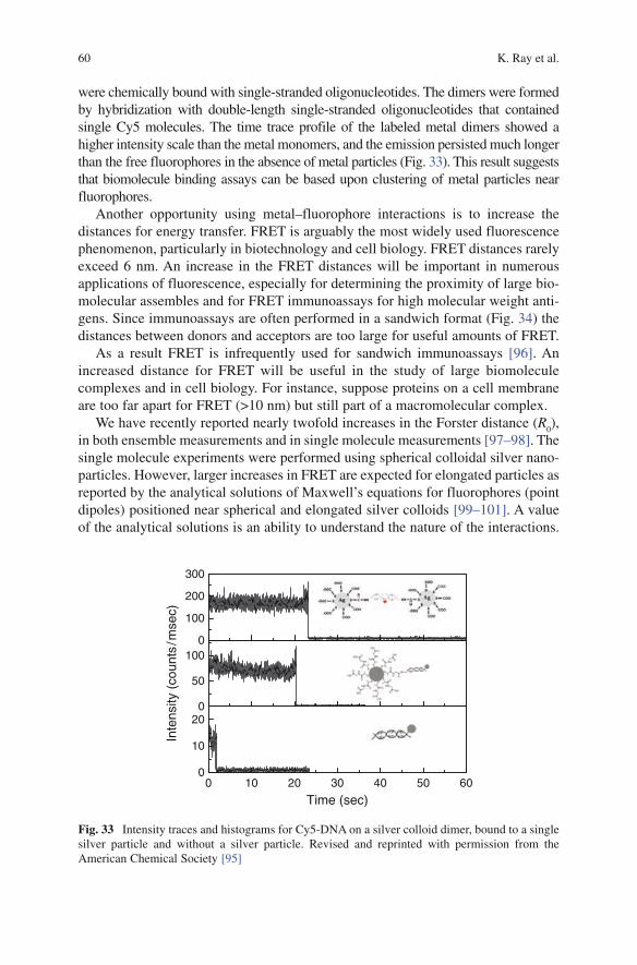
60 K. Ray et al.
were chemically bound with single-stranded oligonucleotides. The dimers were formed by hybridization with double-length single-stranded oligonucleotides that contained single Cy5 molecules. The time trace profile of the labeled metal dimers showed a higher intensity scale than the metal monomers, and the emission persisted much longer than the free fluorophores in the absence of metal particles (Fig. 33). This result suggests that biomolecule binding assays can be based upon clustering of metal particles near fluorophores.
Another opportunity using metal–fluorophore interactions is to increase the distances for energy transfer. FRET is arguably the most widely used fluorescence phenomenon, particularly in biotechnology and cell biology. FRET distances rarely exceed 6 nm. An increase in the FRET distances will be important in numerous applications of fluorescence, especially for determining the proximity of large bio-molecular assembles and for FRET immunoassays for high molecular weight anti-gens. Since immunoassays are often performed in a sandwich format (Fig. 34) the distances between donors and acceptors are too large for useful amounts of FRET.
As a result FRET is infrequently used for sandwich immunoassays [96]. An increased distance for FRET will be useful in the study of large biomolecule complexes and in cell biology. For instance, suppose proteins on a cell membrane are too far apart for FRET (>10 nm) but still part of a macromolecular complex.
We have recently reported nearly twofold increases in the Forster distance (R0),
in both ensemble measurements and in single molecule measurements [97–98]. The single molecule experiments were performed using spherical colloidal silver nano-particles. However, larger increases in FRET are expected for elongated particles as reported by the analytical solutions of Maxwell’s equations for fluorophores (point dipoles) positioned near spherical and elongated silver colloids [99–101]. A value of the analytical solutions is an ability to understand the nature of the interactions.
0 10 20 30 40 50 600
10
200
50
1000
100
200
300
Time (sec)
Inte
nsity
(co
unts
/mse
c)
Fig. 33 Intensity traces and histograms for Cy5-DNA on a silver colloid dimer, bound to a single silver particle and without a silver particle. Revised and reprinted with permission from the American Chemical Society [95]

Plasmon-Controlled Fluorescence Towards High-Sensitivity Optical Sensing 61
Fig. 34 Schematic of energy transfer in a sandwich assay with a change in R0. For this D–A pair
the transfer efficiency is close to 50% for the metal-enhanced R0 = 12 nm and only 1.5% for R
0 = 6
nm without a metal particle
For instance, for metal-enhanced FRET, the effect was seen as a modification of the dipole–dipole interactions between the donor and acceptor. This interaction can result in increased or decreased rates of energy transfer, depending on the size and shape of the particles, the position and distance of the fluorophores from the sur-face, and the orientation of the dipoles relative to the metal surface. The importance of a larger effective Forster distance for immunoassays can be perceived from a specific example. For example, we use a sandwich assay with two IgG molecules and a relatively small antigen like the cardiac marker myoglobin with a molecular weight of 25,000 [102–104] as shown schematically in Fig. 33. If the donor D and acceptor A are located near the center of the IgG molecules they will be about 12 nm apart (Fig. 34). The value of typical Forster distances R
0 is rarely higher than 6
nm. As a result the transfer efficiency will be about 0.015, which is essentially undetectable. Now in the presence of a metal particle if the Forster distance could be increased by twofold, the transfer efficiency increases to 50% and is easily detectable. This example suggests that metal-enhanced FRET can be used to develop FRET immunoassays of large molecular weight antigens.
Single molecule FRET experiments can be used to determine the transfer efficiency of donor–acceptor pairs and the amount of FRET near metal particles [105–106]. We

62 K. Ray et al.
have recently reported a systematic study on the effects of metal particle size, spacer distance between the donor and acceptor, and linker length of the donor–acceptor pair from the metal particle on metal-enhanced FRET. We prepared a donor and acceptor-labeled oligomer which contained a central amino group for binding to the colloid. The length of the oligomers was chosen so there was less than 10% transfer in the absence of the particle (Fig. 35). The transfer efficiency increased dramatically upon binding to the 15 nm colloid, and increased more with increasing particle size. The increase in transfer efficiency is consistent with a 1.7-fold increase in the Forster distance. Assuming the R
0
value in the absence of metal is 6 nm, the effective R0 on the 80 nm particle is 10.2 nm,
which is possibly one of the highest R0 values which have been observed.
To date we have only investigated the effects of spherical particles on FRET. As mentioned earlier, the analytical theory suggests much higher rates of energy transfer when the donor—acceptor pairs are close to elongated particles [99–101]. Such long-range energy transfer may find uses in cell biology. It is known that cellular function can be affected by protein association in the external cell membrane, such as the receptors for epidermal growth factor (EGF). Suppose the EGF receptors are labeled with donors and acceptors, by using either labeled EGF or labeled antibodies to the receptor. Upon receptor association there will be minimal FRET because of the large size of the proteins. Now suppose one of the labeled proteins is bound to an ellipsoi-dal silver colloid about 100 nm long. Then it is possible that the colloid will facilitate FRET over this distance and detect receptor association. It may not be possible to measure the exact donor-to-acceptor distance using metal particles, but it may be pos-sible to detect proximity over distances ranging from 10 to 100 nm. At present it is difficult to measure distances in this range. Electron microscopy requires fixed samples and the resolution of optical microscopy is limited to about 300 nm. Metal-enhanced FRET may allow measurement over this range of distances.
Fig. 35 Respective intensity-time trajectories of a free donor–acceptor pair as observed in the (a) donor channel or (b) the acceptor channel and a donor–acceptor pair bound to a silver particle (c) donor channel and (d) acceptor channel
c
d
Inte
nsity
(co
unts
/ms)
0 1 2 3 4 5
0
200
0 10 µm
0
200
0 10 µm
a
b
0
200
0 10 µm
0
200
0 10 µm
0
200
0 10 µm
0
200
0 10 µm
0
200
0 10 µm0
200
0 10 µm0 10 µm
0
200
0 10 µm0
200
0
200
0 10 µm0 10 µm
Inte
nsity
(co
unt/
ms)
0 5 10 15 200
30
60
90
0
30
60
90
0
200
0 10 µm
0
200
0 10 µm
Time (sec)
0
200
0 10 µm
0
200
0 10 µm
0
200
0 10 µm
0
200
0 10 µm
0
200
0 10 µm
0
200
0 10 µm
0
10
20
30
400
15
30
45
0
200
0 10 µm0
200
0 10 µm0 10 µm
0
200
0 10 µm0
200
0
200
0 10 µm0 10 µm
Time (sec)

Plasmon-Controlled Fluorescence Towards High-Sensitivity Optical Sensing 63
11 Applications of Plasmon-Controlled Fluorescence
In the previous sections we described two types of metallic structures, metal parti-cles for MEF and continuous thin metal films for SPCE. Metal particles and sur-faces represent only a small fraction of the types of metallic structures which can be used to modify fluorescence. Many additional possibilities are available using metallic nanostructures with defined features. The underlying concept is to design the structure to provide wavevectors matching for the desired excitation and emis-sion wavelengths. Perhaps the simplest example of such a structure is a metallic grating. By using a grating structure we can obtain the desired separation by con-trolling the dimensions of the grating.
The use of gratings for PCF can go beyond wavelength resolution. Metal grat-ings are being used to increase the light output of LEDs [107–108]. If the grating is two dimensional then the emission tends to beam away normal to the surface, with some angular separation of wavelengths. Additionally, gratings have been shown to be effective substrates for metal-enhanced fluorescence [109–110]. The enhancements depend on the wavelength of the fluorophore and the period of the grating. It seems likely that one and two-dimensional gratings will soon find use in surface-bound fluorescence assays. The sensitivities can be increased by a combi-nation of MEF due to the patterned structure and by directing more of the emission towards the detector.
Novel devices for fluorescence can be designed using the unique transmission properties of nanohole arrays. One example is shown in Fig. 36 which consists of two nanohole arrays with different spacing between the nanoholes. One array can be designed to transmit shorter wavelength green light for excitation, and the second array can be designed to transmit the longer wavelength red emission. At present such a device may seem too expensive given the high cost of nanofabrication. However, there is rapid progress in high-throughput methods for nanofabrication. One exam-ple is micro-contact printing (MCP). This method depends on nanofabrication of a
Fig. 36 Possible configuration for a sensor based on nanohole arrays
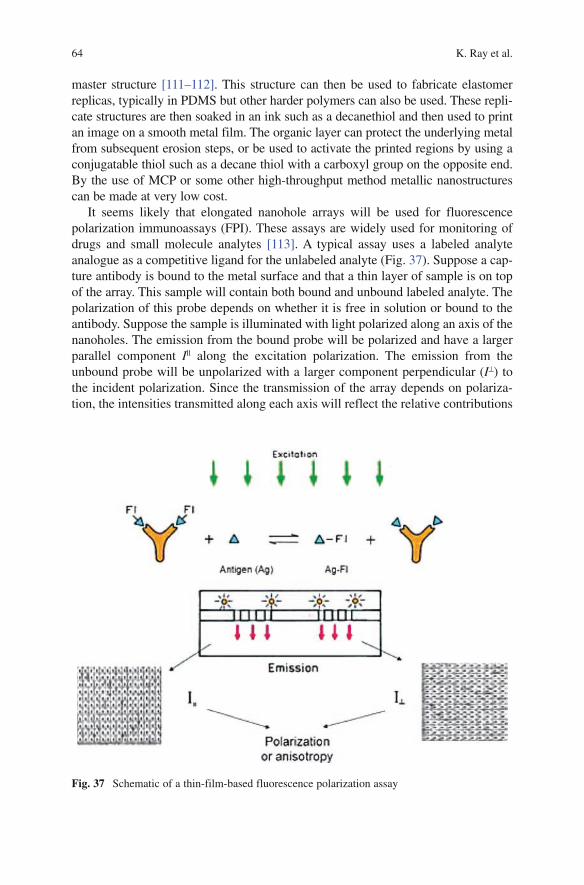
64 K. Ray et al.
master structure [111–112]. This structure can then be used to fabricate elastomer replicas, typically in PDMS but other harder polymers can also be used. These repli-cate structures are then soaked in an ink such as a decanethiol and then used to print an image on a smooth metal film. The organic layer can protect the underlying metal from subsequent erosion steps, or be used to activate the printed regions by using a conjugatable thiol such as a decane thiol with a carboxyl group on the opposite end. By the use of MCP or some other high-throughput method metallic nanostructures can be made at very low cost.
It seems likely that elongated nanohole arrays will be used for fluorescence polarization immunoassays (FPI). These assays are widely used for monitoring of drugs and small molecule analytes [113]. A typical assay uses a labeled analyte analogue as a competitive ligand for the unlabeled analyte (Fig. 37). Suppose a cap-ture antibody is bound to the metal surface and that a thin layer of sample is on top of the array. This sample will contain both bound and unbound labeled analyte. The polarization of this probe depends on whether it is free in solution or bound to the antibody. Suppose the sample is illuminated with light polarized along an axis of the nanoholes. The emission from the bound probe will be polarized and have a larger parallel component Ill along the excitation polarization. The emission from the unbound probe will be unpolarized with a larger component perpendicular (I⊥) to the incident polarization. Since the transmission of the array depends on polariza-tion, the intensities transmitted along each axis will reflect the relative contributions
Fig. 37 Schematic of a thin-film-based fluorescence polarization assay

Plasmon-Controlled Fluorescence Towards High-Sensitivity Optical Sensing 65
of the free and bound probes and the FPI instrument can consist of an elongated nanohole array. Careful design of the nanostructure geometry will be needed to obtain the needed selectivity to each polarized component of the emission [114–115].
12 Use of Metallic Nanostructures for Detection Beyond the Diffraction Limit
In classical far-field optics the spatial resolution is dictated by the spot size of the incident beam (i.e., about 300 nm across a diffraction limited spot) and about 2,000 nm along the optical axis, for a volume of about 1 fL. In order to observe single molecules their emission must be detectable above the Raman scatter and background emission from this volume. As a result single fluorophores can be observed only if these have high quantum yields and are contained in samples with low background emission. Conversely, if smaller volumes can be observed then it may become practical to detect single fluorophores with lower quantum yield fluorophores or detection of single molecules in samples like serum or blood with high background emission. Metallic nanostructures make it possible in some ways to reduce the observed volumes and with a spatial resolution that is well beyond the diffraction limit of the light [116]. One approach is to use the increased fields between pairs of particles. There are many published calculations of the fields between particle dimers [117–118]. However, these calculations do not directly reveal how these fields can be used to obtain sub-wavelength observation volumes. While the fields may be localized it is still necessary to illuminate the structure and the size of the incident beam is still limited by diffraction.
Figure 38 shows the simulated image of local fields induced between two nano-triangles due to the incident plane-wave illumination. The degree of locali-zation is very strong for a pair of triangles. Interestingly, we calculated that even if the entire nanotriangle area were coated with fluorophores, about 25% of the emission would come from the 16 × 16-nm gap region occupying less than 1% of the area. The field calculation suggests that if the triangle pair is uniformly coated with fluorophores a large fraction of the total emission will come from those fluorophores between the tips of the triangle. These calculations suggest that particle clusters can be used to obtain reduced volumes with typical macroscopic optics used to illuminate particle clusters.
Another approach to obtain small volumes is to use the enhanced transmission through nanoholes. When nanoholes in metal films are illuminated there is typi-cally an enhanced field in the nanohole or above the nanohole. This geometry may be preferred because the metal film is expected to block all the light so that the excitation field only exists in or above the nanohole. However, it is known that light incident on a single nanohole can induce plasmons on the distal side of the film [119] so that completely localized excitation may not always occur. Nonetheless, nanoholes are promising structures for obtaining small volumes.
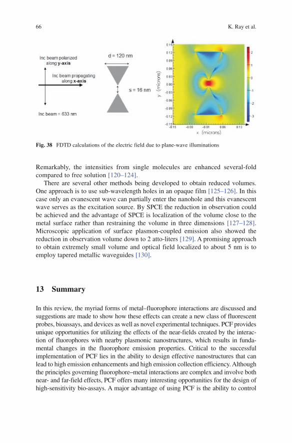
66 K. Ray et al.
Remarkably, the intensities from single molecules are enhanced several-fold compared to free solution [120–124].
There are several other methods being developed to obtain reduced volumes. One approach is to use sub-wavelength holes in an opaque film [125–126]. In this case only an evanescent wave can partially enter the nanohole and this evanescent wave serves as the excitation source. By SPCE the reduction in observation could be achieved and the advantage of SPCE is localization of the volume close to the metal surface rather than restraining the volume in three dimensions [127–128]. Microscopic application of surface plasmon-coupled emission also showed the reduction in observation volume down to 2 atto-liters [129]. A promising approach to obtain extremely small volume and optical field localized to about 5 nm is to employ tapered metallic waveguides [130].
13 Summary
In this review, the myriad forms of metal–fluorophore interactions are discussed and suggestions are made to show how these effects can create a new class of fluorescent probes, bioassays, and devices as well as novel experimental techniques. PCF provides unique opportunities for utilizing the effects of the near-fields created by the interac-tion of fluorophores with nearby plasmonic nanostructures, which results in funda-mental changes in the fluorophore emission properties. Critical to the successful implementation of PCF lies in the ability to design effective nanostructures that can lead to high emission enhancements and high emission collection efficiency. Although the principles governing fluorophore–metal interactions are complex and involve both near- and far-field effects, PCF offers many interesting opportunities for the design of high-sensitivity bio-assays. A major advantage of using PCF is the ability to control
Fig. 38 FDTD calculations of the electric field due to plane-wave illuminations
Plasmon-Controlled Fluorescence Towards High-Sensitivity Optical Sensing 67
the excitation and emission processes of fluorescent molecules, and this complements existing technology that is used for designing and synthesizing new fluorescent probes. Additionally, PCF allows the spatial distribution of the emission to be controlled with nearby metallic nanostructures instead of the usual macroscopic optics.
Acknowledgments This work was supported by National Institutes of Health (Grant nos. HG002655, EB006521, and EB00682).
References
1. Strickler SJ, Berg RA (1962) Relationship between absorption intensity and fluorescence lifetimes of molecules. J Chem Phys 37:814–822
2. Yguerabide J, Yguerabide EE (1998) Light-scattering submicroscopic particles as highly fluo-rescent analogs and their use as tracer labels in clinical and biological applications: I. Theory. Anal Biochem 262:137–156
3. Yguerabide J, Yguerabide EE (1998) Light-scattering submicroscopic particles as highly fluo-rescent analogs and their use as tracer labels in clinical and biological applications: II. Experimental characterization. Anal Biochem 262:157–176
4. Schultz S, Smith SR, Mock JJ, Schulz DA (2000) Single target molecule detection with nonbleaching multicolor optical immunolabels. Proc Natl Acad Sci U S A 97:996–1001
5. Sokolov K, Follen M, Aaron J, Pavlova I, Malpica A, Lotan R, Richards-Kortum R (2003) Real-time vital optical imaging of precancer using anti-epidermal growth factor receptor antibodies conjugated to gold nanoparticles. Cancer Res 63:199–2004
6. Chowdhury MH, Gray SK, Pond J, Geddes CD, Aslan K, Lakowicz JR (2007) Computational study of fluorescence scattering by silver nanoparticles. J Opt Soc Am B 24:2259–2267
7. Mayergoyz ID, Zhang Z, Miano G (2007) Analysis of dynamics of excitation and dephasing of plasmon resonance modes in nanoparticles. Phys Rev Lett 98:147401–1/4
8. Pelton M, Liu M, Park S, Scherer NF, Guyor-Sionnest P (2006) Ultrafast resonant optical sensing from single gold nanorods: large nonlinearities and plasmon saturation. Phys Rev B 73:155419–1/6
9. Lakowicz JR (2001) Radiative decay engineering: biophysical and biomedical applications. Anal Biochem 298:1–24
10. Lakowicz JR, Shen Y, D’Auria S, Malicka J, Fang J, Gryczynski Z, Gryczynski I (2002) Radiative decay engineering. 2. Effects of silver island films on fluorescence intensity, life-times, and resonance energy transfer. Anal Biochem 301:261–277
11. Lakowicz JR (2004) Radiative decay engineering 3: surface plasmon coupled emission. Anal Biochem 324:153–169
12. Gryczynski I, Malicka J, Gryczynski Z, Lakowicz JR (2004) Radiative decay engineering 4: experimental studies of surface plasmon coupled emission. Anal Biochem 324:170–182
13. Sokolov K, Chumanov G, Cotton TM (1998) Enhancement of molecular fluorescence near the surface of colloidal metal films. Anal Chem 70:3898–3905
14. Amos RM, Barnes WL (1997) Modification of the spontaneous emission rate of Eu3+ ions close to a thin metal mirror. Phys Rev B 55(11):7249–7254
15. Barnes WL (1998) Fluorescence near interfaces: the role of photonic mode density. J Mod Opt 45(4):661–699
16. Weitz DA, Garoff S, Hanson CD, Gramila TJ (1982) Fluorescent lifetimes of molecules on silver-island films. Opt Lett 7(2):89–91
17. Aussenegg FR, Leitner A, Lippitsch ME, Reinisch H, Reigler M (1987) Novel aspects of fluo-rescence lifetime for molecules positioned close to metal surfaces. Surf Sci 139:935–945
68 K. Ray et al.
18. Leitner A, Lippitsch ME, Draxler S, Riegler M, Aussenegg FR (1985) Fluorescence properties of dyes absorbed to silver islands, investigated by picosecond techniques. Appl Phys B 36:105–109
19. Sabanayagam C, Lakowicz JR (2007) Increasing the sensitivity of DNA microarrays by metal-enhanced fluorescence using surface-bound silver nanoparticles. Nucleic Acids Res 35:e13
20. Gu T, Whitesell JK, Fox MA (2003) Energy transfer from a surface bound arene to the gold core in fluorenyl-alkane-1-thiolate monolayer-protected gold clusters. Chem Mater 15:1358–1366
21. Gueroui Z, Liebchaber A (2004) Single-molecule measurements of gold quenched quantum dots. Phys Rev Lett 93:166108–166114
22. Ipe BI, Thomas KG (2002) Photoinduced charge separation in a fluorophore-Gold assembly. J Phys Chem B 106:18–21
23. Aguila A, Murray RW (2000) Monolayer-protected clusters with fluorescent dansyl ligands. Langmuir 16:5949–5954
24. Yun CS, Javier A, Jennings T, Fisher M, Hira S, Peterson S, Hopkins B, Reich NO, Strouse GF (2002) Nanometal surface energy transfer in optical rulers, breaking the FRET barrier. J Am Chem Soc 127:3115–3119
25. Fan C, Wang S, Hong JW, Bazan GC, Plaxco KW, Heeger AJ (2003) Beyond superquenching: hyper-efficient energy transfer from conjugated polymers to gold-nanoparticles. Proc Natl Acad Sci U S A 100:6297–6301
26. Zhang J, Lakowicz JR (2007) Metal-enhanced fluorescence of an organic fluorophore using gold particles. Opt Exp 15(5):2598–2606
27. Garoff S, Weitz DA, Alvarez MS, Gersten JI (1984) Electrodynamics at rough metal surfaces: photochemistry and luminescence of adsorbance near metal-island films. J Chem Phys 81(11):5189–5200
28. Ray K, Chowdhury M, Lakowicz JR (2007) Aluminum nano-structured film as a substrate for enhanced fluorescence in the ultraviolet – blue spectral region. Anal Chem 79:6480–6487
29. Ray K, Badugu R, Lakowicz JR (2006) Metal-enhanced fluorescence from CdTe nanocrys-tals: a single-molecule fluorescence study. J Am Chem Soc 128:8998–8999
30. Okamoto K, Vyawahare S, Scherer A (2006) Surface-plasmon enhanced bright emission from CdSe quantum-dot nanocrystals. J Opt Soc Am B 23:1674–1678
31. Shimizu KT, Woo WK, Fisher BR, Eisler HJ, Bawendi MG (2002) Surface-enhanced emis-sion from single semiconductor nanocrystals. Phys Rev Lett 89:117401–1/4
32. Chowdhury MH, Ray K, Aslan K, Lakowicz JR, Geddes CD (2007) Enhanced fluorescence of phycobiliproteins from plasmonic nanostructures. J Phys Chem C 111:18856–18863
33. Lakowicz JR, Maliwal BP, Malicka J, Gryczynski Z, Gryzynski I (2002) Effects of silver island films on the luminescent intensity and decay times of lanthanide chelates. J Fluoresc 12(3/4):431–437
34. Wu M, Lakowicz JR, Geddes CD (2005) Enhanced lanthanide luminescence using silver nanostructures: opportunities for a new class of probes with exceptional spectra characteris-tics. J Fluoresc 15:53–59
35. Daniel E, Weber G (1966) Cooperative effects in binding by bovine serum albumin, I: the binding of 1-anilino-8-naphthalenesulfonate. Fluorimetric titrations. Coop Effects Binding Albumin 5:1893–1900
36. Slavik J (1982) Anilinonaphthalene sulfonate as a probe of membrane composition and func-tion. Biochim Biophys Acta 694:1–25
37. Benson SC, Zeng Z, Glazer AN (1995) Fluorescence energy-transfer cyanine heterodimers with high affinity for double-stranded DNA. Anal Biochem 231:247–255
38. Haq I, Ladbury JE, Chowdhry BZ, Jenkins TC, Chaires JB (1997) Specific binding of Hoechst 33258 to the D(CGCAAATTTGCG)
2 duplex: calorimetric and spectroscopic studies. J Mol
Biol 271:244–257 39. Glazer AN, Peck K, Matheis RA (1990) A stable double-stranded DNA ethidium homodimer
complex: application to picogram fluorescence detection of DNA in agarose gels. Proc Natl Acad Sci U S A 87:3851–3855
Plasmon-Controlled Fluorescence Towards High-Sensitivity Optical Sensing 69
40. Rye HS, Yue S, Wemmer DE, Quesada MA, Haugland RP, Mathies RA, Glazer AN (1992) Stable fluorescent complexes of double-stranded DNA with bis-intercalating asymmetric cyanine dyes: properties and applications. Nucleic Acids Res 20(11:):2803–2812
41. Malicka J, Gryczynski I, Lakowicz JR (2003) DNA hybridization assays using metal-enhanced fluorescence. Biochem Biophys Res Commun 306:213–218
42. Enderlein J (2002) Spectral properties of a fluorescing molecule within a spherical metallic cavity. Phys Chem Chem Phys 4:2780–2786
43. Enderlien J (2002) Theoretical study of single molecule fluorescence in a metallic nanocavity. Appl Phys Lett 80:315–317
44. Zhang J, Gryczynski I, Gryczynski Z, Lakowicz JR (2006) Dye-labeled silver nanoshell – bright particle. J Phys Chem B 110:8986–8991
45. Aslan K, Lakowicz JR, Geddes CG (2007) Metal enhanced fluorescence solution-based sens-ing platform 2: fluorescent core-shell Ag@SiO
2 nanoballs. J Fluoresc 17:127–131
46. Aslan K, Wu M, Lakowicz JR, Geddes CG (2007) Fluorescent core – shell Ag@SiO2 nano-
composites for meta-enhanced fluorescence and single nanoparticle sensing platforms. J Am Chem Soc 129:1524–1425
47. Hemmila IA (1991) Applications of fluorescence in immunoassays. John Wiley & Sons, New York, 360 p
48. Soini E, Hemmila IA, Dahlen D (1995) Time-resolved fluorescence in biospecific assays (review). Pharmacol Ther 66:207–235
49. Yan Y, Marriott G (2003) Analysis of protein interactions using fluorescence technologies. Curr Opin Chem Biol 7:635–640
50. Goldsby RA, Kindt TJ, Osborne BA, Kuby J (2003) Enzyme-linked immunosorbent assay. In: Immunology, 5th edn. Freeman, New York, pp. 148–160
51. Szmacinski H, Smith D, Hanson MA, Kostov Y, Lakowicz JR, Rao G (2008) A novel method for monitoring monoclonal antibody production during cell culture. Biotechnol Bioengin 100:448–457
52. Findlay JWA, Smith WC, Lee JW, Nordblom GD, Das I, DeSilva BS, Khan MN, Bowsher RR (2000) Validation of immunoassays for bioanalysis: a pharmaceutical industry perspective. J Pharm Biomed Anal 21:1249–1273
53. Szmacinski H, Lakowicz JR (1999) Measurement of the intensity of long lifetime lumino-phores in the presence of background signals using phase-modulation fluorometry. Appl Spectrosc 53:1490–1494
54. Lakowicz JR (2006) Principles of fluorescence spectroscopy, 3rd edn. Springer Science, New York, pp. 158–204
55. Harms P, Sipior J, Ram N, Carter GM, Rao G (1999) Low cost phase-modulation measure-ments of nanosecond fluorescence lifetimes using a lock-in amplifier. Rev Sci Instrum 70(2):1535–1539
56. Calander N (2005) Surface plasmon-coupled emission and Fabry-Perot resonance in the sam-ple layer: a theoretical approach. J Phys Chem B 109:13957–13956
57. Calander N (2004) Theory and simulation of surface plasmon-coupled directional emission from fluorophores at planar structures. Anal Chem 76:2168–2173
58. Salamon Z, Macleod HA, Tollin G (1997) Surface plasmon resonance spectroscopy as a tool for investigating the biochemical and biophysical properties of membrane protein systems. I: Theoretical principles. Biochim Biophy Acta 1331:117–129
59. Melendez J, Carr R, Bartholomew DU, Kukanskis K, Elkind J, Yee S, Furlong C, Woodbury R (1996) A commercial solution for surface plasmon sensing. Sens Actuators B 35–36:212–216
60. Liedberg B, Lundstrom I (1993) Principles of biosensing with an extended coupling matrix and surface plasmon resonance. Sens Actuators B 11:63–72
61. Cooper MA (2002) Optical biosensors in drug discovery. Nat Rev 1:515–528 62. Wegner GJ, Lee HJ, Corn RM (2002) Characterization and optimization of peptide arrays for
the study of epitope-antibody interactions using surface plasmon resonance imaging. Anal Chem 74:5161–5168
70 K. Ray et al.
63. Natan MJ, Lyon LA (2002) Surface plasmon resonance biosensing with colloidal Au amplifi-cation. In: Feldheim DL, Foss CA (eds.) Metal nanoparticles: synthesis, characterization, and applications. Marcel Dekker, New York, pp. 183–205
64. Raether H (1977) Surface plasmon oscillations and their applications. Physics of thin films. In: Hass G, Francombe MH, Hoffman RW (eds.) Advances in research and development. Academic Press, New York, Vol. 9, pp. 145–261
65. Yih J, Chien F, Lin C, Yau H, Chen S (2005) Angular interrogation attenuated total reflection metrology system for plasmonic structures. Appl Opt 44:6155–6162
66. Skivesen N, Horvath R, Pederson HC (2005) Optimization of metal-clad waveguide sensors. Sens Actua B 106:668–676
67. Barnes WL (1998) Fluorescence near interfaces: the role of photonic mode density. J Mod Opt 45(4):661–699
68. Drexhage KH (1970) Influence of a dielectric interface on fluorescence decay time. J Luminescence 2:693–701
69. Benner RE, Dornhaus R, Chang RK (1979) Angular emission profiles of dye molecules excited by surface plasmon waves at a metal surface. Opt Commun 30(2):145–149
70. Weber WH, Eagen CF (1979) Energy transfer from an excited dye molecule to the surface plasmons of an adjacent metal. Opt Lett 4(8):236–238
71. Isfort G, Schierbaum K, Zerulla D (2006) Causality of surface plasmon polariton emission processes. Phys Rev B 73:033408–1/4
72. Chowdhury MH, Malyn SN, Aslan K, Lakowicz JR, Geddes JR (2006) Multicolor directional surface plasmon coupled chemiluminescence. J Phys Chem B 110:22644–22651
73. Kostov Y, Smith DS, Tolosa L, Rao G, Gryczynski I, Gryczynski Z, Malicka J, Lakowicz JR (2005) Directional surface plasmon-coupled emission from a 3 nm green fluorescent protein monolayer. Biotechnol Prog 21:1731–1735
74. Neal TD, Okamoto K, Scherer A (2005) Surface plasmon enhanced emission from dye doped polymer layers. Opt Exp 13(14):5522–5527
75. Ray K, Badugu R, Lakowicz JR (2007) Sulforhodamine adsorbed Langmuir–Blodgett layers on silver island films: effect of probe distance on the metal-enhanced fluorescence. J Phys Chem C 111:7091–7097
76. Ray K, Badugu R, Lakowicz JR (2007) Polyelectrolyte layer-by-layer assembly to control the distance between fluorophores and plasmonic nanostructures. Chem Mater 111:7091–7097
77. Ray K, Szmacinski H, Enderlein J, Lakowicz JR (2007) Distance dependence of surface plasmon-coupled emission observed using Langmuir—Blodgett films. Appl Phys Lett 90:251116–1/3
78. Chowdhury MH, Ray K, Geddes CD Lakowicz JR (2008) Use of silver nanoparticles to enhance surface plasmon-coupled emission (SPCE). Chem Phys Lett 452:162–167
79. Matveeva EG, Gryczynski Z, Malicka J, Lukomska J, Makowiec S, Berndt KW, Lakowicz JR, Gryczynski I (2005) Directional surface plasmon-coupled emission: application for an immunoassay in whole blood. Anal Biochem 344:161–167
80. Matveeva EG, Gryczynski I, Barnett A, Leonenko Z, Lakowicz JR, Gryczynski Z (2007) Metal particle-enhanced fluorescent immunoassays on metal mirrors. Anal Biochem 363:239–245
81. Gryczynski I, Malicka J, Nowaczky K., Gryczynski Z, Lakowicz JR (2006) Waveguide-modulated surface plasmon-coupled emission of Nile blue in poly(vinyl alcohol) thin films. Thin Solid Films 510:15–20
82. Gryczynski I, Malicka J, Nowaczyk K, Gryczynski Z, Lakowicz JR (2004) Effects of sample thickness on the optical properties of surface plasmon-coupled emission. J Phys Chem B 108:12073–12083
83. Stefani FD, Vasilev K, Bocchio N, Stoyanova N, Kreiter M (2005) Surface-plasmon-mediated single molecule fluorescence through a thin metallic film. Phys Rev Lett 94:023005–1/4
84. Vasilev K, Knoll W, Kreiter M (2004) Fluorescence intensities of chromophores in front of a thin metal film. J Chem Phys 120(7):3439–3445

Plasmon-Controlled Fluorescence Towards High-Sensitivity Optical Sensing 71
85. Fu Y, Lakowicz JR (2006) Enhanced fluorescence of Cy5-labeled DNA tethered to silver island films: fluorescence images and time-resolved studies using single-molecule spectros-copy. Anal Chem 78:6238–6245
86. Fu Y, Lakowicz JR (2006) Enhanced fluorescence of Cy5-labeled oligonucleotides near sil-ver island films: a distance effect study using single molecule spectroscopy. J Phys Chem B 110:22557–22562
87. Moerner WE (1997) Those blinking single molecules. Science 277:1059–1060 88. Dickson R, Cubitt A, Tsien R, Moerner WE (1997) On/off blinking and switching behaviour
of single molecules of green fluorescent protein. Nature 388:355–358 89. Rasnik I, McKinney SA, Ha T (2006) Nonblinking and long lasting single molecule fluores-
cence imaging. Nat Methods 3:891–893 90. Zhang J, Fu Y, Chowdhury MH, Lakowicz JR (2008) Single molecule studies on fluores-
cently labeled particles: effects of particle size. J Phys Chem C 112:18–26 91. Ford GW, Weber WH (1984) Electromagnetic interactions of molecules with metal surfaces.
Phys Rep 113(4):195–287 92. Gersten J, Nitzan A (1981) Spectroscopic properties of molecules interacting with small
dielectric particles. J Chem Phys 75(3):1139–1152 93. Kneipp K, Kneipp H, Deinum G, Itzkan I, Dasari RR, Feld MS (1998) Single-molecule
detection of a cyanine dye in silver colloidal solution using near-infrared surface-enhanced Raman scattering. Appl Spectrosc 52(2):175–178
94. Kneipp K, Wang Y, Kneipp H, Perelman L, Itzkan I, Dasari RR, Feld MS (1997) Single molecule detection using surface-enhanced Raman scattering (SERS). Phys Rev Lett 78(9):1667–1670
95. Zhang J, Fu Y, Chowdhury MH, Lakowicz JR (2007) Metal-enhanced single-molecule fluo-rescence on silver particle monomer and dimer: coupling effect between metal particles. Nano Lett 7:2101–2107
96. Ullman EF, Schwarzberg M, Rubenstein KE (1976) Fluorescent excitation transfer immu-noassay: a general method for determination of antigens. J Biol Chem 251(14):4172–4178
97. Malicka J, Gryczynski I, Kusba J, Lakowicz JR (2003) Effects of metallic silver island films on resonance energy transfer between N,N′-(dipropyl)-tetramethyl-indocarbocyanine (Cy3)- and N,N′(dipropyl)-tetramethyl-indodicarbocyanine (cy5)-labeled DNA. Biopolymers 70:595–603
98. Zhang J, Fu Y, Lakowicz JR (2007) Enhanced Forster resonance energy transfer (FRET) on a single metal particle. J Phys Chem C 111:50–56
99. Gersten JI, Nitzan A (1983) Accelerated energy transfer between molecules near a solid particle. Chem Phys Lett 104:31–37
100. Hua XM, Gersten JI, Nitzan A (1985) Theory of energy transfer between molecules near solid state particles. J Chem Phys 83:3650–3654
101. Gersten JI (2005) Theory of fluorophore-metallic surface interactions. In: Topics in fluores-cence spectroscopy. Radiative decay engineering, Vol. 8. Springer, New York, p. 197
102. Christenson RH, Azzazy HME (1999) Evidence based approach to practice guides and deci-sion thresholds for cardiac markers. Scand J Clin Lab Invest 59(Suppl 230):90–102
103. Newby LK, Storrow AB, Gibler WB, et al. (2001) Bedside multimarker testing for risk stratification in chest pain units: the chest pain evaluation by creatine kinase-MB, myoglobin, and troponin I(CHECKMATE) study. Circulation 103:1832–1837
104. Christenson RH, Azzazy HME (1998) Biochemical markers of the acute coronary syn-dromes. Clin Chem 44:1855–1864
105. Zhang Z, Fu Y, Lakowicz JR (2007) Enhanced Forster resonance energy transfer (FRET) on a single metal particle. J Phys Chem C 111:50–56
106. Zhang Z, Fu Y, Lakowicz JR (2007) Enhanced Forster resonance energy transfer (FRET) on single metal particle 2: dependence on donor-acceptor separation distance, particle size, and distance from metal surface. J Phys Chem C 111:11784–11792
107. Gifford DK, Hall DG (2002) Emission through one of two metal electrodes of an organic light-emitting diode via surface-plasmon cross coupling. Appl Phys Lett 81(23):4315–4317
72 K. Ray et al.
108. Feng J, Okamoto T, Kawata S (2005) Highly directional emission via coupled surface-plasmon tunneling from electroluminescence in organic light-emitting devices. Appl Phys Lett 87:241109–1/3
109. Matthews DR, Summers HD, Njoh k, Chappell S, Errington R, Smith P, Pope I, Barber P, Vojnovic B, Ameer-Beg S (2007) A fluorescence biochip with a plasmon active surface. Proc SPIE 6450:645006–1/8
110. Hung Y-J, Smolyaninov II, Davis CC (2006) Fluorescence enhancement by surface gratings. Opt Exp 14(22):10825–10830
111. Xia Y, Whitesides GM (1998) Soft lithography. Annu Rev Mater Sci 28:153 112. Milan M, Whitesides GM (1995) Patterning self-assembled monolayers using microcontact
printing: a new technology for biosensors. TIBTECH 13:228–231 113. Dandliker WB, de Saussure VA (1970) Fluorescence polarization in immunochemistry.
Immunochemistry 7:799–828 114. Van der Molen KL, Klein Koerkamp KJ, Enoch S, Segerink FB, van Hulst NF, Kuipers L
(2005) Role of shape and localized resonances in extraordinary transmission through peri-odic arrays of subwavelength holes: experiment and theory. Phys Rev B 72:045421–1/9
115. Elliott J, Smolyaninov II, Zheludev NI, Zayats AV (2004) Polarization control of optical transmission of a periodic array of elliptical nanoholes in a metal film. Opt Lett 29(12):1414–1416
116. Stewart ME, Anderton CR, Thompson LB, Maria J, Gray SK, Rogers JA, Nuzzo RG (2008) Nanostructured plasmonic sensors. Chem Rev 108:494–521
117. Jin EX, Xu X (2006) Enhanced optical near field from a bowtie aperture. Appl Phys Lett 88:143110–1/
118. Wang L, Uppuluri SM, Jin EX, Xu X (2006) Nanolithography using high transmission nano-scale bowtie apertures. Nano Lett 6(3):361–364
119. Yin L, Vlasko-Vlasov VK, Rydh A, Pearson J, Welp U, Chang S-H, Gray SK, Schatz GC, Brown DB, Kimball CW (2004) Surface plasmons at single nanoholes in Au films. Appl Phys Lett 85(3):467–469
120. Popov E, Neviere M, Wenger J, Lenne P-F, Rigneault H, Chaumet P (2006) Field enhance-ment in single subwavelength apertures. J Opt Soc Am A 23(9):2342–2348
121. Kim JH, Moyer PJ (2007) Laser-induced fluorescence within subwavelength metallic arrays of nanoholes indicating minimal dependence on hole periodicity. Appl Phys Lett 90:131111–1/3
122. Wenger J, Lenne P-F, Popov E, Rigneault H (2005) Single molecule fluorescence in rectan-gular nano-apertures. Opt Exp 13(18):7035–7044
123. Rigneault H, Capoulade J, Dintinger J, Wenger J, Bonod N, Popov E, Ebbesen TW, Lenne P-F (2005) Enhancement of single-molecule fluorescence detection in subwavelength aper-tures. Phys Rev Lett 95:117401–1/4
124. Liu Y, Mahdavi F, Blair S (2005) Enhanced fluorescence transduction properties of metallic nanocavity arrays. IEEE J Sel Top Quantum Electronics 11(4):778–784
125. Samiee KT, Moran-Mirabal JM, Cheung YK, Craighead HG (2006) Zero mode waveguides for single-molecule spectroscopy on lipid membranes. Biophys J 90:3288–3299
126. Levene MJ, Korlach J, Turner SW, Foquet M, Craighead HG, Webb WW (2003) Zero-model waveguides for single-molecule analysis at high concentrations. Science 299:682–868
127. Gryczynski Z, Borejdo J, Calander N, Matveeva EG, Gryczynski I (2006) Minimization of detection volume by surface-plasmon coupled emission. Anal Biochem 356:125–131
128. Gryczynski I, Malicka J, Lakowicz JR, Goldys EM, Calander N, Gryczynski Z (2005) Directional two-photon induced surface plasmon-coupled emission. Thin Solid Films 491:173–176
129. Borejdo J, Gryczynski Z, Calander N, Muthu P, Gryczynski I (2006) Application of surface-plasmon coupled emission to study muscles. Biophys J 91:2626–2635
130. Issa NA, Guckenberger R (2007) Optical nanofocusing on tapered metallic waveguides. Plasmonics 2:31–37
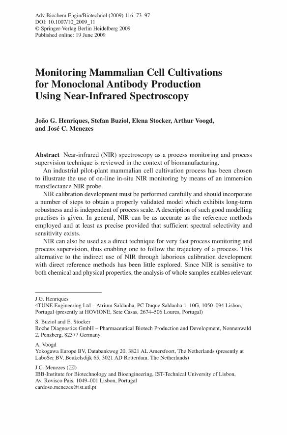
Monitoring Mammalian Cell Cultivations for Monoclonal Antibody Production Using Near-Infrared Spectroscopy
João G. Henriques, Stefan Buziol, Elena Stocker, Arthur Voogd, and José C. Menezes
J.G. Henriques 4TUNE Engineering Ltd – Atrium Saldanha, PC Duque Saldanha 1–10G, 1050–094 Lisbon, Portugal (presently at HOVIONE, Sete Casas, 2674–506 Loures, Portugal)
S. Buziol and E. Stocker Roche Diagnostics GmbH – Pharmaceutical Biotech Production and Development, Nonnenwald 2, Penzberg, 82377 Germany
A. Voogd Yokogawa Europe BV, Databankweg 20, 3821 AL Amersfoort, The Netherlands (presently at LaboSer BV, Beukelsdijk 65, 3021 AD Rotterdam, The Netherlands)
J.C. Menezes () IBB-Institute for Biotechnology and Bioengineering, IST-Technical University of Lisbon, Av. Rovisco Pais, 1049–001 Lisbon, [email protected]
Abstract Near-infrared (NIR) spectroscopy as a process monitoring and process supervision technique is reviewed in the context of biomanufacturing.
An industrial pilot-plant mammalian cell cultivation process has been chosen to illustrate the use of on-line in-situ NIR monitoring by means of an immersion transflectance NIR probe.
NIR calibration development must be performed carefully and should incorporate a number of steps to obtain a properly validated model which exhibits long-term robustness and is independent of process scale. A description of such good modelling practises is given. In general, NIR can be as accurate as the reference methods employed and at least as precise provided that sufficient spectral selectivity and sensitivity exists.
NIR can also be used as a direct technique for very fast process monitoring and process supervision, thus enabling one to follow the trajectory of a process. This alternative to the indirect use of NIR through laborious calibration development with direct reference methods has been little explored. Since NIR is sensitive to both chemical and physical properties, the analysis of whole samples enables relevant
Adv Biochem Engin/Biotechnol (2009) 116: 73–97DOI: 10.1007/10_2009_11© Springer-Verlag Berlin Heidelberg 200Published online: 19 June 2009
9

74 J.G. Henriques et al.
process information to be captured and thus generates better process state estimates than by simply looking at defined process parameters one at a time.
Keywords Process Analytical Technology • Biomanufacturing • Process Spectro scopy • NIR • mammalian cells cultivation
Contents
1 Introduction ................................................................................................................................... 751.1 Process Monitoring ............................................................................................................. 761.2 Process Supervision ............................................................................................................ 761.3 Process Diagnosis and Control ........................................................................................... 771.4 NIR Spectroscopy ............................................................................................................... 771.5 Sampling Interfaces ............................................................................................................ 781.6 NIR in Bioprocess Monitoring ........................................................................................... 791.7 Chemometrics: Multivariate Data Analysis ....................................................................... 80
2 Case Study .................................................................................................................................... 802.1 Development of Models for the Quantitative Determination of Key Analytes .................. 812.2 Sample Selection: Calibration and External Validation ..................................................... 812.3 Internal Validation .............................................................................................................. 832.4 Spectral Pre-Processing ...................................................................................................... 842.5 Variable Selection ............................................................................................................... 852.6 Outlier Detection ................................................................................................................ 862.7 Quantitative Methods ......................................................................................................... 872.8 Process Supervision: Mapping Process Trajectories .......................................................... 912.9 Detection of a Contamination ............................................................................................. 93
3 Conclusions ................................................................................................................................... 94References ........................................................................................................................................... 95
Symbols and Abbreviations
GA Genetic AlgotithmHPLC High performance liquid chromatographyLV Latent variableMab Monoclonal antibodyNIR Near-infraredNIRS NIR SpectroscopyPAT Process analytical technologyPC Principal componentPCA Principal component analysisPLS Partial least-squaresR 2
cv Correlation coefficient for cross-validation predictions
R 2p Correlation coefficient for external validation predictions
RMSECV Root mean square error of cross-validationRMSEP Root mean square error of predictionSEL Standard error of laboratorySG Savitzky–GolaySNV Standard normal variateVIP Variable importance plot
Monitoring Mammalian Cell Cultivations for Monoclonal Antibody Production 75
Glossary
Genetic algorithm Numerical method for feature selection based on the mechanisms of biologic evolution
Loadings Matrix describing how the original variables relate to the new principal components of a PCA
Partial least-squares linear modelling technique used for regression of large sets of collinear variables (X block) with a cor-related response (Y vector)
Principal component analysis Data factorisation methods that creates new orthog-onal variables called principal components as linear combination of the original variables capturing the most possible variance in the original data
Scores Projection of an observation (sample) in the principal component space of a PCA
1 Introduction
A rational description of the metabolic and regulatory networks inside a cell in con-junction with cell morphology issues and population dynamics is not achievable in practice for most commercial bioproducts. The cell largely controls its own processes within the narrow range of extracellular conditions provided through human interven-tion. For most processes pre-established process recipes are used initially to grow biomass and then induce production of the required product. Moreover, bioprocesses are strongly influenced by the quality of inocula and raw-materials used. As such, it is understandable that: (1) the number of parameters measured in a bioprocess are often only some of those related to what can be controlled (e.g. cell density, pH, extracellular concentration of substrates); (2) sampling frequency is very conservative since these parameters are manipulated at a low frequency; (3) process development is time con-suming and complex mainly because a large number of experiments must be carried out to generate enough process knowledge out of the many possible combinations of variables involved (i.e. strain or cell lines used, raw-material conditioning and media formulation, inocula scale-up and fermentation operation). Hence insufficient infor-mation is acquired during a batch to allow the characterization of the bioprocess state at any given cultivation time. Furthermore, any PAT strategy developed for a dynamic process whose trajectory strongly depends on the starting conditions (e.g. inocula qual-ity or previous development steps) must take into account information from previous processing stages if a precise end-point is to be achieved consistently.
One possible and obvious strategy to cope with these difficulties would involve: (1) monitoring intensification (more parameters measured more frequently in all relevant steps); (2) tools to pull together the information of several fermentation batches (building and navigating a design space); and (3) systems engineering tools to analyse several runs of the entire process (thus describing the interactions
76 J.G. Henriques et al.
between process components). We have successfully developed and applied such a strategy to the biomanufacturing of several anti-infectives [1, 2] and we believe that it will be of general value to other bioprocesses including those involving animal cells for the production of Mabs. Once an overall quantitative description of proc-ess is in place, a PAT strategy for closed loop control can be devised based on the elements: monitoring, supervision, diagnosis and control.
1.1 Process Monitoring
Large amounts of highly informative data are of course much easier to obtain with on-line multi-parametric techniques (e.g. in-situ spectroscopy or fermentation off-gas analysis) than with fast at-line mono-parametric techniques. A particular advantage of multi-parametric techniques is that rather than merely monitoring a limited number of parameters they are able to take a sample’s fingerprint and thus capture the combined effects of its chemical and physical attributes. One such technique is NIR Spectroscopy (NIRS) which is capable of accurate bioprocess monitoring in systems as diverse as fungi, bacterial and animal cell fermentations [3]. This is a very versatile technique with a well-established process monitoring track record in several processing industries. A technician proficient in chemometrics and on the other hand familiar with the process to be monitored (e.g. its dynamics and main influencing factors and sources of variability) will be able to establish robust and accurate calibrations valid across different process scales or in similar in nature processing steps [4, 5]. However, an approach that is less commonly used in this area is the use of NIR as a process fingerprinting technique. In this case, advantage is taken of its intrinsic ability to capture a sample’s chemical and physical informa-tion, thus avoiding the need for calibration development and making the most of the availability of on-line in-situ measurements for batch supervision.
1.2 Process Supervision
Process supervision considers several types of variables, i.e. it is multivariate. Process supervision is not only monitoring in perspective (i.e. the incoming monitored data point for a variable is plotted and compared to that variable’s history along the batch); it attains a higher level by comparing the running batch against previous batches (e.g. charting the running batch trajectory over the nominal batch trajectory). While taking a batch perspective by analysing several historical batches in a consolidated manner, PAT as a process supervision tool has significant potential in process analysis and understanding. If, in addition to historical batches with built-in nominal variability (i.e. acceptable variability) non-nominal batches are available (i.e. out of specification, abnormal or designed batches), a broader operating region can be explored. In this case a very reliable picture can be drawn of the process by establishing the interrelation
Monitoring Mammalian Cell Cultivations for Monoclonal Antibody Production 77
among very diverse process and product variables and highlighting different phenom-ena and process kinetics (process phases). This will define the process design space (i.e. the operating region inside which the process is robust with regard to being able to cancel-out the variability on its inputs from propagating to the process/product qual-ity attributes). This is an essential concept in the PAT context and the basis of achieving the desired quality by process design paradigm. PAT is a landmark in the acceptance of process systems engineering tools in modern bio- and pharmaceutical manufac-turing. In recent times biomanufacturing is catching up with the pharmaceutical industry in making the most out of the opportunities provided by the FDA’s and ICH’s PAT guidances [6, 7].
1.3 Process Diagnosis and Control
Once the capabilities for fast process monitoring and process supervision are estab-lished, it is possible to detect, diagnose, and correct process deviating trajectories in a multivariate way. Kourti [8–10] has outlined potential applications in real industrial examples in this area.
1.4 NIR Spectroscopy
NIRS in the field of bioprocesses monitoring has been a most active research area for more than a decade [3, 11]. The NIR region of the electromagnetic spectrum was first discovered by Herschel [12]. With the purpose of studying the amount of heat contained in each region of the visible light, Herschel decomposed sunlight with a prism and found that the temperature increased significantly towards and beyond the red portion of the visible spectrum, i.e. in an invisible region of the spectrum which is now called the NIR. However, the introduction of NIRS into industrial practice as an analytical technique only took place in the 1960s. It was Karl Norris from the US Department of Agriculture who first used NIRS to analyse chemically complex solid samples [13]. He was also the first to recognise the power of multivariate analysis for making quantitative measurements from complex NIR spectra [14]. Over the last 25 years, NIRS has been increasingly used as an analyti-cal tool, particularly by the food and agricultural industries, but also by the poly-mer, textile, chemical and more recently pharmaceutical and biopharmaceutical industries. Examples of reported applications have been the subject of several reviews and books [3, 13, 15–19].
NIRS is a fast and non-destructive technique that provides multi-constituent analysis of virtually any matrix. The NIR region of the infrared spectrum is the wavelength range of 780–2,526 nm which corresponds to the wave number range of 12,820–3,959 cm−1 [18]. The most prominent absorption bands occurring in the NIR region correspond to overtones and combinations of fundamental vibrations of

78 J.G. Henriques et al.
-XH bonding, where X can be carbon, nitrogen, oxygen and sulphur. NIR overtone bands arise from transitions from the fundamental state to higher excited states (n =0 → n =2, 3, 4…) and occur at multiples of the fundamental transition (n =0 → n =1) vibration frequency while NIR combination bands result from the simultane-ous occurrence of two or more vibrational transitions and occur at sums of multi-ples of each interacting frequency, n
comb= n
1n
1 ± n
2n
2+ … [19]. These vibration
transitions have a lower probability of occurrence than the fundamental transition and, for this reason absorption bands in the NIR region are very weak (about 10–100 times weaker than the corresponding fundamental mid infrared absorption bands). The overtones and combination NIR absorption bands are typically very broad and overlapping. One analyte may absorb at more than one wavelength and the absorbance at a specified wavelength can have contributions from various analytes [20, 21]. These characteristics of NIR absorption bands severely restrict a conventional spectral analysis, since assignment of bands to sample components is not straightforward thus requiring multivariate analysis methods to extract useful information from NIR spectra. However, these same characteristics are also respon-sible for some of the advantages of NIRS. The low absorption coefficient permits a high penetration depth. Thus samples having a greater thickness (longer path lengths) can be analysed and it also allows the analysis of strongly absorbing and even highly scattering samples, such as turbid liquids or solids in either transmit-tance or reflectance mode without sample pre-treatment [18, 20]. The dual depend-ence of the analytical signal on the chemical and physical properties of the sample, resulting from absorption and scatter effects, can be advantageously used to per-form chemical and physical analysis from one single measurement, although in some situations scatter effects interfere with calibration development. The disad-vantages of NIRS are its low sensitivity, due to the low absorption coefficients responsible for higher limits of detection and the fact that NIRS is an indirect method which requires the development of a calibration model against a suitable reference method. This will limit the accuracy of the NIR analytical method to that of which is equal to or lower than the accuracy of the reference method. In addition development of accurate multivariate calibration models is a time-consuming requiring which requires the availability of a large number of samples spanning the most important sources of variability in the spectra.
1.5 Sampling Interfaces
The flexibility in sampling interfaces and differentspectra acquiring technologies is an attractive feature of NIR for PAT applications in general and specifically bio-process monitoring. Solid samples and scattering liquids, such as those found in bacterial fermentations, are typically measured in diffuse reflectance mode; due to the low absorptivities found in the NIR region, light penetration in this mode is in the scale of millimetres, reducing issues arising from sample non-homogeneity and window contamination. For more clear liquids, as for mammalian cells cultivations,

Monitoring Mammalian Cell Cultivations for Monoclonal Antibody Production 79
transmission mode is usually preferred. Variable path length probes are also avail-able. These are ideal for in-development applications and situations where high flexibility is desired. Larger path lengths can be necessary to detect low absorption substances, but will lead to lower signal-to-noise ratios due to detector saturation. A compromise between these two effects must be met.
The possibility of using fibre-optic cables with NIRS up to some meters without significant light losses introduces the possibility of remote sampling. Coupling multi-plexing technologies with fibre-optic cables, multiple bioreactors can be monitored using a single NIR spectrometer.
The advantages and disadvantages of using NIRS as an analytical method are summarized in Table 1.
1.6 NIR in Bioprocess Monitoring
The first reports on the application of NIRS to bioprocess monitoring appeared in the 1980s and described its use in the quantitative analysis of solid state fermenta-tions [22]. In the early 1990s, researchers from the Centre for Process of Analytical Chemistry of the University of Washington reported the use of NIRS to monitor the ethanol concentration [23] and cell density [24] in Saccharomyces cerevisiae fermentations. In the following years the number of publications reporting the use of bioprocess monitoring has increased significantly with applications in both anaerobic fermentation processes, like the fermentation of S. cerevisiae [25] to produce alcohol or the production of lactic acid by Lactobacillus casei [26, 27], and in aerobic processes such as mammalian cell cultures [28, 29], insect cell cultures [30, 31], recombinant Escherichia coli fermentations [32, 33], yeast fermentations [34] and filamentous bacterial and fungal bioprocesses [1, 35, 36]. A comprehensive review of the work developed in this area can be found in a recent review by Scarff et al. [3].
Although modern bioreactors allow proper control of important process param-eters, slight variations remain which could have negative effects on measurements susceptible to this variations. Temperature variations are especially relevant when NIRS is used. NIR spectra are strongly influenced by intermolecular and intra-molecular interactions such as hydrogen bonds which are particularly sensitive to temperature variations. Different strategies have been described for the development
Table 1 Summary of the advantages and disadvantages of NIRS as an analytical technique
Multi-component analysis Low Sensitivity
Possibility of multi-component analysis Low sensitivitySuitable for non-destructive and in situ analysis High detection limitCan be applied to samples in various physical states
and shapes, without sample pre-treatmentIndirect method
Non-contact analysis or analysis and analysis using an optical fibre
Model development is time-consuming
Rapid and simple analytical method, without reagent consumption
Accuracy is limited by the reference method

80 J.G. Henriques et al.
of robust calibrations, such as the use of global models, where all variation sources are captured by the model, or local models, where individual models are developed for different process conditions [37–39].
1.7 Chemometrics: Multivariate Data Analysis
Due to the multivariate nature and overlapping of NIR bands, the use of chemomet-rics is usually required. Chemometrics provides the multivariate tools to analyse, interpret and extract the physical and chemical information contained in the spec-tra. Common chemometric tools employed in NIR spectra analysis include spectral pre-processing methods, PCA for sample and batch classification (i.e. for describ-ing process trajectories directly from the spectra) and PLS regression to correlate NIR spectra with reference analytical data (i.e. for calibration development and quantitative monitoring methods) [40].
PCA is basically a data compression method that defines new uncorrelated vari-ables (PC) as linear combinations of the original variables so that each of the new variables are orthogonal to each other and capture as much variance as possible from the original dataset. PCA is especially useful with NIR analysis due to the large number of collinear variables. Using PCA, individual spectra of hundreds of variables can be represented in 2D plots, the scores plot of the PCA, representing the projection of each spectrum in the new PC space. This allows a direct visualisation of clusters of samples or trends in the dataset.
For quantitative methods, PLS regression is typically used. PLS works similarly to PCA but the new variables, also referred to as LV, are constructed in a manner that will capture the most variance in an X block (e.g. spectra) that is responsible for the variation of a y vector (e.g. concentration). PLS solutions are well-conditioned prob-lems, unlike when the original highly correlated variables are used. Elimination of noise from the model is also possible by excluding higher order LVs that describe irrelevant variations; the multivariate statistics from PLS models allow the detection of outliers. For more on chemometrics see [40] or [41].
Multivariate data analysis can be performed with a number of different commercial software packages. Equipment vendors usually supplied a basic multivariate software useful for calibration model development and routine analysis, but for more complex model development and optimisation other software packages are used such as Matlab (Mathworks, MA) with the PLS-Toolbox (Eigenvector, WA), Simca-P (Umetrics, Sweden) or Unscrambler (Camo, Norway).
2 Case Study
The application of NIRS for monitoring a mamalian cell cultivation. Here we address specific issues that should be taken into account during model development and demonstrate how the information in NIR spectra can be used to monitor and potentially control cell cultivations.
Monitoring Mammalian Cell Cultivations for Monoclonal Antibody Production 81
NIR spectra of five lab-scale (10-L) fermentation batches were monitored with a Yokogawa process spectrophotometer connected to a transflectance probe with an optical path length of 1 mm through a 10 m long fibre optic cable. NIR spectra were automatically acquired every 10 min. The bioreactors were sampled twice daily, for standard reference analysis such as HPLC for glucose and lactate, cell counter for cell density, and enzymatic analysis for ammonia.
First, quantitative models are developed, relating NIR spectra acquired continuously with reference off-line analytical data. Second, the use of NIR for process mapping is illustrated using different batches.
2.1 Development of Models for the Quantitative Determination of Key Analytes
In order to obtain robust models, three replicate spectra were used for each sample analysed off-line. The use of replicate spectra increases the robustness of the model by adding variability from the measurement process to the calibration. Calibration models were developed for the determination of glucose, lactate, ammonia and cell density. The procedure followed for model development is outlined below, taking into consideration good modelling practices which should guarantee that robust models for long-term use are obtained.
The bioprocess consisted of two distinct phases, which required the develop-ment of individual calibration models for each phase in order to achieve model’s robustness. Preliminary results indicated that the use of global models for both phases was adequate for calibration, but significantly reduced the ability to predict new batches. The need to separate the phases was attributed to the higher models’ complexity handling the inter-batch variability of the small pilot scale studied.
2.2 Sample Selection: Calibration and External Validation
When developing multivariate models, two sample sets must be used, a calibration set to train the model and a prediction set used for external validation. Unlike univariate techniques such as HPLC, where the selection of samples for calibration can be made by simply considering the concentration range (a y vector), for NIR methods, given its multivariate nature, both the concentration range and the spectral variability (an X block) must be considered. Variability in NIR methods can arise from the sampling procedure or the inherent batch-to-batch variability caused by different raw material batches. In order for a model to be robust and insensitive to these variability sources, the calibration set should cover all the nominal variation of the process; otherwise the model will be sensitive to these variations and unable to predict new batches.
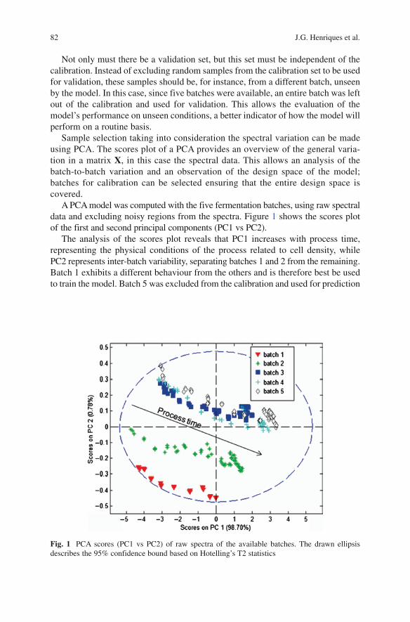
82 J.G. Henriques et al.
Not only must there be a validation set, but this set must be independent of the calibration. Instead of excluding random samples from the calibration set to be used for validation, these samples should be, for instance, from a different batch, unseen by the model. In this case, since five batches were available, an entire batch was left out of the calibration and used for validation. This allows the evaluation of the model’s performance on unseen conditions, a better indicator of how the model will perform on a routine basis.
Sample selection taking into consideration the spectral variation can be made using PCA. The scores plot of a PCA provides an overview of the general varia-tion in a matrix X, in this case the spectral data. This allows an analysis of the batch-to-batch variation and an observation of the design space of the model; batches for calibration can be selected ensuring that the entire design space is covered.
A PCA model was computed with the five fermentation batches, using raw spectral data and excluding noisy regions from the spectra. Figure 1 shows the scores plot of the first and second principal components (PC1 vs PC2).
The analysis of the scores plot reveals that PC1 increases with process time, representing the physical conditions of the process related to cell density, while PC2 represents inter-batch variability, separating batches 1 and 2 from the remaining. Batch 1 exhibits a different behaviour from the others and is therefore best be used to train the model. Batch 5 was excluded from the calibration and used for prediction
Fig. 1 PCA scores (PC1 vs PC2) of raw spectra of the available batches. The drawn ellipsis describes the 95% confidence bound based on Hotelling’s T2 statistics
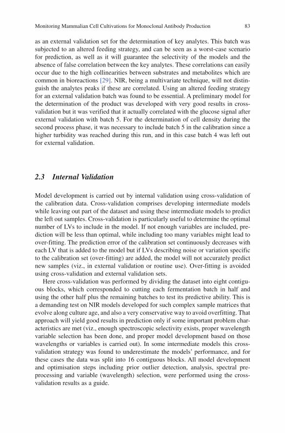
Monitoring Mammalian Cell Cultivations for Monoclonal Antibody Production 83
as an external validation set for the determination of key analytes. This batch was subjected to an altered feeding strategy, and can be seen as a worst-case scenario for prediction, as well as it will guarantee the selectivity of the models and the absence of false correlation between the key analytes. These correlations can easily occur due to the high collinearities between substrates and metabolites which are common in bioreactions [29]. NIR, being a multivariate technique, will not distin-guish the analytes peaks if these are correlated. Using an altered feeding strategy for an external validation batch was found to be essential. A preliminary model for the determination of the product was developed with very good results in cross-validation but it was verified that it actually correlated with the glucose signal after external validation with batch 5. For the determination of cell density during the second process phase, it was necessary to include batch 5 in the calibration since a higher turbidity was reached during this run, and in this case batch 4 was left out for external validation.
2.3 Internal Validation
Model development is carried out by internal validation using cross-validation of the calibration data. Cross-validation comprises developing intermediate models while leaving out part of the dataset and using these intermediate models to predict the left out samples. Cross-validation is particularly useful to determine the optimal number of LVs to include in the model. If not enough variables are included, pre-diction will be less than optimal, while including too many variables might lead to over-fitting. The prediction error of the calibration set continuously decreases with each LV that is added to the model but if LVs describing noise or variation specific to the calibration set (over-fitting) are added, the model will not accurately predict new samples (viz., in external validation or routine use). Over-fitting is avoided using cross-validation and external validation sets.
Here cross-validation was performed by dividing the dataset into eight contigu-ous blocks, which corresponded to cutting each fermentation batch in half and using the other half plus the remaining batches to test its predictive ability. This is a demanding test on NIR models developed for such complex sample matrices that evolve along culture age, and also a very conservative way to avoid overfitting. That approach will yield good results in prediction only if some important problem char-acteristics are met (viz., enough spectroscopic selectivity exists, proper wavelength variable selection has been done, and proper model development based on those wavelengths or variables is carried out). In some intermediate models this cross-validation strategy was found to underestimate the models’ performance, and for these cases the data was split into 16 contiguous blocks. All model development and optimisation steps including prior outlier detection, analysis, spectral pre-processing and variable (wavelength) selection, were performed using the cross-validation results as a guide.

84 J.G. Henriques et al.
Fig. 2 Raw spectra of a fermentation batch
2.4 Spectral Pre-Processing
Spectral pre-processing is commonly employed to reduce variations in the spectra not related to the parameters of interest and highlight the most relevant information. Spectral pre-processing reduces model complexity and provides robustness against unexpected perturbations. NIR spectra are sensitive to a number of variations such as random noise, baseline drift and light scattering among others. Applying a pre-processing method to the spectra guarantees that the modelling steps will focus on the relevant spectral features related to the parameters of interest.
Common pre-processing methods include first and second order derivatives (based on smoothing filters such as the SG), multiplicative scatter correction (MSC) and SNV (standard normal variate). A description of each of these methods and others can be found in the literature [40].
The raw spectra of a complete fermentation batch are presented in Fig. 2. The most notable feature observed in the spectra is the baseline shift increase with process time and two major bands corresponding to the water absorption regions around 5,000 and 7,000 cm−1. The baseline shift is caused by the increasing cell density of the medium which contributes to higher turbidity, increasing the light scatter and reducing the amount of light reaching the detector. If the parameter of interest is unrelated to cell density or another physical property, the effect of turbidity in the spectra should be removed. By applying a first derivative to the spectra, the baseline shift is removed and chemical information is highlighted allowing the modelling steps to ignore the physical information of the process. The first derivative of the same spectra are shown in Fig. 3.
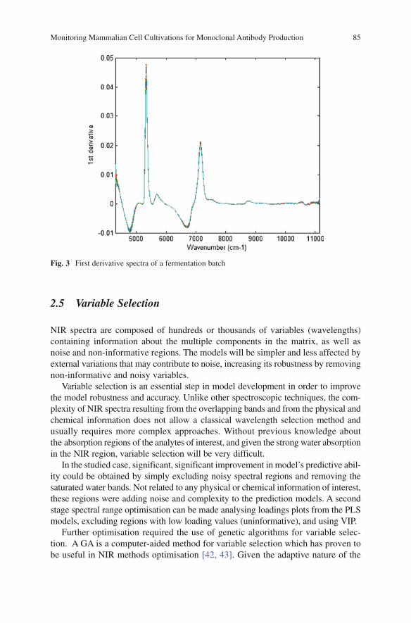
Monitoring Mammalian Cell Cultivations for Monoclonal Antibody Production 85
2.5 Variable Selection
NIR spectra are composed of hundreds or thousands of variables (wavelengths) containing information about the multiple components in the matrix, as well as noise and non-informative regions. The models will be simpler and less affected by external variations that may contribute to noise, increasing its robustness by removing non-informative and noisy variables.
Variable selection is an essential step in model development in order to improve the model robustness and accuracy. Unlike other spectroscopic techniques, the com-plexity of NIR spectra resulting from the overlapping bands and from the physical and chemical information does not allow a classical wavelength selection method and usually requires more complex approaches. Without previous knowledge about the absorption regions of the analytes of interest, and given the strong water absorption in the NIR region, variable selection will be very difficult.
In the studied case, significant, significant improvement in model’s predictive abil-ity could be obtained by simply excluding noisy spectral regions and removing the saturated water bands. Not related to any physical or chemical information of interest, these regions were adding noise and complexity to the prediction models. A second stage spectral range optimisation can be made analysing loadings plots from the PLS models, excluding regions with low loading values (uninformative), and using VIP.
Further optimisation required the use of genetic algorithms for variable selec-tion. A GA is a computer-aided method for variable selection which has proven to be useful in NIR methods optimisation [42, 43]. Given the adaptive nature of the
Fig. 3 First derivative spectra of a fermentation batch
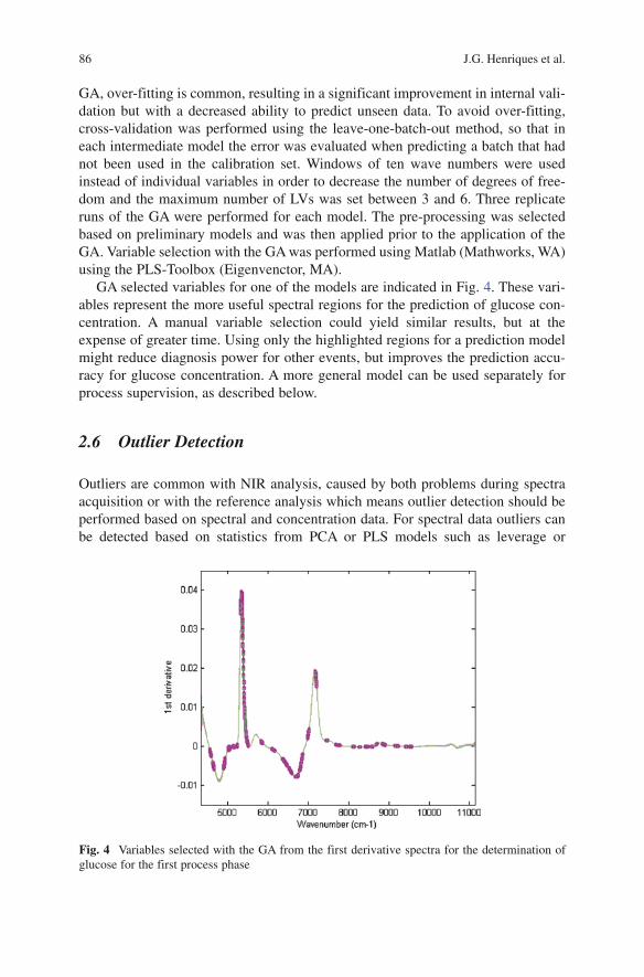
86 J.G. Henriques et al.
GA, over-fitting is common, resulting in a significant improvement in internal vali-dation but with a decreased ability to predict unseen data. To avoid over-fitting, cross-validation was performed using the leave-one-batch-out method, so that in each intermediate model the error was evaluated when predicting a batch that had not been used in the calibration set. Windows of ten wave numbers were used instead of individual variables in order to decrease the number of degrees of free-dom and the maximum number of LVs was set between 3 and 6. Three replicate runs of the GA were performed for each model. The pre-processing was selected based on preliminary models and was then applied prior to the application of the GA. Variable selection with the GA was performed using Matlab (Mathworks, WA) using the PLS-Toolbox (Eigenvenctor, MA).
GA selected variables for one of the models are indicated in Fig. 4. These vari-ables represent the more useful spectral regions for the prediction of glucose con-centration. A manual variable selection could yield similar results, but at the expense of greater time. Using only the highlighted regions for a prediction model might reduce diagnosis power for other events, but improves the prediction accu-racy for glucose concentration. A more general model can be used separately for process supervision, as described below.
2.6 Outlier Detection
Outliers are common with NIR analysis, caused by both problems during spectra acquisition or with the reference analysis which means outlier detection should be performed based on spectral and concentration data. For spectral data outliers can be detected based on statistics from PCA or PLS models such as leverage or
Fig. 4 Variables selected with the GA from the first derivative spectra for the determination of glucose for the first process phase
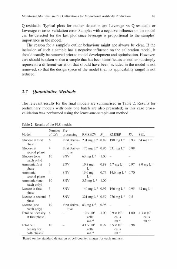
Monitoring Mammalian Cell Cultivations for Monoclonal Antibody Production 87
Q-residuals. Typical plots for outlier detection are Leverage vs Q-residuals or Leverage vs cross-validation error. Samples with a negative influence on the model can be detected for the last plot since leverage is proportional to the samples’ importance in the model.
The reason for a sample’s outlier behaviour might not always be clear. If the inclusion of such a sample has a negative influence on the calibration model, it should usually be removed prior to model development and optimisation. However, care should be taken so that a sample that has been identified as an outlier but simply represents a different variation that should have been included in the model is not removed, so that the design space of the model (i.e., its applicability range) is not reduced.
2.7 Quantitative Methods
The relevant results for the final models are summarised in Table 2. Results for preliminary models with only one batch are also presented; in this case cross-validation was performed using the leave-one-sample-out method.
Table 2 Results of the PLS models
ModelNumber of LVs
Pre-processing RMSECV R2
cvRMSEP R2
p SEL
Glucose at first phase
6 First deriva-tive
231 mg L−1 0.89 190 mg L−1 0.93 64 mg L−1
Glucose at second phase
4 First deriva-tive
175 mg L−1 0.96 331 mg L−1 0.88
Glucose (one batch only)
10 SNV 63 mg L−1 1.00 – –
Ammonia first phase
3 SNV 10.8 mg L−1
0.88 5.7 mg L−1 0.97 8.0 mg L−1
Ammonia second phase
4 SNV 13.0 mg L−1
0.74 14.6 mg L−1 0.70
Ammonia (one batch only)
10 SNV 3.5 mg L−1 1.00 – –
Lactate at first phase
5 SNV 140 mg L−1 0.97 196 mg L−1 0.95 42 mg L−1
Lactate at second phase
3 SNV 321 mg L−1 0.59 276 mg L−1 0.5
Lactate (one batch only)
10 First deriva-tive
83 mg L−1 0.98 – –
Total cell density at first phase
6 – 1.0 × 10⁵ cells mL−1
1.00 0.9 × 10⁵ cells mL−1
1.00 4.3 × 10⁵ cells mL−1a
Total cell density for both phases
10 – 4.1 × 10⁵ cells mL−1
0.97 3.5 × 10⁵ cells mL−1
0.98
a Based on the standard deviation of cell counter images for each analysis
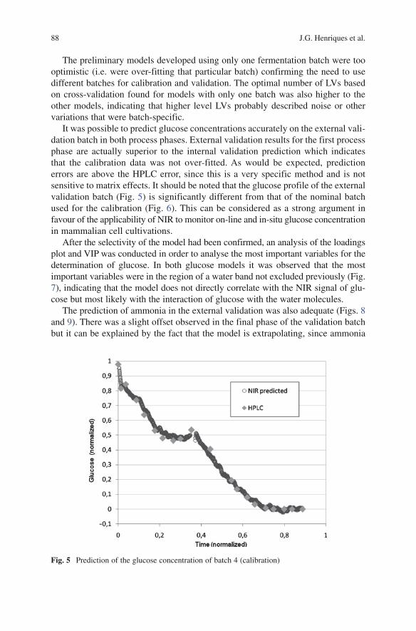
88 J.G. Henriques et al.
The preliminary models developed using only one fermentation batch were too optimistic (i.e. were over-fitting that particular batch) confirming the need to use different batches for calibration and validation. The optimal number of LVs based on cross-validation found for models with only one batch was also higher to the other models, indicating that higher level LVs probably described noise or other variations that were batch-specific.
It was possible to predict glucose concentrations accurately on the external vali-dation batch in both process phases. External validation results for the first process phase are actually superior to the internal validation prediction which indicates that the calibration data was not over-fitted. As would be expected, prediction errors are above the HPLC error, since this is a very specific method and is not sensitive to matrix effects. It should be noted that the glucose profile of the external validation batch (Fig. 5) is significantly different from that of the nominal batch used for the calibration (Fig. 6). This can be considered as a strong argument in favour of the applicability of NIR to monitor on-line and in-situ glucose concentration in mammalian cell cultivations.
After the selectivity of the model had been confirmed, an analysis of the loadings plot and VIP was conducted in order to analyse the most important variables for the determination of glucose. In both glucose models it was observed that the most important variables were in the region of a water band not excluded previously (Fig. 7), indicating that the model does not directly correlate with the NIR signal of glu-cose but most likely with the interaction of glucose with the water molecules.
The prediction of ammonia in the external validation was also adequate (Figs. 8 and 9). There was a slight offset observed in the final phase of the validation batch but it can be explained by the fact that the model is extrapolating, since ammonia
Fig. 5 Prediction of the glucose concentration of batch 4 (calibration)

Monitoring Mammalian Cell Cultivations for Monoclonal Antibody Production 89
production was significant in this batch due to an intentional change in the N-feeding strategy. This particular model seems to be affected by external condi-tions, given the appearance of noise-like features in the profile; further data would probably be required to increase the method’s robustness.
Fig. 6 Prediction of the glucose concentration of batch 5 (validation)
Fig. 7 Most relevant variables for the determination of glucose

90 J.G. Henriques et al.
The prediction of cell density was also adequate especially for the first phase. During the initial process phase, cell density is directly proportional to the turbidity of the medium. Subsequently at the start of the second phase this relation is lost with increasing cell lysis and a more complex model is required to predict cell density (10 LVS detected in this phase versus 6 in the initial phase). During the last
Fig. 9 Prediction of the ammonia concentration of batch 5 (validation)
Fig. 8 Prediction of the ammonia concentration of batch 4 (calibration)
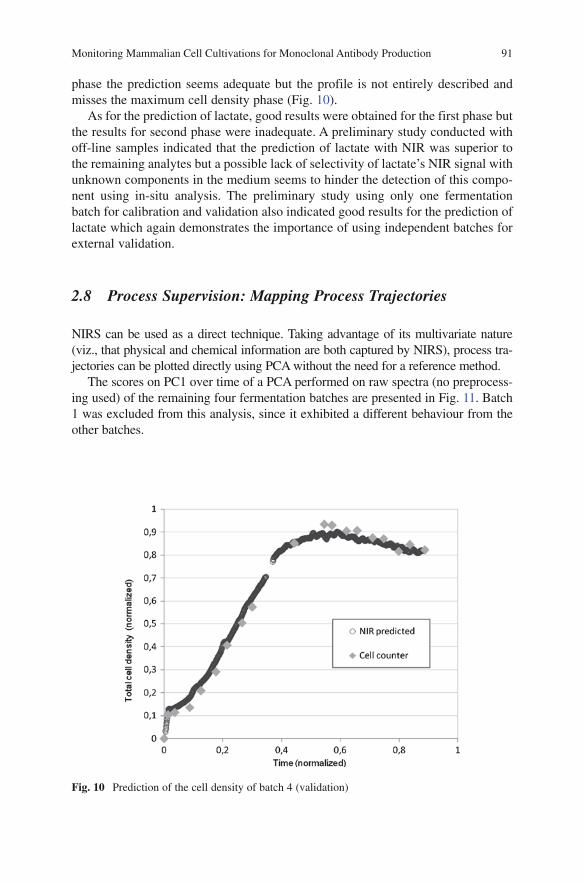
Monitoring Mammalian Cell Cultivations for Monoclonal Antibody Production 91
phase the prediction seems adequate but the profile is not entirely described and misses the maximum cell density phase (Fig. 10).
As for the prediction of lactate, good results were obtained for the first phase but the results for second phase were inadequate. A preliminary study conducted with off-line samples indicated that the prediction of lactate with NIR was superior to the remaining analytes but a possible lack of selectivity of lactate’s NIR signal with unknown components in the medium seems to hinder the detection of this compo-nent using in-situ analysis. The preliminary study using only one fermentation batch for calibration and validation also indicated good results for the prediction of lactate which again demonstrates the importance of using independent batches for external validation.
2.8 Process Supervision: Mapping Process Trajectories
NIRS can be used as a direct technique. Taking advantage of its multivariate nature (viz., that physical and chemical information are both captured by NIRS), process tra-jectories can be plotted directly using PCA without the need for a reference method.
The scores on PC1 over time of a PCA performed on raw spectra (no preprocess-ing used) of the remaining four fermentation batches are presented in Fig. 11. Batch 1 was excluded from this analysis, since it exhibited a different behaviour from the other batches.
Fig. 10 Prediction of the cell density of batch 4 (validation)
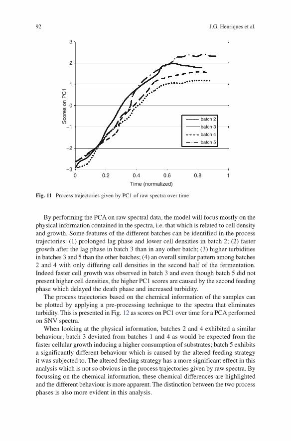
92 J.G. Henriques et al.
−3
−2
−1
0
0 0.2
Sco
res
on P
C1
Time (normalized)
batch 2
batch 3
batch 4
batch 5
0.4 0.6 0.8 1
1
2
3
Fig. 11 Process trajectories given by PC1 of raw spectra over time
By performing the PCA on raw spectral data, the model will focus mostly on the physical information contained in the spectra, i.e. that which is related to cell density and growth. Some features of the different batches can be identified in the process trajectories: (1) prolonged lag phase and lower cell densities in batch 2; (2) faster growth after the lag phase in batch 3 than in any other batch; (3) higher turbidities in batches 3 and 5 than the other batches; (4) an overall similar pattern among batches 2 and 4 with only differing cell densities in the second half of the fermentation. Indeed faster cell growth was observed in batch 3 and even though batch 5 did not present higher cell densities, the higher PC1 scores are caused by the second feeding phase which delayed the death phase and increased turbidity.
The process trajectories based on the chemical information of the samples can be plotted by applying a pre-processing technique to the spectra that eliminates turbidity. This is presented in Fig. 12 as scores on PC1 over time for a PCA performed on SNV spectra.
When looking at the physical information, batches 2 and 4 exhibited a similar behaviour; batch 3 deviated from batches 1 and 4 as would be expected from the faster cellular growth inducing a higher consumption of substrates; batch 5 exhibits a significantly different behaviour which is caused by the altered feeding strategy it was subjected to. The altered feeding strategy has a more significant effect in this analysis which is not so obvious in the process trajectories given by raw spectra. By focussing on the chemical information, these chemical differences are highlighted and the different behaviour is more apparent. The distinction between the two process phases is also more evident in this analysis.
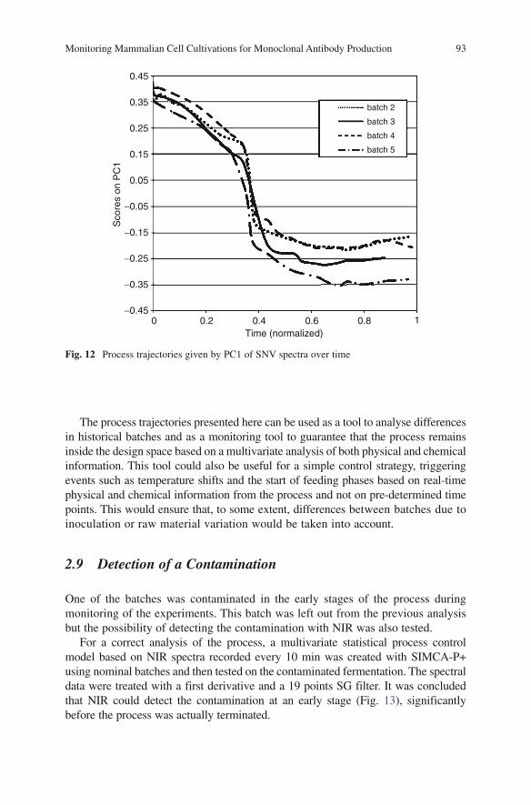
Monitoring Mammalian Cell Cultivations for Monoclonal Antibody Production 93
−0.45
−0.35
−0.25
−0.15
−0.05
0 0.2
Sco
res
on P
C1
Time (normalized)
batch 2
batch 3
batch 4
batch 5
0.4 0.6 0.8 1
0.05
0.15
0.25
0.35
0.45
Fig. 12 Process trajectories given by PC1 of SNV spectra over time
The process trajectories presented here can be used as a tool to analyse differences in historical batches and as a monitoring tool to guarantee that the process remains inside the design space based on a multivariate analysis of both physical and chemical information. This tool could also be useful for a simple control strategy, triggering events such as temperature shifts and the start of feeding phases based on real-time physical and chemical information from the process and not on pre-determined time points. This would ensure that, to some extent, differences between batches due to inoculation or raw material variation would be taken into account.
2.9 Detection of a Contamination
One of the batches was contaminated in the early stages of the process during monitoring of the experiments. This batch was left out from the previous analysis but the possibility of detecting the contamination with NIR was also tested.
For a correct analysis of the process, a multivariate statistical process control model based on NIR spectra recorded every 10 min was created with SIMCA-P+ using nominal batches and then tested on the contaminated fermentation. The spectral data were treated with a first derivative and a 19 points SG filter. It was concluded that NIR could detect the contamination at an early stage (Fig. 13), significantly before the process was actually terminated.
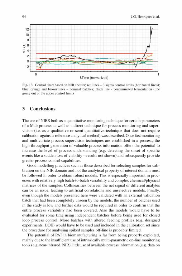
94 J.G. Henriques et al.
3 Conclusions
The use of NIRS both as a quantitative monitoring technique for certain parameters of a Mab process as well as a direct technique for process monitoring and super-vision (i.e. as a qualitative or semi-quantitative technique that does not require calibration against a reference analytical method) was described. Once fast monitoring and multivariate process supervision techniques are established in a process, the high-throughput generation of valuable process information offers the potential to increase the level of process understanding (e.g. detecting the onset of specific events like a sudden loss of viability – results not shown) and subsequently provide greater process control capabilities.
Good modelling practices such as those described for selecting samples for cali-bration on the NIR domain and not the analytical property of interest domain must be followed in order to obtain robust models. This is especially important in proc-esses with relatively high batch-to-batch variability and complex chemical/physical matrices of the samples. Collinearities between the net signal of different analytes can be an issue, leading to artificial correlations and unselective models. Finally, even though the models presented here were validated with an external validation batch that had been completely unseen by the models, the number of batches used in the study is low and further data would be required in order to confirm that the entire process variability had been covered. Also the models would have to be evaluated for some time using independent batches before being used for closed loop process control. More batches with altered feeding profiles (e.g. designed experiments, DOE) would have to be used and included in the calibration set since the procedure for analysing spiked samples off-line is probably limited.
The potential of PAT in biomanufacturing is far from being properly exploited, mainly due to the insufficient use of intrinsically multi-parametric on-line monitoring tools (e.g. near-infrared, NIR), little use of available process information (e.g. data on
$Time (normalized)10
0
2
4
6
tPS
[1]
8
10
12
−2
Fig. 13 Control chart based on NIR spectra; red lines – 3 sigma control limits (horizontal lines); blue, orange and brown lines – nominal batches; black line - contaminated fermentation (line going out of the upper control limit)

Monitoring Mammalian Cell Cultivations for Monoclonal Antibody Production 95
historical batches and data collected at different process stages such as inocula development and raw-material lots) and lack of a process/plant wide perspective for the proposed PAT strategy.
Acknowledgments Dr Licinia O. Rodrigues (4TUNE Engineering Ltd) for discussions on the material in the paper. Mrs Miriam Ahlert (Roche Diagnostics GmbH, Germany) for support in the analytical work.
References
1. Lopes JA, Costa PF, Alves TP, Menezes JC (2004) Chemometrics in bioprocess engineering: process analytical technology (PAT) applications. Chemometr Intell Lab Syst 74:269–275
2. Menezes JC, Ferreira AP, Rodrigues LO, Brás LP, Alves TP (2009) Chemometrics role within the PAT context: examples from primary pharmaceutical manufacturing. In: Steve B, Romà T, Beata W (eds) Comprehensive chemometrics, chap 13.11, 4 vols. Elsevier, Amsterdam
3. Scarff M, Arnold SA, Harvey LM, McNeil B (2006) Near infrared spectroscopy for bioprocess monitoring and control: current status and future trends. Crit Rev Biotechnol 26:17–39
4. Rodrigues LO Cardoso JP, Menezes JC (2005) From lab to plant: a scale-independent NIR calibration to monitor an ionic exchange column. Chemometr Intell Lab Syst 75(1):101–108
5. Rodrigues LO, Cardoso JP, Menezes JC (2008) Applying Near Infrared Spectroscopy in downstream processing:one calibration for multiple clarification processes of fermentation media. Biotechnol Prog 24(2):432–435
6. FDA (2004) Guidance for industry PAT – a framework for innovative pharmaceutical devel-opment, manufacturing, and quality assurance, September 2004
7. ICH (2008) Guideline Q8 – pharmaceutical development, November 2008 8. Kourti T (2004) Process analytical technology and multivariate statistical process control.
Wellness Index of process and product (Part 1). J Process Anal Technol 1(1):13–19 9. Kourti T (2005) Process analytical technology and multivariate statistical process control.
Wellness Index of process and product (Part 2). J Process Anal Technol 2(1):24–28 10. Kourti T (2006) Process analytical technology and multivariate statistical process control.
Wellness Index of process and product (Part 3). J Process Anal Technol 3(1):18–24 11. Montague G (1997) Monitoring and control of fermentors. Institution of Chemical Engineers,
Rugby, UK 12. Herschel W (1800), Investigation of the power of the prismatic colours to heat and illuminate
objects. Philos Trans R Soc 90:255–283 13. Williams P, Norris K (eds) (2001) Near-infrared technology in the agricultural and food
industries. American Association of Cereal Chemists, St Paul, MN, USA 14. McClure WF (1994) Near-infrared spectroscopy: the giant is running strong. Anal Chem
66:43A–53A 15. Ciurczak EW, Drennen JK (2002) Pharmaceutical and medical applications of near-infrared
spectroscopy. Marcel Dekker, New York 16. McClure WF (2003) 204 years of near infrared technology: 1800–2003. J Near Infrared
Spectrosc 11:487–518 17. Bakeev KA (ed) (2005) Process analytical technology. Blackwell, Oxford 18. Reich G (2005) Near-infrared spectroscopy and imaging: basic principles and pharmaceutical
applications. Adv Drug Deliv Rev 57:1109–1143 19. Siesler HW, Ozaki Y, Kawata S, Heise HM (eds) (2002) Near-infrared spectroscopy: princi-
ples, instruments, applications. Wiley, Weinheim, Germany 20. Ozaki Y, Amari T (2000) Near-infrared spectroscopy in chemical process analysis. In: Chalmers
JM (ed) Spectroscopy in process analysis. Sheffield Academic, Sheffield, UK, pp 53–95
96 J.G. Henriques et al.
21. Raghavachari R (ed) (2001) Near-infrared applications in biotechnology. Marcel Dekker, New York, USA
22. Silman RW, Black LT, Norris K (1983) Assay of solid-substrate fermentation by means of reflectance infrared analysis. Biotechnol Bioeng 25:603–607
23. Cavinato AG, Mayes DM, Ge Z, Callis JB (1990) Non-invasive method for monitoring ethanol in fermentation processes using fibre-optic near-infrared spectroscopy. Anal Chem 62:1977–1982
24. Ge Z, Cavinato AG, Callis JB (1994) Non-invasive spectroscopy for monitoring cell density in a fermentation process. Anal Chem 66:1354–1362
25. Blanco M, Peinado AC, Mas J (2004) Analytical monitoring of alcoholic fermentation using NIR spectroscopy. Biotechnol Bioeng 88:536–542
26. González-Vara A, Vaccari G, Dosi E, Trilli A, Rossi M, Matteuzzi D (2000) Enhanced pro-duction of L-(+)- lactic acid in chemostat by Lactobacillus casei DSM 20011 using ion-exchange resins and cross-flow filtration in a fully automated pilot plant controlled via NIR. Biotechnol Bioeng 67:47–156
27. Vaccari G, Dosi E, Campi A, Mantovani G, González-Varay R A, Matteuzzi D (1994) A NIR spectroscopy technique for the control of fermentation processes: an application to lactic acid fermentation. Biotechnol Bioeng 43:913–917
28. Arnold SA, Crowley J, Woods N, Harvey LM, McNeil B (2003) In-situ near infrared spec-troscopy to monitor key analytes in mammalian cell cultivation. Biotechnol Bioeng 84:13–19
29. Rhiel M, Cohen MB, Murhammer DW, Arnold MA (2002) Nondestructive near-infrared spectroscopic measurement of multiple analytes in undiluted samples of serum-based cell culture media. Biotechnol Bioeng 77:73–82
30. Riley MR, Okeson CD, Frazier BL (1999) Rapid calibration of near-infrared spectroscopic measurements of mammalian cell cultivations. Biotechnol Progr 15:1133–1141
31. Riley MR, Rhiel M, Zhou X, Arnold MA, Murhammer DW (1997) Simultaneous measure-ment of glucose and glutamine in insect cell culture media by near infrared spectroscopy. Biotechnol Bioeng 55:11–15
32. Arnold SA, Gaensakoo R, Harvey LM, McNeil B (2002) Use of at-line and in-situ near-infrared spectroscopy to monitor biomass in an industrial fed-batch Escherichia coli process. Biotechnol Bioeng 80:405–413
33. Macaloney G, Hall JW, Rollins MJ, Draper I, Anderson KB, Preston J, Thompson BG, McNeil B (1997) The utility and performance of near-infra red spectroscopy in simultaneous monitoring of multiple components in a high cell density recombinant Escherichia coli pro-duction process. Bioprocess Biosyst Eng 17:157–167
34. Crowley J, Arnold SA, Wood N, Harvey LM, McNeil B (2005) Monitoring a high cell density recombinant Pichia pastoris fed-batch bioprocess using transmission and reflectance near infrared spectroscopy. Enzyme Microb Technol 36:621–628
35. Arnold SA, Crowley J, Vaidyanathan S, Matheson L, Mohan P, Hall JW, Harvey LM, McNeil B (2000) At-line monitoring of a submerged filamentous bacterial cultivation using near-infrared spectroscopy. Enzyme Microb Technol 27:691–697
36. Vaidyanathan S, Macaloney G, Harvey LM, McNeil B (2001) Assessment of the structure and predictive ability of models developed for monitoring key analytes in a submerged fungal bioprocess using near-infrared spectroscopy. Appl Spectrosc 55:444–453
37. Chen T, Martin E (2007) The impact of temperature variations on spectroscopic calibration modelling: a comparative study. J Chemometr 21:198–207
38. Segtnan VH, Mevik B-H, Isaksson T, Næs T (2005) Low-cost approaches to robust tempera-ture compensation in near-infrared calibration and prediction situations. Appl Spectrosc 59:816–825
39. Wülfert F (2004) Temperature-robust multivariate calibration, Phd Thesis (English 135 pp), University of Amsterdam, The Netherlands, available online http://dare.uva.nl/record/161626 (accessed June 13, 2008)

Monitoring Mammalian Cell Cultivations for Monoclonal Antibody Production 97
40. Næs T, Isaksson T, Fearn T, Davies T (2002) A user-friendly guide to multivariate calibration and classification. NIR, Chichester
41. Otto M (1999) Chemometrics: statistics and computer application in analytical chemistry. Wiley, Chichester
42. Ferreira A, Menezes J (2005) Monitoring complex media fermentations with near-infrared spectroscopy: comparison of different variable selection methods. Biotechnol Bioeng 91:4
43. Leardi R (2000) Application of genetic algorithm-PLS for feature selection in spectral data sets. J Chemometr 14:643–655
Environmental Applications of Photoluminescence-Based Biosensors
Kenneth F. Reardon, Zhong Zhong, and Kevin L. Lear
Abstract For monitoring and treatment of soil and water, environmental scientists and engineers require measurements of the concentration of chemical contaminants. Although laboratory-based methods relying on gas or liquid chromatography can yield very accurate measurements, they are also complex, time consuming, expensive, and require sample pretreatment. Furthermore, they are not readily adapted for in situ measurements.
Sensors are devices that can provide continuous, in situ measurements, ideally without the addition of reagents. A biosensor incorporates a biological component coupled to a transducer, which translates the interaction between the analyte and the biocomponent into a signal that can be processed and reported. A wide range of transducers have been employed in biosensors, the most common of which are electrochemical and optical. In this contribution, we focus on photoluminescence-based biosensors of potential use in the applications described above.
Following a review of photoluminescence and a discussion of the optoelectronic hardware part of these biosensor systems, we provide explanations and examples of optical biosensors for specific chemical groups: hydrocarbons and alcohols, halogenated organics, nitro-, phospho-, sulfo-, and other substituted organics, and metals and other inorganics. We also describe approaches that have been taken to describe chemical mixtures as a whole (biological oxygen demand and toxicity) since most environmental samples contain mixtures of unknown (and changing)
K.F. Reardon () and Z. ZhongDepartment of Chemical and Biological Engineering, Colorado State University, Fort Collins, CO, USAe-mail: [email protected]
K.L. LearDepartment of Electrical and Computer Engineering, Colorado State University, Fort Collins, CO, USA
Adv Biochem Engin/Biotechnol (2009) 116: 99–123DOI: 10.1007/10_2008_51© Springer-Verlag Berlin Heidelberg 200Published online: 21 May 2009
9
100 K.F. Reardon et al.
1 Introduction ......................................................................................................................... 100 1.1 Photoluminescence-Based Biosensors ....................................................................... 100 1.2 Environmental Applications for Biosensors ............................................................... 101 1.3 Scope .......................................................................................................................... 1022 Characteristics and Challenges of Environmental Measurements ....................................... 1033 Optoelectronic Hardware ..................................................................................................... 103 3.1 Optical Biosensors ...................................................................................................... 103 3.2 Instrumentation Components ..................................................................................... 105 3.3 Photoluminescence Apparatus .................................................................................... 107 3.4 Multiplexed Fiber Optic Biosensor Systems .............................................................. 1094 Biosensors for Chemical Analytes ....................................................................................... 111 4.1 Hydrocarbons and Alcohols ....................................................................................... 111 4.2 Halogenated Organics ................................................................................................ 113 4.3 Nitro-, Phospho-, Sulfo-, and Other Substituted Organics ......................................... 117 4.4 Metals and Other Inorganics ...................................................................................... 118 4.5 Chemical Mixtures ..................................................................................................... 1195 Summary and Future Developments .................................................................................... 120References .................................................................................................................................. 122
composition. Finally, we end with some thoughts on future research directions that are necessary to achieve the full potential of environmental biosensors.
Keywords Antibody • Biosensors • Enzyme • Induction
1 Introduction
1.1 Photoluminescence-Based Biosensors
Environmental scientists and engineers frequently desire to measure the concentration of chemical contaminants in soil and water samples. Although laboratory-based methods relying on gas or liquid chromatography can yield very accurate measure-ments, they are also complex, time consuming, require sample pretreatment, and use expensive equipment. Furthermore, obtaining measurements directly at the source of the sample is often important, but modifying chromatographic methods for field use has proven to be difficult.
To overcome these limitations, researchers have developed a variety of assays and sensors for environmental contaminants. Immunoassays have been developed for field use, particularly for larger analytes such as polycyclic aromatic hydro-carbons [1] and chlorinated pesticides [2]. However, these assays provide only a single measurement each, cannot be used in situ (and thus are subject to sampling errors), require reagents and several analytical steps, and suffer from poor specificity for smaller molecules.

Environmental Applications of Photoluminescence-Based Biosensors 101
Sensors are devices that can provide continuous, in situ measurements, ideally without the addition of reagents. A biosensor is a device in which a biological component (typically an enzyme or antibody) is coupled to a transducer, which essentially translates the interaction between the analyte and the biocomponent into a signal that can be processed and reported. A wide range of transducers have been employed in biosensors, the most common of which are electrochemical and optical.
In this review, we focus on biosensors in which photoluminesence serves as the transduction mechanism. Optical biosensors in general have advantages over those relying on other transduction methods. These desirable characteristics include small size, the ability to measure over long distances with minimal signal loss, and no requirement for reference cells/sensors. In addition, photoluminescence-based biosensors have the ability to achieve higher sensitivity with lower interference from other sample components than is the case with absorbance or other types of optical biosensors. Photoluminesence transducers can be coupled to a variety of biocom-ponents, including enzymes (purified and in whole cells), antibodies, aptamers, and whole cells and tissues. The majority of reported photoluminescence-based biosensors have used enzymes. Antibodies are more commonly used in bioassays because of the need in most detection formats to add reagents and wash the reactive surface, but a few biosensors have been described in which these steps have been modified to allow semicontinuous measurements.
1.2 Environmental Applications for Biosensors
The range of application scenarios for biosensors in environmental science and engineering is broad, but in general two categories of measurement goals can be proposed. First, measurements may be made initially to assess and characterize the types and levels of contaminants at a particular site or in a body of water. In this case, only one time point may be desired (although different locations are normally evaluated), and often there is little previous information about the contaminants at the site. The second goal is monitoring. In this case, the objective is to track the concentration of known contaminants over time at one or more defined locations. To date, these monitoring measurements have consisted of a series of discrete meas-urements (assays). However, biosensors, with their ability to provide continuous, or high frequency semicontinuous, measurements, offer the potential for more information about these contaminant levels.
Examples of some application scenarios are:
• Water treatment process monitoring. In both drinking water and wastewater treatment processes it is desirable to monitor contaminant levels for the protection of human and environmental health. Given the very high flow rates of these processes, continuous monitoring of specific chemicals would be desirable; however, but this is not possible with currently available technology.
• Protection from chemical terrorism of water supplies. The possibility of terrorist attacks by the addition of chemicals to water supplies has arisen in recent years.
102 K.F. Reardon et al.
Low cost, continuous measurements of specific chemicals or of toxicity would protect people from this danger.
• Characterization of contaminated sites. When soil and/or groundwater contami-nation is suspected at a site, the type and level of contaminants at the site must be profiled so that an effective remediation strategy can be developed. Using laboratory-based measurements requires the removal of samples and a waiting period before data are obtained, and then several additional rounds of sampling and analysis are usually needed. The use of biosensors for this initial assessment phase would enable the site to be completely characterized in one sweep, potentially saving both time and money.
• Monitoring of remediation processes. Once a remediation process has been designed and implemented at a contaminated site, its effectiveness must be established through a program of periodic monitoring. This could be performed with biosensors on site, either in the assay mode or as part of a continuous monitoring system.
• Environmental monitoring. It is often desirable to monitor sensitive water sources (ground water wells, rivers, lakes, etc.) that are downgradient from industrial sites and other sources of contaminants. Traditional manual sampling and laboratory analysis are too expensive and too slow to accomplish this monitoring goal, but biosensors that can measure continuously and in situ could play an important role in this application.
• Precision agriculture. The goal of precision agriculture is to apply the correct amount of fertilizer and pesticide on every portion of a field, recognizing that different amounts are required depending on slope, exposure, soil type, and other factors. The use of in situ biosensors would provide feedback to farmers about these chemical application rates.
In all of these scenarios, biosensors could provide important information not readily available using traditional analytical technologies, particularly when continuous or in situ measurements are desired. Biosensor and traditional technologies could also be paired, with biosensors used on site for immediate data acquisition and traditional measurements performed later in a laboratory with high accuracy methods.
1.3 Scope
Several general reviews on biosensors for environmental applications were published in the 1990s [3, 4]. In this contribution, we focus on photoluminesence-based biosensors of potential use in the applications described above. In general, only reports of biosensors are included, although some assays are mentioned when it is evident that the underlying measurement technology could be modified to yield continuous, in situ data. In addition to chemical-specific biosensors, we consider those that report an assessment of toxicity.
Environmental Applications of Photoluminescence-Based Biosensors 103
2 Characteristics and Challenges of Environmental Measurements
Analyte concentration measurement in any practical application faces numerous challenges; for example, sensors must be robust, free of interferences from chemical, physical, or biological factors, and retain activity for a long period. However, measurements in surface or ground water matrices have additional attributes that provide challenges for biosensor development, especially in the case of in situ measurements. Some of these are:
• Wide range of analytes. Contaminated ground water, waste water, and other environmental samples usually contain many different analytes of interest.
• Low analyte concentrations. In contrast to analytes in industrial bioprocesses, in which the relevant concentration range is usually in the mgL−1 to gL−1 range, concentrations of interest in environmental samples are dictated by governmental health regulations and are typically around 1 mg L−1 or less. Traditional measure-ment methods rely upon a concentration step to achieve these low limits of quantitation, but biosensors must be capable of high sensitivity without sample pretreatment.
• Complex matrices. Environmental samples are frequently complex in chemical, biological, and/or physical terms. The presence of soil particles, soil organic matter, microorganisms, salts, nonanalyte organics and metals, and other factors are challenging for biosensor development, and the range of these factors in different samples makes the development of robust calibration protocols a vital consideration.
• Demands of field applications. Equipment intended for use at a site (rather than in a laboratory or process environment) must be durable and not shock sensitive, must not require an external power source, and must not be affected by heat, cold, direct sunlight, wind, and other factors.
• Expectations for low cost. Because environmental measurements are performed in a regulation-driven context and not a profit-driven one, measurements and measurement equipment are expected to be inexpensive and to have a long life.
3 Optoelectronic Hardware
3.1 Optical Biosensors
Optical sensing encompasses an enormous field of technology with applications spanning from imaging to spectroscopy on scales from astronomical ranging to subwavelength interferometry. At the core of optical sensing is metrology of one of the fundamental parameters of electromagnetic waves: phase, polarization, or most commonly, amplitude. With reference to Fig. 1, amplitude measurements relevant
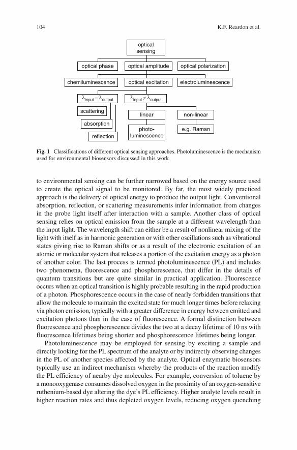
104 K.F. Reardon et al.
to environmental sensing can be further narrowed based on the energy source used to create the optical signal to be monitored. By far, the most widely practiced approach is the delivery of optical energy to produce the output light. Conventional absorption, reflection, or scattering measurements infer information from changes in the probe light itself after interaction with a sample. Another class of optical sensing relies on optical emission from the sample at a different wavelength than the input light. The wavelength shift can either be a result of nonlinear mixing of the light with itself as in harmonic generation or with other oscillations such as vibrational states giving rise to Raman shifts or as a result of the electronic excitation of an atomic or molecular system that releases a portion of the excitation energy as a photon of another color. The last process is termed photoluminescence (PL) and includes two phenomena, fluorescence and phosphorescence, that differ in the details of quantum transitions but are quite similar in practical application. Fluorescence occurs when an optical transition is highly probable resulting in the rapid production of a photon. Phosphorescence occurs in the case of nearly forbidden transitions that allow the molecule to maintain the excited state for much longer times before relaxing via photon emission, typically with a greater difference in energy between emitted and excitation photons than in the case of fluorescence. A formal distinction between fluorescence and phosphorescence divides the two at a decay lifetime of 10 ns with fluorescence lifetimes being shorter and phosphorescence lifetimes being longer.
Photoluminescence may be employed for sensing by exciting a sample and directly looking for the PL spectrum of the analyte or by indirectly observing changes in the PL of another species affected by the analyte. Optical enzymatic biosensors typically use an indirect mechanism whereby the products of the reaction modify the PL efficiency of nearby dye molecules. For example, conversion of toluene by a monooxygenase consumes dissolved oxygen in the proximity of an oxygen-sensitive ruthenium-based dye altering the dye’s PL efficiency. Higher analyte levels result in higher reaction rates and thus depleted oxygen levels, reducing oxygen quenching
Fig. 1 Classifications of different optical sensing approaches. Photoluminescence is the mechanism used for environmental biosensors discussed in this work
linput ≠ loutputlinput = loutput
scattering
reflection
absorption
non-linearlinear
e.g. Ramanphoto-luminescene
optical sensing
optical polarization
electroluminescenceoptical excitation
optical phase optical amplitude
scattering
reflection
absorption
non-linearlinear
e.g. Ramanphoto-luminescence
opticalsensing
optical polarization
chemiluminescence electroluminescenceoptical excitation
Environmental Applications of Photoluminescence-Based Biosensors 105
of the ruthenium dye and increasing the associated phosphorescence emission under constant excitation power.
3.2 Instrumentation Components
A variety of optoelectronic options are available for sources and detectors to provide an interface between electronic power supplies and signal processing and the optical realm in which PL sensing occurs. In conventional linear photoluminescence (as opposed to two-photon excited PL), the optical source must deliver a sufficient amount of excitation power in the absorption band of the photoluminescent material, which will be at higher energy and thus shorter wavelength than the material’s emission peak. Most fluorescent and phosphorescent dyes have been developed to emit in the visible spectrum due to the limited response of conventional photomultiplier cathode materials, e.g., S-1, at longer, infrared wavelengths. Thus PL sources emitting in the blue to ultraviolet portion of the spectrum are appropriate for many dyes. Efficient, durable, and compact modern sources in this range are typically light-emitting diodes (LEDs) and laser diodes based on GaN and related III–V semiconductors, although SiC LEDs and halogen lamps were designed into earlier systems. Compared to LEDs, laser diodes provide much greater energy efficiency, higher power, more intense and readily focused output beams, an output spectrum less than 1 nm wide, and the potential for polarized operation. Laboratory-grade blue laser diodes are still 10–100 times more expensive than comparable red laser diodes, but spin-off technology from Blu-ray disc players should virtually eliminate this difference within a few years. Lower cost is the major advantage of blue LEDs with instrumentation grade devices in molded plastic housings that offer direct fiber connections selling on the order of US$10 in small volumes, slightly less than the cost of laboratory red laser diodes. Direct fiber coupling of LEDs, practically eliminates the advantages of laser diode beam properties relative to LEDs and dye photobleaching at high optical intensities [5] can restrict the ability to fully leverage the higher output powers of laser diodes. With proper drive electronics, LEDs can operate at or near the shot noise limit, while laser diodes frequently exhibit noise at least ten times the shot noise limit although designers should recall that the shot noise limited electrical signal-to-noise ratio is proportional to optical power. The output spectrum of many blue LEDs is approximately 20 nm full-width at half-maximum and contains long tails often necessitating the use of a source bandpass filter to block excitation light falling in the PL emission band. The ratio of peak-to-tail power from laser diodes at high drive currents is much better than LEDs, but the corresponding high power may require a neutral density filter or other component to attenuate the total power.
Akin to the replacement of blue lamps with GaN diodes, advances in semiconductor technology provide alternatives to traditional photomultiplier tubes (PMTs) for sensitive conversion of emitted light into an electronic signal although they are not yet as competitive. While simple silicon photodiodes can efficiently convert incident
106 K.F. Reardon et al.
photons into electron flow, the resulting photocurrents often fall below the noise floor of subsequent amplification electronics when attempting to detect faint emission from PL. PMTs are advantageous in this situation as their internal gain results in an internally amplified photocurrent above the electronic amplifier noise floor although the internal gain results in a reduced signal-to-noise ratio as does any amplification process. PMT operation in instruments has been significantly simplified through the integration of high voltage generation subsystems so that the instrument only needs to provide standard low voltages, e.g., 12 V, to the PMT module. PMTs are typically the most expensive single component in PL sensor instrumentation with costs on the order of US$1,000. Solid-state replacements for the PMT, avalanche photodiodes (APDs), are becoming more frequently employed, although they do not yet rival PMT performance. Compared to PMTs, typical APDs have somewhat higher noise factors, an order of magnitude higher dark current, and a factor of a thousand or more lower internal gain [6]. APDs are more compact and robust than PMTs. Relatively high prices for APD modules, near those for PMTs, are currently supported by market factors although silicon based APDs should eventually be manufactured at much lower costs than PMTs. Another lower performance solid-state alternative to the PMT is the p–i–n silicon photodiode with hybrid integrated transimpedance amplifier (PIN–TIA) that combines the photodiode and a low noise electronic amplifier in a package size comparable to those used for the photodiode alone. PIN–TIAs require more optical power than APDs and PMTs to produce a signal equivalent to their noise but perform better than discrete integrations of photodiodes with external amplifiers. In low volumes they sell for approximately one-tenth the price of PMTs. For PL sensor systems where low limits of detection are more important than minimal cost or minimal size, PMTs remain the detector of choice for the present.
Beyond the components that convert electrical power to light or light to electrical signals, optical elements such as fibers and filters are required to control optical propagation and block undesired wavelengths. Optical fibers provide a convenient means for transporting excitation light to and returning emitted light from PL sensors. They eliminate the need to maintain optical alignment through much of the system and allow optical sensing at points interior to the analyte volume. Maximization of collected light in PL-based fiber optic sensor systems is paramount and drives the use of fibers with very large core diameters, ~1 mm. Although silica fibers with core diameters ranging from approximately 5 to 50 mm are preferred for most communications applications over distances greater than 10 m, a 1 mm diameter silica fiber would have an impractically large bending radius. Instead, large core plastic fibers manufactured from PMMA are routinely used for sensors. The light acceptance cone, parameterized with the numerical aperture, is usually designed to be much larger in plastic fibers than for glass by using a 5% refractive index step between the core and cladding to achieve numerical apertures as large as 0.5. Plastic fibers are readily available with either SMA- or ST-style terminations where the latter may be preferred due to the presence of an air gap in SMA connections that can result in optical interference. A disadvantage of plastic fibers is their increased absorption over silica fibers. PMMA-based fibers present optical losses
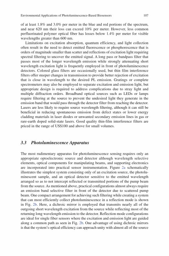
Environmental Applications of Photoluminescence-Based Biosensors 107
of at least 1.8% and 3.0% per meter in the blue and red portions of the spectrum, and near 620 nm their loss can exceed 10% per meter. However, less common perfluorinated polymer optical fiber has losses below 1.4% per meter for visible wavelengths greater than 600 nm.
Limitations on excitation absorption, quantum efficiency, and light collection often result in the need to detect emitted fluorescence or phosphorescence that is orders of magnitude smaller than scatter and reflections of excitation light requiring spectral filtering to uncover the emitted signal. A long pass or bandpass filter that passes most of the longer wavelength emission while strongly attenuating short wavelength excitation light is frequently employed in front of photoluminescence detectors. Colored glass filters are occasionally used, but thin film interference filters offer steeper changes in transmission to provide better rejection of excitation that is close in wavelength to the desired PL emission. Gratings or complete spectrometers may also be employed to separate excitation and emission light, but appropriate design is required to address complications due to stray light and multiple diffraction orders. Broadband optical sources such as LEDs or lamps require filtering at the source to prevent the undesired light they generate in the emission band that would pass through the detector filter from reaching the detector. Lasers are less likely to require source wavelength filtering, although it can still be beneficial in reducing spontaneous emission from defect states or lower energy cladding materials in laser diodes or unwanted secondary emission lines in gas or rare-earth doped solid-state lasers. Good quality thin-film interference filters are priced in the range of US$100 and above for small volumes.
3.3 Photoluminescence Apparatus
The most rudimentary apparatus for photoluminescence sensing requires only an appropriate optoelectronic source and detector although wavelength selective elements, optical components for manipulating beams, and supporting electronics are incorporated into practical sensor instrumentation. Figure 2a schematically illustrates the simplest system consisting only of an excitation source, the photolu-minescent sample, and an optical detector sensitive to the emitted wavelength arranged so as to not intercept reflected or transmitted portions of the pump beam from the source. As mentioned above, practical configurations almost always require an emission band selective filter in front of the detector due to scattered pump beam. One compact arrangement for achieving such filtering while creating a system that can most efficiently collect photoluminescence in a reflection mode is shown in Fig. 2b. Here, a dichroic mirror is employed that transmits nearly all of the outgoing short wavelength excitation from the source while reflecting most of the returning long wavelength emission to the detector. Reflection mode configurations are ideal for single fiber sensors where the excitation and emission light are guided along a common path as seen in Fig. 2b. One advantage of using dichroic mirrors is that the system’s optical efficiency can approach unity with almost all of the source
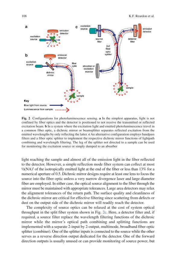
108 K.F. Reardon et al.
light reaching the sample and almost all of the emission light in the fiber reflected to the detector. However, a simple reflection mode fiber system can collect at most ½(NA)2 of the isotropically emitted light at the end of the fiber or less than 13% for a numerical aperture of 0.5. Dichroic mirror designs require at least one lens to focus the source into the fiber optic unless a very narrow divergence laser and large diameter fiber are employed. In either case, the optical source alignment to the fiber through the mirror must be maintained with appropriate tolerances. Large area detectors may relax the alignment tolerances of the return path. The surface quality and cleanliness of the dichroic mirror are critical for effective filtering since scattering from defects or dust on the output side of the dichroic mirror will readily reach the detector.
The complexity of source optics can be relaxed at the cost of system optical throughput in the split fiber system shown in Fig. 2c. Here, a detector filter and, if required, a source filter replace the wavelength filtering functions of the dichroic mirror while the mirror’s optical path combining and splitting functions are implemented with a separate 2-input by 2-output, multimode, broadband fiber optic splitter (combiner). One of the splitter inputs is connected to the source while the other serves as a reverse direction output dedicated for the detector. One of the forward direction outputs is usually unused or can provide monitoring of source power, but
Fig. 2 Configurations for photoluminescence sensing. a In the simplest apparatus, light is not confined by fiber optics and the detector is positioned to not receive the transmitted or reflected excitation beam. b In a system where the excitation light and emitted photoluminescence travel in a common fiber optic, a dichroic mirror or beamsplitter separates reflected excitation from the emitted wavelengths by only reflecting the latter. c An alternative configuration employs bandpass filters and a fiber optic splitter to implement the respective dichroic mirror functions of lightpath combining and wavelength filtering. The leg of the splitter not directed to a sample can be used for monitoring the excitation source or simply dumped to an absorber
Environmental Applications of Photoluminescence-Based Biosensors 109
cannot be beneficially eliminated as the optics of incoherent multimode fibers result in lost power to this fiber whether or not it is brought outside the fused fiber region inside a splitter. Splitters can be obtained with a variety of splitting ratios with common values of 50/50% or 90/10%. If excess source power is available, then 10% or less of it may be coupled to the sample output leg while 90% or more of the emission light collected in the sample leg is transmitted to the detector. In the case of an LED source where output power does not need to be reduced to avoid photobleaching and the PL is proportional to the excitation power, balanced 50/50% splitting is the optimum choice giving an overall system optical efficiency of 25% as the product of the excitation and emission throughput. This implementation is likely to be no more expensive than the former one based on reduced fixture costs, dichroic mirror costs exceeding those of transmission mode filters, and the modest costs (less than US$100) of fiber splitters. A major advantage of the fiber splitter approach is minimization of mechanical fixturing as fibers can be directly connected to LED sources and many suitable detectors have large sensitive areas providing millimeter-range alignment tolerances.
An alternative to the common 2 × 2 fiber splitter is a bifurcated fiber optic assembly with multiple cores. One configuration has a number of smaller outer cores arranged in a circle about a single, larger inner core for the portion of the fiber cable terminated at the sample. As this cable leaves the sample, it is split or bifurcated into a fiber that only contains the central core that might, for example, connect to the source and another one that only contains the perimeter cores and could con-nect to the detector. Each core remains isolated from all the other cores throughout the assembly and so all of the coupled source power reaches the sample and all of the collected emission reaches the detector. A disadvantage of this technique is that collection efficiency is reduced by the lack of overlap between the excitation and collected emission regions against the fiber assembly tip. At some distance from the tip, the overlap improves, but here the excitation intensity has diminished and the solid angle subtended by the collection fiber is reduced.
3.4 Multiplexed Fiber Optic Biosensor Systems
As noted above, environmental biosensor systems face the challenge of measuring analytes in matrices with a high probability of interfering signals from other compounds. Even in the unlikely scenario in which interferences from similar molecules are minimal, temperature and pH variations motivate the use of reference sensors. The need to obtain signals from multiple PL sensors in such circumstances prompts the development of multiple channel systems for simultaneously or nearly simultaneously obtaining PL levels from multiple fiber optic sensors. The most straightforward but costly and bulky approach to build multiple sensor systems is depicted in Fig. 3a, where a complete dedicated system including an optoelectronic source (S) and detector (D) and associated filters (F) are connected by a split fiber or equivalent dichroic mirror system to an optode (O) in conjunction with a target enzyme (E1–E3) that is not completely specific. Since the enzymatic sensors can share a
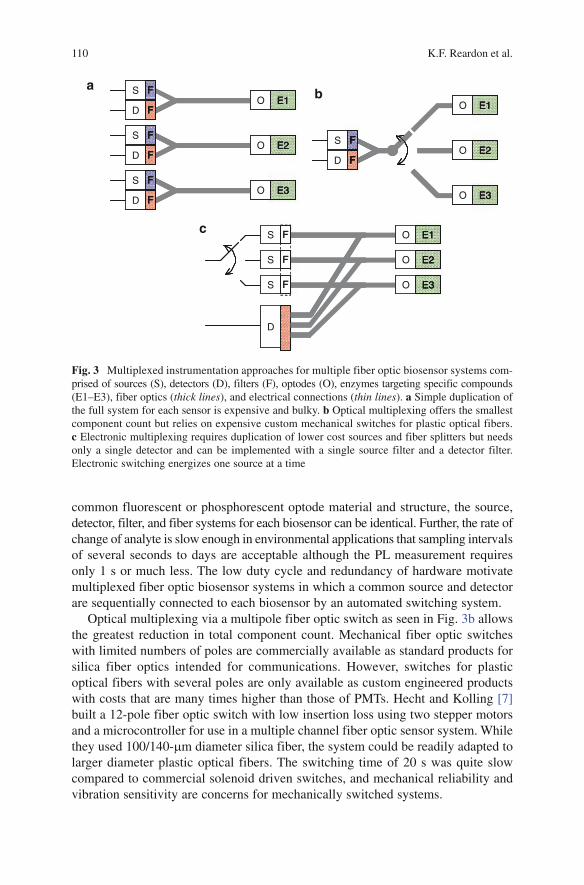
110 K.F. Reardon et al.
common fluorescent or phosphorescent optode material and structure, the source, detector, filter, and fiber systems for each biosensor can be identical. Further, the rate of change of analyte is slow enough in environmental applications that sampling intervals of several seconds to days are acceptable although the PL measurement requires only 1 s or much less. The low duty cycle and redundancy of hardware motivate multiplexed fiber optic biosensor systems in which a common source and detector are sequentially connected to each biosensor by an automated switching system.
Optical multiplexing via a multipole fiber optic switch as seen in Fig. 3b allows the greatest reduction in total component count. Mechanical fiber optic switches with limited numbers of poles are commercially available as standard products for silica fiber optics intended for communications. However, switches for plastic optical fibers with several poles are only available as custom engineered products with costs that are many times higher than those of PMTs. Hecht and Kolling [7] built a 12-pole fiber optic switch with low insertion loss using two stepper motors and a microcontroller for use in a multiple channel fiber optic sensor system. While they used 100/140-mm diameter silica fiber, the system could be readily adapted to larger diameter plastic optical fibers. The switching time of 20 s was quite slow compared to commercial solenoid driven switches, and mechanical reliability and vibration sensitivity are concerns for mechanically switched systems.
Fig. 3 Multiplexed instrumentation approaches for multiple fiber optic biosensor systems com-prised of sources (S), detectors (D), filters (F), optodes (O), enzymes targeting specific compounds (E1–E3), fiber optics (thick lines), and electrical connections (thin lines). a Simple duplication of the full system for each sensor is expensive and bulky. b Optical multiplexing offers the smallest component count but relies on expensive custom mechanical switches for plastic optical fibers. c Electronic multiplexing requires duplication of lower cost sources and fiber splitters but needs only a single detector and can be implemented with a single source filter and a detector filter. Electronic switching energizes one source at a time
O
O
O
S
D
F
F
S
D
F
F
S
D
F
F
E1
E2
E3
O
O
O
S
D
F
F
E3
E2
E1
ab
O
O
O
D
S F
S F
S F E3
E2
E1c
O
O
O
S
D
F
F
S
D
F
F
S
D
F
F
E1
E2
E3
O
O
O
S
D
F
F
S
D F
S
D
F
F
S
D
F
F
S
D
F
F
S
D
F
F
E1
E2
E3
O
O
O
S
D
F
F
E3
E2
E1
O
O
O
S
D
F
FO
O
O
S
D
F
F
S
D
F
F
E3
E2
E1
O
O
O
D
S F
S F
S F E3
E2
E1O
O
O
D
S FS F
S FS F
S FS F E3
E2
E1
Environmental Applications of Photoluminescence-Based Biosensors 111
An alternative approach in development by the authors is electronic multiplexing according to the scheme shown in Fig. 3c and offers competitive or lower costs and likely more rugged construction than optical multiplexing while avoiding custom fiber switches. In this approach, the source and optical fiber related components are duplicated for each channel, but a single PMT is employed due to its high cost and significant size. One source at a time is electrically energized when a measurement for the corresponding sensor is desired. The emissions from all biosensors are con-tinuously, simultaneously input into the large area PMT through a single filter, but only the optode receiving excitation light produces emission. LED sources are used to minimize the cost of these duplicated components. The rapid activation of LEDs allows electronic switching with sub-millisecond sampling intervals if desired. In order to reduce the use of LED source filters, which are significantly more expensive than the LEDs, a single inline filter can be used in parallel by multiple fibers.
4 Biosensors for Chemical Analytes
4.1 Hydrocarbons and Alcohols
Hydrocarbons are the most common group of contaminants found in soil and water, released through the activities associated with petroleum refining and fuel storage and transport. Alcohols are not normally considered to be environmental contami-nants, but ethanol emissions from bakeries may be problematic. Furthermore, with the increased production and use of ethanol and perhaps butanol as biofuels, there is a greater chance that these chemicals will be released into the environment.
Two primary sensing concepts have been used to develop optical biosensors for hydrocarbons and alcohols: enzymatic oxidation with measurement of oxygen consumption, and induction-based detection. The enzyme-based biosensors have primarily been developed for ethanol and use the well known alcohol oxidase, which catalyzes the reaction of ethanol and oxygen to form acetaldehyde and hydrogen peroxide. While electrochemical transducers are frequently used in ethanol biosensors [8], some reports of optical transduction have been published. Mitsubayashi et al. described an optical biosensor in which alcohol oxidase was immobilized on the tip of a fiber optic oxygen sensor that used a photoluminescent ruthenium com-plex [9]. This biosensor was found to detect for ethanol in aqueous solutions in the range 0.5–9 mM and was also effective in gaseous samples with ethanol concentra-tions from 0.7 to 50 ppm. Wen et al. later described a similar system and achieved a lower detection limit in aqueous solution (30 mM), although their biosensor used an oxygen electrode [10]. Another group used coimmobilized alcohol oxidase and horseradish peroxidase, immobilized on an optical oxygen sensor, to measure methanol in n-hexane in the range 2–90 mM [11].
It would be of great interest to develop similar biosensors for the detection of hydrocarbons, and indeed enzymes exist that catalyze the reaction of oxygen with many different hydrocarbons. However, these mono- and dioxygenases also require

112 K.F. Reardon et al.
NAD(P)H as a cofactor, and thus can only be used in whole cells for short periods. A demonstration of this concept was described by Thavarungkul et al., who placed alginate-immobilized Pseudomonas cepacia cells in a flow cell near an oxygen electrode [12]. Detection of various aromatic compounds at approximately 1 mM was achieved. Rella et al. developed a more integrated system by immobilizing phenol-oxidizing Bacillus stearothermophilus in a hydroxyethyl methacrylate membrane that was coupled to an oxygen electrode [13]. Their biosensor responded to phenol, catechol, and related compounds, which is indicative of the moderate specificity of the oxygenase enzymes expressed by these cells. More recently, our group has demonstrated this concept as optical biosensors for the measurement of toluene using whole cells expressing toluene o-monooxygenase and an optical oxygen sensor. A detection limit of 0.3 mg L−1 was achieved, but the useful lifetime of the biosensors was very limited owing to the requirement for NADH [14].
Antibodies are commonly used in bioassay systems to accommodate the addition of reagents that are required in most sensing concepts to detect the binding of an antigen. Vo-Dinh et al. avoided this requirement by taking advantage of the natural fluorescence characteristics of benzo(a)pyrene [15]. Anti-BaP antibodies were immobilized on the tip of a biosensor and the binding of BaP was detected as fluo-rescence in response to excitation from a helium–cadmium laser. The system was very sensitive (LOD < 250 ng L−1) with a specificity that depended on the antibody. However, the sensing concept is restricted to analytes that are photoluminescentIn addition to enzymes and antibodies, a third biosensing principle is that of
induction. In this scenario, illustrated in Fig. 4, the analyte of interest induces transcription of an operon, typically by binding to a transcriptional activator that then binds to the promoter region, activating transcription [16, 17]. The transcriptional event is detected by fusing genes for a reporter protein behind the inducible promoter. While genes for a variety of reporter proteins have been used, those best suited for optical biosensors are those encoding autofluorescent proteins (often green fluorescent protein, gfp, but also red fluorescent protein, dsred), bacterial
Fig. 4 Schematic depiction of induction biosensor concept. The analyte of interest (triangle) binds to a transcriptional activator and the complex activates transcription at the inducible promoter (P), leading to the synthesis of the reporter protein

Environmental Applications of Photoluminescence-Based Biosensors 113
luciferase (the luxCDABE cassette, when the enzymes for synthesis of the reaction substrate are included), and firefly luciferase (lucFF). Several excellent reviews are available on the use of these reporter proteins in biosensors and bioassays, including their relative advantages and disadvantages [16, 18]. The first report of the applica-tion of the induction biosensing approach came from the Sayler group, who con-structed a biosensor for naphthalene and salicylate [19]. This biosensor was based on the reporter bacterium Pseudomonas fluorescens HK44, containing plasmid pUTK21 with the luxDCABE cassette fused with the nahG gene and under control of the P
sal promoter, which is regulated by the nahR gene product [20]. This reporter
strain was immobilized onto the surface of a light guide, and the resulting biosensor produced light in response to both naphthalene and salicylate. Detection of 1.5 mg L−1 naphthalene was reported, and other measurements of real pollutant mixtures were obtained. However, it was necessary to supply the biosensors with growth medium to maintain the ability of the cells to perform the necessary transcription and translation, and the influence of the oxygen level and other param-eters was noted. This induction-based biosensing concept has also been used to con-struct biosensors for toluene, styrene, benzene, and other chemicals (Table 1). While the sensing concept has the advantage of being very general (as long as the appro-priate promoter and transcriptional activator can be identified), there are also the disadvantages of maintaining cell viability and of relatively low specificity. (Somewhat confusingly, the genetically modified cells are themselves often referred to as biosensors.) In addition to the application of induction-based biosensors for the determination of aqueous chemical concentrations, there have been reports of their use for assessing bioavailability enhancement from soils by surfactants [23, 32], illustrating the advantages of in situ measurements over the typical approach of laboratory-based methods involving organic solvent extraction.
4.2 Halogenated Organics
Halogenated organic chemicals form a diverse group of frequent interest for environmental monitoring. This group includes halogenated solvents (e.g., trichlo-roethene and tetrachloroethene) used in very large amounts each year, halogenated aromatics that are products or intermediates in industrial chemical processes (e.g., polychlorinated biphenyls (PCBs)), and halogenated aromatics and heterocyclic compounds that are formed as byproducts of combustion or chemical processing (e.g., dioxin). Many pesticides, such as lindane, are also halogenated.
Each of the three main optical biosensing strategies described in the previous sec-tion is also represented among the reports for biosensors for halogenated organics. The enzymatic approach has been described by several groups, most of which relied upon one or more enzymes from the class of hydrolytic haloalkane dehalogenases for detection of halogenated haloalkanes [33–37]. While most of these reports describe bioassays, and only one describes an optical biosensor, there is a common theme regarding the biocomponent. An optical biosensor for the measurement of 1,2-dichlo-roethane (DCA) in aqueous samples was published by our group [33]. This sensor

Tabl
e 1
Indu
ctio
n-ba
sed
bioa
ssay
s fo
r ch
emic
al a
naly
tes
Ana
lyte
Indu
ctio
n sy
stem
Rep
orte
rC
omm
ents
Ref
eren
ce
Tolu
ene
and
othe
r ar
omat
ics
xylR
and
Pu
of T
OL
pla
smid
of
Pse
udom
onas
put
ida
mt-
2lu
cFF
Res
pond
s to
xyl
enes
and
chl
orin
ated
tolu
enes
m
ore
stro
ngly
than
to to
luen
eL
OD
of
10–2
0 mM
tolu
ene
(in
cell
susp
ensi
on)
2–3
h fo
r fu
ll si
gnal
Lin
ear
resp
onse
in th
e ra
nge
5–20
mg
L−
1 to
luen
eTe
sted
with
con
tam
inat
ed g
roun
d w
ater
with
go
od c
orre
latio
n to
GC
-MS
valu
es
[21]
Benzene, toluene, ethylbenzene,
xyle
nes
xylR
and
Pu
of T
OL
pla
smid
of
Pse
udom
onas
put
ida
mt-
2gf
p, l
uxC
DA
BE
Res
pond
s to
xyl
enes
and
nap
htha
lene
mor
e
stro
ngly
than
tolu
ene
Lum
ines
cenc
e re
port
er m
ore
sens
itive
but
GFP
si
gnal
mor
e st
able
with
tim
e2–
3 h
for
full
sign
alL
ow li
near
ity o
f re
spon
seTe
sted
with
con
tam
inat
ed g
roun
d w
ater
but
low
co
rrel
atio
n w
ith G
C-M
S va
lues
[22]
Phen
anth
rene
phnS
put
ativ
e pr
omot
er/o
pera
tor
regi
on
(Bur
khol
deri
a sp
. str
ain
RP0
37)
gfp
Res
pond
s to
nap
htha
lene
mor
e st
rong
ly th
an
phen
anth
rene
; als
o re
spon
ds to
ant
hrac
ene
2 h
for
full
sign
alL
OD
not
det
erm
ined
[23]
Styr
ene
Pst
y of
Pse
udom
onas
sp.
str
ain
Y2
lacZ
Res
pond
s to
sty
rene
, tol
uene
, and
epo
xyst
yren
e1
h fo
r fu
ll si
gnal
LO
D n
ot d
eter
min
ed
[24]
2-H
aloa
cids
2-H
aloa
cid
deha
loge
nase
pro
mot
er o
f P
seud
omon
as s
p. s
trai
n 11
3lu
xCD
AB
ER
espo
nds
to p
ropi
onic
aci
d an
d 2-
chlo
ro-
and
2-br
omop
ropi
nic
acid
; oth
erw
ise,
hig
h
spec
ific
ityL
inea
r re
spon
se o
ver
rang
e 0.
5–2
mg
L−
1
chlo
ropr
opio
nate
but
hig
h si
gnal
var
iabi
lity
6 h
for
full
sign
al
[25]
Chl
orin
ated
phe
nols
P dmp
and
mut
ated
Dm
pR f
rom
the
dmp
oper
on o
f P
seud
omon
as s
p. s
trai
n C
F600
lacZ
Res
pond
s to
phe
nol a
nd m
ono-
and
di
-chl
oro-
, met
hyl,
and
nitr
ophe
nols
Res
pons
e de
pend
s on
Dm
pR m
utan
t use
dD
etec
tion
of 1
3 mg
L−
1 2-
chlo
roph
enol
[26]

2,3,7,8-Tetrachlorodibenzo
-p-d
ioxi
n (T
CD
D)
Dio
xin-
resp
onsi
ve e
lem
ent (
DR
E)
seap
Use
s m
urin
e he
pato
ma
cells
LO
D =
100
fM
TC
DD
Res
pond
ed to
oth
er D
RE
act
ivat
ors
[27]
Mer
cury
Prom
oter
of
mer
R o
f tr
ansp
oson
21
luxC
DA
BE
LO
D =
100
ng
L−
1 H
g2+ (
scin
tilla
tion
coun
ter)
1 h
for
full
sign
alD
etec
tion
in s
pike
d na
tura
l wat
ers
corr
elat
ed w
ell
to s
tand
ard
met
hods
Sele
ctiv
ity n
ot d
eter
min
ed
[28]
Cad
miu
m, l
ead
Prom
oter
of
cad
of S
taph
yloc
occu
s
aure
us p
lasm
id p
I258
lucF
FM
ost s
ensi
tive
to c
adm
ium
but
als
o re
spon
ded
to antimony, zinc, tin, and lead.
2 h
for
mea
sure
d si
gnal
LO
D =
370
ng
L−
1 C
d
[29]
Ura
nium
Prom
oter
of
urcA
of
Cau
loba
cter
cre
s-ce
ntus
gfp
LO
D =
120
mg
L−
1 ur
aniu
mG
ood
sele
ctiv
ity w
ith lo
w s
ensi
tivity
for
lead
, ca
dmiu
m, a
nd c
hrom
ium
.3
h fo
r fu
ll si
gnal
[30]
Gen
otox
ic c
ompo
unds
Prom
oter
of
cda
of E
sche
rich
ia c
oli
gfp
LO
D =
24 mg
L−
1 N
-met
hyl-
N-n
itro-
N-
nitr
osog
uani
dine
(M
NN
G)
Res
pond
s to
MN
NG
, mito
myc
in C
, nal
idix
ic a
cid,
ot
hers
Lin
ear
resp
onse
ran
ge f
or M
NN
G
[31]
Rep
orte
rs: l
ucF
F =
fir
efly
luci
fera
se; l
uxC
DA
BE
= b
acte
rial
luci
fera
se; g
fp =
gre
en f
luor
esce
nt p
rote
in; l
acZ
= b
-gal
acto
sida
se; s
eap
= s
ecre
ted
alka
line
phos
phat
ase
LO
D =
lim
it of
det
ectio
n
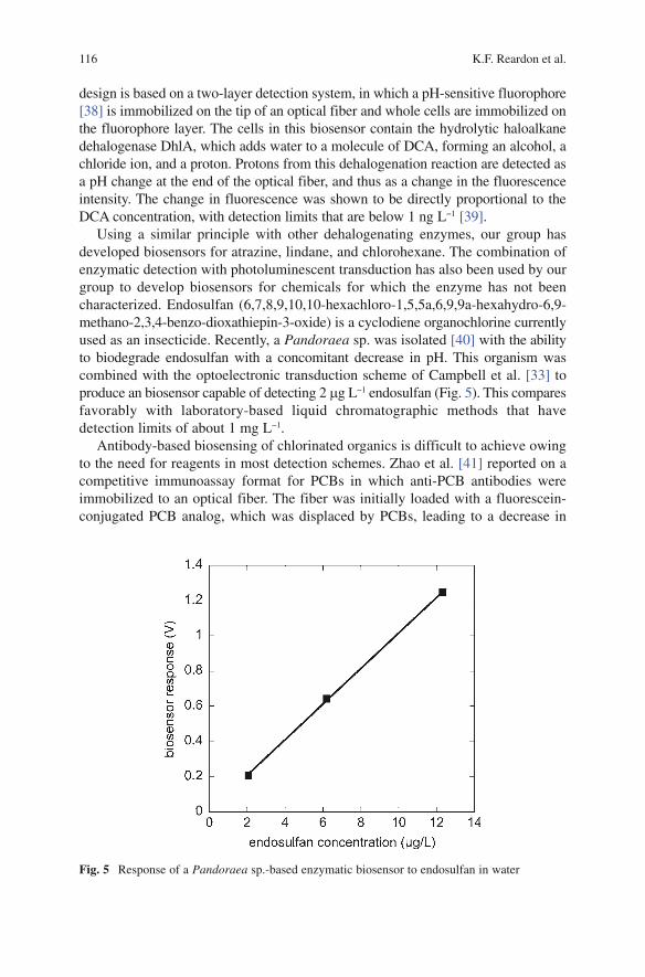
116 K.F. Reardon et al.
design is based on a two-layer detection system, in which a pH-sensitive fluorophore [38] is immobilized on the tip of an optical fiber and whole cells are immobilized on the fluorophore layer. The cells in this biosensor contain the hydrolytic haloalkane dehalogenase DhlA, which adds water to a molecule of DCA, forming an alcohol, a chloride ion, and a proton. Protons from this dehalogenation reaction are detected as a pH change at the end of the optical fiber, and thus as a change in the fluorescence intensity. The change in fluorescence was shown to be directly proportional to the DCA concentration, with detection limits that are below 1 ng L−1 [39].Using a similar principle with other dehalogenating enzymes, our group has
developed biosensors for atrazine, lindane, and chlorohexane. The combination of enzymatic detection with photoluminescent transduction has also been used by our group to develop biosensors for chemicals for which the enzyme has not been characterized. Endosulfan (6,7,8,9,10,10-hexachloro-1,5,5a,6,9,9a-hexahydro-6,9-methano-2,3,4-benzo-dioxathiepin-3-oxide) is a cyclodiene organochlorine currently used as an insecticide. Recently, a Pandoraea sp. was isolated [40] with the ability to biodegrade endosulfan with a concomitant decrease in pH. This organism was combined with the optoelectronic transduction scheme of Campbell et al. [33] to produce an biosensor capable of detecting 2 mg L−1 endosulfan (Fig. 5). This compares favorably with laboratory-based liquid chromatographic methods that have detection limits of about 1 mg L−1.
Antibody-based biosensing of chlorinated organics is difficult to achieve owing to the need for reagents in most detection schemes. Zhao et al. [41] reported on a competitive immunoassay format for PCBs in which anti-PCB antibodies were immobilized to an optical fiber. The fiber was initially loaded with a fluorescein-conjugated PCB analog, which was displaced by PCBs, leading to a decrease in
Fig. 5 Response of a Pandoraea sp.-based enzymatic biosensor to endosulfan in water

Environmental Applications of Photoluminescence-Based Biosensors 117
measured fluorescence. The response time was short (seconds to minutes), and thus it is possible that this assay could be implemented in a way that provides near real-time measurements.
Induction-based biosensing has been reported for halogenated organic acids, chlorophenols, chlorocatechols, and dioxins, among others (Table 1). Of particular note is a study by Kasai et al. [27] on the use of a nonbacterial host for the inducible gene. These researchers used a murine hepatoma cell line to host a plasmid containing a dioxin-responsive element fused to a viral promoter upstream of a reporter gene. In an assay mode, the reported limit of detection was 100 fM of dioxin. Although the reporter protein used in their study was not one that could be used with a photo-luminescence transducer, it would be straightforward to make this conversion and create an optical biosensor from this sensing construct (albeit with the usual limits for induction biosensors of maintaining cell viability).
4.3 Nitro-, Phospho-, Sulfo-, and Other Substituted Organics
Many different substituted aromatic and aliphatic organic chemicals are of impor-tance for environmental monitoring. For example, organophosphates have been used as pesticides (e.g., methyl parathion) and as nerve agents (sarin). Sulfonated organ-ics are used in the dye industry (e.g., methylene blue). Organic molecules containing nitrogen moieties are also used in the dye industry (e.g., Acid Orange 7), as explosives (e.g., trinitrotoluene), and as precursors for organic syntheses (e.g., nitrobenzene for aniline). Despite the very large scale at which these chemicals are used (and the significant toxicity of many of them), there are relatively few reports of biosensors developed for their detection, even when bioassays are also considered.
In principle, an optical biosensor for a particular substituted organic could be developed using an enzyme, antibody, or induction sensing scheme. In the case of an enzyme-based biosensor, it would be necessary to find an enzyme that catalyzes a reaction with the analyte to produce or consume a species that could be detected optically, either directly or indirectly. One example is the use of organophosphate hydrolase (OPH), which hydrolyzes organophosphates to produce protons and cleavage products, some of which are chromophoric (e.g., p-nitrophenol from parathions). The group of Mulchandani and Chen has generated a variety of biosensor designs based on OPH, two of which can be adapted for photoluminescence-based biosensing. The first is the detection of the protons produced in the reaction. Originally, this was done by immobilizing OPH or OPH-expressing bacteria on a pH electrode [42]; our group has subsequently used a pH optode to produce an optical biosensor for paraoxon with a detection limit below 1 ng L−1 (unpublished results). The second OPH-based biosensor concept involves the use of aerobic microorganisms that consume the products of the OPH reaction and measurement of the corresponding decrease in oxygen. Although the Mulchandani and Chen group used oxygen electrodes to demonstrate this concept [43, 44], an oxygen optode could also be used to create a photoluminescence-based biosensor.
118 K.F. Reardon et al.
As noted previously, antibody-based optical detection methods for substituted organics nearly always rely on the addition of a reagent to detect the antibody–antigen binding and are thus assays instead of biosensors. Semicontinuous measurements could be performed if the detection system is incorporated into a flow injection analysis system [45], although the ability to obtain in situ measurements would still be limited. Some reports of antibody-based photoluminescence assays have been published. For example, an assay for trinitrotoluene (TNT) was developed based on the competition between TNT in the sample and fluorophore-labeled trinitrobenzene that was added [46]. The two nitroaromatics competed for antibody immobilized on an optical fiber, with higher TNT concentrations corresponding to lower fluorescence measurements. A detection limit for TNT of 10 mg L−1 was obtained.
The development of induction-based biosensors for substituted organics depends upon the ability to identify transcription regulatory elements that are responsive to the analyte of interest. Two approaches to this challenge have been reported. In one case, DNA microarrays were used to identify genes in Saccharomyces cerevisiae that were induced in the presence of the organophosphate paraoxon as well as those associated with the hydrolysis of paraoxon [47]. The promoters of highly responsive genes were fused to genes encoding either red (yDSRed) or green (yEGFP) fluorescent protein to create yeast strains that could be used as biocomponents in photoluminescence-based biosensors. The second approach was to use mutation-prone PCR and DNA shuffling to create variants of the toluene-responsive XylR regulator that were instead responsive to mono-, di-, and tri-nitrotoluenes [48]. These two reports demonstrate that the desired responsive elements can be identified through genomic searches or through modification of known regulators.
4.4 Metals and Other Inorganics
Although organic chemicals are the most common environmental contaminants, the detection of inorganic compounds is also of importance. Heavy metal contamination through metal plating operations (mainly chromate) and from acid mine drainage (e.g., copper, cadmium, mercury) are of concern in many areas around the world. Arsenic and selenium are found in high levels in lakes and groundwater as a result of natural and human factors. Furthermore, nitrate and phosphate contamination of waters may occur through over-application of fertilizers or as runoff from cattle feedlot operations.Enzyme-based biosensors for such inorganics are limited by the ability to
identify reactions with reactants or products that are detectable with a photolumi-nescence scheme, and antibodies that are specific for such small molecules are difficult to obtain. Thus, nearly all reports of biosensors for this group of contaminants rely on the induction approach. This is facilitated by a large body of research on mechanisms of metal resistance in microorganisms, which has revealed numerous metal-responsive genetic elements [49–51]. Many such biosensor constructs have been developed for mercury. For example, Selifonova et al. [28] used portions of

Environmental Applications of Photoluminescence-Based Biosensors 119
the mercury resistance operon of transposon 21 fused to the luxCDABE cassette to create E. coli reporter strains for Hg2+. A scintillation counter was used to detect luminescence and detection as low as 1 nM was reported. Harkins et al. [52] compared nine such Hg2+ reporter strains constructed with different regulatory ele-ments, reporter proteins, and host organisms. Similar bacterial reporter strains have been developed for cadmium [29, 53], lead [54], copper [55], uranium [30], nickel [56], arsenic [57, 58], and other metals (Table 1).
An interesting binding-based biosensor for copper was developed by Zeng et al. [59]. Carbonic anhydrase was labeled with a fluorophore in such a way that the binding of Cu2+ to the protein resulted in changes in fluorescence intensity and lifetime. Detection of 0.1 pM Cu2+ in seawater was reported, and the authors note that similar sensors for other cations could be developed using variants of carbonic anhydrase.
4.5 Chemical Mixtures
In the environment, contaminants are most often found in mixtures. This applies to soil and ground water at hazardous waste sites, as well as waste waters from industrial and municipal sources. Common examples of chemical mixtures that often become pollutants include gasoline and other petroleum fuels, pesticides, and wood-treating substances. Landfill leachates are complex mixtures that contaminate ground water supplies around the world. Pollutant mixtures may contain only organic chemicals or may also include inorganics, heavy metals, or radionuclides. The presence of mixtures of analytes poses at least two challenges for environmental measurements. The first is the ability of an analytical method to detect a specific chemical of interest in a background of other chemicals, some of which may have similar structures. This is the issue of selectivity and is an important characteristic of any analytical method. The second challenge for analysis of chemical mixtures is the goal of obtaining information on the entire mixture, the chemical composition of which is normally not known. In this section, we consider biosensor approaches to this problem of general mixture analysis.The traditional methods used to characterize chemical mixtures in wastewaters
are chemical oxygen demand and biological oxygen demand (BOD). The latter method is based on measurement of the oxygen consumed in a certain period by a microbial culture growing on organic chemicals in the sample. Numerous groups have adapted this approach to construct optical BOD sensors. These sensors involve a microbial culture immobilized on an oxygen optode. Thus, Chee et al. [60] used a pure culture of Pseudomonas putida to construct an optical BOD biosensor. When calibrated with an artificial wastewater of known composition, this biosensor yielded measurements that correlated well with the standard method over a low BOD range (1–10 mg L−1 BOD). The response time was 15 min, providing a considerable throughput advantage over the standard 5-day measurement time. The choice of microbial culture is important for any BOD analysis since a wide range of organic chemicals may be present, and thus other groups have evaluated
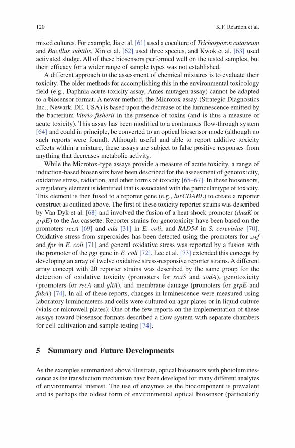
120 K.F. Reardon et al.
mixed cultures. For example, Jia et al. [61] used a coculture of Trichosporon cutaneum and Bacillus subtilis, Xin et al. [62] used three species, and Kwok et al. [63] used activated sludge. All of these biosensors performed well on the tested samples, but their efficacy for a wider range of sample types was not established.
A different approach to the assessment of chemical mixtures is to evaluate their toxicity. The older methods for accomplishing this in the environmental toxicology field (e.g., Daphnia acute toxicity assay, Ames mutagen assay) cannot be adapted to a biosensor format. A newer method, the Microtox assay (Strategic Diagnostics Inc., Newark, DE, USA) is based upon the decrease of the luminescence emitted by the bacterium Vibrio fisherii in the presence of toxins (and is thus a measure of acute toxicity). This assay has been modified to a continuous flow-through system [64] and could in principle, be converted to an optical biosensor mode (although no such reports were found). Although useful and able to report additive toxicity effects within a mixture, these assays are subject to false positive responses from anything that decreases metabolic activity.
While the Microtox-type assays provide a measure of acute toxicity, a range of induction-based biosensors have been described for the assessment of genotoxicity, oxidative stress, radiation, and other forms of toxicity [65–67]. In these biosensors, a regulatory element is identified that is associated with the particular type of toxicity. This element is then fused to a reporter gene (e.g., luxCDABE) to create a reporter construct as outlined above. The first of these toxicity reporter strains was described by Van Dyk et al. [68] and involved the fusion of a heat shock promoter (dnaK or grpE) to the lux cassette. Reporter strains for genotoxicity have been based on the promoters recA [69] and cda [31] in E. coli, and RAD54 in S. cerevisiae [70]. Oxidative stress from superoxides has been detected using the promoters for zwf and fpr in E. coli [71] and general oxidative stress was reported by a fusion with the promoter of the pgi gene in E. coli [72]. Lee et al. [73] extended this concept by developing an array of twelve oxidative stress-responsive reporter strains. A different array concept with 20 reporter strains was described by the same group for the detection of oxidative toxicity (promoters for soxS and sodA), genotoxicity (promoters for recA and gltA), and membrane damage (promoters for grpE and fabA) [74]. In all of these reports, changes in luminescence were measured using laboratory luminometers and cells were cultured on agar plates or in liquid culture (vials or microwell plates). One of the few reports on the implementation of these assays toward biosensor formats described a flow system with separate chambers for cell cultivation and sample testing [74].
5 Summary and Future Developments
As the examples summarized above illustrate, optical biosensors with photolumines-cence as the transduction mechanism have been developed for many different analytes of environmental interest. The use of enzymes as the biocomponent is prevalent and is perhaps the oldest form of environmental optical biosensor (particularly
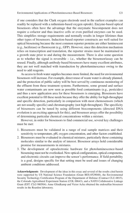
Environmental Applications of Photoluminescence-Based Biosensors 121
if one considers that the Clark oxygen electrode used in the earliest examples can readily be replaced with a ruthenium-based oxygen optode). Enzyme-based optical biosensors often have the advantage that the enzymatic biocomponent does not require a cofactor and thus inactive cells or even purified enzymes can be used. This simplifies storage requirements and normally results in longer lifetimes than other types of biosensors. Induction-based reporter constructs are well suited for optical biosensing because the most common reporter proteins are either luminescent (e.g., luciferase) or fluorescent (e.g., GFP). However, since this detection mechanism relies on transcription and translation, the reporter strains must be maintained in a growth state prior to and during the measurement. There is also some question as to whether the signal is reversible – i.e., whether the biosensor/assay can be reused. Finally, although antibody-based biosensors have many excellent attributes, they are not well matched with transduction by photoluminescence owing to the need to add reagents.
As access to fresh water supplies becomes more limited, the need for environmental biosensors will increase. For example, direct reuse of waste water is already planned, and the protection of public safety will be best served by continuous monitoring of the effluent from these treatment systems. Furthermore, some ground and surface water contaminants are now seen as possible food contaminants (e.g., pesticides) and thus a new application area for these biosensors is emerging. Biosensors have excellent potential to fill these needs because they offer the ability for high-throughput and specific detection, particularly in comparison with most chemosensors (which are not usually specific) and chromatography (not high throughput). The specificity of biosensors can be tuned by using different biocomponents (directed DNA evolution is an exciting approach for this), and biosensor arrays offer the possibility of determining particular chemical concentrations within a mixture.
However, in order for biosensors to find commercial use, several key challenges must be met:
1. Biosensors must be validated in a range of real sample matrices and their sensitivity to temperature, pH, oxygen concentration, and other factors established.
2. Biosensors must be evaluated in chemical mixtures, particularly those containing molecules similar to the analyte of interest. Biosensor arrays hold considerable promise for measurements in mixtures.
3. The development of optoelectronic hardware for photoluminescence-based biosensing must not be overlooked. New optical configurations, optical components, and electronic circuits can improve the sensor’s performance. If field portability is a goal, designs specific for that setting must be used and issues of changing ambient conditions addressed.
Acknowledgments Development of the ideas in this essay and several of the results cited herein were supported by US National Science Foundation (Grant BES-0529048), the Environmental Security Technology Certification Program of the Department of Defense (Contract CLU-0015), the Colorado Agricultural Experiment Station (COL 00643), and a NATO Collaborative Linkage Grant (EST. CLG 980504). Anne Glindkamp and Victor Acha obtained the endosulfan biosensor results in the Reardon laboratory.

122 K.F. Reardon et al.
References
1. Fähnrich K, Pravda M, Guilbault GG (2003) Biosens Bioelectron 18(1):73 2. Salmain M, Fischer-Durand N, Pradier CM (2008) Anal Biochem 373(1):61 3. Dennison MJ, Turner APF (1995) Biotechnol Adv 13(1):1 4. Rogers KR (1995) Biosens Bioelectron 10(6/7):533 5. Pieper S, Mestas S, Lear K, Zhong Z, Reardon K (2008) Appl Phys Lett 92(8):081915 6. Agishev R, Gross B, Moshary F, Gilerson A, Ahmed S (2006) Optic Laser Eng 44(8):779 7. Hecht H, Kolling M (2001) Sens Actuators B Chem 81(1):128 8. Azevedo AM, Prazeres DMF, Cabral JMS, Fonseca LP (2005) Biosens Bioelectron
21(2):235 9. Mitsubayashi K, Matsunaga H, Nishio G, Toda S, Nakanishi Y (2005) Biosens Bioelectron
20(8):157310. Wen G, Zhang Y, Shuang S, Dong C, Choi M (2007) Biosens Bioelectron 23(1):12111. Wu X, Choi M, Chen C, Wu X (2007) Biosens Bioelectron 22(7):133712. Thavarungkul P, Hakanson H, Mattiasson B (1991) Anal Chim Acta 249(1):1713. Rella R, Ferrara D, Barison G, Doretti L, Lora S (1996) Biotechnol Appl Biochem 24:8314. Zhong Z, Fritzsche M, Pieper S, Wood TK, Lear KL, Dandy DS, Reardon KF (2008)15. Vo-Dinh T, Tromberg BJ, Griffin GD, Ambrose KR, Sepaniak MJ, Gardenhire EM (1987)
Appl Spectrosc 41(5):73516. Harms H, Wells MC, van der Meer JR (2006) Appl Microbiol Biotechnol 70(3):27317. Marques S, Arandaolmedo I, Ramos J (2006) Curr Opin Biotechnol 17(1):5018. Paitan Y, Biran D, Biran I, Shechter N, Babai R, Rishpon J, Ron EZ (2003) Biotechnol Adv
22(1/2):2719. Heitzer A, Malachowsky K, Thonnard JE, Bienkowski PR, White DC, Sayler GS (1994)
Appl Environ Microbiol 60(5):148720. Burlage RS, Sayler GS, Larimer F (1990) J Bacteriol 172(9):474921. Willardson BM, Wilkins JF, Rand TA, Schupp JM, Hill KK, Keim P, Jackson PJ (1998)
Appl Environ Microbiol 64(3):100622. Li Y, Li F, Ho C, Liao VH (2008) Environ Pollut 152(1):12323. Tecon R, Wells M, van der Meer JR (2006) Environ Microbiol 8(4):69724. Alonso S, Navarro-Llorens JM, Tormo A, Perera J (2003) J Biotechnol 102(3):30125. Tauber M, Rosen R, Belkin S (2001) Talanta 55(5):95926. Wise AA, Kuske CR (2000) Appl Environ Microbiol 66(1):16327. Kasai A, Hiramatsu N, Meng Y, Yao J, Takeda M, Maeda S, Kitamura M (2004) Anal Biochem
335(1):7328. Selifonova O, Burlage R, Barkay T (1993) Appl Environ Microbiol 59(9):308329. Tauriainen S, Karp M, Chang W, Virta M (1998) Biosens Bioelectron 13(9):93130. Hillson N, Hu P, Andersen G, Shapiro L (2007) Appl Environ Microbiol 73(23):761531. Norman A, Hansen LH, Sorensen SJ (2005) Appl Environ Microbiol 71(5):233832. Keane A, Lau PCK, Ghoshal S (2008) Biotechnol Bioeng 99(1):8633. Campbell DW, Müller C, Reardon KF (2006) Biotechnol Lett 28(12):88334. Henrysson T, Mattiasson B (1993) Biodegradation 4(2):10135. Hutter W, Peter J, Swoboda H, Hampel W, Rosenberg E, Kramer D, Kellner R (1995)
Anal Chim Acta 306(2/3):23736. Peter J, Hutter W, Stöllnberger W, Hampel W (1996) Biosens Bioelectron 11(12):121537. Peter J, Hutter W, Stöllnberger W, Karner F, Hampel W (1997) Anal Chem 69:207738. Zhujun Z, Zhang Y, Wangbai M, Russell R, Shakhsher ZM, Grant CL, Seitz WR, Sundberg DC
(1989) Anal Chem 61(3):20239. Acha V, Damborsky J, Reardon KF (2008)40. Siddique T, Okeke BC, Arshad M, Frankenberger WT (2003) J Agric Food Chem 51(27):801541. Zhao CQ, Anis NA, Rogers KR, Kline RH, Wright J, Eldefrawi AT, Eldefrawi ME (1995) J
Agric Food Chem 43(8):2308

Environmental Applications of Photoluminescence-Based Biosensors 123
42. Mulchandani A, Mulchandani P, Chen W (1998) Field Anal Chem Technol 2(6):363–36743. Lei Y, Mulchandani P, Chen W, Mulchandani A (2006) Sensors 6(4):46644. Mulchandani P, Chen W, Mulchandani A (2006) Anal Chim Acta 568(1–2):21745. Ruzicka J, Hansen EH (1988) Flow injection analysis, 2nd edn. Wiley, Weinheim, pp 52846. Shriver-Lake L, Breslin KA, Charles PT, Conrad DW, Golden JP, Ligler FS (1995) Anal
Chem 67(14):243147. Schofield D, Westwater C, Barth J, Dinovo A (2007) Appl Microbiol Biotechnol 76(6):138348. Garmendia J, De Las Heras A, Galvão T, De Lorenzo V (2008) Microb Biotech 1(3):23649. Collard JM, Corbisier P, Diels L, Dong Q, Jeanthon C, Mergeay M, Taghavi S, van der Lelie D, Wilmotte A, Wuertz S (1994) FEMS Microbiol Rev 14(4):405
50. Silver S (1996) Gene 179(1):951. Verma N, Singh M (2005) BioMetals 18(2):12152. Harkins M, Porter AJ, Paton GI (2004) J Appl Microbiol 97(6):119253. Park J, Sohn M, Oh D, Kwon O, Rhee S, Hur C, Lee S, Gellissen G, Kang H (2007) Appl Environ
Microbiol 73(19):599054. Ivask A, Francois M, Kahru A, Dubourguier HC, Virta M, Douay F (2004) Chemosphere
55(2):14755. Stoyanov JV, Magnani D, Solioz M (2003) FEBS Lett 546(2/3):39156. Tibazarwa C, Corbisier P, Mench M, Bossus A, Solda P, Mergeay M, Wyns L, van der Lelie D
(2001) Environ Pollut 113(1):1957. Ramanathan S, Shi W, Rosen BP, Daunert S (1997) Anal Chem 69(16):338058. Tauriainen S, Karp M, Chang W, Virta M (1997) Appl Environ Microbiol 60:1414–142059. Zeng HH, Thompson RB, Maliwal BP, Fones GR, Moffett JW, Fierke CA (2003) Anal Chem
75(24):680760. Chee GJ, Nomura Y, Ikebukuro K, Karube I (2000) Biosens Bioelectron 15(7/8):37161. Jia JB, Tang MY, Chen X, Li Q, Dong SJ (2003) Biosens Bioelectron 18(8):102362. Xin LL, Wang XD, Guo GM, Wang XR, Chen X (2007) Meas Sci Technol 18(9):287863. Kwok NY, Dong SJ, Lo WH, Wong KY (2005) Sens Actuators B Chem 110(2):28964. Stolper P, Fabel S, Weller M, Knopp D, Niessner R (2008) Anal Bioanal Chem 390(4):118165. Gu M, Mitchell R, Kim B (2004) Adv Biochem Eng Biotechnol 87:26966. Sørensen SJ, Burmølle M, Hansen LH (2006) Curr Opin Biotechnol 17(1):1167. Vollmer AC, Van Dyk TK (2004) Adv Microb Physiol 49:13168. Van Dyk TK, Majarian WR, Konstantinov KB, Young RM, Dhurjati PS, LaRossa RA (1994)
Appl Environ Microbiol 60(5):141469. Bartolome AJ, Ulber R, Scheper T, Sagi E, Belkin S (2003) Sens Actuators B Chem 89(1/2):2770. Knight AW, Goddard NJ, Fielden PR, Barker MG, Billinton N, Walmsley RM (1999) Meas
Sci Technol 10(3):21171. Niazi JH, Kim BC, Gu MB (2007) Appl Microbiol Biotechnol 74(6):127672. Niazi J, Kim B, Ahn JM, Gu M (2008) Biosens Bioelectron 24(4):67073. Lee J, Youn C, Kim B, Gu M (2007) Biosens Bioelectron 22(9/10):222374. Lee J, Mitchell R, Kim B, Cullen D, Gu M (2005) Biosens Bioelectron 21(3):500

Optical Inline Measurement Procedures for Counting and Sizing Cells in Bioprocess Technology
Guido Rudolph, Patrick Lindner, Arne Bluma, Klaus Joeris, Geovanni Martinez, Bernd Hitzmann, and Thomas Scheper
Abstract To observe and control cultivation processes, optical sensors are used increasingly. Important parameters for controlling such processes are cell count, cell size distribution, and the morphology of cells. Among turbidity measurement methods, imaging procedures are applied for determining these process parameters. A disadvantage of most previously developed imaging procedures is that they are only available offline which requires sampling. On the other hand, available imaging inline probes can so far only deliver a limited number of process parameters. This chapter presents new optical procedures for the inline determination of cell count, cell size distribution, and other parameters. In particular, by in situ microscopy an imaging procedure will be described which allows the determination of direct and nondirect cell parameters in real time without sampling.
Keywords Cell size distribution • Focused beam reflectance measurement (FBRM) • In situ microscopy • Inline monitoring • Optical sensors
G. Rudolph, P. Lindner, A. Bluma, B. Hitzmann and T. Scheper () Institut für Technische Chemie, Gottfried Wilhelm Leibniz Universität Hannover, Callinstr. 3, 30167 Hannover, Germany e-mail: [email protected], [email protected], [email protected], [email protected]
K. Joeris Bayer HealthCare, 800 Dwight Way, 94710, Berkeley, CA, USA e-mail: [email protected]
G. Martinez IPCV-LAB, Escuela de Ingeniería Eléctrica, Universidad de Costa Rica, 2060 San José, Costa Rica, USAe-mail: [email protected]
Adv Biochem Engin/Biotechnol (2009) 116: 125–142DOI: 10.1007/10_2009_12© Springer-Verlag Berlin Heidelberg 200Published online: 16 July 2009
9

126 G. Rudolph et al.
1 Introduction
Various pharmaceutical agents and food additives are produced by the cultivation of microorganisms. As efficiency of the bioprocess is only accessible by a sophis-ticated process control, cultivation process data must be collected and analyzed in real time [1]. Moreover, stricter conditions of the FDA (Food and Drug Association) for pharmaceutical industry concerning process documentation imposed by the PAT initiative (process and analytical technology) have increased the demand for inline sensors which are able to monitor and document the production process very accurately.
A disadvantage of most previously developed procedures is that they are only available offline which requires manual sampling, thus representing a contamination risk. After sampling the sample is admitted to the ex situ analysis system with a certain time delay. Thus the measurement result may not correspond to the real state of the process. For this account there is a demand for cultivation sensors which allow a direct inline observation in real time without offline sampling. An approach in this contribution is the development of optical, i.e., imaging techniques.
Imaging procedures for the observation of industrial bioprocesses have been used for years. The observation of processes in which knowledge of concentration and size distribution of suspended cells is important is mostly carried out with either nephelometry or turbidimetry. Nephelometry is based on the measurement of particle light scatter induced in turbid media whereas turbidimetry measures the absorption of light induced by scattering. These techniques are reviewed elsewhere [1–4].
Most turbidity measurement methods have the disadvantage of being available only offline or at line (bypass sensor). Furthermore, most systems only show linear measurement behavior at low particle concentrations. At higher particle concentrations the ratio between increasing light scattering and decreasing trans-mission is no longer proportional and thus the behavior is nonlinear. Only such sensors working with backscattered light also have linear behavior at high particle concentrations. The only commercially available inline system is the FBRM by Mettler Toledo/Lasentec.
Contents
1 Introduction .......................................................................................................................... 1262 Layout and Operation Mode of Different Inline Measurement Techniques ........................ 127
2.1 Focused Beam Reflectance Measurement .................................................................. 1272.2 In situ Microscopy ...................................................................................................... 129
3 New Applications and Developments .................................................................................. 1363.1 Visualization of Morphological Changes.................................................................... 1363.2 Monitoring of Adherent Cells in Microcarrier Culture ............................................... 1373.3 Cell Density Estimation in Three-Dimensional Cell Clusters .................................... 1373.4 Monitoring of Crystallizations .................................................................................... 1393.5 Viability Estimation .................................................................................................... 140
4 Summary .............................................................................................................................. 141References .................................................................................................................................. 141

Optical Inline Measurement Procedures for Counting 127
Due to the fast evolution of CCD-cameras, several offline and inline imaging procedures were developed over the past few years. These measurement techniques allow the direct determination of parameters such as cell concentration or cell size distribution. Established offline systems are the Cedex by Innovatis or the Vi-cell by Beckmann Coulter. These systems take images from a sample and analyzes them with image analysis algorithms in matters of cell density, cell size distribution, and viability.
Currently available imaging inline systems are on the one hand the particle vision and measurement (PVM) by Mettler Toledo/Lasentec and on the other hand the in situ microscope (ISM) by Sartorius. Inline microscopes allow image acquisition directly inside the reactor (in situ), in which the probe is immersed during the whole process. These probes possess either a mechanical or an optical defined sampling zone and analyze the image data with sophisticated image analysis algorithms. Thus information about cell concentration, cell size distribution, and other relevant process parameters are on hand without any delay. Then this information can act as a reliable database for process control.
In the following the state of the art concerning imaging in situ sensors for cell size distribution in biotechnology is reflected. Different optical inline probes are presented with their construction layout, operation mode, and applications. Finally by means of new applications and ongoing developments the strong potential of imaging inline microscopes shall be pointed out.
2 Layout and Operation Mode of Different Inline Measurement Techniques
2.1 Focused Beam Reflectance Measurement
An established inline particle measurement method which bases on the detection of backscattering laser light (180° light scatter) is the patented focused beam reflectance measurement (FBRM) procedure. The method does not measure the particle size distribution directly but calculates it from a chord distribution. Theoretical as well as empirical models are described in the literature [5–8]. Inside the FBRM system (Fig. 1) a light beam generated by laser diode is sent via fiber optics to the probe tip where it is finely focused by a rotating, eccentrically mounted lens causing the beam to scan in a circular pathway around a sapphire window at high speed (75 Hz). When the beam intersects a particle in the solution (Fig. 2), light is scattered in many direction but only light scattered back towards the probe is collected. The backscattering continues until the beam reaches the opposite side of the particle. Inside the probe the collected light is retransmitted back through the same path as the light source but separated by a beam splitter. A photo detector converts the light signal into an electronic signal. The duration of backscattering multiplied by the scan speed of the laser (2 m s−1) results in a chord length. In this
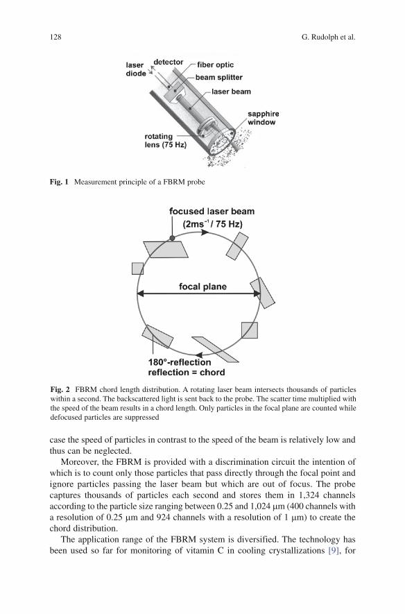
128 G. Rudolph et al.
case the speed of particles in contrast to the speed of the beam is relatively low and thus can be neglected.
Moreover, the FBRM is provided with a discrimination circuit the intention of which is to count only those particles that pass directly through the focal point and ignore particles passing the laser beam but which are out of focus. The probe captures thousands of particles each second and stores them in 1,324 channels according to the particle size ranging between 0.25 and 1,024 mm (400 channels with a resolution of 0.25 mm and 924 channels with a resolution of 1 mm) to create the chord distribution.
The application range of the FBRM system is diversified. The technology has been used so far for monitoring of vitamin C in cooling crystallizations [9], for
Fig. 1 Measurement principle of a FBRM probe
Fig. 2 FBRM chord length distribution. A rotating laser beam intersects thousands of particles within a second. The backscattered light is sent back to the probe. The scatter time multiplied with the speed of the beam results in a chord length. Only particles in the focal plane are counted while defocused particles are suppressed
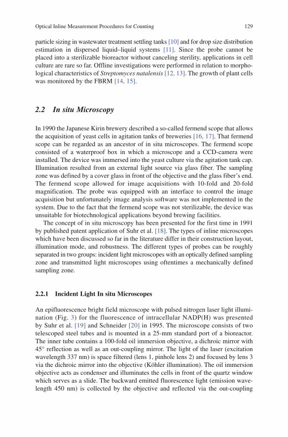
Optical Inline Measurement Procedures for Counting 129
particle sizing in wastewater treatment settling tanks [10] and for drop size distribution estimation in dispersed liquid–liquid systems [11]. Since the probe cannot be placed into a sterilizable bioreactor without canceling sterility, applications in cell culture are rare so far. Offline investigations were performed in relation to morpho-logical characteristics of Streptomyces natalensis [12, 13]. The growth of plant cells was monitored by the FBRM [14, 15].
2.2 In situ Microscopy
In 1990 the Japanese Kirin brewery described a so-called fermend scope that allows the acquisition of yeast cells in agitation tanks of breweries [16, 17]. That fermend scope can be regarded as an ancestor of in situ microscopes. The fermend scope consisted of a waterproof box in which a microscope and a CCD-camera were installed. The device was immersed into the yeast culture via the agitation tank cap. Illumination resulted from an external light source via glass fiber. The sampling zone was defined by a cover glass in front of the objective and the glass fiber’s end. The fermend scope allowed for image acquisitions with 10-fold and 20-fold magnification. The probe was equipped with an interface to control the image acquisition but unfortunately image analysis software was not implemented in the system. Due to the fact that the fermend scope was not sterilizable, the device was unsuitable for biotechnological applications beyond brewing facilities.
The concept of in situ microscopy has been presented for the first time in 1991 by published patent application of Suhr et al. [18]. The types of inline microscopes which have been discussed so far in the literature differ in their construction layout, illumination mode, and robustness. The different types of probes can be roughly separated in two groups: incident light microscopes with an optically defined sampling zone and transmitted light microscopes using oftentimes a mechanically defined sampling zone.
2.2.1 Incident Light In situ Microscopes
An epifluorescence bright field microscope with pulsed nitrogen laser light illumi-nation (Fig. 3) for the fluorescence of intracellular NADP(H) was presented by Suhr et al. [19] and Schneider [20] in 1995. The microscope consists of two telescoped steel tubes and is mounted in a 25-mm standard port of a bioreactor. The inner tube contains a 100-fold oil immersion objective, a dichroic mirror with 45° reflection as well as an out-coupling mirror. The light of the laser (excitation wavelength 337 nm) is space filtered (lens 1, pinhole lens 2) and focused by lens 3 via the dichroic mirror into the objective (Köhler illumination). The oil immersion objective acts as condenser and illuminates the cells in front of the quartz window which serves as a slide. The backward emitted fluorescence light (emission wave-length 450 nm) is collected by the objective and reflected via the out-coupling
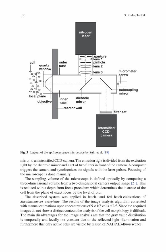
130 G. Rudolph et al.
mirror to an intensified CCD-camera. The emission light is divided from the excitation light by the dichroic mirror and a set of two filters in front of the camera. A computer triggers the camera and synchronizes the signals with the laser pulses. Focusing of the microscope is done manually.
The sampling volume of the microscope is defined optically by computing a three-dimensional volume from a two-dimensional camera output image [21]. This is realized with a depth from focus procedure which determines the distance of the cell from the plane of exact focus by the level of blur.
The described system was applied in batch- and fed batch-cultivations of Saccharomyces cerevisiae. The results of the image analysis algorithm correlated with manual estimations up to concentrations of 5 × 10⁸ cells mL−1. Since the acquired images do not show a distinct contour, the analysis of the cell morphology is difficult. The main disadvantages for the image analysis are that the gray value distribution is temporally and locally not constant due to the reflected light illumination and furthermore that only active cells are visible by reason of NADP(H)-fluorescence.
Fig. 3 Layout of the epifluorescence microscope by Suhr et al. [19]
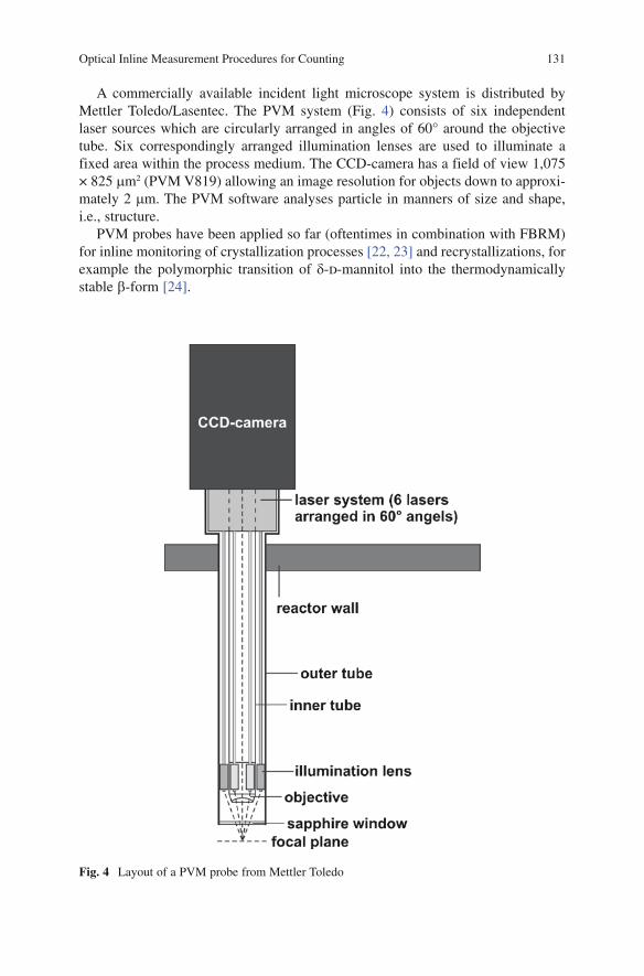
Optical Inline Measurement Procedures for Counting 131
A commercially available incident light microscope system is distributed by Mettler Toledo/Lasentec. The PVM system (Fig. 4) consists of six independent laser sources which are circularly arranged in angles of 60° around the objective tube. Six correspondingly arranged illumination lenses are used to illuminate a fixed area within the process medium. The CCD-camera has a field of view 1,075 × 825 mm2 (PVM V819) allowing an image resolution for objects down to approxi-mately 2 mm. The PVM software analyses particle in manners of size and shape, i.e., structure.
PVM probes have been applied so far (oftentimes in combination with FBRM) for inline monitoring of crystallization processes [22, 23] and recrystallizations, for example the polymorphic transition of d-d-mannitol into the thermodynamically stable b-form [24].
Fig. 4 Layout of a PVM probe from Mettler Toledo
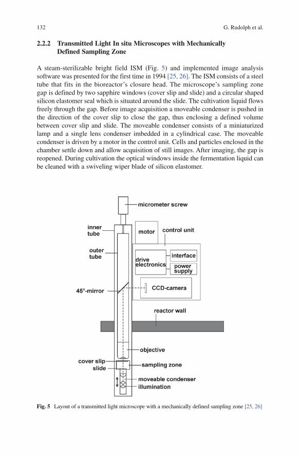
132 G. Rudolph et al.
2.2.2 Transmitted Light In situ Microscopes with Mechanically Defined Sampling Zone
A steam-sterilizable bright field ISM (Fig. 5) and implemented image analysis software was presented for the first time in 1994 [25, 26]. The ISM consists of a steel tube that fits in the bioreactor’s closure head. The microscope’s sampling zone gap is defined by two sapphire windows (cover slip and slide) and a circular shaped silicon elastomer seal which is situated around the slide. The cultivation liquid flows freely through the gap. Before image acquisition a moveable condenser is pushed in the direction of the cover slip to close the gap, thus enclosing a defined volume between cover slip and slide. The moveable condenser consists of a miniaturized lamp and a single lens condenser imbedded in a cylindrical case. The moveable condenser is driven by a motor in the control unit. Cells and particles enclosed in the chamber settle down and allow acquisition of still images. After imaging, the gap is reopened. During cultivation the optical windows inside the fermentation liquid can be cleaned with a swiveling wiper blade of silicon elastomer.
Fig. 5 Layout of a transmitted light microscope with a mechanically defined sampling zone [25, 26]

Optical Inline Measurement Procedures for Counting 133
An achromatic lens with 20-fold magnification is mounted in the inner tube. Focusing is only possible manually and takes place with a micrometer screw. A 45°-mirror reflects the incoming light onto a CCD-camera in the control unit. The image data are stored on a PC and are evaluated by an image analysis program in regard to parameters such as cell concentration and average cell diameter/cell volume.
With this system cultivations of S. cerevisiae were monitored and the generated images were evaluated with yeast cell analysis algorithms. In these experiments the cell concentration estimated by the ISM correlated almost linearly with hemocy-tometer counting up to concentrations of 108 cells mL−1. A general disadvantage of this system is the construction of the sampling zone which does not allow variations of the enclosed volume. Furthermore, the wiper blade must be declared unsuitable for industrial applications.
An autoclaveable ISM with an adjustable sampling zone and an integrated clean-ing mechanism (Fig. 6) is presented by Frerichs [27]. The microscope consists of two steel tubes. The inner tube contains a 20-fold magnifying objective and is focused manually via a micrometer screw. A 45°-mirror inside in the inner tube reflects the incoming light towards a CCD-camera which is positioned orthogonally to the optical path. The submerged end of the ISM contains the illuminator consisting of a miniaturized lamp, a condenser lens, and a stepper motor to adjust the opening of the sampling zone slid by moving the illuminator up or down. The sampling zone itself is represented by two sapphire windows (slide and cover slip) enclosing the adjusted volume. The cover slip window is fixed in front of the inner tube whereas the slide window sits on top of the moveable illuminator.
For cleaning purposes it is possible to retract the sampling zone from the reactor room into a flushing chamber that allows cleaning the sapphire windows from attaching
Fig. 6 ISM probe by Frerichs [27] with a retract mechanism for maintenance during cultivation

134 G. Rudolph et al.
cells or solid medium components without harming the process sterility. This retract-mechanism is similar to the Intrac system from Mettler Toledo. Therefore the sampling zone is steam sterilized before it is reinserted into the culture medium.
The system designed by Frerichs shows in principal the possibility of inline monitoring of long-term cultivations over several weeks with in situ microscopy due to the cleaning mechanism. However, the image quality of the microscope turned out to be insufficient for a fully automated image analysis. Furthermore, the position of the motor below the illuminator is problematical as maintenance of the motor is impossible during cultivation.
A constructional advance in this regard is the modular designed ISM system [28, 29] depicted in Fig. 7. Like the first type this microscope contains a height-adjustable flow sampling zone which can be adapted to changing process conditions. However, unlike other ISM systems, this type consists of three tubes – an outer probe tube, a sampling zone tube for adjusting the slid opening, and an inner objective tube. The miniaturized lamp in the illuminator is replaced with a LED emitting at a wavelength of 525 nm. In this wavelength range the CCD-camera reaches its maximum spectral sensitivity. The CCD-camera which is connected to the inner tube and the objective is mounted on linear stage with cross roller bearings. This linear stage and a second stage which is linked with the outer tube are mounted on a profile with U-shape. The exact adjustment of the sampling zone volume flow as well as focusing is operated by a set of two stepper motors plus micrometer heads. For autoclavation the complete U profile with its optical and electrical components is removed from the probe tube. The image quality of the ISM is comparable to conventional microscopes. Depending on the application, i.e., monitoring of yeast or mammalian cells, different objectives (4-fold, 10-fold or 20-fold magnification) can be mounted on the objective tube.
Fig. 7 Layout of an ISM described by Frerichs and Joeris [28, 29]
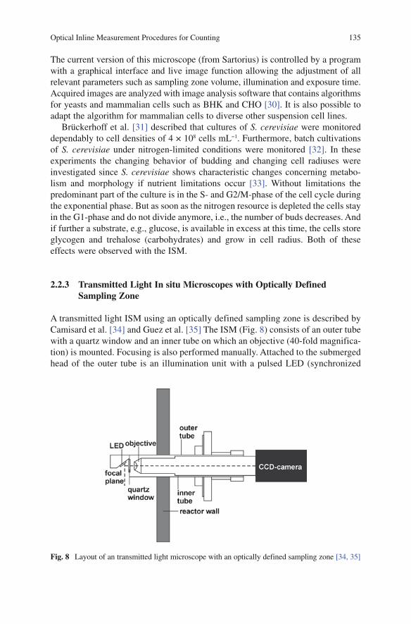
Optical Inline Measurement Procedures for Counting 135
The current version of this microscope (from Sartorius) is controlled by a program with a graphical interface and live image function allowing the adjustment of all relevant parameters such as sampling zone volume, illumination and exposure time. Acquired images are analyzed with image analysis software that contains algorithms for yeasts and mammalian cells such as BHK and CHO [30]. It is also possible to adapt the algorithm for mammalian cells to diverse other suspension cell lines.
Brückerhoff et al. [31] described that cultures of S. cerevisiae were monitored dependably to cell densities of 4 × 10⁸ cells mL−1. Furthermore, batch cultivations of S. cerevisiae under nitrogen-limited conditions were monitored [32]. In these experiments the changing behavior of budding and changing cell radiuses were investigated since S. cerevisiae shows characteristic changes concerning metabo-lism and morphology if nutrient limitations occur [33]. Without limitations the predominant part of the culture is in the S- and G2/M-phase of the cell cycle during the exponential phase. But as soon as the nitrogen resource is depleted the cells stay in the G1-phase and do not divide anymore, i.e., the number of buds decreases. And if further a substrate, e.g., glucose, is available in excess at this time, the cells store glycogen and trehalose (carbohydrates) and grow in cell radius. Both of these effects were observed with the ISM.
2.2.3 Transmitted Light In situ Microscopes with Optically Defined Sampling Zone
A transmitted light ISM using an optically defined sampling zone is described by Camisard et al. [34] and Guez et al. [35] The ISM (Fig. 8) consists of an outer tube with a quartz window and an inner tube on which an objective (40-fold magnifica-tion) is mounted. Focusing is also performed manually. Attached to the submerged head of the outer tube is an illumination unit with a pulsed LED (synchronized
Fig. 8 Layout of an transmitted light microscope with an optically defined sampling zone [34, 35]

136 G. Rudolph et al.
with the trigger of the CCD-camera) as light source. The LED having a wave-length of 610 nm is placed angularly opposite the quartz window. Like the epifluo-rescence ISM (see Sect. 2.2.1) this microscope does not enclose a defined volume mechanically. Thus the volume for the calculation of the cell concentration is also defined optically with the depth from focus procedure [21]. Subsequent to acquisi-tion, an image analysis algorithm processes the image data in regard to cell con-centration and cell size distribution.
This ISM type was applied in yeast batch cultivations of Hansenula anomala. The comparison between microscope count and offline count corresponds to con-centrations of 7 × 10⁸ cells mL−1. During a cultivation of H. anomala the osmotic pressure was increased by the addition of glycerin to let the cells contract. This cell contraction (decrease of mean cell radius) could be measured with the analysis algorithm. Apart from yeasts, that microscope version has been used to monitor cultivations of BALB/c hybridoma cells.
3 New Applications and Developments
3.1 Visualization of Morphological Changes
Apart from monitoring cell density and cell size distribution the full potential is not fully tapped by any means. Inline microscopes offer the possibility to visualize morphological changes of cells, thus giving direct information about a culture’s status. The flagellate Euglena gracilis exemplifies a type of microorganisms which show great morphological distinctions depending from environmental conditions. Under heterotrophic conditions these flagellates store large amounts of the carbohydrate paramylon which belongs to b-1,3-glucans. Such glucans were examined intensively in the last few years by the pharmaceutical and food industries due to its immune-stimulating and cell-regenerating properties [36, 37]. Therefore possible applications of paramylon are in the fields of functional food, pharmaceutical production and cosmetics. Under optimal cultivation conditions the cells show a cylindrical form. They are filled completely with paramylon while being extremely mobile.
By unsuitable environmental conditions such as insufficiencies of nutrients, oxygen, light, or unsuitable temperatures, a morphology change is induced. The mobility of E. gracilis decreases and the cells start to become ball-shaped. Figure 9 depicts the culture state of E. gracilis at three different times. Figure 9a shows the cells in the exponen-tial growing phase when they have stored large amounts of paramylon and their cylindrical shape indicates optimal culture conditions. In contrast, Fig. 9b shows the cell in the steady state at beginning of nutrient insufficiencies. The cells have a more slender shape than in the exponential phase and, sporadically, excavations can be spotted in the cells. This morphological change indicates the decomposition of paramylon which has metabolized due to the insufficiencies of nutrients. Beside morphological

Optical Inline Measurement Procedures for Counting 137
change decreasing mobility can also be observed. Finally, Fig. 9c depicts the culture at continuing unsuitable environmental conditions. The amount of ball-shaped cells at this time is nearly 90%. Much cell debris and paramylon kernels in the image indi-cate that most of the cells are already apoptotic and lysed.
3.2 Monitoring of Adherent Cells in Microcarrier Culture
The use of microcarriers is an established standard method when cultivating adherent cells. Most types of microcarriers are unsuitable for inline-microscopic observations due to their opacity, i.e., light reflections. Cytodex 1 microcarriers are an exception because of their transparency. Figure 10 depicts the course of such microcarrier cultivation with adherent NIH-3T3 cells (Mus musculus) from inoculation to harvest after 155 h. The consecutive steps of the microcarrier colonization – cell adhesion on the microcarrier surface, morphological change of cell shape, proliferation and complete overgrowth of the microcarrier – are clearly recognizable. The monitoring of microcarrier cultures enables the possibility to gain information about important parameters such as the plating efficiency and the mean level of colonization [38]. This information can be helpful to determinate the optimal time for cell harvest.
3.3 Cell Density Estimation in Three-Dimensional Cell Clusters
In 2005, Martinez et al. [30] proposed an algorithm for automatic cell density estimation inside of a bioreactor by analysis of an intensity image of the sampling zone captured by the CCD-camera of the ISM. First, the cells present in the captured intensity image are automatically counted. Then the cell density is computed as the quotient between the counted number of cells and the sampling zone volume. The novelty of this algorithm is that it is also able to count the cells which aggregate parallel to the sample zone forming two-dimensional single layer clusters.
Fig. 9 Inline cultivation images of E. gracilis (10-fold magnification) at different stages. a Exponential growing phase. b Steady state at the beginning of nutrient insufficiencies. c Phase with predominantly nonviable, i.e., lysed cells

138 G. Rudolph et al.
Assuming that the cells are round, that they are almost of the same size, and that they build two-dimensional single layer clusters only, the number of cells of each cluster is estimated as the quotient between the area of the image region of the clus-ter and the area of a circle with radius equal to the average cell radius of the cluster. The image regions of the clusters are determined (segmented) by maximum-likeli-hood global thresholding the local intensity variance at each pixel position of the image [39]. In [40], a local thresholding is also applied after global thresholding to improve the accuracy of the cell cluster image region segmentation. The average cell radius of the cells in each cluster is estimated by maximizing the variance of the circular Hough transform of the edges in the image region of the cluster. The edges are extracted by applying the smallest univalue segment assimilating nucleus (SUSAN) algorithm [41]. Finally, the number of cells present in the captured inten-sity image is computed as the sum of the number of cells estimated in all clusters. Experimental results with cultures of mammalian BHK cells showed that the cell density estimation algorithm works well only for cultures up to cell densities of 5 × 10⁶ cells mL−1. For higher cell concentrations the estimated cell density is less than
Fig. 10 Microcarrier based cultivation of adherent NIH-3T3 cells (fourfold magnification). After inoculation the cells settle down on the microcarrier surface, change their morphology and proliferate. After 155 h all microcarriers are completely overgrown
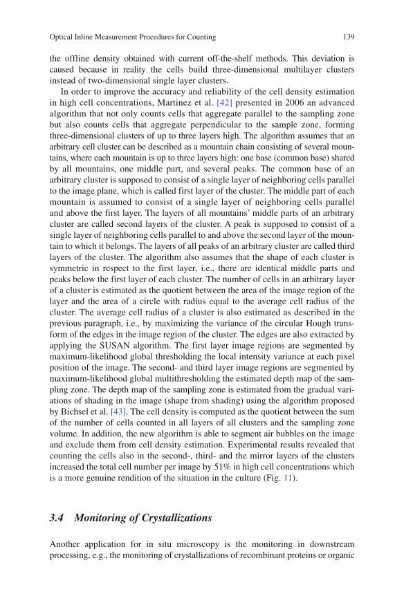
Optical Inline Measurement Procedures for Counting 139
the offline density obtained with current off-the-shelf methods. This deviation is caused because in reality the cells build three-dimensional multilayer clusters instead of two-dimensional single layer clusters.
In order to improve the accuracy and reliability of the cell density estimation in high cell concentrations, Martinez et al. [42] presented in 2006 an advanced algorithm that not only counts cells that aggregate parallel to the sampling zone but also counts cells that aggregate perpendicular to the sample zone, forming three-dimensional clusters of up to three layers high. The algorithm assumes that an arbitrary cell cluster can be described as a mountain chain consisting of several moun-tains, where each mountain is up to three layers high: one base (common base) shared by all mountains, one middle part, and several peaks. The common base of an arbitrary cluster is supposed to consist of a single layer of neighboring cells parallel to the image plane, which is called first layer of the cluster. The middle part of each mountain is assumed to consist of a single layer of neighboring cells parallel and above the first layer. The layers of all mountains’ middle parts of an arbitrary cluster are called second layers of the cluster. A peak is supposed to consist of a single layer of neighboring cells parallel to and above the second layer of the moun-tain to which it belongs. The layers of all peaks of an arbitrary cluster are called third layers of the cluster. The algorithm also assumes that the shape of each cluster is symmetric in respect to the first layer, i.e., there are identical middle parts and peaks below the first layer of each cluster. The number of cells in an arbitrary layer of a cluster is estimated as the quotient between the area of the image region of the layer and the area of a circle with radius equal to the average cell radius of the cluster. The average cell radius of a cluster is also estimated as described in the previous paragraph, i.e., by maximizing the variance of the circular Hough trans-form of the edges in the image region of the cluster. The edges are also extracted by applying the SUSAN algorithm. The first layer image regions are segmented by maximum-likelihood global thresholding the local intensity variance at each pixel position of the image. The second- and third layer image regions are segmented by maximum-likelihood global multithresholding the estimated depth map of the sam-pling zone. The depth map of the sampling zone is estimated from the gradual vari-ations of shading in the image (shape from shading) using the algorithm proposed by Bichsel et al. [43]. The cell density is computed as the quotient between the sum of the number of cells counted in all layers of all clusters and the sampling zone volume. In addition, the new algorithm is able to segment air bubbles on the image and exclude them from cell density estimation. Experimental results revealed that counting the cells also in the second-, third- and the mirror layers of the clusters increased the total cell number per image by 51% in high cell concentrations which is a more genuine rendition of the situation in the culture (Fig. 11).
3.4 Monitoring of Crystallizations
Another application for in situ microscopy is the monitoring in downstream processing, e.g., the monitoring of crystallizations of recombinant proteins or organic
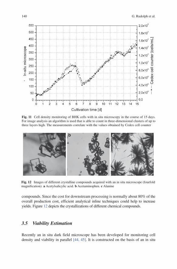
140 G. Rudolph et al.
compounds. Since the cost for downstream processing is normally about 80% of the overall production cost, efficient analytical inline techniques could help to increase yields. Figure 12 depicts the crystallizations of different chemical compounds.
3.5 Viability Estimation
Recently an in situ dark field microscope has been developed for monitoring cell density and viability in parallel [44, 45]. It is constructed on the basis of an in situ
Fig. 11 Cell density monitoring of BHK cells with in situ microscopy in the course of 15 days. For image analysis an algorithm is used that is able to count in three-dimensional clusters of up to three layers high. The measurements correlate with the values obtained by Cedex cell counter
Fig. 12 Images of different crystalline compounds acquired with an in situ microscope (fourfold magnification). a Acetylsalicylic acid. b Acetaminophen. c Alanine
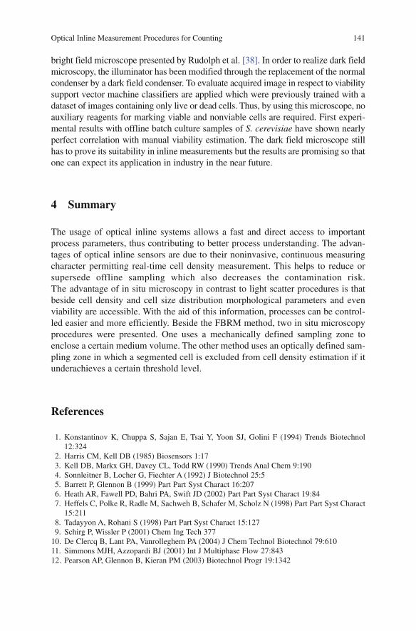
Optical Inline Measurement Procedures for Counting 141
bright field microscope presented by Rudolph et al. [38]. In order to realize dark field microscopy, the illuminator has been modified through the replacement of the normal condenser by a dark field condenser. To evaluate acquired image in respect to viability support vector machine classifiers are applied which were previously trained with a dataset of images containing only live or dead cells. Thus, by using this microscope, no auxiliary reagents for marking viable and nonviable cells are required. First experi-mental results with offline batch culture samples of S. cerevisiae have shown nearly perfect correlation with manual viability estimation. The dark field microscope still has to prove its suitability in inline measurements but the results are promising so that one can expect its application in industry in the near future.
4 Summary
The usage of optical inline systems allows a fast and direct access to important process parameters, thus contributing to better process understanding. The advan-tages of optical inline sensors are due to their noninvasive, continuous measuring character permitting real-time cell density measurement. This helps to reduce or supersede offline sampling which also decreases the contamination risk. The advantage of in situ microscopy in contrast to light scatter procedures is that beside cell density and cell size distribution morphological parameters and even viability are accessible. With the aid of this information, processes can be control-led easier and more efficiently. Beside the FBRM method, two in situ microscopy procedures were presented. One uses a mechanically defined sampling zone to enclose a certain medium volume. The other method uses an optically defined sam-pling zone in which a segmented cell is excluded from cell density estimation if it underachieves a certain threshold level.
References
1. Konstantinov K, Chuppa S, Sajan E, Tsai Y, Yoon SJ, Golini F (1994) Trends Biotechnol 12:324
2. Harris CM, Kell DB (1985) Biosensors 1:17 3. Kell DB, Markx GH, Davey CL, Todd RW (1990) Trends Anal Chem 9:190 4. Sonnleitner B, Locher G, Fiechter A (1992) J Biotechnol 25:5 5. Barrett P, Glennon B (1999) Part Part Syst Charact 16:207 6. Heath AR, Fawell PD, Bahri PA, Swift JD (2002) Part Part Syst Charact 19:84 7. Heffels C, Polke R, Radle M, Sachweh B, Schafer M, Scholz N (1998) Part Part Syst Charact
15:211 8. Tadayyon A, Rohani S (1998) Part Part Syst Charact 15:127 9. Schirg P, Wissler P (2001) Chem Ing Tech 377 10. De Clercq B, Lant PA, Vanrolleghem PA (2004) J Chem Technol Biotechnol 79:610 11. Simmons MJH, Azzopardi BJ (2001) Int J Multiphase Flow 27:843 12. Pearson AP, Glennon B, Kieran PM (2003) Biotechnol Progr 19:1342

142 G. Rudolph et al.
13. Pearson AP, Glennon B, Kieran PM (2004) J Chem Technol Biotechnol 79:1142 14. Jeffers P, Raposo S, Lima-Costa ME, Connolly P, Glennon B, Kieran PM (2003) Biotechnol
Lett 25:2023 15. Jeffers PT, Raposo S, Lima-Costa ME, Kieran P, Glennon B (2003) Abstr Paper Am Chem
Soc 225:U188 16. Konan (1990) Technical Report. Konan Camera Research Institute, Hyogo, Japan 17. Kumada J, Takahashi T, Nakatani K, Nagami K (1981) 18th European brewery convention
(EBC). Copenhagen, Denmark, p 293 18. Suhr H, Speil P, Wehnert G, Storhas W (1991) German Patent, DE 40,32,002 19. Suhr H-, Wehnert G, Schneider K, Bittner C, Scholz T, Geissler P, Jähne B, Scheper T (1995)
Biotechnol Bioeng 47:106 20. Schneider K (1995) PhD thesis, University of Hannover, Germany 21. Scholz T (1995) PhD thesis, University of Heidelberg, Germany 22. Barrett P, Glennon B (2002) Chem Eng Res Des 80:799 23. Kougoulos E, Jones AG, Jennings KH, Wood-Kaczmar MW (2005) J Cryst Growth 273:529 24. O’Sullivan B, Barrett P, Hsiao G, Carr A, Glennon B (2003) Org Process Res Dev 7:977 25. Bittner C (1994) PhD thesis, University of Hannover, Germany 26. Bittner C, Wehnert G, Scheper T (1998) Biotechnol Bioeng 60:24 27. Frerichs JG (2000) PhD thesis, University of Hannover, Germany 28. Frerichs JG, Joeris K, Konstantinov K, Scheper T (2002) Chem Ing Tech 74:1629 29. Joeris K, Frerichs JG, Konstantinov K, Scheper T (2002) Cytotechnology 38:129 30. Martinez G, Frerichs JG, Joeris K, Kontantinov K, Scheper T (2005) IEEE international con-
ference on acoustics, speech and signal processing (ICASSP), Philadelphia, PA, USA, p 497 31. Brückerhoff T, Frerichs JG, Joeris K, Konstantinov K, Scheper T (2005) In: Godia F, Fussenegger
M (eds) Animal cell technology meets genomics. Proceedings of the 18th ESACT meeting, Granada, Spain, May 11–14, 2003. Springer, Dordrecht, p 589
32. Brückerhoff T (2006) PhD thesis, University of Hannover, Germany 33. Larsson C, Vonstockar U, Marison I, Gustafsson L (1993) J Bacteriol 175:4809 34. Camisard V, Brienne JP, Baussart H, Hammann J, Suhr H (2002) Biotechnol Bioeng 78:73 35. Guez JS, Cassar JP, Wartelle F, Dhulster P, Suhr H (2004) J Biotechnol 111:335 36. Hetland G, Ohno N, Aaberge IS, Lovik M (2000) FEMS Immunol Med Microbiol 27:111 37. Ohno N, Miura NN, Nakajima M, Yadomae T (2000) Biol Pharm Bull 23:866 38. Rudolph G, Lindner P, Gierse A, Bluma A, Martinez G, Hitzmann B, Scheper T, Online
Monitoring of Microcarrier Based Fibroblast Cultivations with In situ Microscopy, Biotechnology and Bioengineering, Vol. 99, No. 1, January 1, 2008
39. Martinez G. “Criterion for Automatic Selection of the Most Suitable Maximum-Likelihood Thresholding Algorithm for extracting object from their background in a still image”, IAPR Conference on Machine Vision Applications, Tsukuba, Japan, 16–18 May 2005.
40. Espinoza E, Martinez G, Frerichs J-G, Scheper T (2006) 3rd IEEE international symposium on biomedical imaging, Arlington, Virginia, USA, p 542
41. Smith S, Bradly J (1997) Int J Comput Vis 23:45 42. Martinez G, Frerichs JG, Joeris K, Konstantinov K, Scheper T (2006) IEEE international
conference of acoustics, speech and signal processing (ICASSAP), Tolouse, France, p 581 43. Bichsel M and Pentland A. P “A Simple Algorithm for Shape from Shading”, CVPR
Conference on Computer Vision and Pattern Recognition, Champaign, Illinois, June 15–18, pp. 459– 463, 1992
44. Wei N, You J, Friehs K, Flaschel E, Nattkemper TW (2007) Biotechnol Lett 29:373 45. Wei N, You J, Friehs K, Flaschel E, Nattkemper TW (2007) Biotechnol Bioeng 97:1489

On the Design of Low-Cost Fluorescent Protein Biosensors
Leah Tolosa
1 Introduction
Proteins are the cell’s workhorses as they are involved in essentially all cellular activities. From the birth of a daughter cell until its death during apoptosis, proteins perform various functions as needed. Such versatility can be attributed to the seem-ingly infinite ways that the amino acids are sequenced in a polypeptide. The polypeptide backbone and each amino acid functional group contribute unique intermolecular interactions that determine the protein’s shape and size. However, more importantly, these interactions determine protein function, that is, its ability to interact with the external environment.
For the same reasons, proteins make ideal biorecognition elements for sensors (see below and Fig. 1). Protein enzymes and receptors developed unmatched sensitivity and selectivity for their substrates through millions of years of natural selection. In contrast, chemically synthesized artificial receptors seldom approach the same level of sophistication in ligand selectivity, sensitivity range and ease of production.
L. Tolosa Center for Advanced Sensor Technology, University of Maryland Baltimore County,Baltimore, MD21050, USA e-mail: [email protected]
Contents
1 Introduction ....................................................................................................................... 1432 Anatomy of a Fluorescent Protein Biosensor .................................................................... 1453 The Periplasmic Binding Proteins as Fluorescent Biosensors .......................................... 1464 From a Fluorescence Assay to a Fluorescent Biosensor ................................................... 1515 Summary ........................................................................................................................... 155References ............................................................................................................................... 156
Adv Biochem Engin/Biotechnol (2009) 116: 143–157DOI: 10.1007/10_2008_39© Springer-Verlag Berlin Heidelberg 200Published online: 04 April 2009
9
144 L. Tolosa
In addition, there is available to the sensor researcher an ever expanding library of proteins for various ligands important in all manner of application such as disease biomarkers, toxins, contaminants, drugs, etc. Using tools of genetic engineering, researchers can even go beyond known existing wild type proteins by introducing useful functional groups thereby tuning or even altering protein sensitivity and selec-tivity. This can be done by mutagenesis and directed evolution or by incorporation of unnatural amino acids during translation. Additionally, genes for the protein of interest can be inserted in vectors predesigned with handles for affinity purification or immo-bilization on a surface. Recombinant proteins can then be produced in large amounts in appropriate cellular hosts with very high reproducibility. In addition, chemical reactions involving the amino acids have become standard protocols. Thus, there are thousands of dyes, magnetic beads, nanoparticles or quantum dots designed to form covalent bonds with amino groups, sulfhydryl groups, carboxylic groups and other reactive functionalities in amino acids. It is not uncommon to conduct combinations of techniques, for example, the introduction of fluorescent labels or probes to proteins require in many cases, site-directed mutagenesis followed by covalent bonding of the fluorescent dye. Accordingly, two or more proteins can be combined to create hybrid or fusion proteins with multiple or altered functions. Indeed, research involving the green fluorescent protein and fluorescent proteins of a variety of colors has expanded by leaps and bounds in the last decade. Because these fluorescent proteins can be genetically encoded in cells, it is possible to observe various cellular processes in vivo. However, this topic has been reviewed extensively in the literature and, thus, will not be expounded on in this chapter.
Of the naturally occurring amino acids, tyrosine and tryptophan are inherently fluorescent with phenylalanine providing a negligible contribution. Thus, it has been possible to follow protein folding or denaturation, protein–ligand binding and protein–protein interactions by observing the changes in fluorescence of these two amino acids. However, the practicality of using tryptophan and tyrosine fluorescence for biosensing is limited by their UV excitation and emission that overlap significantly with the excitation and emission spectra of other biomolecules. The major obstacle to their use is separating the signal of interest from the background, particularly in complex mixtures and samples. To overcome this limitation, it has become widespread practice to label proteins with fluorescent probes. When attached to specific sites, the fluorescence from these probes provides an indirect signal of protein–ligand interactions that can be differentiated from background and is the basis for biosensing. A comprehensive list of fluorescent dyes classified according to the common chemical reactions for labeling proteins can be found in [1]. It should be mentioned that this handbook is also a product catalog.
The field of fluorescent protein biosensor research encompasses a broad range of areas including the genetically encoded proteins described above and antibody–antigen systems such as in fluorogenic Enzyme-Linked Immuno-Sorbent Assays (ELISA). It is difficult to cover the whole range of fluorescent protein biosensors; thus, we will limit the discourse here to the experience of our laboratory and others on a class of bacterial receptors called the periplasmic binding proteins (PBPs). The emphasis will be on the process of converting these receptors into a workable

On the Design of Low-Cost Fluorescent Protein Biosensors 145
biosensor device. Additionally, the progression of constructing a practical, i.e., low-cost and user-friendly, fluorescent sensor starting from the choice of protein receptor to engineering the signal transduction mechanism and the modular device to go with the whole system will be outlined.
2 Anatomy of a Fluorescent Protein Biosensor
The process of designing a biosensor always starts with the analyte of interest, say a disease biomarker, an active constituent or an impurity (Fig. 1). This is predicated by a perceived need, for example, a diagnostic device for cancer or the detection of virulent bacteria in food. Second, a recognition element, i.e., the protein, is identi-fied that will selectively interact with the analyte at the right sensitivity range and have the necessary properties amenable for the expected application. Sensor purists have argued that the protein receptor has to be immobilized on a substrate for it to be called a biosensor as shown in Fig. 1. Nevertheless, recent usage has been more flexible as in the use of fluorescent biosensors to describe fluorescent proteins in vivo [2–4]. The fluorescent probe attached to the protein is the signal transducer element which reports the interaction of the protein with analyte. For most applica-tions, the fluorophore should be able to report not only the presence of the analyte in the sample but also the concentration. Thus, the quantum yield, the excitation and emission wavelengths, fluorescence decay rate and other fluorescence proper-ties should allow for differentiation from the background (i.e., provide a significant signal-to-noise ratio). Appropriate optics and electronics then process the fluores-cence signal onto a readout system for visualization of the results. It should be noted that the opto-electronics design, at least initially, is contingent on the fluores-cence properties of the sensor. Nonetheless, this can be an iterative process where the cost-effectiveness and ease of assembly of the hardware can be improved further by adjusting accordingly the fluorescence properties of the biosensor.
Fig. 1 Schematic diagram of a fluorescent protein biosensor
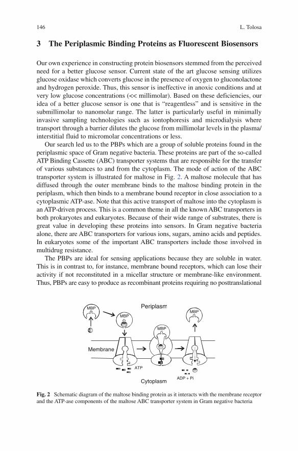
146 L. Tolosa
3 The Periplasmic Binding Proteins as Fluorescent Biosensors
Our own experience in constructing protein biosensors stemmed from the perceived need for a better glucose sensor. Current state of the art glucose sensing utilizes glucose oxidase which converts glucose in the presence of oxygen to gluconolactone and hydrogen peroxide. Thus, this sensor is ineffective in anoxic conditions and at very low glucose concentrations (<< millimolar). Based on these deficiencies, our idea of a better glucose sensor is one that is “reagentless” and is sensitive in the submillimolar to nanomolar range. The latter is particularly useful in minimally invasive sampling technologies such as iontophoresis and microdialysis where transport through a barrier dilutes the glucose from millimolar levels in the plasma/interstitial fluid to micromolar concentrations or less.
Our search led us to the PBPs which are a group of soluble proteins found in the periplasmic space of Gram negative bacteria. These proteins are part of the so-called ATP Binding Cassette (ABC) transporter systems that are responsible for the transfer of various substances to and from the cytoplasm. The mode of action of the ABC transporter system is illustrated for maltose in Fig. 2. A maltose molecule that has diffused through the outer membrane binds to the maltose binding protein in the periplasm, which then binds to a membrane bound receptor in close association to a cytoplasmic ATP-ase. Note that this active transport of maltose into the cytoplasm is an ATP-driven process. This is a common theme in all the known ABC transporters in both prokaryotes and eukaryotes. Because of their wide range of substrates, there is great value in developing these proteins into sensors. In Gram negative bacteria alone, there are ABC transporters for various ions, sugars, amino acids and peptides. In eukaryotes some of the important ABC transporters include those involved in multidrug resistance.
The PBPs are ideal for sensing applications because they are soluble in water. This is in contrast to, for instance, membrane bound receptors, which can lose their activity if not reconstituted in a micellar structure or membrane-like environment. Thus, PBPs are easy to produce as recombinant proteins requiring no posttranslational
Fig. 2 Schematic diagram of the maltose binding protein as it interacts with the membrane receptor and the ATP-ase components of the maltose ABC transporter system in Gram negative bacteria
Periplasm
Membrane
Cytoplasm
ATP
ADP + Pi
Mal
Mal
Mal
Mal
MBP
MBP
MBP
MBP
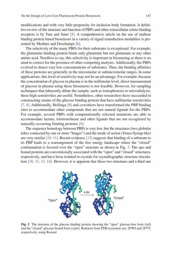
On the Design of Low-Cost Fluorescent Protein Biosensors 147
modifications and with very little propensity for inclusion body formation. A defini-tive review of the structure and function of PBPs and other extracellular solute-binding receptors is by Tam and Saier [5]. A comprehensive article on the use of maltose binding protein based biosensors in a variety of signal transduction modalities is pre-sented by Medintz and Deschamps [6].
The selectivity of the many PBPs for their substrates is exceptional. For example, the glutamine binding protein binds only glutamine but not glutamate or any other amino acid. Needless to say, this selectivity is important in biosensing as there is no need to correct for the presence of other competing analytes. Additionally, the PBPs evolved to detect very low concentrations of substrates. Thus, the binding affinities of these proteins are generally in the micromolar or submicromolar ranges. In some applications, this level of sensitivity may not be an advantage. For example, because the concentration of glucose in plasma is in the millimolar level, direct measurement of glucose in plasma using these biosensors is not feasible. However, for sampling techniques that inherently dilute the sample, such as iontophoresis or microdialysis, these high sensitivities are useful. Nonetheless, other researchers have succeeded in constructing strains of the glucose binding protein that have millimolar sensitivities [7, 8]. Additionally, Hellinga [9] and coworkers have transformed the PBP binding sites to accommodate other compounds that are not natural ligands for the PBPs. For example, several PBPs with computationally selected mutations are able to accommodate lactate, trinitrotoluene and other ligands that are not recognized by naturally-occurring binding proteins [9].
The sequence homology between PBPs is very low, but the structures (two globular lobes connected by one or more “hinges”) and the mode of action (Venus flytrap-like) are very similar [10, 11]. Recent evidence [12] suggests that binding of a substrate to its PBP leads to a rearrangement of the free energy landscape where the “closed” conformation is favored over the “open” structure as shown in Fig. 3. The apo and bound proteins are conventionally associated with the “open” and “closed” structures, respectively, and have been isolated in crystals for crystallographic structure elucida-tion [10, 11, 13, 14]. However, it is apparent that these two structures and a third one
Fig. 3 The structure of the glucose binding protein showing the “open” glucose-free form (left) and the “closed” glucose-bound form (right). Redrawn from PDB accession nos. 2FW0 and 2FVY, respectively, using Rasmol
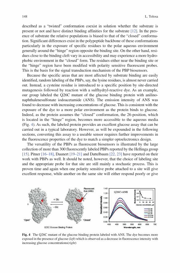
148 L. Tolosa
described as a “twisted” conformation coexist in solution whether the substrate is present or not and have distinct binding affinities for the substrate [12]. In the pres-ence of substrate the relative populations is biased to that of the “closed” conforma-tion. Significant differences exist in the polypeptide backbone of these conformations particularly in the exposure of specific residues to the polar aqueous environment generally around the “hinge” region opposite the binding site. On the other hand, resi-dues close to the binding cleft vary in accessibility and may experience a more hydro-phobic environment in the “closed” form. The residues either near the binding site or the “hinge” region have been modified with polarity sensitive fluorescent probes. This is the basis for the signal transduction mechanism of the PBP biosensors.
Because the specific areas that are most affected by substrate binding are easily identified, random labeling of the PBPs, say, the lysine residues, is almost never carried out. Instead, a cysteine residue is introduced to a specific position by site-directed mutagenesis followed by reaction with a sulfhydryl-reactive dye. As an example, our group labeled the Q26C mutant of the glucose binding protein with anilino-naphthalenesulfonate iodoacetamide (ANS). The emission intensity of ANS was found to decrease with increasing concentrations of glucose. This is consistent with the exposure of the dye to a more polar environment as the protein binds to glucose. Indeed, as the protein assumes the “closed” conformation, the 26-position, which is located in the “hinge” region, becomes more accessible to the aqueous media (Fig. 4). As such, the labeled protein provides an excellent glucose assay that can be carried out in a typical laboratory. However, as will be expounded in the following sections, converting this assay to a useable sensor requires further improvements in the fluorescence properties of the dye to match a simpler optoelectronics design.
The versatility of the PBPs as fluorescent biosensors is illustrated by the large collection of more than 300 fluorescently labeled PBPs reported by the Hellinga group [15]. Pitner [16–18], Daunert [19–21] and Dattelbaum [22, 23] have reported on their work with PBPs as well. It should be noted, however, that the choice of labeling site and the appropriate probe for that site are still mainly a stochastic process. This is proven time and again when one polarity sensitive probe attached to a site will give excellent response, while another on the same site will either respond poorly or give
Fig. 4 The Q26C mutant of the glucose binding protein labeled with ANS. The dye becomes more exposed in the presence of glucose (left) which is observed as a decrease in fluorescence intensity with increasing glucose concentrations(right)

On the Design of Low-Cost Fluorescent Protein Biosensors 149
no response at all. Even closely related fluorescent probes may present a wide range of usability in assays or as sensors. Figure 5 shows the varying fluorescence responses of three naphthalene derivatives attached to the 26-position in the glucose binding protein. It is obvious here that the ANS-labeled glucose binding protein provides the best response. Attempts to predict optimal sites for labeling even with a single dye have brought about minimal success. Starting off on the reported structures, molecular calculations of changes in the alpha-carbon distances and relative solvent accessibilities of amino acid residues provide only partial information on the eventual fluorescence response of the labeled protein. This indicates the complexity of interactions between dye, protein and environment. As a good example, in the study by Dattelbaum et al. [23] of the maltose binding protein labeled with the dye, N-((2-(iodoacetoxy)-ethyl)-N-methyl)-amino-7-nitrobenz-2-oxa-1,3-diazole (NBD), calculations suggested posi-tions 92, 95 and 233 to be appropriate sites for labeling. Nonetheless, the labeled proteins provided a mélange of results that do not necessarily conform to expectations. In Fig. 6, D95C-NBD presents the largest variation in fluorescence (left) but shows the least change in accessibility to quenching by iodide (right). Thus, solvent accessibility is not sufficient to predict the behavior of the fluorophore-labeled protein. Further molecular calculations and mutational studies pointed to the interaction of NBD with two tyrosine residues (171 and 176) in the vicinity of the 95 position. Even so, this was not apparent a priori and could not have been used to predict the observed responses.
Fig. 5 Closely related naphthalene dyes covalently attached to the Q26C position of GBP exhibit varying response in the presence of the same concentration of glucose
Q26C Glucose Binding Protein Labeled with Naphthalene
Derivatives
Maximum Change in
Fluorescence
CH2 C NH
O
NH
SO3−Na+
S
ANS
Protein 45%
SO3−Na+
NHCH2CH2HNC
O
CH2S
EDANS
Protein15%
C
O
CH2S
Acrylodan
Protein
N(CH3)2
~2%
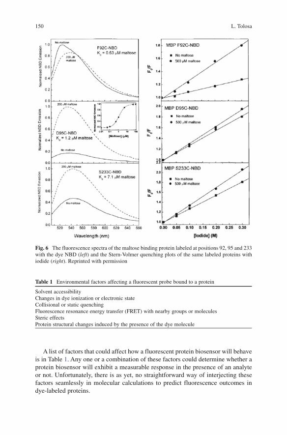
150 L. Tolosa
A list of factors that could affect how a fluorescent protein biosensor will behave is in Table 1. Any one or a combination of these factors could determine whether a protein biosensor will exhibit a measurable response in the presence of an analyte or not. Unfortunately, there is as yet, no straightforward way of interjecting these factors seamlessly in molecular calculations to predict fluorescence outcomes in dye-labeled proteins.
Table 1 Environmental factors affecting a fluorescent probe bound to a protein
Solvent accessibilityChanges in dye ionization or electronic stateCollisional or static quenchingFluorescence resonance energy transfer (FRET) with nearby groups or moleculesSteric effectsProtein structural changes induced by the presence of the dye molecule
Fig. 6 The fluorescence spectra of the maltose binding protein labeled at positions 92, 95 and 233 with the dye NBD (left) and the Stern-Volmer quenching plots of the same labeled proteins with iodide (right). Reprinted with permission
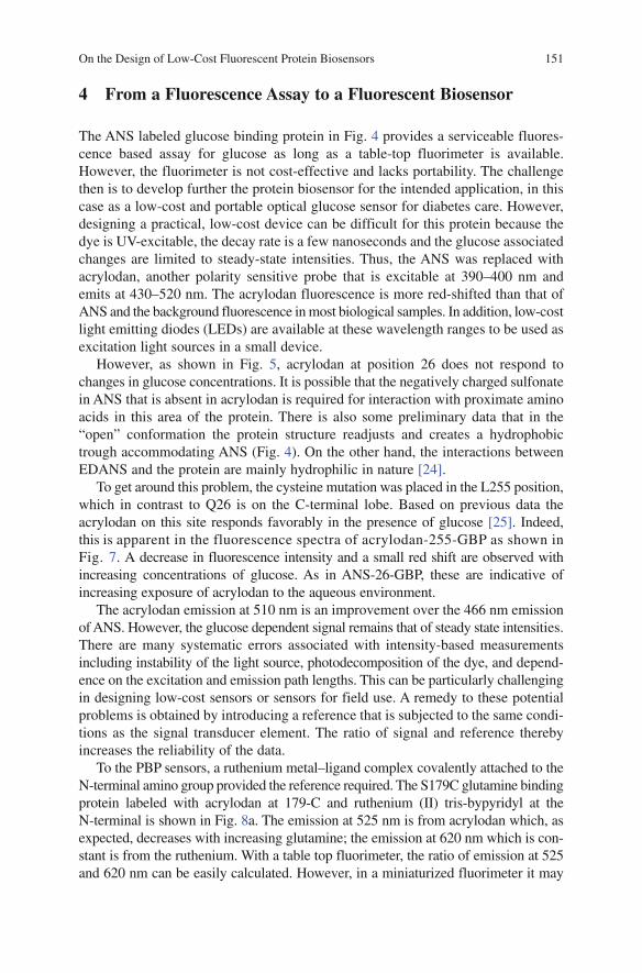
On the Design of Low-Cost Fluorescent Protein Biosensors 151
4 From a Fluorescence Assay to a Fluorescent Biosensor
The ANS labeled glucose binding protein in Fig. 4 provides a serviceable fluores-cence based assay for glucose as long as a table-top fluorimeter is available. However, the fluorimeter is not cost-effective and lacks portability. The challenge then is to develop further the protein biosensor for the intended application, in this case as a low-cost and portable optical glucose sensor for diabetes care. However, designing a practical, low-cost device can be difficult for this protein because the dye is UV-excitable, the decay rate is a few nanoseconds and the glucose associated changes are limited to steady-state intensities. Thus, the ANS was replaced with acrylodan, another polarity sensitive probe that is excitable at 390–400 nm and emits at 430–520 nm. The acrylodan fluorescence is more red-shifted than that of ANS and the background fluorescence in most biological samples. In addition, low-cost light emitting diodes (LEDs) are available at these wavelength ranges to be used as excitation light sources in a small device.
However, as shown in Fig. 5, acrylodan at position 26 does not respond to changes in glucose concentrations. It is possible that the negatively charged sulfonate in ANS that is absent in acrylodan is required for interaction with proximate amino acids in this area of the protein. There is also some preliminary data that in the “open” conformation the protein structure readjusts and creates a hydrophobic trough accommodating ANS (Fig. 4). On the other hand, the interactions between EDANS and the protein are mainly hydrophilic in nature [24].
To get around this problem, the cysteine mutation was placed in the L255 position, which in contrast to Q26 is on the C-terminal lobe. Based on previous data the acrylodan on this site responds favorably in the presence of glucose [25]. Indeed, this is apparent in the fluorescence spectra of acrylodan-255-GBP as shown in Fig. 7. A decrease in fluorescence intensity and a small red shift are observed with increasing concentrations of glucose. As in ANS-26-GBP, these are indicative of increasing exposure of acrylodan to the aqueous environment.
The acrylodan emission at 510 nm is an improvement over the 466 nm emission of ANS. However, the glucose dependent signal remains that of steady state intensities. There are many systematic errors associated with intensity-based measurements including instability of the light source, photodecomposition of the dye, and depend-ence on the excitation and emission path lengths. This can be particularly challenging in designing low-cost sensors or sensors for field use. A remedy to these potential problems is obtained by introducing a reference that is subjected to the same condi-tions as the signal transducer element. The ratio of signal and reference thereby increases the reliability of the data.
To the PBP sensors, a ruthenium metal–ligand complex covalently attached to the N-terminal amino group provided the reference required. The S179C glutamine binding protein labeled with acrylodan at 179-C and ruthenium (II) tris-bypyridyl at the N-terminal is shown in Fig. 8a. The emission at 525 nm is from acrylodan which, as expected, decreases with increasing glutamine; the emission at 620 nm which is con-stant is from the ruthenium. With a table top fluorimeter, the ratio of emission at 525 and 620 nm can be easily calculated. However, in a miniaturized fluorimeter it may
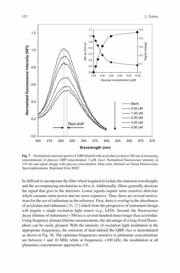
152 L. Tolosa
be difficult to incorporate the filter wheel required to isolate the emission wavelengths and the accompanying mechanism to drive it. Additionally, filters generally decrease the signal that goes to the detectors. Lower signals require more sensitive detectors which consume more power and are more expensive. Thus, there are several motiva-tions for the use of ruthenium as the reference. First, there is overlap in the absorbance of acrylodan and ruthenium [26, 27] which from the perspective of instrument design will require a single excitation light source (e.g., LED). Second, the fluorescence decay lifetime of ruthenium (~700 ns) is several hundred times longer than acrylodan. Using frequency domain lifetime measurements, the advantage of a long-lived fluoro-phore can be easily gleaned. With the intensity of excitation light modulated at the appropriate frequencies, the emission of dual-labeled Ru–QBP–Acr is demodulated as shown in Fig. 8b. The optimum frequencies sensitive to glutamine concentrations are between 1 and 10 MHz while at frequencies <100 kHz, the modulation at all glutamine concentrations approaches 1.0.
Fig. 7 Normalized emission spectra of GBP labeled with acrylodan excited at 380 nm in increasing concentrations of glucose. GBP concentration: 3 mM. Inset: Normalized fluorescence intensity at 510 nm and signal change with glucose concentration. Data were obtained on Varian Fluorescence Spectrophotometer. Reprinted from JDST
0.0
0.2
0.4
0.6
0.8
1.0
1.2
450 475 500 525 550 575 600 625 650 675 675
Wavelength (nm)
No
rmal
ized
flu
ore
scen
ce in
ten
sity
(N
FI)
Blank0.50 uM
1.00 uM2.00 uM
4.00 uM
9.90 uMRed shift
0.4
0.5
0.6
0.7
NF
I at 5
10 n
m
Sig
nal c
hang
e
0.8
0.9
1.0
1.1
0.00 2.00 4.00 6.00 8.00 10.00
Glucose concentration (µM)
0
0.1
0.2
0.3
0.4
0.5
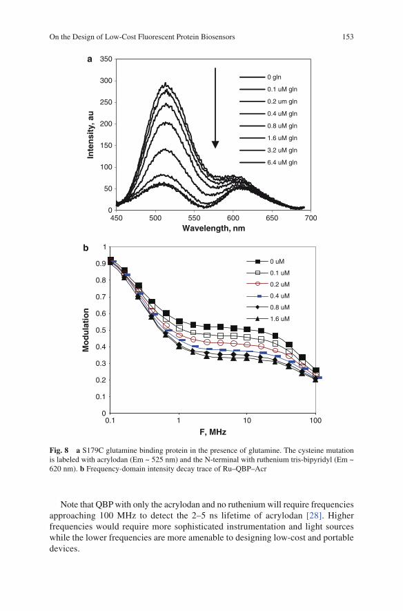
On the Design of Low-Cost Fluorescent Protein Biosensors 153
Note that QBP with only the acrylodan and no ruthenium will require frequencies approaching 100 MHz to detect the 2–5 ns lifetime of acrylodan [28]. Higher frequencies would require more sophisticated instrumentation and light sources while the lower frequencies are more amenable to designing low-cost and portable devices.
Fig. 8 a S179C glutamine binding protein in the presence of glutamine. The cysteine mutation is labeled with acrylodan (Em ~ 525 nm) and the N-terminal with ruthenium tris-bipyridyl (Em ~ 620 nm). b Frequency-domain intensity decay trace of Ru–QBP–Acr
0
50
100
150
200
250
300
350
450 500 550 600 650 700
Inte
nsi
ty, a
u
Wavelength, nm
0 gln
0.1 uM gln
0.2 um gln
0.4 uM gln
0.8 uM gln
1.6 uM gln
3.2 uM gln
6.4 uM gln
a
0
0.1
0.2
0.3
0.4
0.5
0.6
0.7
0.8
0.9
1
0.1 1 10 100
F, MHz
Mo
du
lati
on
0 uM
0.1 uM
0.2 uM
0.4 uM
0.8 uM
1.6 uM
b
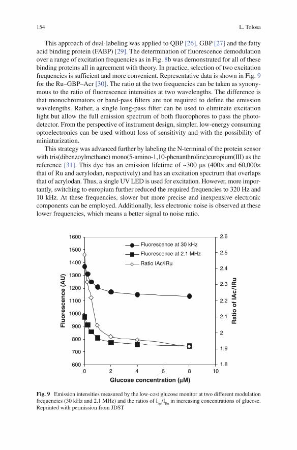
154 L. Tolosa
This approach of dual-labeling was applied to QBP [26], GBP [27] and the fatty acid binding protein (FABP) [29]. The determination of fluorescence demodulation over a range of excitation frequencies as in Fig. 8b was demonstrated for all of these binding proteins all in agreement with theory. In practice, selection of two excitation frequencies is sufficient and more convenient. Representative data is shown in Fig. 9 for the Ru–GBP–Acr [30]. The ratio at the two frequencies can be taken as synony-mous to the ratio of fluorescence intensities at two wavelengths. The difference is that monochromators or band-pass filters are not required to define the emission wavelengths. Rather, a single long-pass filter can be used to eliminate excitation light but allow the full emission spectrum of both fluorophores to pass the photo-detector. From the perspective of instrument design, simpler, low-energy consuming optoelectronics can be used without loss of sensitivity and with the possibility of miniaturization.
This strategy was advanced further by labeling the N-terminal of the protein sensor with tris(dibenzoylmethane) mono(5-amino-1,10-phenanthroline)europium(III) as the reference [31]. This dye has an emission lifetime of ~300 ms (400× and 60,000× that of Ru and acrylodan, respectively) and has an excitation spectrum that overlaps that of acrylodan. Thus, a single UV LED is used for excitation. However, more impor-tantly, switching to europium further reduced the required frequencies to 320 Hz and 10 kHz. At these frequencies, slower but more precise and inexpensive electronic components can be employed. Additionally, less electronic noise is observed at these lower frequencies, which means a better signal to noise ratio.
Fig. 9 Emission intensities measured by the low-cost glucose monitor at two different modulation frequencies (30 kHz and 2.1 MHz) and the ratios of I
Ac/I
Ru in increasing concentrations of glucose.
Reprinted with permission from JDST
600
700
800
900
1000
1100
1200
1300
1400
1500
1600
0 2 4 6 8 10
Glucose concentration (mM)
Flu
ore
scen
ce (
AU
)
1.8
1.9
2
2.1
2.2
2.3
2.4
2.5
2.6R
atio
of
IAc
/IR
u
Fluorescence at 30 kHz
Fluorescence at 2.1 MHz
Ratio IAc/IRu
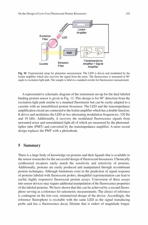
On the Design of Low-Cost Fluorescent Protein Biosensors 155
A representative schematic diagram of the instrument set-up for the dual labeled binding protein sensor is given in Fig. 10. This design is for 90° detection from the excitation light path similar to a standard fluorimeter but can be easily adapted to a cassette with an immobilized protein biosensor. The LED and the transimpedance amplification circuit are connected to the lockin amplifier which has a double function. It drives and modulates the LED at two alternating modulation frequencies, 320 Hz and 10 kHz. Additionally, it recovers the modulated fluorescence signals from unwanted noise and unmodulated light all of which are measured by the photomul-tiplier tube (PMT) and converted by the transimpedance amplifier. A more recent design replaces the PMT with a photodiode.
5 Summary
There is a large body of knowledge on proteins and their ligands that is available to the sensor researcher for the successful design of fluorescent biosensors. Chemically synthesized receptors rarely match the sensitivity and selectivity of proteins. Additionally, proteins are easily produced and manipulated through recombinant protein techniques. Although limitations exist in the prediction of signal response of proteins labeled with fluorescent probes, thoughtful experimentation can lead to useful, highly responsive fluorescent protein assays. Conversion of these assays into sensor devices may require additional manipulation of the fluorescence properties of the labeled proteins. We have shown that this can be achieved by a second fluoro-phore serving as a reference for ratiometric measurements. The choice of reference is contingent on the low-cost, miniaturized design of the device. Accordingly, the reference fluorophore is excitable with the same LED as the signal transducing probe and has a fluorescence decay lifetime that is orders of magnitude longer.
Fig. 10 Experimental setup for glutamine measurement. The LED is driven and modulated by the lockin amplifier which also recovers the signal from the noise. The fluorescence is measured at 90° angle to excitation light path. The sample is held in a standard cuvette for fluorescence measurement

156 L. Tolosa
Alternating illumination with intensity modulated light at two frequencies allows for ratiometric sensing without the need for bulky filter wheels while collecting the signals over a wide range of emission wavelengths. The result is a simple opto-electronics design that is cost-effective and small enough to be portable.
In summary, the process of designing protein-based fluorescent biosensors for practical applications requires the systematic collaboration of a cross-disciplinary group of molecular biologists, chemists and engineers.
References
1. Haugland R (2005) The handbook: a guide to fluorescent probes and labeling technologies, 10th edn. Molecular Probes – Invitrogen Corp, Eugene, OR
2. VanEngelenburg SB, Palmer AE (2008) Fluorescent biosensors of protein function. Curr Opin Chem Biol 12:60–65
3. Ai H-W, Hazelwood KL, Davidson MW, Campbell RE (2008) Fluorescent protein FRET pairs for ratiometric imaging of dual biosensors. Nat Methods 5(5):401–403
4. Guiliano KA, Taylor DL (1998) Fluorescent-protein biosensors: new tools for drug discovery. TIBTECH 16:135–140
5. Tam R, Saier MH (1993) Structural, functional and evolutionary relationships among extra-cellular solute-binding receptors of bacteria. Microbiol Rev 57(2):320–346
6. Medintz IL, Deschamps JR (2006) Maltose binding protein: a versatile platform for prototyping biosensing. Curr Opin Biotechnol 17:17–21
7. Sakaguchi-Mikami A, Taneoka A, Yamoto R, Ferri S, Sode K (2008) Engineering of ligand specificity of periplasmic binding protein for glucose. Biotech Lett. 30(8):1453–1460.
8. Amiss TJ, Sherman DB, Nycz CM, Andaluz SA, Pitner JB (2007) Engineering and rapid selection of a low-affinity glucose/galactose binding protein for a glucose biosensor. Protein Sci 16:2350–2359
9. Looger LL, Dwyer MA, Smith JJ, Hellinga HW (2003) Computational design of receptor and sensor proteins with novel functions. Nature 423:185
10. Hsiao CD, Sun YJ, Rose J, Wang BC (1996) The crystal structure of glutamine-binding protein from Escherichia coli. J Mol Biol 262:225–242
11. Sun YJ, Rose J, Wang BC, Hsiao CD (1998) The crystal structure of glutamine-binding protein complexed with glutamine at 1.94 Å resolution: comparisons with other amino acid binding protein. J Mol Biol 278:219–229
12. Messina TC, Talaga DS (2007) Protein free energy landscapes remodeled by ligand binding. Biophys J 93:579–585
13. Mowbray SL, Petsko GA (1983) The X-ray structure of the periplasmic galactose binding protein from Salmonella typhimurium at 3.0-Å resolution. J Biol Chem 258(13):7991–7997
14. Borrok MJ, Kiessling LL, Forest KT (2007) Conformational changes of glucose/galactose binding protein illuminated by open, unliganded and ultra-high-resolution ligand bound struc-tures. Protein Sci 16:1032–1041
15. Lorimer RM, Smith JJ, Dwyer MA, Looger LL, Sali KM, Paavola CD, Rizk SS, Sadigov SS, Conrad DW, Loew L, Hellinga HW (2002) Construction of a fluorescent biosensor family. Protein Sci 11:2655–2675
16. Thomas KJ, Sherman DB, Amiss TJ, Andaluz SA, Pitner JB (2006) A long-wavelength fluo-rescent glucose biosensor based on bioconjugates of galactose/glucose binding protein and Nile Red derivatives. Diab Technol Ther 8(3):261–268
17. Sherman DB, Pitner JB, Ambroise A, Thomas KJ (2006) Synthesis of thiol-reactive, long wavelength fluorescent phenoxazine derivatives for biosensor applications. Bioconjug Chem 17(2):387–392
On the Design of Low-Cost Fluorescent Protein Biosensors 157
18. Hsieh HV, Pfeiffer ZA, Amiss TJ, Sherman DB, Pitner JB (2004) Direct detection of glucose by surface plasmon resonance with bacterial glucose/galactose binding protein. Biosens Bioelectron 19(7):653–660
19. Hamorsky KT, Ensor CM, Wei Y, Daunert S (2008) A bioluminescent molecular switch for glucose. Angew Chem Int Ed 47:3718–3721
20. Salins LL, DeoSK, Daunert S (2004) Phosphate binding protein as the biorecognition element in a biosensor for phosphate. Sens Actuators B Chem 97(1):81–89
21. Ehrick JD, Deo SK, Browning TW, Bachas LG, Madou MJ, Daunert S (2005) Genetically engi-neered protein in hydrogels tailors stimuli-responsive characteristics. Nat Mater 4(4):298–302
22. Der BS, Dattelbaum JD (2007) Construction of a reagentless glucose biosensor using molecular exciton luminescence. Anal Biochem 375:132–140
23. Dattelbaum JD, Looger LL, Benson DE, Sali KM, Thompson RB, Hellinga HW (2005) Analysis of allosteric signal transduction mechanisms in an engineered fluorescent maltose biosensor. Protein Sci 14:284–289
24. Tolosa L, Harrison R, Rao G (2007) Design of optical protien-based biosensors. Proceedings of Asia Sense 2007 He third Asian conference on sensors, new domains in chemical, biological and physical sensing. pp 61–64
25. Marvin JS, Hellinga HW (1998) Engineering biosensors by introducing fluorescent allosteric signal transducers: construction of a novel glucose sensor. J Am Chem Soc 120:7–11
26. Ge X, Tolosa L, Rao G (2004) Dual-labeled glucose binding protein for ratiometric measurements of glucose. Anal Chem 76:1403–1410
27. Tolosa L, Ge X, Rao G (2003) Reagentless optical sensing of glutamine using a dual-emitting glutamine-binding protein. Anal Biochem 314:199–205
28. Dattelbaum JD, Lakowicz JR, (2001) Optical determination of glutamine using a genetically engineered protein. Anal Biochem 291(1):89–95
29. Bartolome A, Bardliving C, Rao G, Tolosa L (2005) Fatty acid sensor for low-cost lifetime-assisted ratiometric sensing using a fluorescent fatty acid binding protein. Anal Biochem 345:133–139
30. Ge X, Lam HT, Swati MJ, LaCourse WR, Rao G, Tolosa L, (2007) Comparing the perform-ance of the optical glucose assay based on the glucose binding protein with high performance anion-exchange chromatography with pulsed electrochemical detection: efforts to design a low-cost point-of-care glucose sensor. J Diab Sci Technol 1(6):864–872
31. Lam H, Kostov Y, Rao G, Tolosa L (2008) Low-cost optical lifetime assisted ratiometric glutamine sensor based on glutamine binding protein. Anal Biochem 383:61–67

Index
AAcetaminophen, ISM, 140Acetylsalicylic acid, ISM, 140Acid Orange 7, 117Acidity, cell culture media, 19Acrylodan-255-GBP, 151Alanine, ISM, 140Alcohol oxidase, 111Alcohols, 111Aluminum nanostructured substrates, 34Anilinonaphthalenesulfonate iodoacetamide
(ANS), 148Antibodies, 99, 112
anti-PCB, 116Arsenic, 118ATP Binding Cassette (ABC) transporter
systems, 146Atrazine, 116Avalanche photodiodes (APDs), 106
BBacillus stearothermophilus,
phenol-oxidizing, 112Benzene, 113Benzo(a)pyrene, 112Biomanufacturing, 74Biomolecules, association, metal nanoparticles, 38Biosensors, 99
chemical analytes, 111environmental applications, 101optical, 103photoluminescence-based, 100
Blu-ray disc players, 105
CCadmium, 119Carbon dioxide, 1, 24
Carbonic anhydrase, 119Carboxydiclorofluorescein
(CDCF), 20, 21Carboxyfluoresceins, 20Carboxynaphthofluorescein (CNF), 21Cell density estimation, three-dimensional cell
clusters, 137Cell size distribution, 125Chemical mixtures, 119Chemical terrorism, water
supplies, 101Chemometrics, multivariate data
analysis, 80Chlorocatechols, 117Chlorohexane, 116Chlorophenols, 117CO
2, 1, 24
Contaminated sites, characterization, 102Contamination, detection, 93Copper, 119Crystallization, 139Cyclodiene organochlorine, 116
DDichloroethane (DCA), 113Dioxins, 117DO (dissolved oxygen), 1, 12
EEndosulfan, 116Environmental monitoring,
102, 103Enzymes, 99, 104, 112Epifluorescence microscope, 129Escherichia coli fermentations, 79Ethanol, 1, 2, 11Euglena gracilis, 136
159

160 Index
FFatty acid binding protein (FABP), 154Fluorescence, 1, 29
assay, 151Fluorescence resonance energy transfer
(FRET), 30Fluorescent protein biosensors, anatomy, 145
periplasmic binding proteins, 146Fluorophore–metal interactions, 33Focused beam reflectance measurement
(FBRM), 125, 127
GGaN diodes, 105Gasoline, 119Gated detection method, 14Genetic algorithm, 75Glucans, 136Glucose binding protein, 147Glucose monitor, 154Glutamine binding protein, 153, 155Gold nanostructured substrates, 34Green fluorescent protein (GFP), 3, 112
HHaloalkane dehalogenases, 113Haloalkanes, 113Halogenated organics, 113Hansenula anomala, ISM, 136Heavy metal contamination, 118Horseradish peroxidase, 111Hydrocarbons, 111Hydroxypyrene trisulfonic acid (HPTS), 20, 21
IIn situ microscopy (ISM), 125, 127, 129Induction, 99Inline monitoring, 125, 127N-( (2-(Iodoacetoxy)-ethyl)-N-methyl)-
amino-7-nitrobenz-2-oxa-1,3-diazole (NBD), 149
KKey analytes, models, quantitative
determination, 81
LLactic acid, 79Lactobacillus casei, 79
Landfill leachates, 119Lanthanides, 36Lead, 119Lifetime measurement, 1Light emitting diodes (LEDs), 3, 105, 151Lindane, 116Luciferase, 113Luminescent metal complexes, oxygen
sensitive, 16
MMaltose binding protein, 146Mammalian cell cultivation, 74Mercury, 118Metal-enhanced fluorescence, 29, 32, 40
organic fluorophores, 34Metal–fluorophore interactions, 32Metallic nanostructures, diffraction limit, 63Metals, 118Methyl parathion, 117Methylene blue, 117Microcarrier culture, adherent cells, 137Microtox assay, 120Monooxygenase, 104, 111Morphological changes, visualization, 136Multiplexed fiber optic biosensor systems, 109Multiplicative scatter correction (MSC), 84
NNaphthalene, 113
dyes, 149Nephelometry, 126Nerve agents, 117Nickel, 119Nile blue methacrylate, polyethyleneglycol
diacrylate hydrogel (NB-PEG), 11NIR spectroscopy (NIRS), 74, 77
bioprocess monitoring, 79Nitroaromatics, 117p-Nitrophenol, 117Nitro-substituted organics, 117
OOptical density (OD), 5
measurements, 7Optical sensors, 1, 125
biosensors, 103Optoelectronic hardware, 103Organophosphate hydrolase (OPH), 117Outlier detection, 86Oxygen, dissolved (DO), 12

Index 161
PParaoxon, 118Particle vision and measurement (PVM), 127PAT initiative (process and analytical
technology), 126Periplasmic binding proteins (PBPs), 144
sensors, ruthenium metal–ligand complex, 151
Pesticides, 119chlorinated, 100
Petroleum fuels, 119pH, 1, 19Phase shift measurement, 14Phase-modulation fluorometry, sensing, 40Phenol, 112Phospho-substituted organics, 117Photodiodes, 106Photoluminescence (PL), 100, 104
apparatus, 107Photomultiplier tubes (PMTs), 105Phycobiliproteins, 36Plasmon-controlled fluorescence (PCF), 29
applications, 63Plasmon-coupled probes, sensing, 39Polychlorinated biphenyls (PCBs), 113Polycyclic aromatic hydrocarbons (PAHs), 100Precision agriculture, 102Process analytical technology, 74Process diagnosis/control, 77Process monitoring, 76Process spectroscopy, 74Process supervision, 76
mapping process trajectories, 91Protein biosensors, 145Pseudomonas fluorescens HK44, naphthalene/
salicylate, 113Pseudomonas putida, optical BOD
biosensor, 119
QQuantitative methods, 87Quantum dots, 36
RRemediation processes, monitoring, 102
SSaccharomyces cerevisiae fermentation, 10, 79Salicylate, 113
Sample selection, calibration/ validation, 81
Sampling interfaces, 78Sarin, 117Selenium, 118Seminaphthorhodafluor (SNARF), 20Severinghaus electrode, 24Silver nanostructured substrates, 34Single molecule detection, 29Single molecule fluorescence, metallic
nanostructures/-particles, 53Spectral pre-processing, 84Streptomyces natalensis, 129Styrene, 113Sulfo-substituted organics, 117Surface plasmon-coupled emission (SPCE),
29, 33, 46
TTetrachloroethene, 113Toluene, monooxygenase, 104Transmitted light microscope, optically
defined sampling zone, 135Trichloroethene, 113Trichoplusia ni, GFP/DsRed, 6Trinitrotoluene, 117, 118Tris(dibenzoylmethane) mono(5-amino-1,
10-phenanthroline)europium(III), 154Turbidimetry, 126
UUranium, 119
VVariable selection, 85Viability estimation, 140
WWater supplies, chemical
terrorism, 101Water treatment process
monitoring, 101Wines/liquors, ethanol concentration, 14Wood-treating substances, 119
YYeast fermentations, 79