804 IEEE TRANSACTIONS ON INSTRUMENTATION AND MEASUREMENT, VOL. 38. NO. 3. JUNE I Y X Y

Optical Position Sensor Using Fluorescent Fiber and Long Luminescent Source

Abstract-A new method is proposed to implement a sensor for the measurement of an object size or position. It uses an adjustable length fluorescent optical fiber and a large luminescent source. A physical model is developed, showing how to combine different measurements in order to reject the influence of possible drifts like source intensity variations. Experimental results are presented, good agreement with the theoretical model is obtained. Theoretical and experimental values of the resolution are also given. Finally, a computer simulation has been performed in order to analyze the influence of the system param- eters.

I. INTRODUCTION E SHALL describe an optical fiber sensor allowing the determination of the position or size of an object

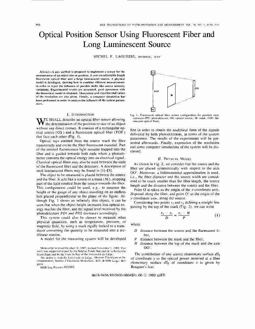
without any direct contact. It consists of a rectangular op- tical source (OS ) and a fluorescent optical fiber (FOF ) that face each other (Fig. 1 ) .

Optical rays emitted from the source reach the fiber transversely and excite the fiber fluorescent material. Part of the emitted fluorescence light remains trapped into the fiber and is guided towards both ends where a photode- tector converts the optical energy into an electrical signal. Classical optical fibers may also be used between the ends of the fluorescent fiber and the detectors. A description of such luminescent fibers may be found in [ 11-[3].

The object to be measured is placed between the source and the fiber. It acts like a screen or a mask ( M ) , stopping part of the light emitted from the source towards the fiber. This configuration could be used, e.g., to measure the height or the gauge of any object traveling on an endless belt placed perpendicular to the plane of the figure. Al- though Fig. l shows an infinitely thin object, it can be seen that when the object height increases less optical en- ergy reaches the fiber, and the signal level received by the photodetectors PD1 and PD2 decreases accordingly.

This system could also be chosen to measure other physical quantities, such as temperature. pressure, or magnetic field, by using a mask rigidly locked to a trans- ducer converting the quantity to be measured into a rec- tilinear motion.

A model for the measuring system will be developed

Manuscript received October 12, 1987; revised November 7. 1988. This work was supported in part by the Belgian Fonds National de la Recherche Scientifique and by the Legs de Bay of the Universite de Liege.

The author is with the Univeraite de Li>gr, Meaures Electriques et In- strumentation. Institut d’Electricite Montcfiore, B2X. B-4000 Liege, Bel- gium.

IEEE Log Number 8926905.

U

Fig. 1 . Fluorescent optical fiber sensor configuration for position mea- surement (PD: photodetector, OS: optical source, M: mask, FOF: flu- orescent optical fiber).

first in order to obtain the analytical form of the signals delivered by both photodetectors, in terms of the system parameters. The results of the experiments will be pre- sented afterwards. Finally, expression of the resolution and some computer simulations of the system will be dis- cussed.

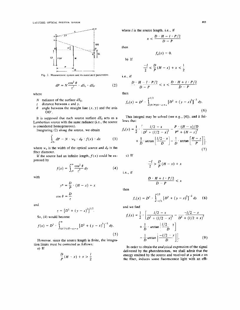
11. PHYSICAL MODEL As shown in Fig. 2, we consider that the source and the

fiber are placed symmetrically with respect to the axis 00’. Moreover, a bidimensional approximation is used, i.e., the fiber diameter and the source width are consid- ered to be much smaller than the fiber length, the source length and the distance between the source and the fiber.

Point 0 is taken as the origin of the x-coordinate axis, disposed along the fiber, and point 0’ as the origin of the y-coordinate axis, along the source.

Considering two points x , and yI defining a straight line passing by the top of the mask (Fig. 2), we can write

where

D distance between the source and the fluorescent fi-

P distance between the mask and the fiber, H distance between the top of the mask and the axis

The contribution of any source elementary surface dSs of coordinate y to the optical power received at a fiber elementary surface dSF of coordinate x is given by Bouguer’s law:

ber,

00‘.

0018-9456/89/0600-0804$01 .OO 0 1989 IEEE

LAGUESSE: OPTICAL POSITION SENSOR 805

where 1 is the source length, i.e., if

D . H - 1 * P / 2 D - P

x <

then

f a ( . ) = 0.

b) If

Fig. 2 . Measurement system and its associated parameters

cos2 8 dP = N - * dSs * dsF

Z2

where

N radiance of the surface dSs, z distance between x and y , 0 angle between the straight line ( x , y ) and the axis

It is supposed that each source surface dSs acts as a Lambertian source with the same radiance (i.e., the source is considered homogeneous).

00’.

Integrating (2) along the source, we obtain

dP = N * ws * dF * f ( x ) * dx ( 3 ) s, where ws is the width of the optical source and dF is the fiber diameter.

If the source had an infinite length, f ( x ) could be ex- pressed by

m cos2 8 dY

with

( H - X) + x D

’ * = P a D

COS 8 = - 2

and 2 I / ’ . z = [D2 + ( y - X) ]

So, (4) would become m

f ( x ) = D2 * j [D2 + ( y - x,’]-’ dy. ( D / P ) ( H - x ) + X

(4)

( 5 ) However, since the source length is finite, the integra-

a) If tion limits must be corrected as follows:

D 1 - ( H - X ) + X > - P 2

- 1 D 1 2 P 2

- < - ( ( H - x ) + x < -

i.e., if

D H - 1 * P / 2 D * H + l * P / 2 < x <

D - P D - P

then

( 6 ) This integral may be solved (see e.g. , [4]), and it fol-

lows that:

P * ( H - x ) / D f b ( x ) = 2 [D’ + ( 1 / 2 - x)’ P2 + ( H - X?

- 1 1/2 - x

1 1 / 2 - x 1 + D - - arctan [ 7 1 - D - arctan [ 7 I]. (7)

c) If

-1 D - > - ( H - x ) + x 2 P

i.e., if

D . H + 1 * P / 2 D - P

< X

then

and we find

-1 /2 - x - 1 1/2 - x

”(‘) = 5 * [D’ + ( 1 / 2 - x,’ D2 + ( 1 / 2 + X?

1 1/2 -

1 -1 /2 - x

+ - D - arctan [+] - - arctan [ 11.

D ( 9 )

In order to obtain the analytical expression of the signal delivered by the photodetectors, we shall admit that the energy emitted by the source and received at a point x on the fiber, induces some fluorescence light with an effi-

806 IEEE TRANSACTIONS ON INSTRUMENTATION A N D MEASUREMENT, VOL. 38. NO. 3. JUNE 1989

ciency qa. Only a fraction qb of this fluorescence energy is emitted in the acceptance cone of the fiber. The energy received at PD1 can be obtained by summing all the ele- mentary fluorescence energies emitted at each point x . We must, therefore, integrate expressions (7) and (9), but also take into account the intensity attenuation of the light guided in the fiber. We shall consider, in a first approxi- mation, that, for PD1, this attenuation may be modeled by an exponential like

p ( L / 2 + x )

where L is length of the fluorescent fiber and CY is the fiber attenuation coefficient.

Consequently, the signal delivered by PD1 may be written as

( 1 0 ) where qc is the fraction of the guided fluorescence light which travels towards PD1; C 1 is a factor representing: 1 ) the attenuation introduced by a classical fiber eventu- ally used to connect the end of the fluorescent fiber to the photodetector and 2 ) the coupling losses between the fiber and PD1, and RI is the radiant sensitivity of PD1:

D . H - l . P / 2 - L ( D - P 'I) bil = max

D * H + 1 - P / 2 L ( D - P ' 2 ) bsl = min

D . H + I . P / 2 - L ( D - P 'r) biz = max

and

L bs2 = 2.

The coefficients vu , 7 6 , qc, and CY are taken as being constant, whatever the value of x , since the fluorescent fiber is considered to be homogeneous (i.e., with a con- stant dopant concentration).

For PD2, we obtain

I , = N . C Z . R ~ . W S . ~ F . ~ ~ ' ~ ] ~ ' ( ~ - q c )

( 1 1 ) 1 . e - a ( L / 2 - X ) dx

where R, is the sensitivity of PD2 and C2 represents the same effects as coefficient C 1 , but for the second mea- surement channel.

Notice that each of the integrals in (10) and ( 1 1 ) must be taken equal to zero when the lower limit becomes greater than the upper limit.

The constants C 1 , C 2 , R I , R2, vu, v b , and qc may be eliminated by first measuring the signals delivered by the two photodetectors without any mask between the source and the fluorescent fiber. If (10) and ( 1 1 ) are evaluated for H becoming infinitely large and negative, we obtain

I ; = N ' C I ' R I Ws * dF vu * 7 6 ' qc

( 1 2 ) fc(x) . e-Q'(L/*+X) dx - L / 2

r L I 2

Since the source intensity may drift with time, N and

Putting (12) in (10) and (13) in ( 1 1 ) it follows that N' may be different.

f,(x) e-OU dx J -L,2

( 1 5 ) If the source drift is sufficiently small, we can consider

N to be equal to N ' . The expressions (14) and (15) can then be numerically evaluated. Otherwise, a reference channel must be used. This third measurement channel is formed by a small piece of fluorescent fiber placed close to the source and delivering a signal Z3 proportional to the source intensity:

1 3 = N . K ( 1 6 )

I ; = N' * K . ( 1 7 )

and without mask:

Combining (14)-(17) , it follows that

f c ( x ) . e-"dx J - L / 2

LAGUESSE. OPTICAL POSITION SENSOR 807

Another method may be used to reject the source inten- sity drifts. In fact, if we combine (14) and ( 1 3 , we obtain

II / I ,

(20) This expression is seen to be independent of any source

intensity variations and does not require any additional channel.

111. EXPERIMENTAL SETUP The fluorescent fiber has initially been developed by the

STIPE at the Centre d'Etudes Nucleaires (CEN) Saclay, France; it is now commercialized by the French company Optectron. We used a doped polystyrene optical fiber PLASTIFO F201 with a diameter of 1 mm. This fiber presents an exitation maximum near 450 nm and an emis- sion maximum near 500 nm. The source is a LUCANYA electroluminescent device from SINEL. Experimental measurements have been made with two sources of dif- ferent size: 97 mm x 14 mm and 280 mm X 11 mm. We chose a "green aviation"-type source. Powered with a 400-Hz alternative tension, it delivers a green color light. However, we have noticed that when a tension of a few kilohertz was applied, the emission wavelength was de- creasing and a blue light could be obtained. During our measurements, we used a 2.8 kHz . 120 V, rms sinu- soidal tension. We have observed that the emitted light had a color such that the fiber fluorescence was excited with good efficiency. Moreover, the source light had the property to be intensity modulated with an important spectral component at a frequency equal to twice the sup- ply frequency.

Classical 1 -mm PMMA optical fibers were also used to connect each end of the fluorescent fiber to a reverse- biased p-i-n photodiode. Each diode was followed by a selective ac amplifier tuned on 5.6 kHz in order to reject the influence of ambient light, and followed itself by an active rectifier and a low-pass filter. The signals delivered by the measurement channels were analyzed by a micro- computer which controlled an analog scanner and a dc voltmeter with an IEEE-488 interface. An automatic sys- tem was used to position the mask between the source and the fluorescent fiber.

As explained above, a reference channel was also im- plemented since we noticed the presence of a small source intensity drift.

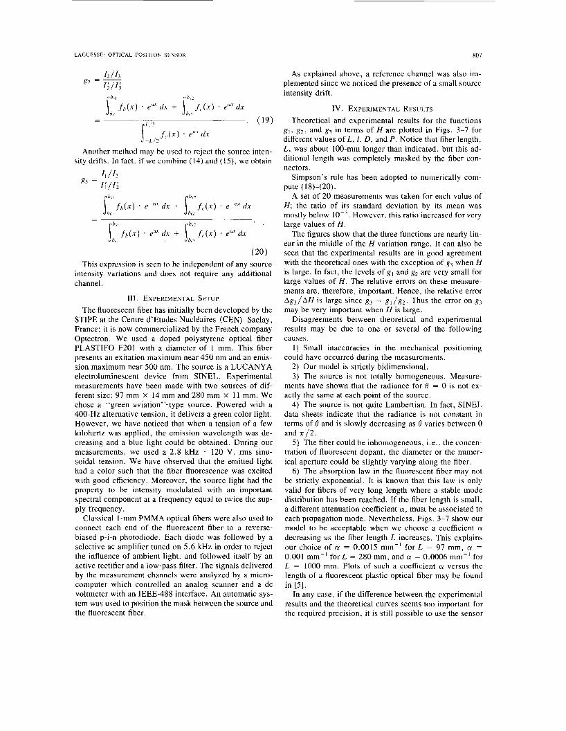
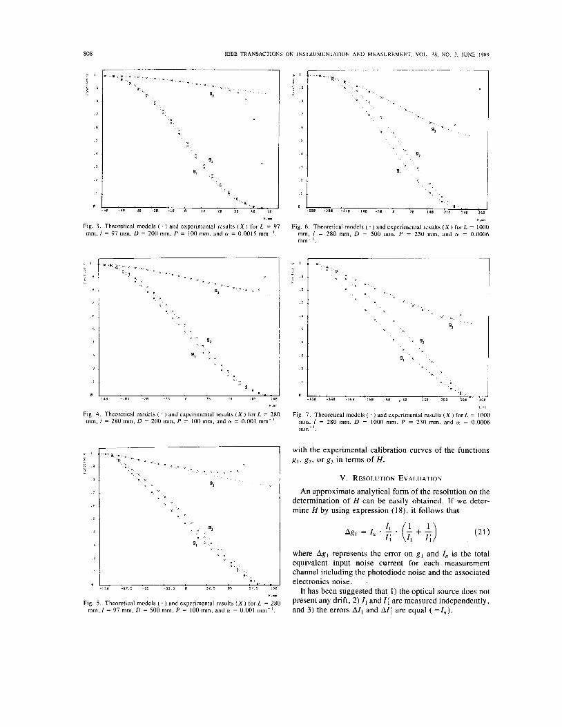
IV. EXPERIMENTAL RESULTS Theoretical and experimental results for the functions

g l , g 2 , and g3 in terms of H are plotted in Figs. 3-7 for different values of I,, I, D, and P . Notice that fiber length, L , was about 100-mm longer than indicated, but this ad- ditional length was completely masked by the fiber con- nectors.

Simpson's rule has been adopted to numerically com- pute ( I 8)-(20).

A set of 20 measurements was taken for each value of H ; the ratio of its standard deviation by its mean was mostly below However, this ratio increased for very large values of H .

The figures show that the three functions are nearly lin- ear in the middle of the H variation range. It can also be seen that the experimental results are in good agreement with the theoretical ones with the exception of g3 when H is large. In fact, the levels of g l and g 2 are very small for large values of H . The relative errors on these measure- ments are, therefore, important. Hence, the relative error A g 3 / A H is large since g, = gl /g2 . Thus the error on g3 may be very important when H is large.

Disagreements between theoretical and experimental results may be due to one or several of the following causes.

1) Small inaccuracies in the mechanical positioning could have occurred during the measurements.

2) Our model is strictly bidimensional. 3) The source is not totally homogeneous. Measure-

ments have shown that the radiance for 8 = 0 is not ex- actly the same at each point of the source.

4) The source is not quite Lambertian. In fact, SINEL data sheets indicate that the radiance is not constant in terms of 8 and is slowly decreasing as 8 varies between 0 and ~ / 2 .

5) The fiber could be inhomogeneous, i .e. , the concen- tration of fluorescent dopant, the diameter or the numer- ical aperture could be slightly varying along the fiber.

6) The absorption law in the fluorescent fiber may not be strictly exponential. It is known that this law is only valid for fibers of very long length where a stable mode distribution has been reached. If the fiber length is small, a different attenuation coefficient CY, must be associated to each propagation mode. Nevertheless, Figs. 3-7 show our model to be acceptable when we choose a coefficient (Y

decreasing as the fiber length L increases. This explains our choice of CY = 0.0015 mm-l for L = 97 mm, (Y = 0.001 mm-' for L = 280 mm, and CY = 0.0006 mm-' for L = 1000 mm. Plots of such a coefficient (Y versus the length of a fluorescent plastic optical fiber may be found in [5].

In any case, if the difference between the experimental results and the theoretical curves seems too important for the required precision, it is still possible to use the sensor

808

a 1

t .9

E

7

6

5

4

3

2

1

B

IEEE TRANSACTIONS ON INSTRUMENTATION AND MEASUREMENT, VOL. 38, NO. 3, JUNE 1989

- 3 0 -48 - 3 8 - 2 8 - 1 8 8 18 28 30 4 8 58

H.rn

Fig. 3 . Theoretical models ( . ) and experimental results ( X ) for L = 97 mm, I = 97 mm, D = 200 mm, P = 100 mm, and a = 0.0015 mm- ' .

m l

: . 9 !

8

7

6

5

4

3

2

1

8

1

48 -185 - 7 0 - 3 5 0 3 5 72 . e 5 : I 8

".%-

Fig. 4. Theoretical models ( . ) and experimental results ( X ) for L = 2180 mm, I = 280 mm, D = 200 mm. P = 100 mm. and a = 0.001 mm- .

I x 9 2 I

B J... . - -138 - 9 7 . 5 - 6 5 - 3 2 . 5 8 3 2 . 5 65 9 7 . 5 138

H.mm

Fig. 5 . Theoretical models ( . ) and experimental results ( X ) for L = 280 mm, I = 97 mm, D = 500 mm, P = 100 mm, and 01 = 0.001 mm- ' .

0 . 1

< . 9 3

B

7

6

5

I

3

2

I

0

.. X .

x . .

a ...

'* x

9, '. ' .

H . N T

Fig. 6 . Theoretical models ( . ) and experimental results ( X ) for L = 1000 mm, I = 280 mm, D = 500 mm, P = 250 mm, and a = 0.0006 mm- '

i I

: . 5

E

7

6

5

4

3

2

8

x x

, * 5 8 -358 - 2 5 8 - 1 5 8 -58 . 5 8 158 2 5 0 3 5 0 158

H.mm

Fig. 7 . Theoretical models ( . ) and experimental results ( X ) forL = 1000 mm. I = 280 mm, D = 1000 mm, P = 230 mm, and a = 0.0006 m m - I .

with the experimental calibration curves of the functions g , , g 2 , or g3 in terms of H.

V . RESOLUTION EVALUATION

An approximate analytical form of the resolution on the determination of H can be easily obtained. If we deter- mine H by using expression (18), it follows that

where Ag] represents the error on g, and I,, is the total equivalent input noise current for each measurement channel including the photodiode noise and the associated electronics noise.

It has been suggested that 1) the optical source does not present any drift, 2) I, and Z are measured independently, and 3) the errors AZ, and AZ; are equal ( =I,).

LAGUESSE: OPTICAL POSITION SENSOR

6 .

5

I .

3

2

1 .

In order to obtain A H , we must introduce the derivative of g , with respect to H :

a, . .

a, ' .

1 . : . . . . . .

809

I

3 .

2 .

I

Finally, we may write

1, - 1

A H = [ % ] . . _ cl ' w S ' dF . q a ' l?b q r

..

..

bsz

+ be 2 f c ( x ) * C U d x ] . (23)

This expression clearly shows how the resolution could be improved, e.g. , by decreasing the noise I , or by in- creasing the coupling coefficients C , , the detector sensi- tivity, the source width, the fiber diameter, the efficiency coefficients qa and q b , or the source intensity.

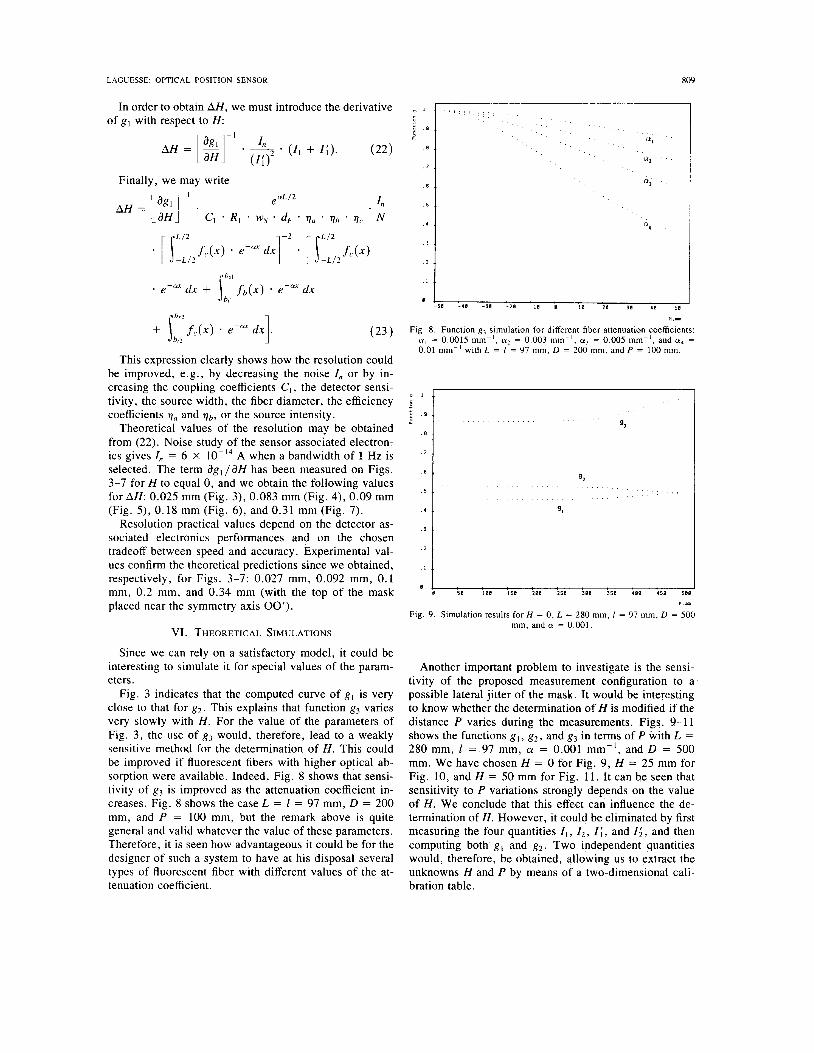
Theoretical values of the resolution may be obtained from (22). Noise study of the sensor associated electron- ics gives I , = 6 X A when a bandwidth of 1 Hz is selected. The term d g , / a H has been measured on Figs. 3-7 for H to equal 0, and we obtain the following values for A H : 0.025 mm (Fig. 3), 0.083 mm (Fig. 4), 0.09 mm (Fig. 5 ) , 0.18 mm (Fig. 6), and 0.31 mm (Fig. 7).

Resolution practical values depend on the detector as- sociated electronics performances and on the chosen tradeoff between speed and accuracy. Experimental val- ues confirm the theoretical predictions since we obtained, respectively, for Figs. 3-7: 0.027 mm, 0.092 mm, 0.1 mm, 0.2 mm, and 0.34 mm (with the top of the mask placed near the symmetry axis 00').

VI. THEORETICAL SIMULATIONS

Since we can rely on a satisfactory model, it could be interesting to simulate it for special values of the param- eters.

Fig. 3 indicates that the computed curve of g , is very close to that for g 2 . This explains that function g 3 varies very slowly with H . For the value of the parameters of Fig. 3, the use of g 3 would, therefore, lead to a weakly sensitive method for the determination of H . This could be improved if fluorescent fibers with higher optical ab- sorption were available. Indeed, Fig. 8 shows that sensi- tivity of g 3 is improved as the attenuation coefficient in- creases. Fig. 8 shows the case L = 1 = 97 mm, D = 200 mm, and P = 100 mm, but the remark above is quite general and valid whatever the value of these parameters. Therefore, it is seen how advantageous it could be for the designer of such a system to have at his disposal several types of fluorescent fiber with different values of the at- tenuation coefficient.

. . .

'3

B 1 B 58 188 158 288 258 388 3 5 1 488 I 5 8 SUB

P.UU0

Fig. 9. Simulation results for H = 0, L = 280 mm, 1 = 97 mm, D = 500 mm, and a = 0.001.

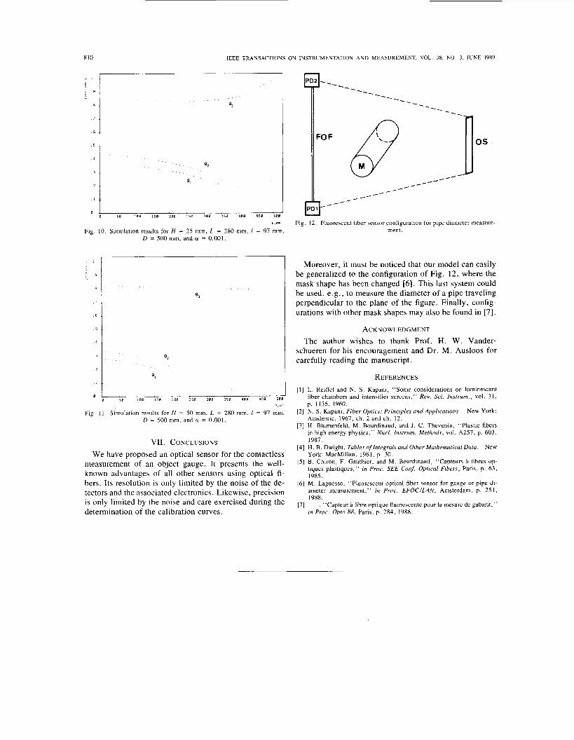
Another important problem to investigate is the sensi- tivity of the proposed measurement configuration to a possible lateral jitter of the mask. It would be interesting to know whether the determination of H is modified if the distance P varies during the measurements. Figs. 9-11 shows the functions g , , g 2 , and g3 in terms of P with L = 280 mm, I = 97 mm, a = 0.001 mm-I, and D = 500 mm. We have chosen H = 0 for Fig. 9, H = 25 mm for Fig. 10, and H = 50 mm for Fig. 11. It can be seen that sensitivity to P variations strongly depends on the value of H . We conclude that this effect can influence the de- termination of H . However, it could be eliminated by first measuring the four quantities I , , Z 2 , I ; , and I ; , and then computing both g , and g 2 . Two independent quantities would, therefore, be obtained, allowing us to extract the unknowns H and P by means of a two-dimensional cali- bration table.

810

? I

5 .9

B

7

6

5

4

3

2

I

0

IEEE TRANSACTIONS ON INSTRUMENTATION AND MEASUREMENT, VOL. 38, NO. 3, JUNE 1989

‘3

92

9,

5 0 1 8 8 158 2 8 8 258 380 358 4 8 8 4 5 8 5 0 8

P.mm

Fig. 10. Simulation results for H = 25 mm, L = 280 mm, I = 97 mm, D = 500 mm, and 01 = 0.001.

I 1

:: 1 4 !

‘3

92 I

I

E 0 58 1 8 8 1 5 8 2 8 8 2 5 0 3 8 0 3 5 0 4 0 8 4 5 8 588

P mm

Fig I 1 Simulation results for H = 50 mm. L = 280 mm, I = 97 mm, D = 500 mm. and CY = 0.001

VII. CONCLUSIONS We have proposed an optical sensor for the contactless

measurement of an object gauge. It presents the well- known advantages of all other sensors using optical fi- bers. Its resolution is only limited by the noise of the de- tectors and the associated electronics. Likewise, precision is only limited by the noise and care exercised during the determination of the calibration curves.

FO F

H-H-- Fig. 12. Fluorescent fiber sensor configuration for pipe diameter measure-

ment.

Moreover, it must be noticed that our model can easily be generalized to the configuration of Fig. 12, where the mask shape has been changed [ 6 ] . This last system could be used, e.g., to measure the diameter of a pipe traveling perpendicular to the plane of the figure. Finally, config- urations with other mask shapes may also be found in [7].

ACKNOWLEDGMENT The author wishes to thank Prof. H. W. Vander-

schueren for his encouragement and Dr. M. Ausloos for carefully reading the manuscript.

REFERENCES [ l ] L. Reiffel and N . S . Kapani, “Some considerations on luminescent

fiber chambers and intensifier screens,” Rev. Sri. Insirurn., vol. 31, p. 1136, 1960.

121 N. S . Kapani, Fiber Optics: Principles and Applicaiions. New York: Academic, 1967, ch. 2 and ch. 12.

[3] H . Blumenfeld, M. Bourdinaud. and J . C. Thevenin, “Plastic fibers in high energy physics,” Nucl. Instrum. Methods, vol. A257, p. 603, 1987.

[4] H. B. Dwight, Tables of Iniegrals and Other Mathematical Data. New York: MacMillan, 1961, p. 30.

[ 5 ] B. Chiron, F. Gauthier, and M. Bourdinaud, “Capteurs ?i fibres op- tiques plastiques,” in Proc. SEE ConJ Optical Fibers, Paris, p. 63. 1985.

[6] M. Laguesse, “Fluorescent optical fiber sensor for gauge or pipe di- ameter measurement,” in Proc. EFOCILAN, Amsterdam, p. 251, 1988.

[7] -, “Capteur i fibre optique fluorescente pour la mesure de gabarit,” in Proc. Opto 88, Paris, p. 284, 1988.