Embed Size (px)
Citation preview

Optical flow
16-385 Computer VisionSpring 2019, Lecture 21http://www.cs.cmu.edu/~16385/

• Homework 6 has been posted and is due on April 24th. - Any questions about the homework?- How many of you have looked at/started/finished homework 6?
• Wednesday’s office hours will be covered by Yannis at the graphics lounge.
Course announcements

• Quick intro to vision for video.
• Optical flow.
• Constant flow.
• Horn-Schunck flow.
Overview of today’s lecture

Slide credits
Most of these slides were adapted from:
• Kris Kitani (16-385, Spring 2017).
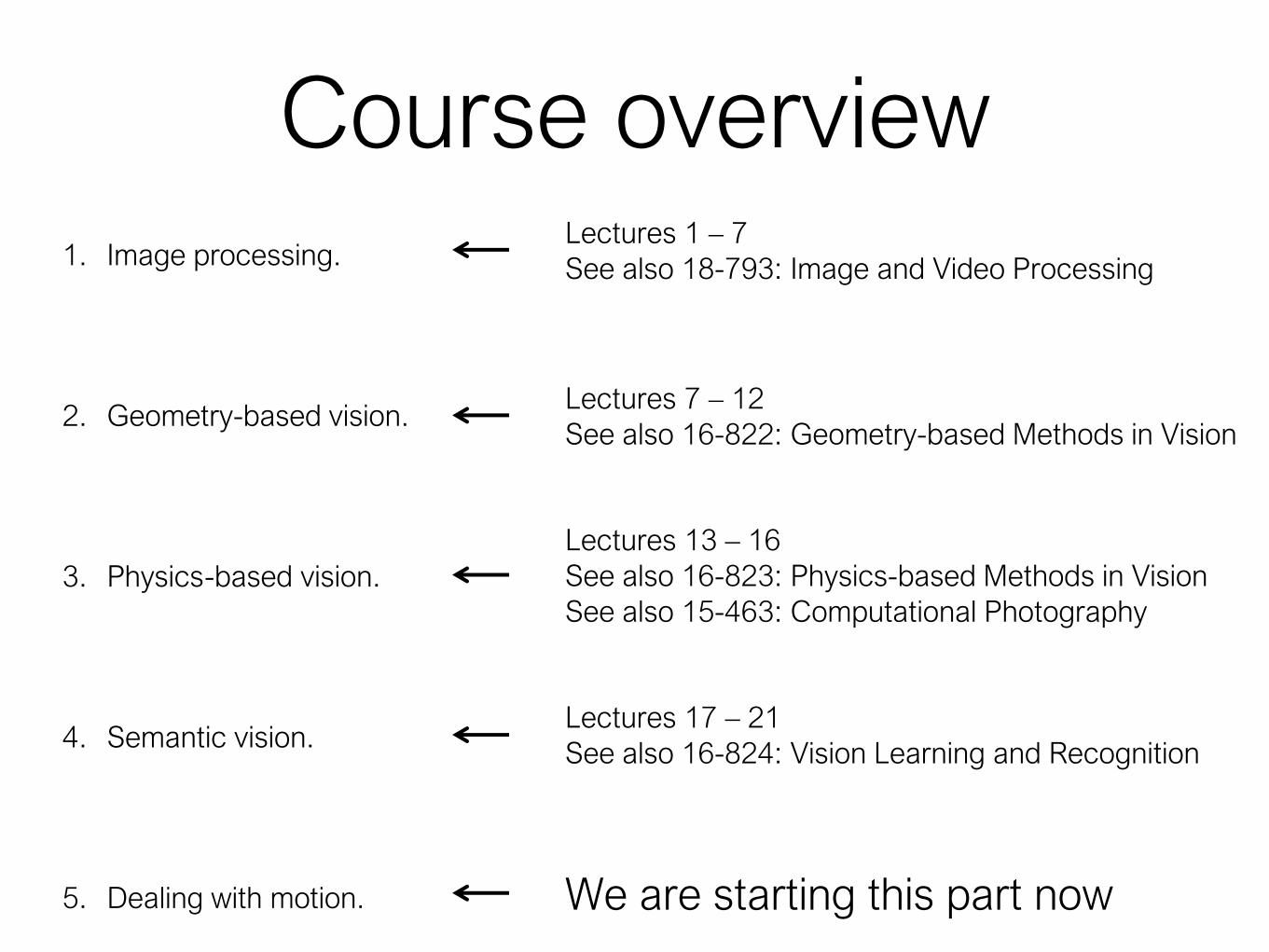
1. Image processing.
2. Geometry-based vision.
3. Physics-based vision.
4. Semantic vision.
5. Dealing with motion.
Course overview
Lectures 13 – 16
See also 16-823: Physics-based Methods in Vision
See also 15-463: Computational Photography
Lectures 7 – 12
See also 16-822: Geometry-based Methods in Vision
Lectures 1 – 7
See also 18-793: Image and Video Processing
We are starting this part now
Lectures 17 – 21
See also 16-824: Vision Learning and Recognition

Computer vision for video

Optical Flow
Constant Flow Horn-Schunck

Optical flow used for feature tracking on a drone

optical flow used for motion estimation in visual odometry

Image Alignment
Lucas-Kanade
(Forward additive)
Baker-Matthews
(Inverse Compositional)

Tracking in Video
KLT Mean shift
Kalman Filtering SLAM
Optical flow
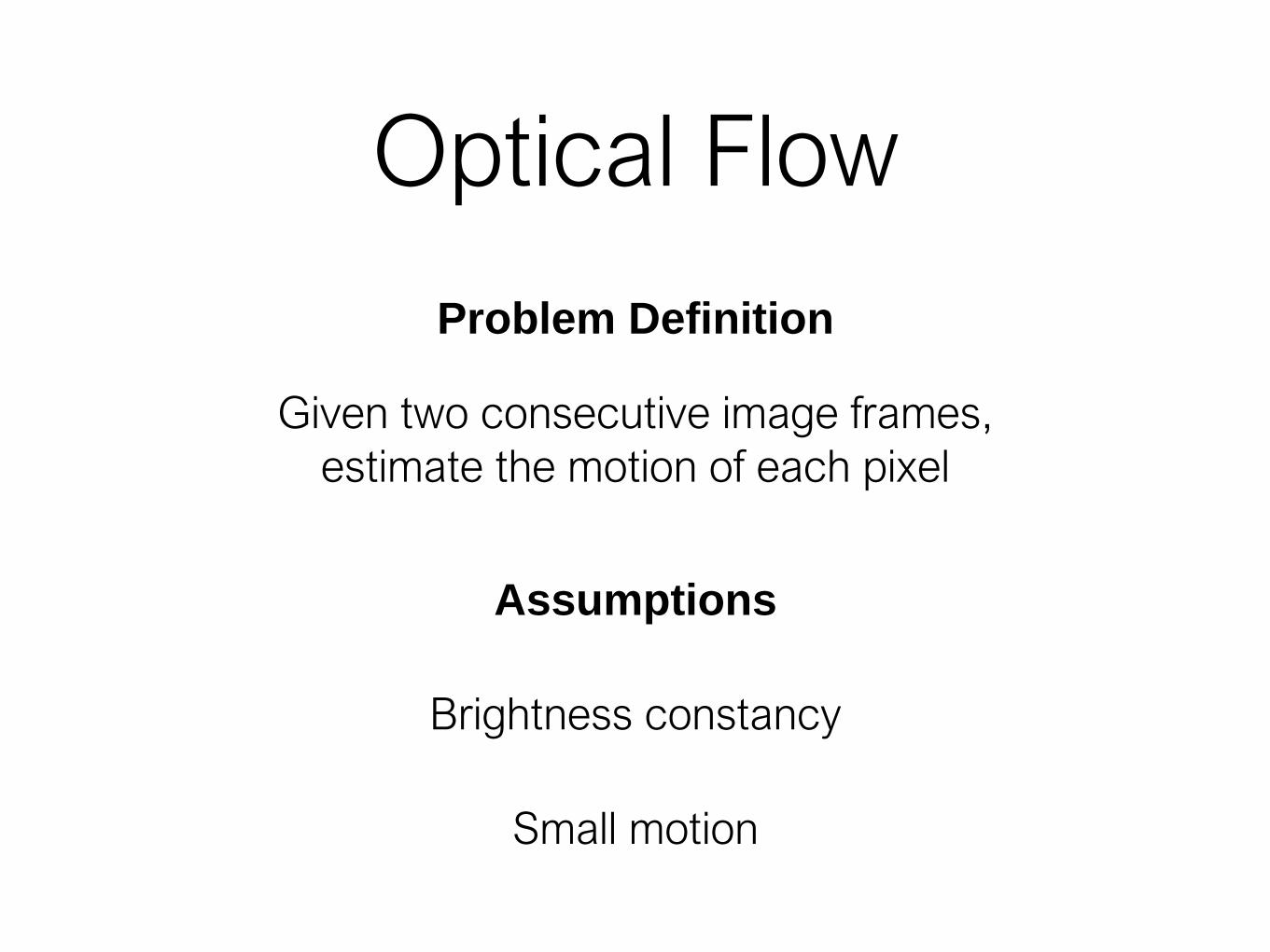
Optical Flow
Problem Definition
Assumptions
Brightness constancy
Small motion
Given two consecutive image frames,
estimate the motion of each pixel
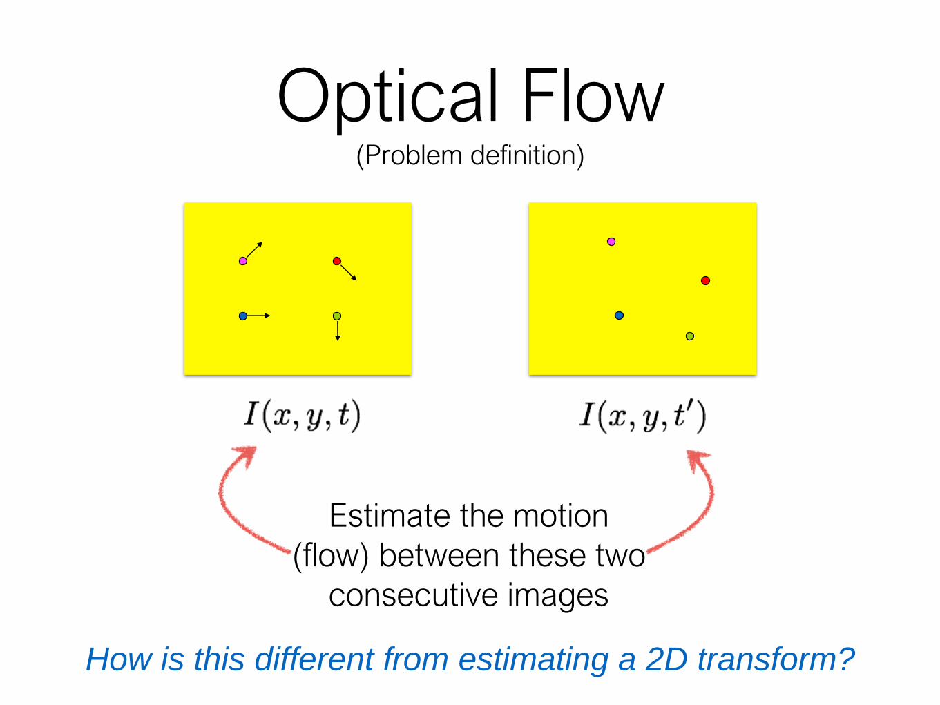
Optical Flow(Problem definition)
Estimate the motion
(flow) between these two
consecutive images
How is this different from estimating a 2D transform?

Key Assumptions(unique to optical flow)
Color Constancy(Brightness constancy for intensity images)
Small Motion(pixels only move a little bit)
Implication: allows for pixel to pixel comparison
(not image features)
Implication: linearization of the brightness
constancy constraint
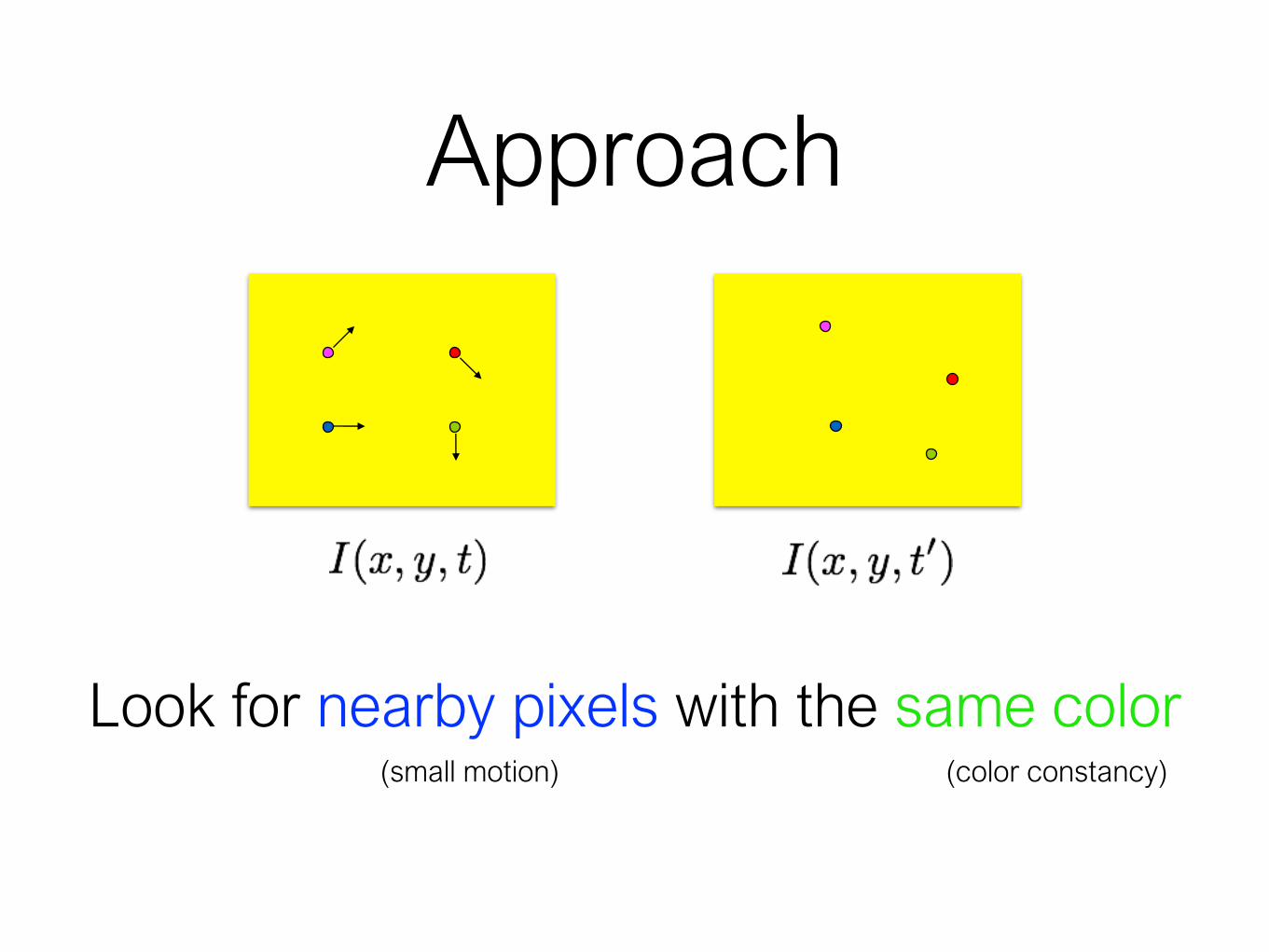
Approach
Look for nearby pixels with the same color(small motion) (color constancy)
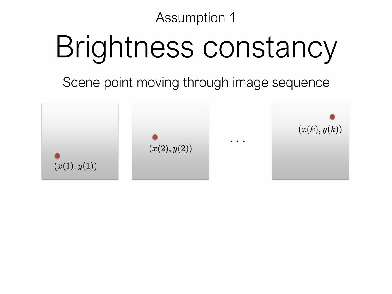
Brightness constancyScene point moving through image sequence
Assumption 1

Brightness constancyScene point moving through image sequence
Assumption 1
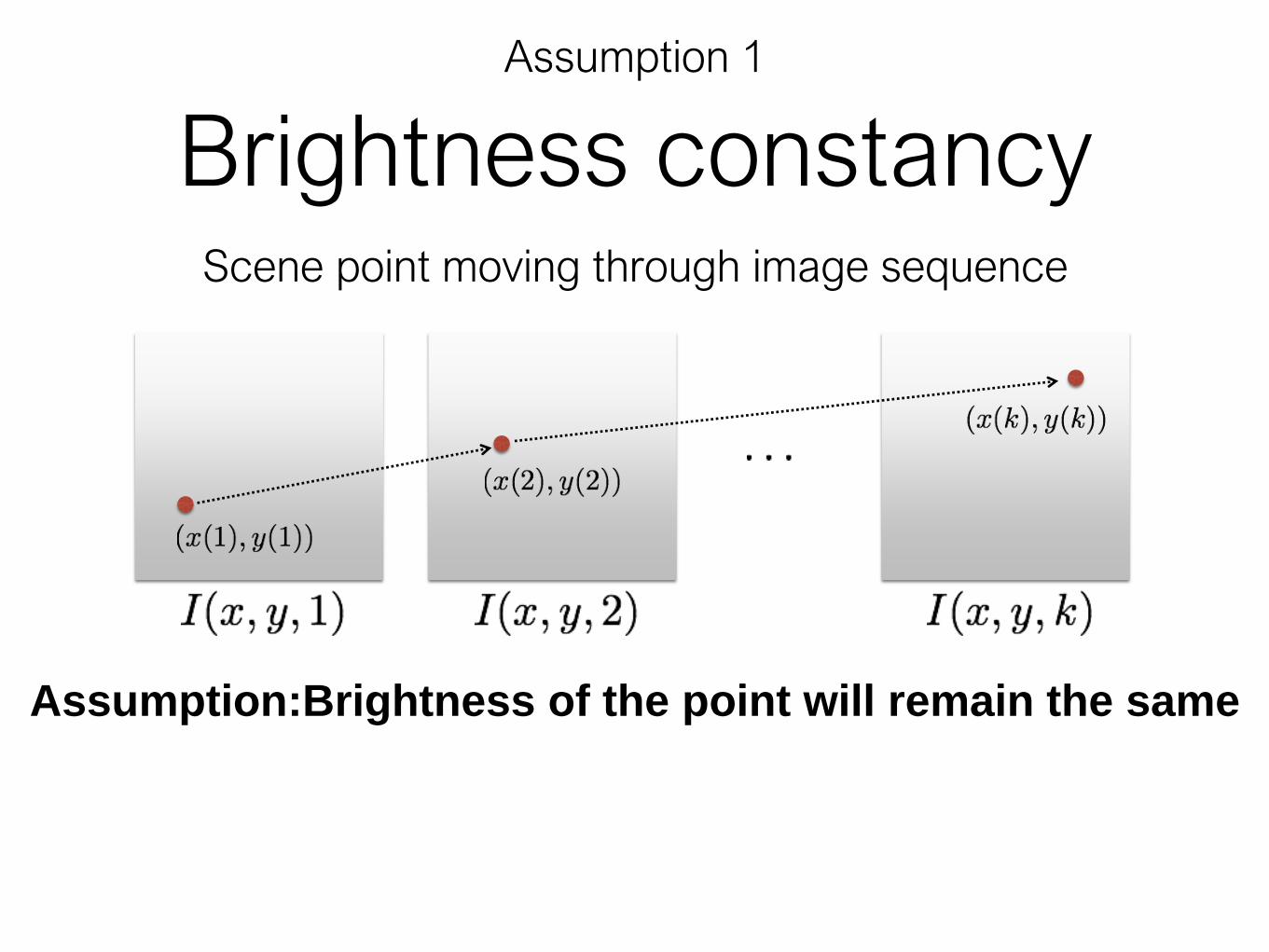
Brightness constancy
Assumption:Brightness of the point will remain the same
Scene point moving through image sequence
Assumption 1
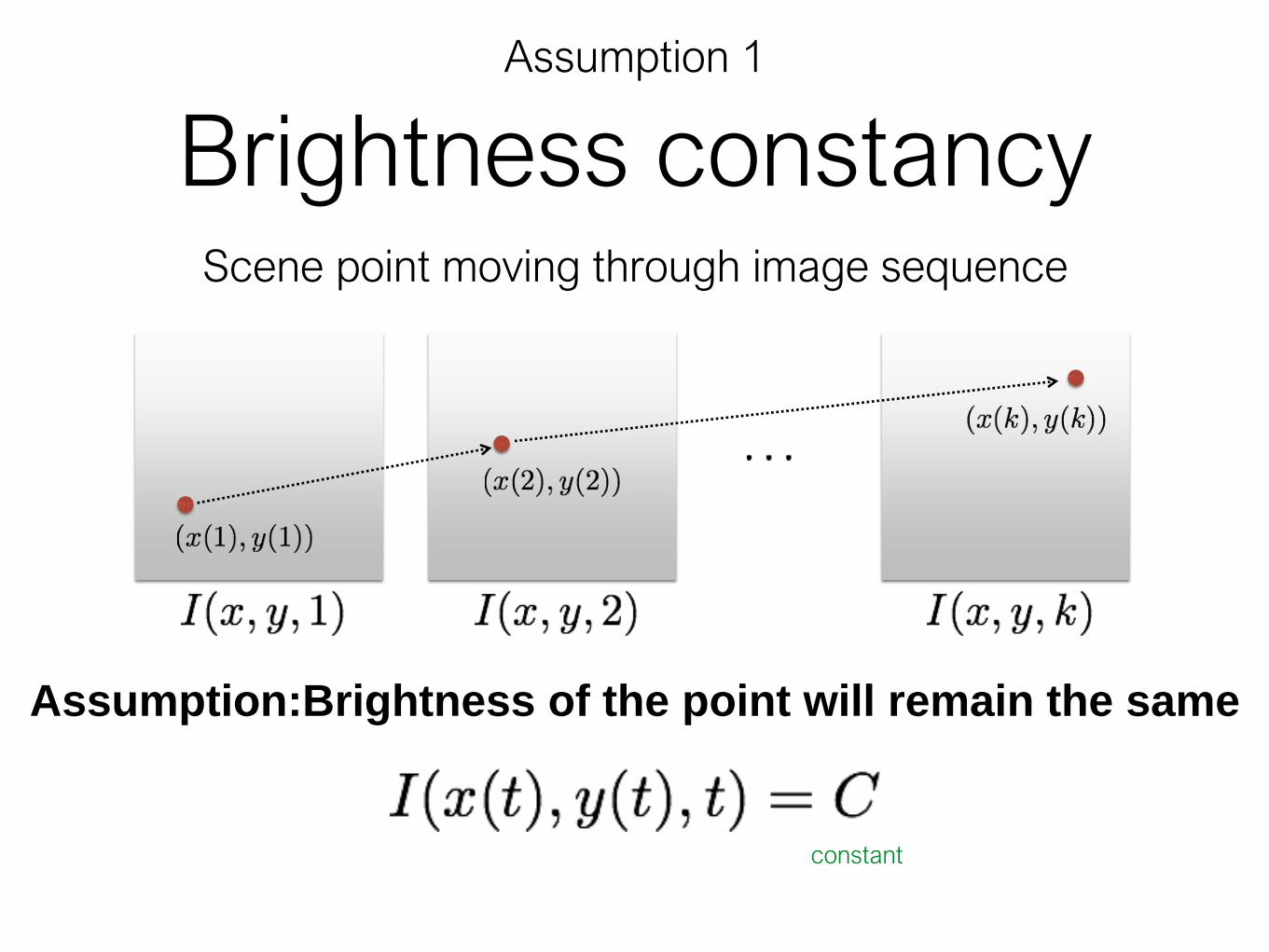
Brightness constancy
Assumption:Brightness of the point will remain the same
constant
Scene point moving through image sequence
Assumption 1

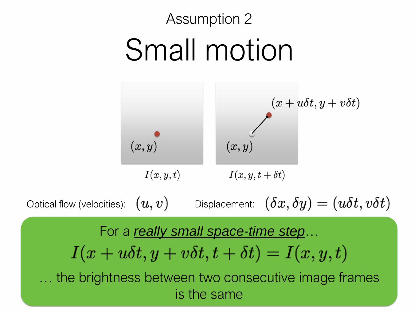
Small motion
Assumption 2

Small motion
Assumption 2

Small motion
Optical flow (velocities): Displacement:
Assumption 2
Small motion
Optical flow (velocities): Displacement:
… the brightness between two consecutive image frames
is the same
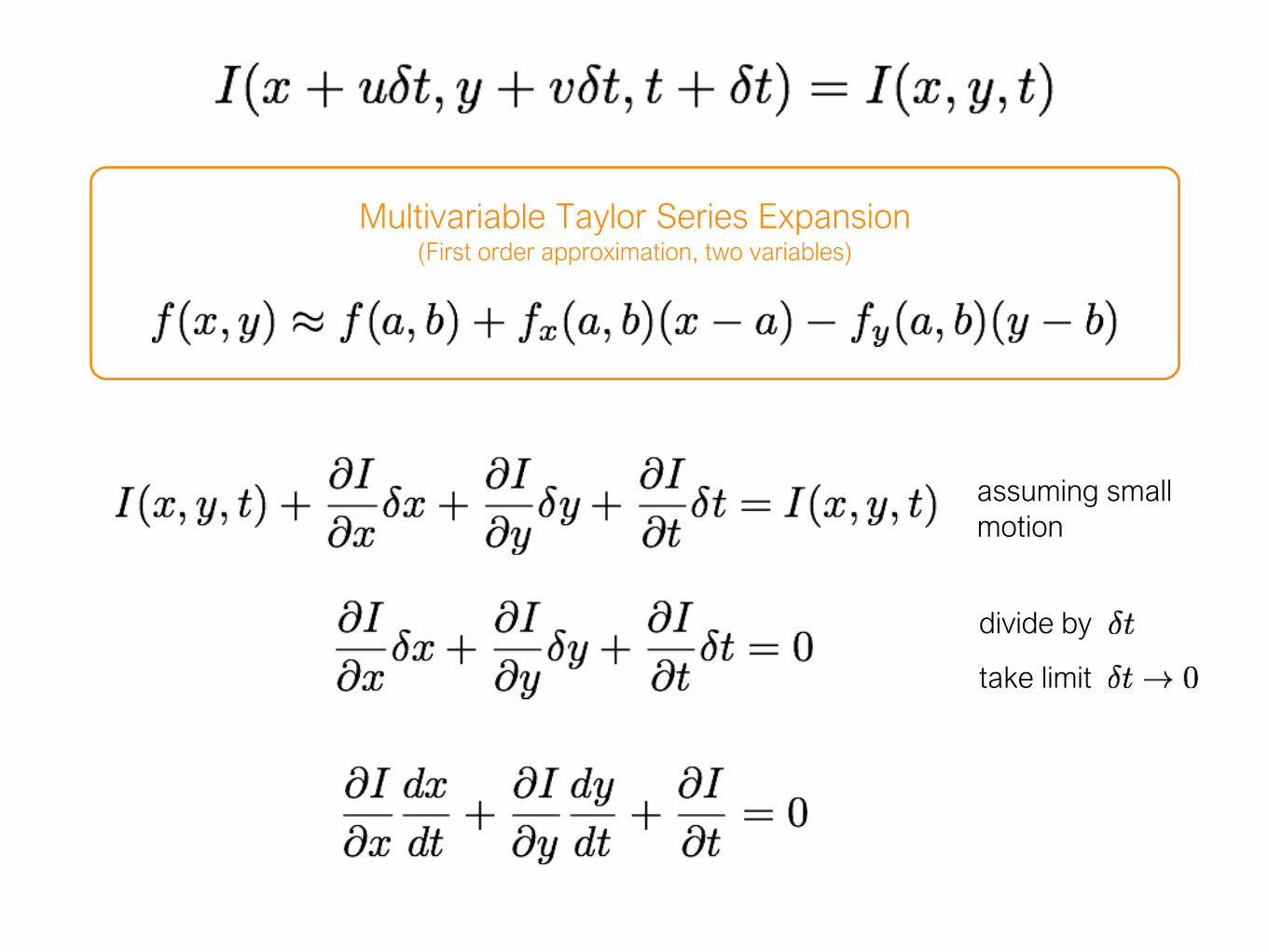
For a really small space-time step…
Assumption 2
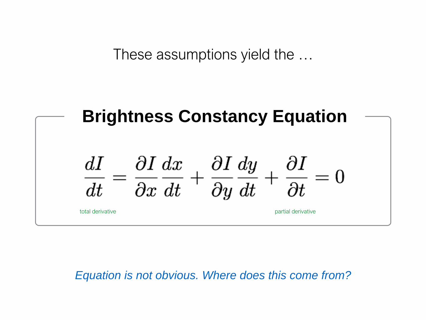
total derivative partial derivative
Equation is not obvious. Where does this come from?
These assumptions yield the …
Brightness Constancy Equation

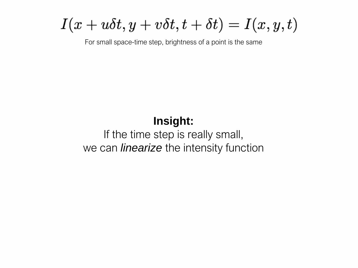
For small space-time step, brightness of a point is the same
For small space-time step, brightness of a point is the same
Insight:
If the time step is really small,
we can linearize the intensity function
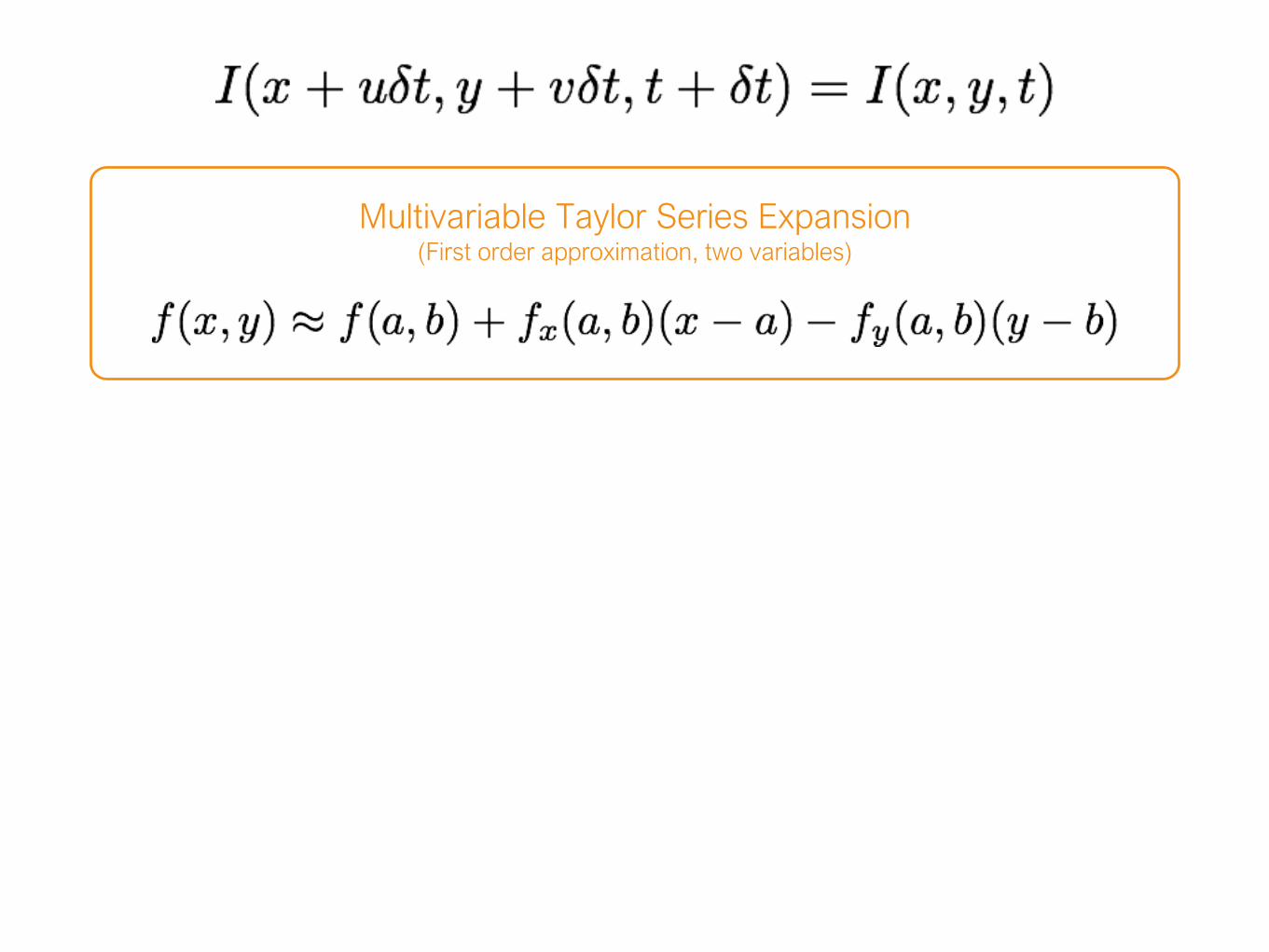
Multivariable Taylor Series Expansion(First order approximation, two variables)

Multivariable Taylor Series Expansion(First order approximation, two variables)
assuming small
motion

assuming small
motion
cancel terms
Multivariable Taylor Series Expansion(First order approximation, two variables)
fixed point
partial derivative

assuming small
motion
cancel terms
Multivariable Taylor Series Expansion(First order approximation, two variables)

assuming small
motion
divide by
take limit
Multivariable Taylor Series Expansion(First order approximation, two variables)
assuming small
motion
divide by
take limit
Multivariable Taylor Series Expansion(First order approximation, two variables)

assuming small
motion
divide by
take limit
Brightness Constancy
Equation
Multivariable Taylor Series Expansion(First order approximation, two variables)
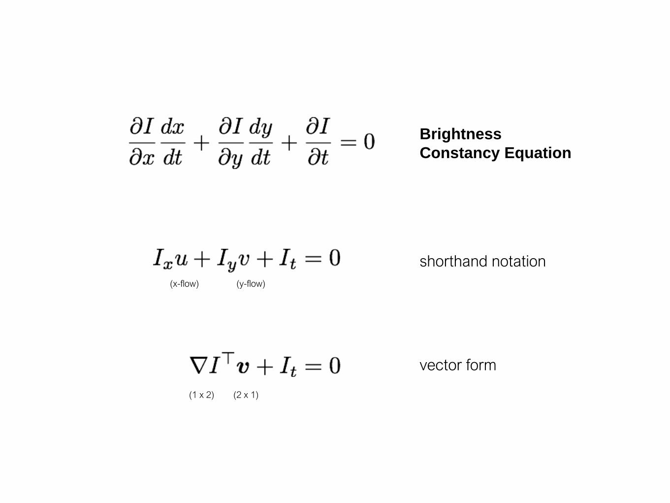
shorthand notation
vector form
Brightness
Constancy Equation
(x-flow) (y-flow)
(1 x 2) (2 x 1)

(putting the math aside for a second…)
What do the term of the
brightness constancy equation represent?

(putting the math aside for a second…)
What do the term of the
brightness constancy equation represent?
Image gradients(at a point p)

(putting the math aside for a second…)
What do the term of the
brightness constancy equation represent?
flow velocities
Image gradients(at a point p)

(putting the math aside for a second…)
What do the term of the
brightness constancy equation represent?
flow velocities
temporal gradient
How do you compute these terms?
Image gradients(at a point p)
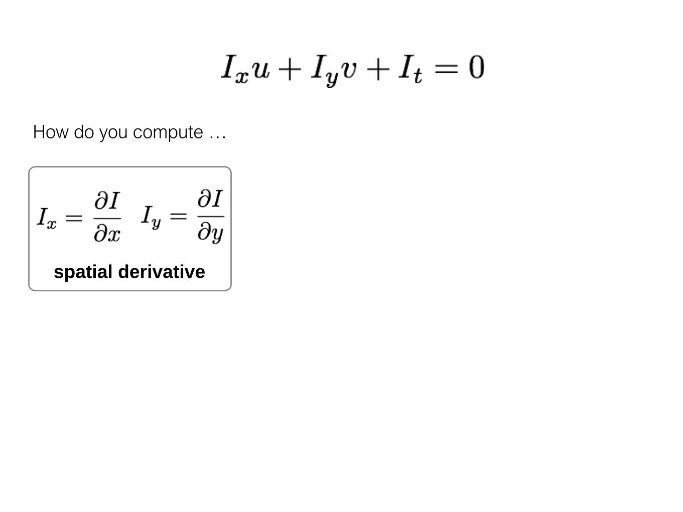
spatial derivative
How do you compute …
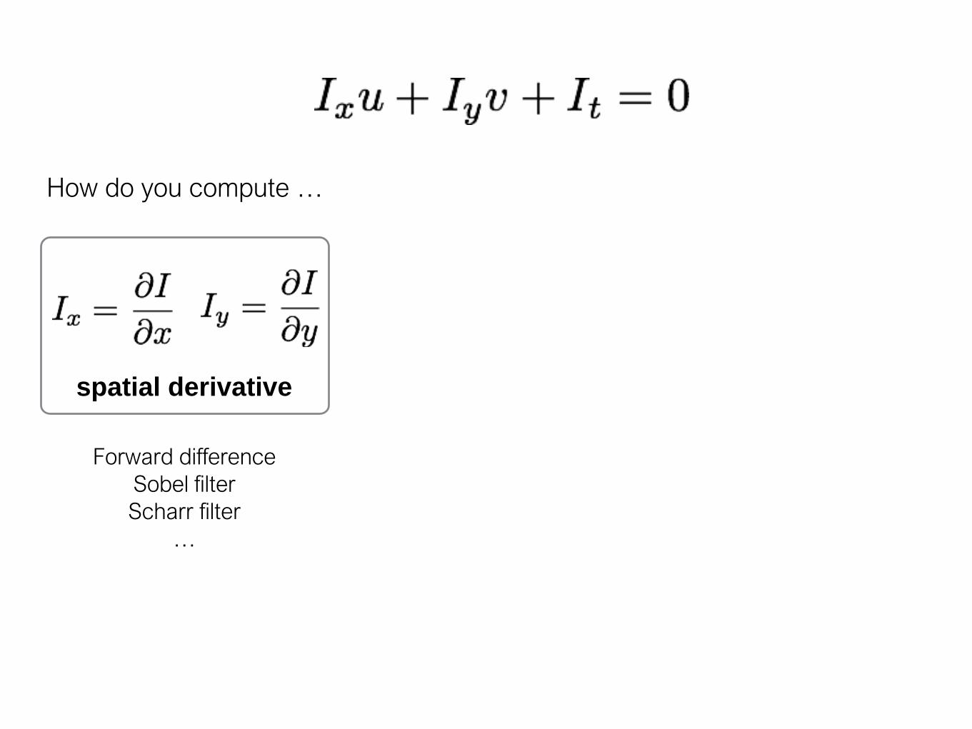
spatial derivative
Forward difference
Sobel filter
Scharr filter
…
How do you compute …
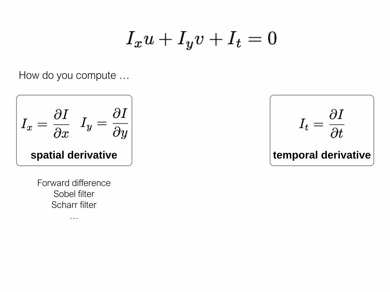
spatial derivative temporal derivative
Forward difference
Sobel filter
Scharr filter
…
How do you compute …

spatial derivative temporal derivative
Forward difference
Sobel filter
Scharr filter
…
How do you compute …
frame differencing

Frame differencing
1 1 1 1 1
1 1 1 1 1
1 10 10 10 10
1 10 10 10 10
1 10 10 10 10
1 10 10 10 10
1 1 1 1 1
1 1 1 1 1
1 1 1 1 1
1 1 10 10 10
1 1 10 10 10
1 1 10 10 10
0 0 0 0 0
0 0 0 0 0
0 9 9 9 9
0 9 0 0 0
0 9 0 0 0
0 9 0 0 0
(example of a forward difference)
- =
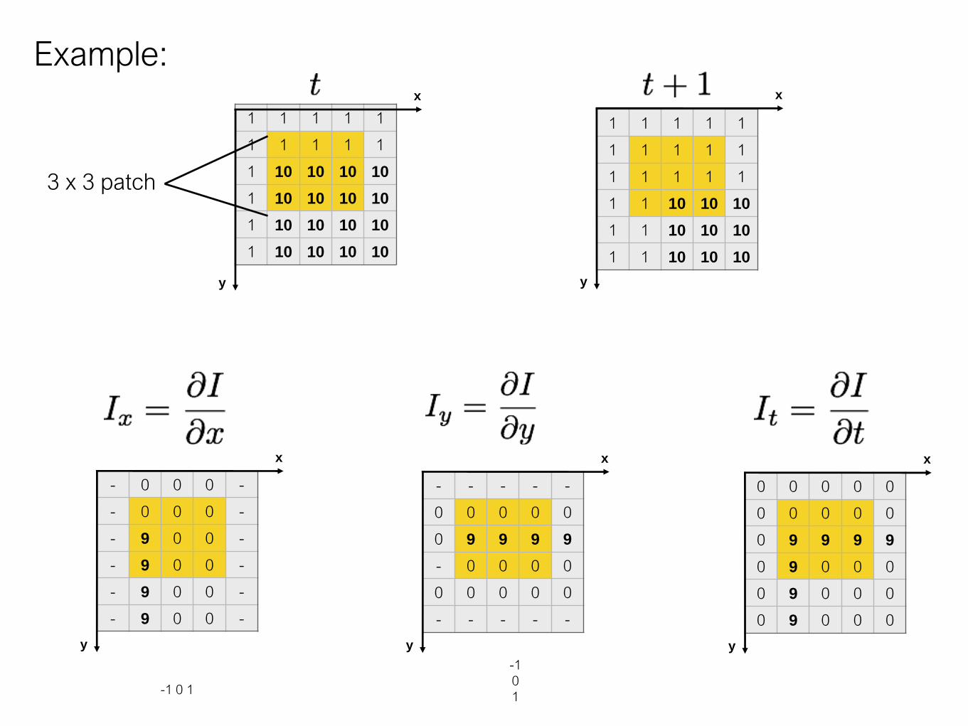
Example:
1 1 1 1 1
1 1 1 1 1
1 10 10 10 10
1 10 10 10 10
1 10 10 10 10
1 10 10 10 10
1 1 1 1 1
1 1 1 1 1
1 1 1 1 1
1 1 10 10 10
1 1 10 10 10
1 1 10 10 10
y
x
y
x
- 0 0 0 -
- 0 0 0 -
- 9 0 0 -
- 9 0 0 -
- 9 0 0 -
- 9 0 0 -
y
x
- - - - -
0 0 0 0 0
0 9 9 9 9
- 0 0 0 0
0 0 0 0 0
- - - - -
y
x
0 0 0 0 0
0 0 0 0 0
0 9 9 9 9
0 9 0 0 0
0 9 0 0 0
0 9 0 0 0
y
x
3 x 3 patch
-1 0 1
-1
0
1
spatial derivative optical flow
Forward difference
Sobel filter
Scharr filter
…
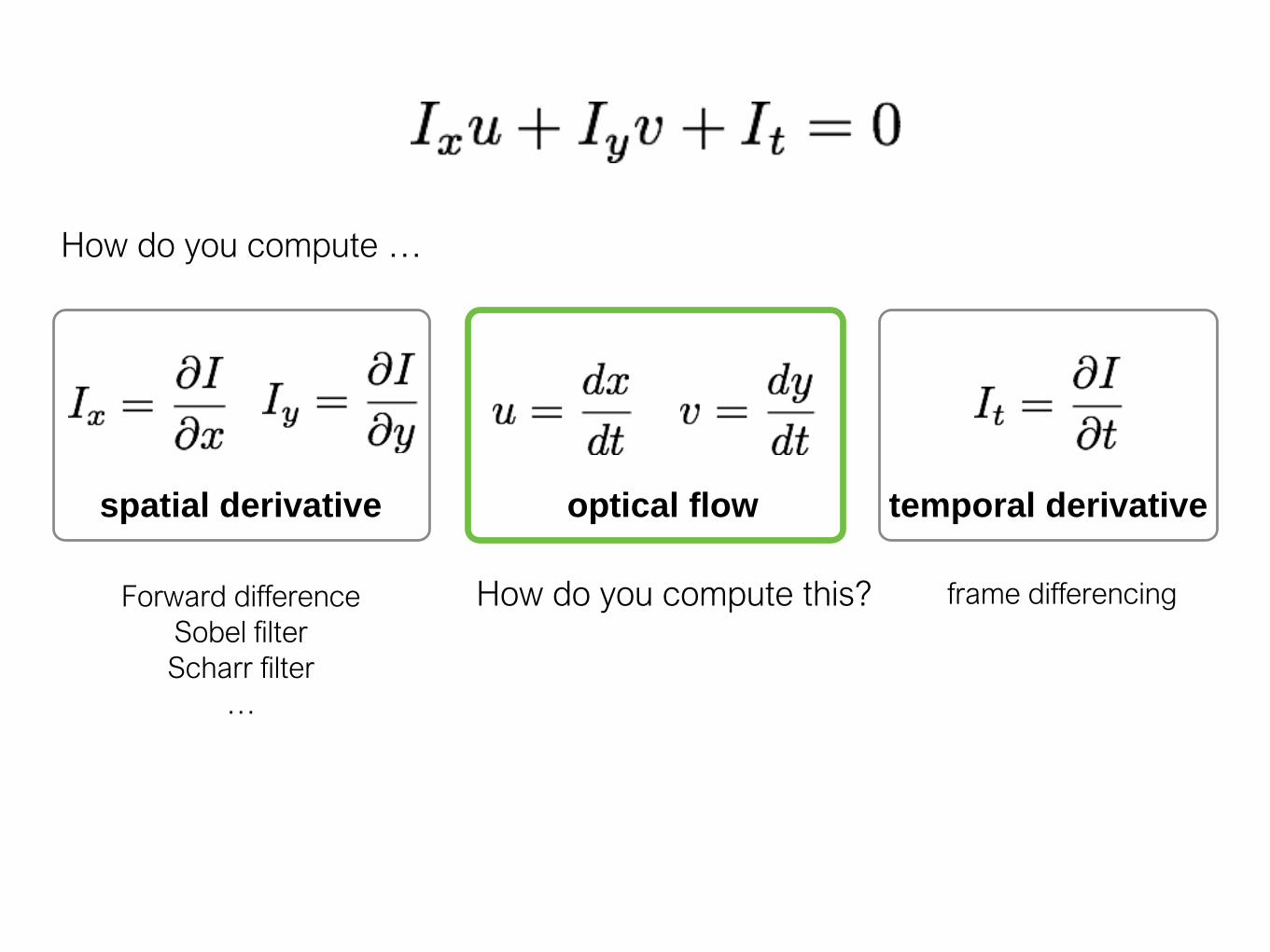
How do you compute …
temporal derivative
frame differencingHow do you compute this?

spatial derivative optical flow
Forward difference
Sobel filter
Scharr filter
…
How do you compute …
temporal derivative
frame differencingWe need to solve for this!(this is the unknown in the optical
flow problem)
spatial derivative optical flow
Forward difference
Sobel filter
Scharr filter
…
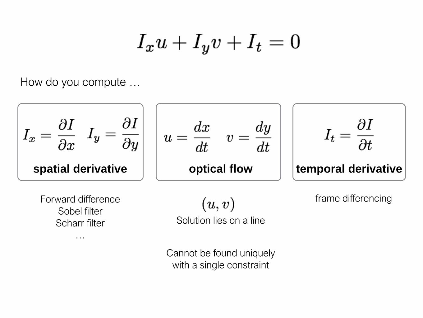
Solution lies on a line
Cannot be found uniquely
with a single constraint
How do you compute …
temporal derivative
frame differencing

Solution lies on a straight line
The solution cannot be determined uniquely with a
single constraint (a single pixel)
many combinations of u and v will satisfy the equality

spatial derivative optical flow temporal derivative
How can we use the brightness constancy equation to
estimate the optical flow?
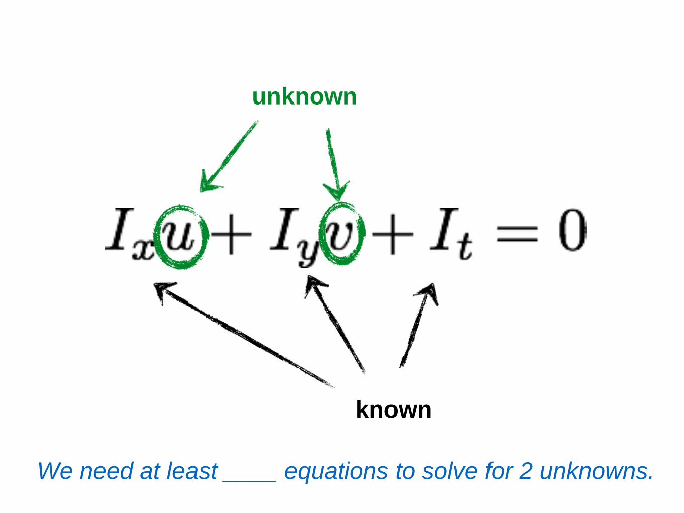
known
unknown
We need at least ____ equations to solve for 2 unknowns.

known
unknown
Where do we get more equations (constraints)?

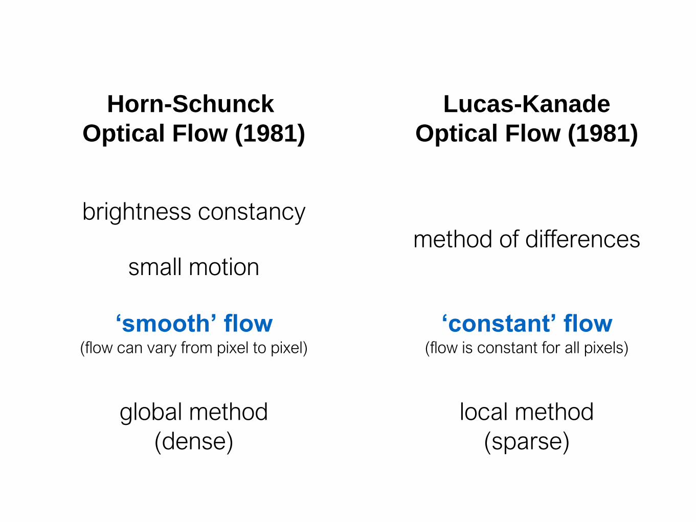
Horn-Schunck
Optical Flow (1981)
Lucas-Kanade
Optical Flow (1981)
‘constant’ flow(flow is constant for all pixels)
‘smooth’ flow(flow can vary from pixel to pixel)
brightness constancymethod of differences
global method
(dense)
local method
(sparse)
small motion

Constant flow
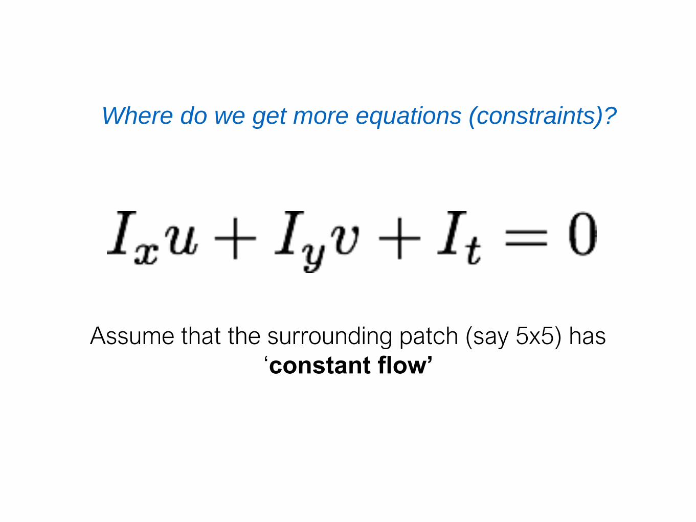
Where do we get more equations (constraints)?
Assume that the surrounding patch (say 5x5) has
‘constant flow’
Flow is locally smooth
Neighboring pixels have same displacement
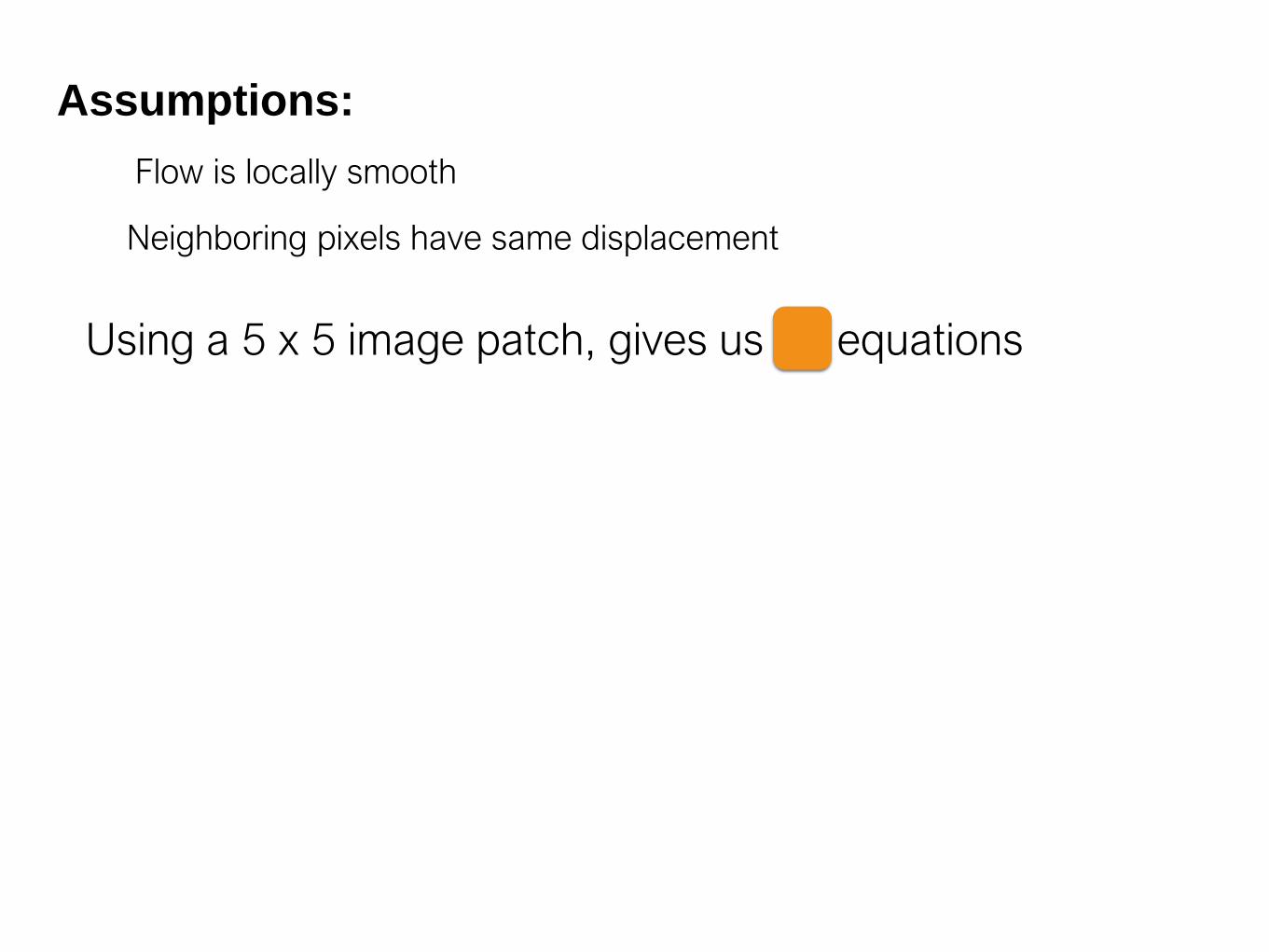
Using a 5 x 5 image patch, gives us 25 equations
Assumptions:

Flow is locally smooth
Neighboring pixels have same displacement
Using a 5 x 5 image patch, gives us 25 equations
Assumptions:
Flow is locally smooth
Neighboring pixels have same displacement
Using a 5 x 5 image patch, gives us 25 equations
Assumptions:
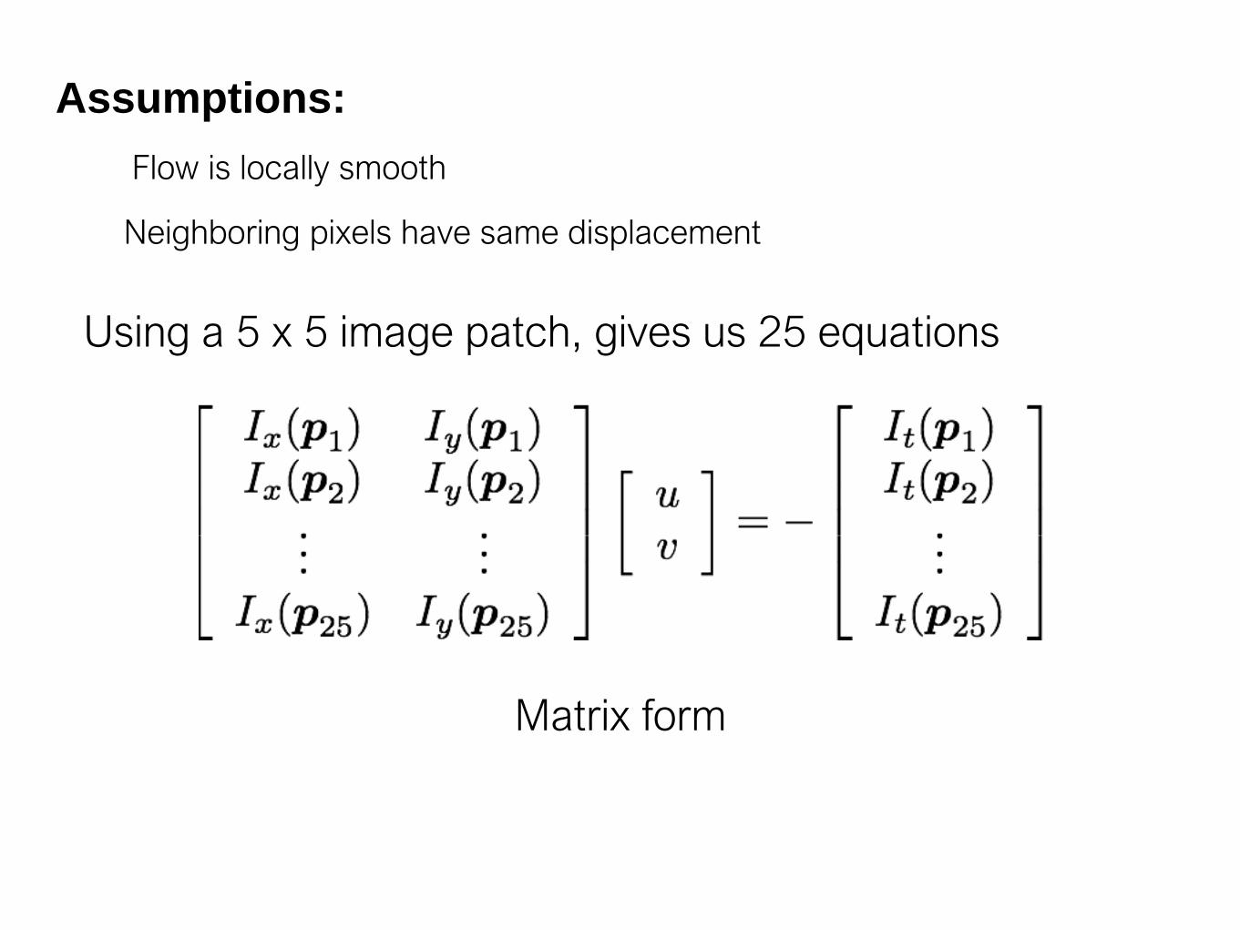
Matrix form

Flow is locally smooth
Neighboring pixels have same displacement
Using a 5 x 5 image patch, gives us 25 equations
How many equations? How many unknowns? How do we solve this?
Assumptions:

Least squares approximation
is equivalent to solving
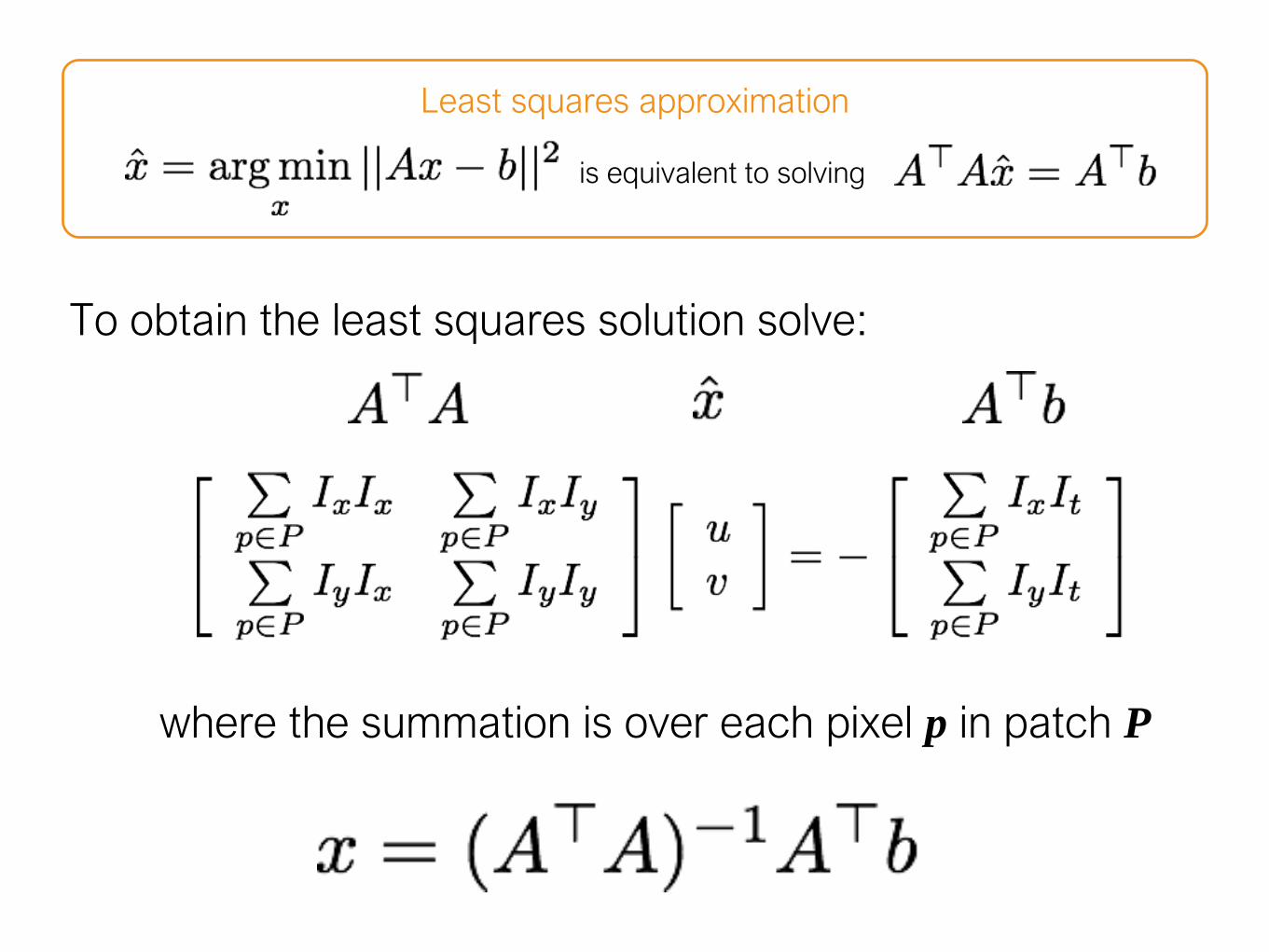
To obtain the least squares solution solve:
Least squares approximation
is equivalent to solving
where the summation is over each pixel p in patch P
To obtain the least squares solution solve:
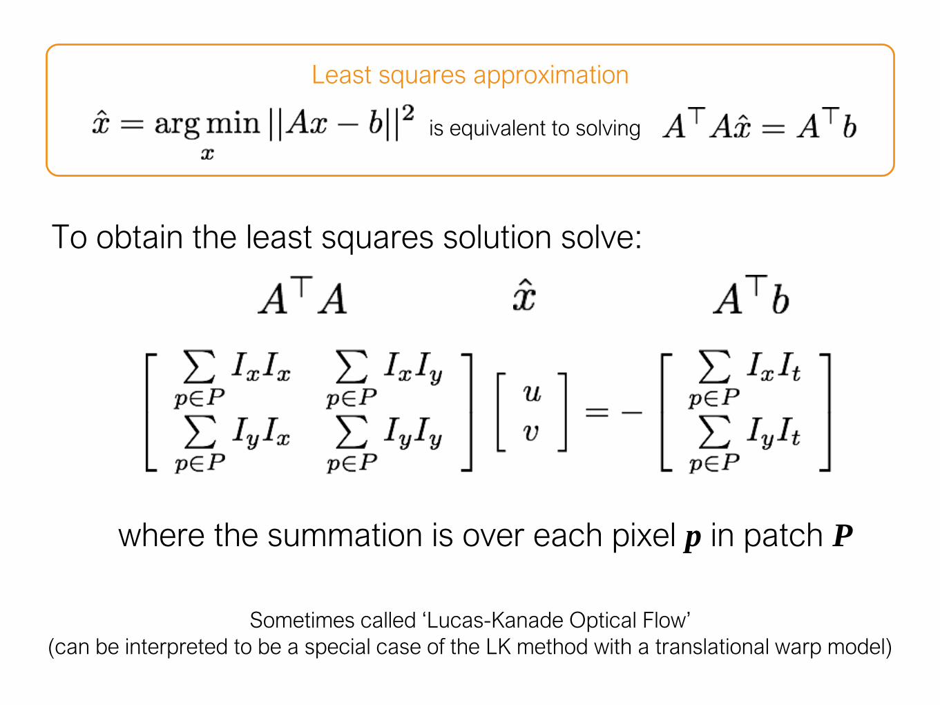
Least squares approximation
is equivalent to solving
where the summation is over each pixel p in patch P
Sometimes called ‘Lucas-Kanade Optical Flow’
(can be interpreted to be a special case of the LK method with a translational warp model)
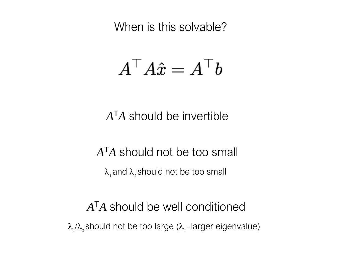
When is this solvable?
ATA should be invertible
ATA should not be too small
ATA should be well conditioned
l1and l
2should not be too small
l1/l
2should not be too large (l
1=larger eigenvalue)
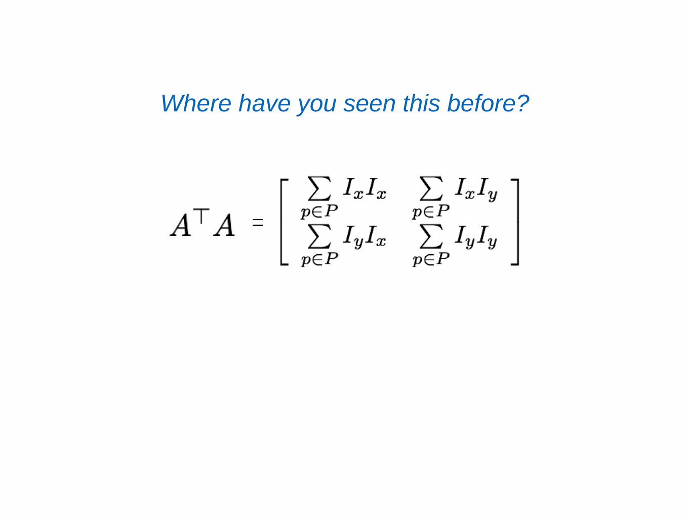
Where have you seen this before?
=
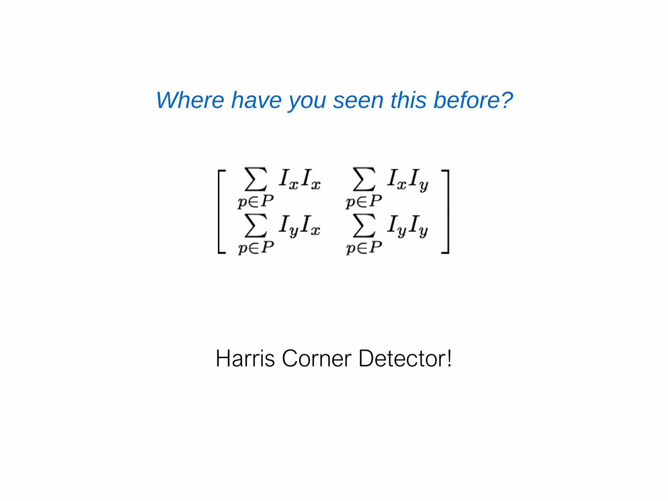
Where have you seen this before?
Harris Corner Detector!
Implications
• Corners are when λ1, λ2 are big; this is also when
Lucas-Kanade optical flow works best
• Corners are regions with two different directions of
gradient (at least)
• Corners are good places to compute flow!
What happens when you have no ‘corners’?
You want to compute optical flow.
What happens if the image patch contains only a line?

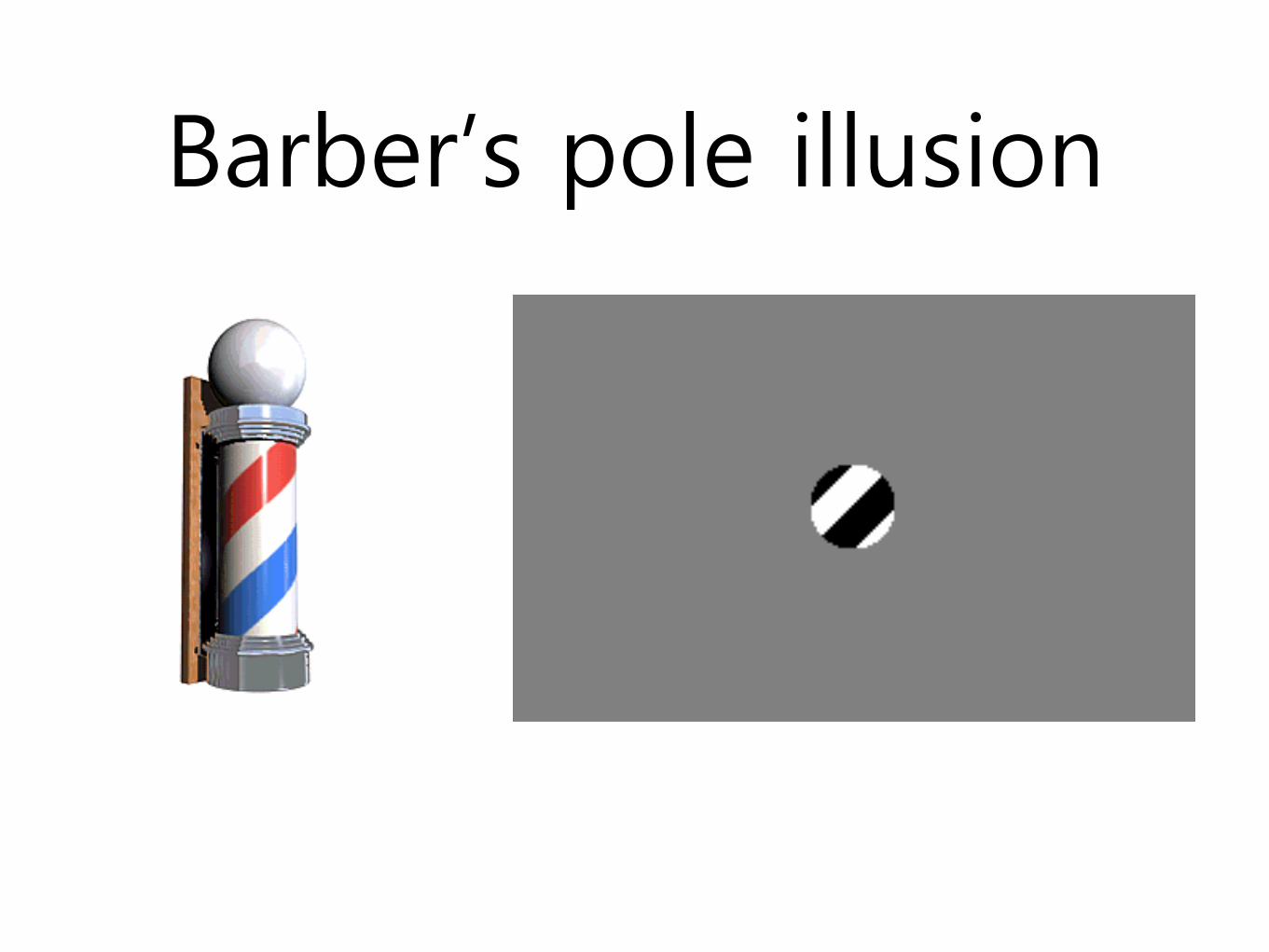
Barber’s pole illusion
Barber’s pole illusion
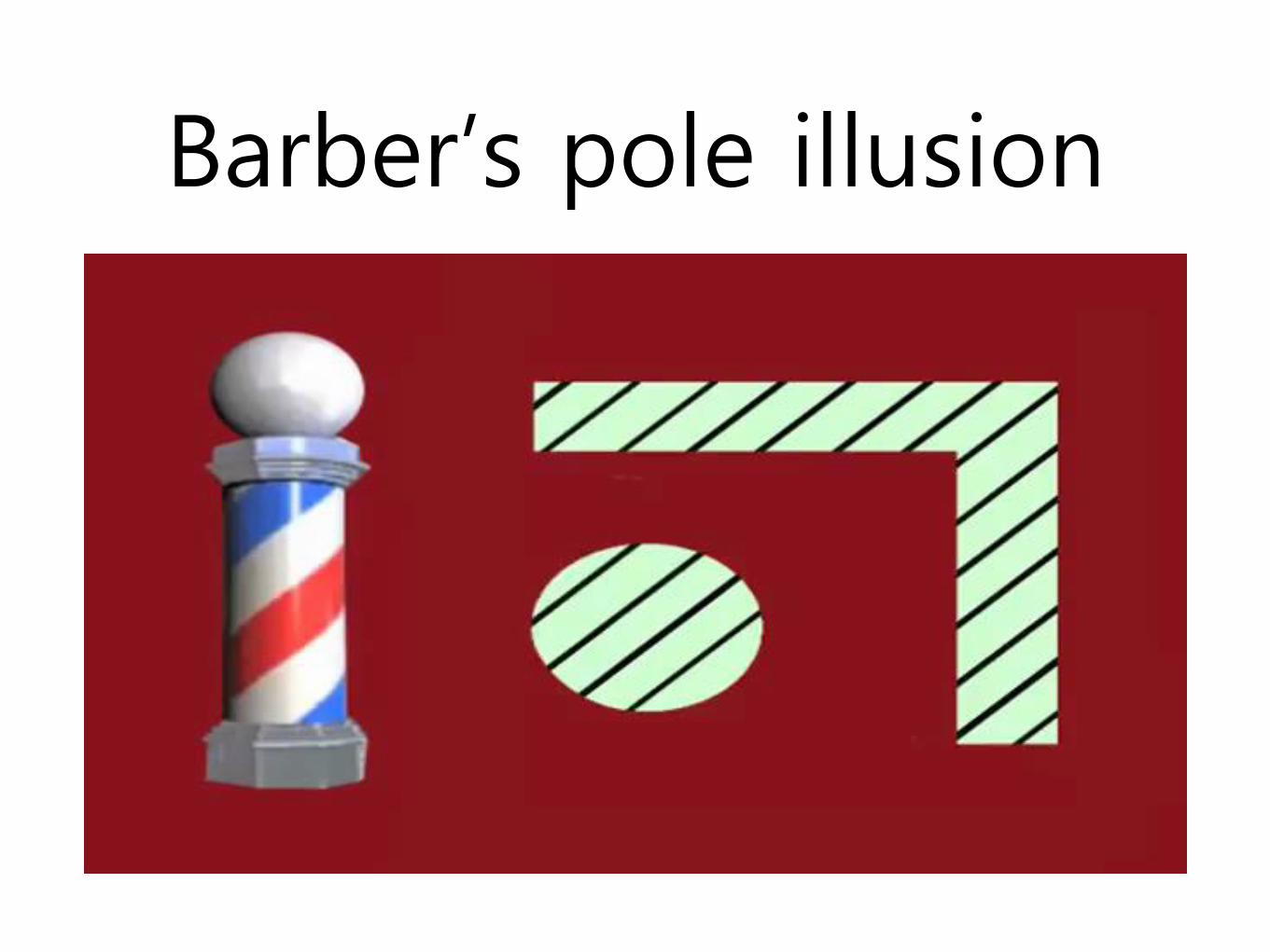
Barber’s pole illusion
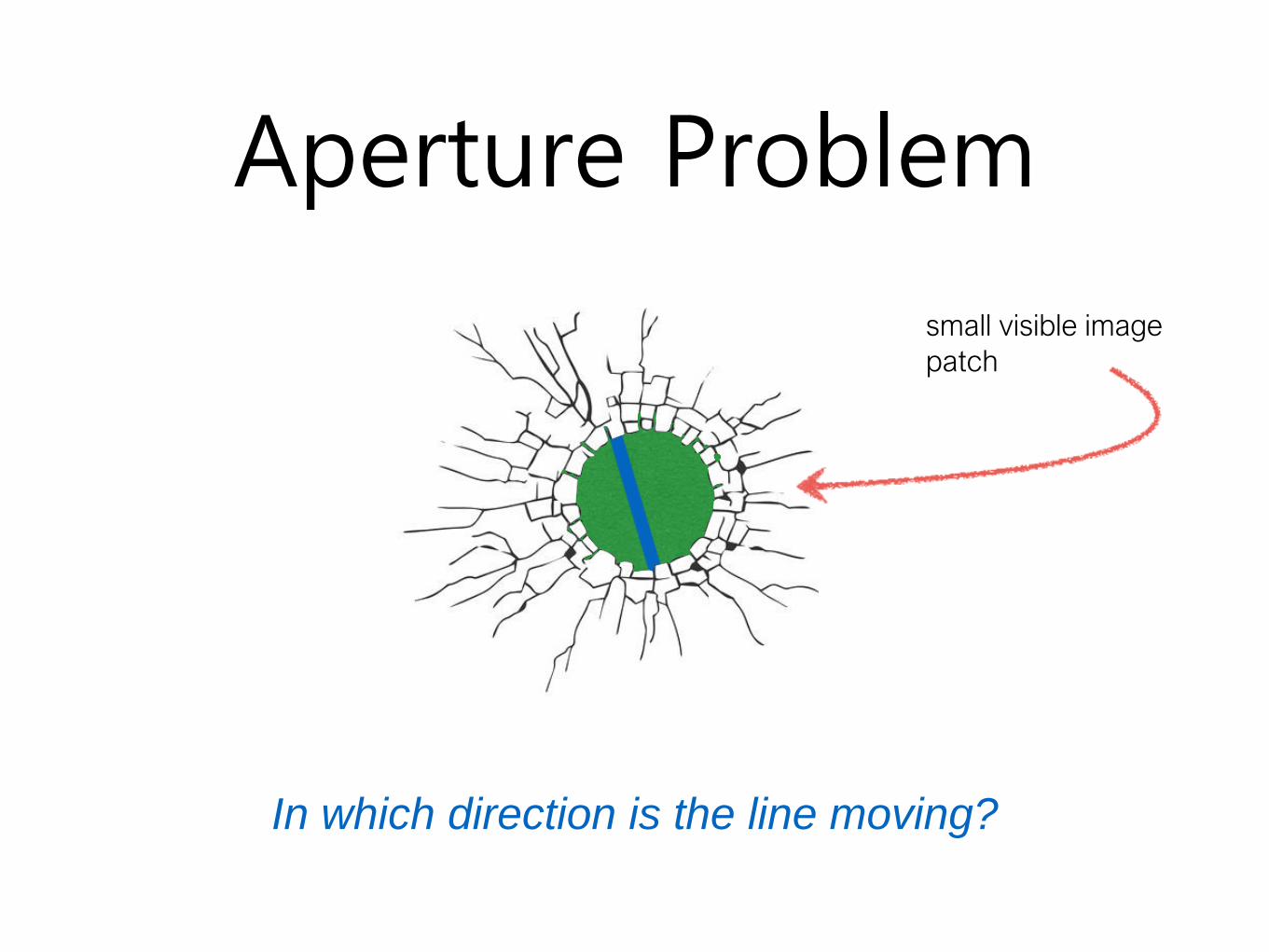
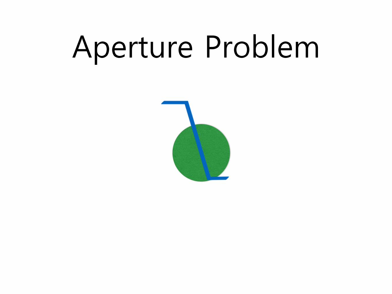
Aperture Problem
In which direction is the line moving?
small visible image
patch
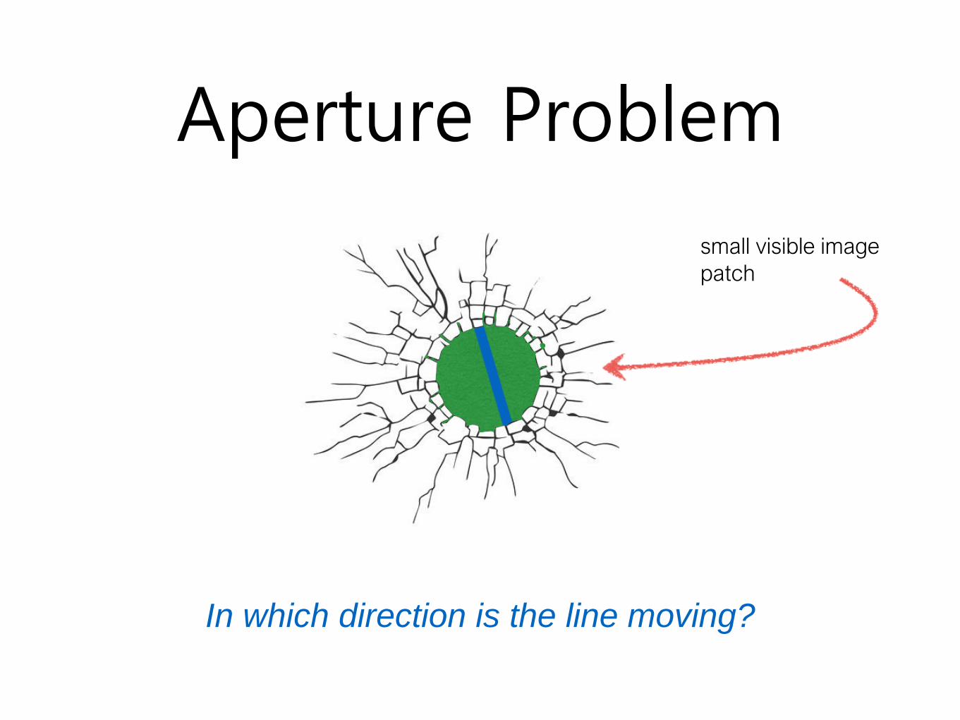
Aperture Problem
In which direction is the line moving?
small visible image
patch
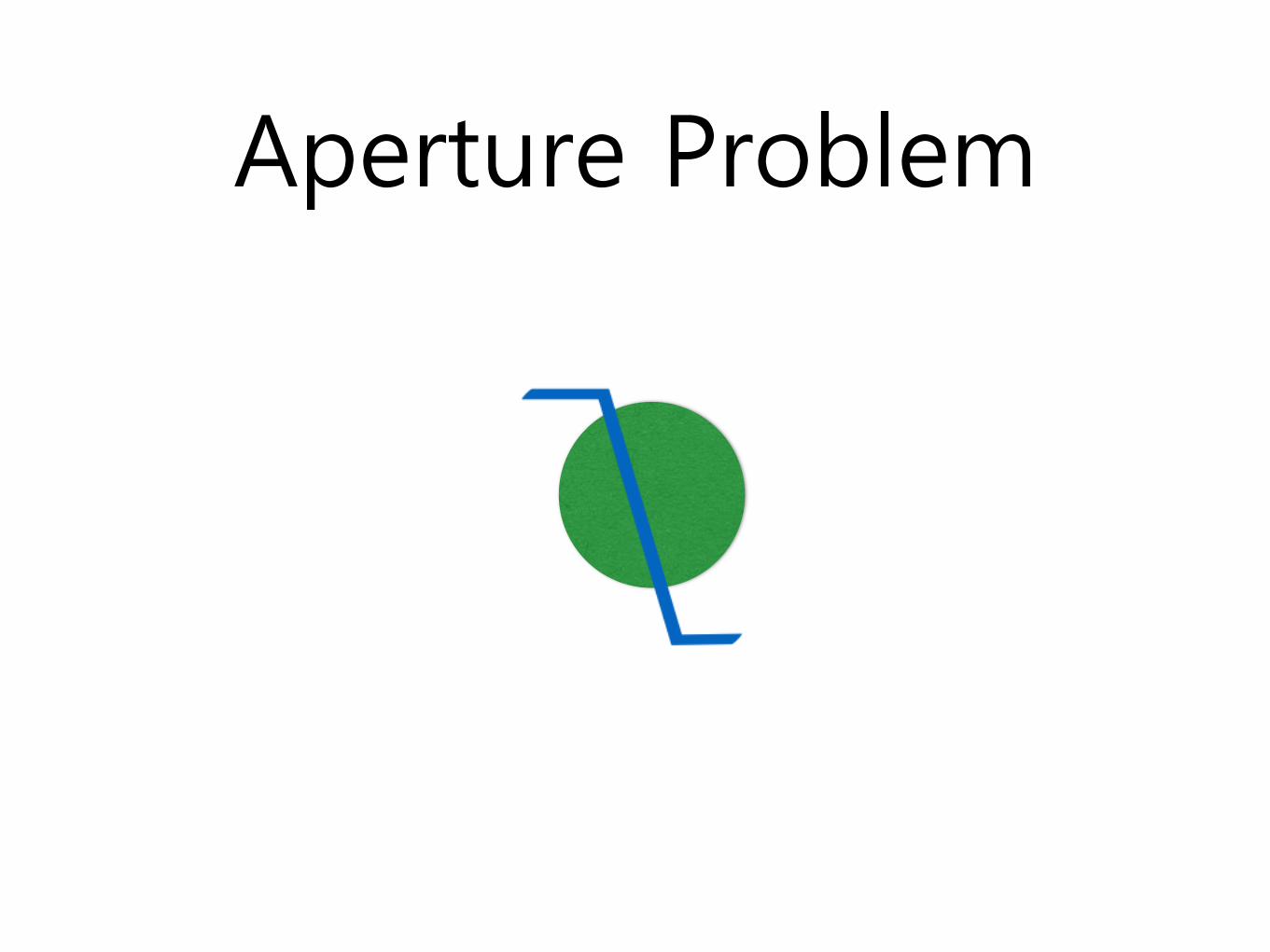
Aperture Problem
Aperture Problem

Aperture Problem
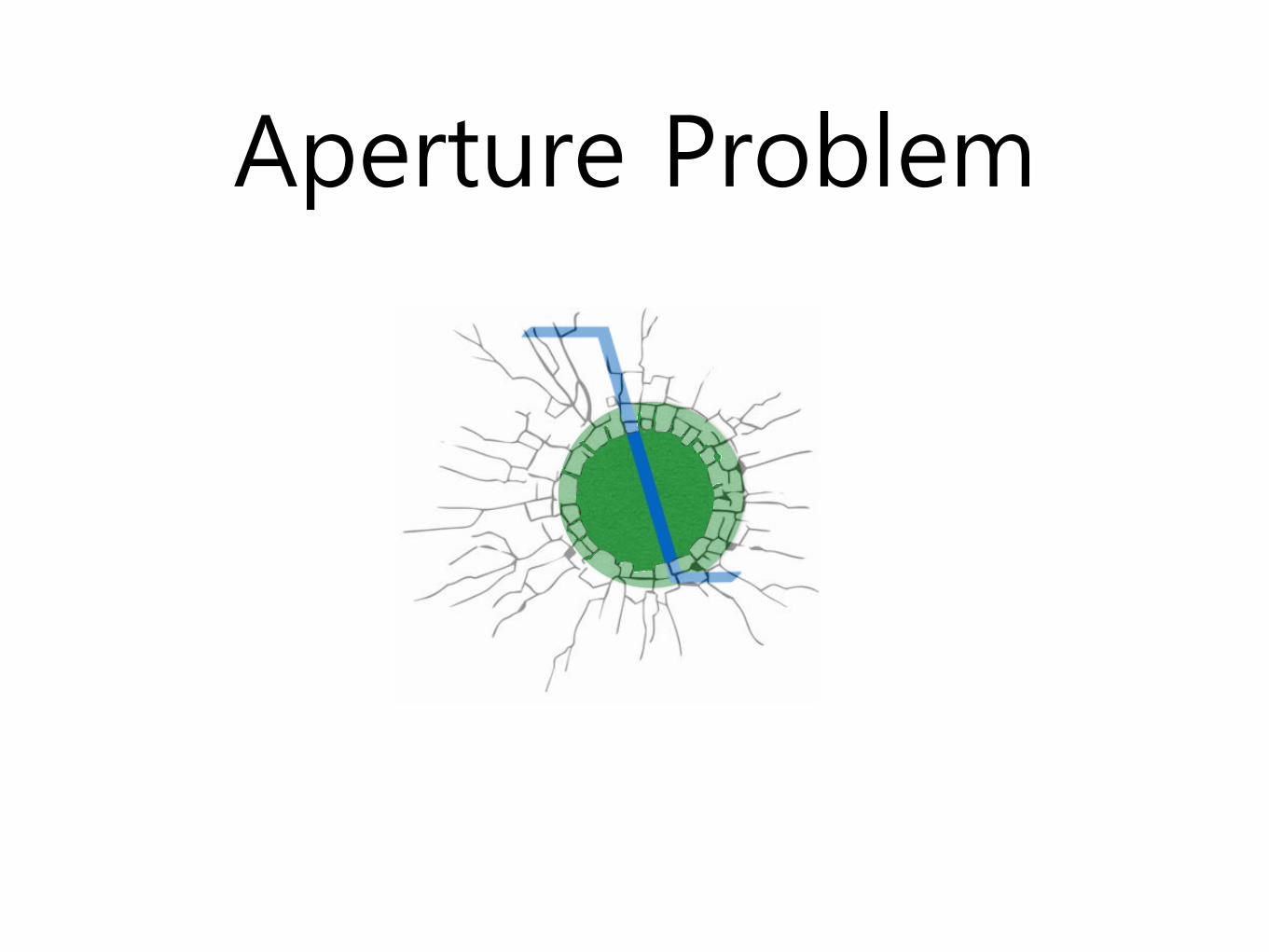
Aperture Problem
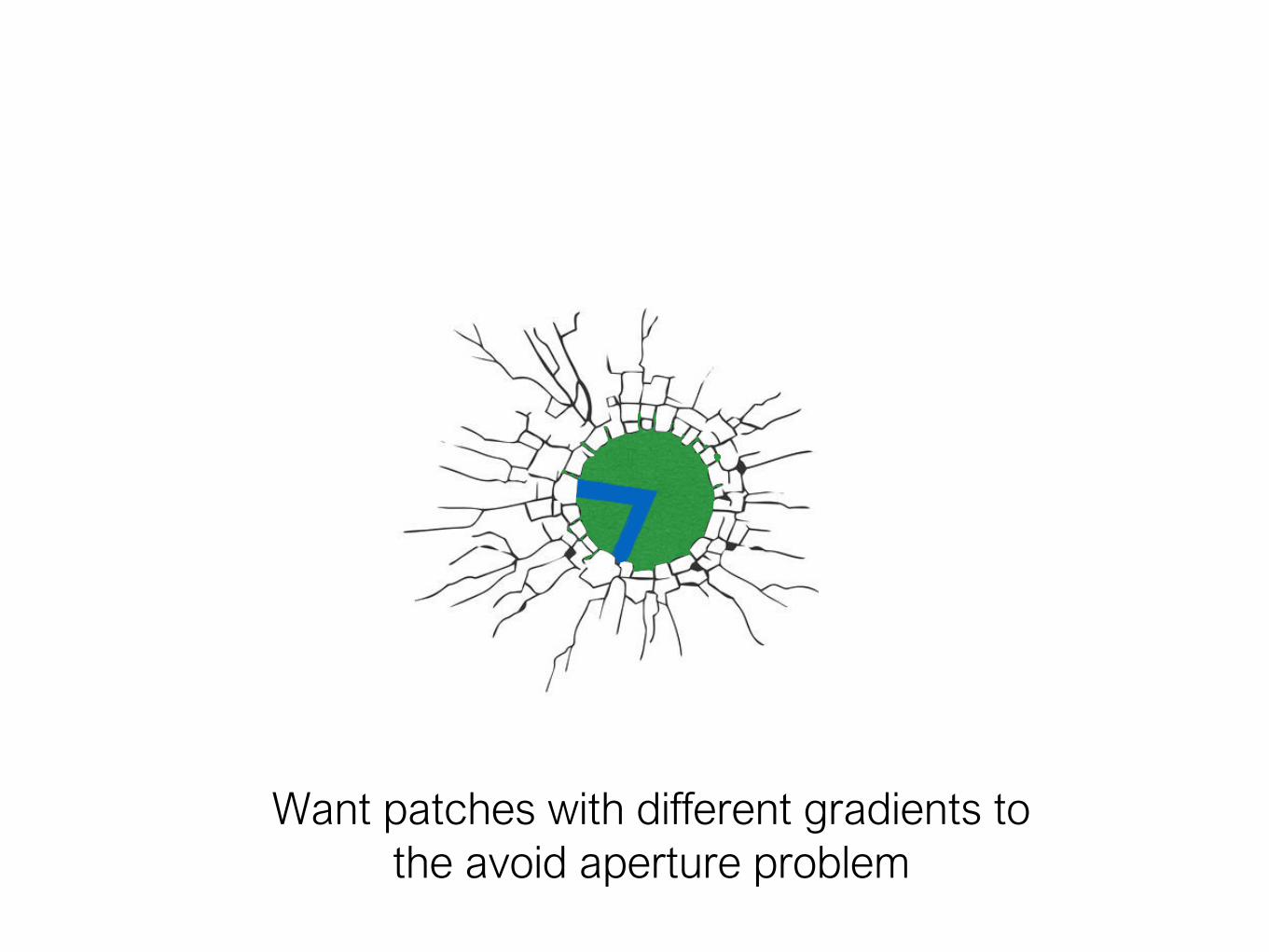
Want patches with different gradients to
the avoid aperture problem

Want patches with different gradients to
the avoid aperture problem
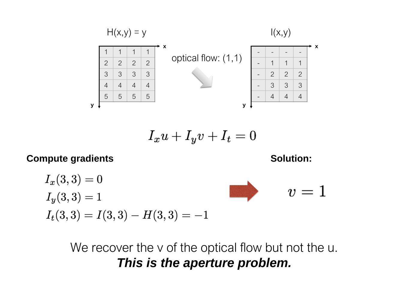
1 1 1 1
2 2 2 2
3 3 3 3
4 4 4 4
5 5 5 5
- - - -
- 1 1 1
- 2 2 2
- 3 3 3
- 4 4 4
y
x
y
x
optical flow: (1,1)
H(x,y) = y I(x,y)
We recover the v of the optical flow but not the u.
This is the aperture problem.
Compute gradients Solution:

Horn-Schunck optical flow
Horn-Schunck
Optical Flow (1981)
Lucas-Kanade
Optical Flow (1981)
‘constant’ flow(flow is constant for all pixels)
‘smooth’ flow(flow can vary from pixel to pixel)
brightness constancymethod of differences
global method
(dense)
local method
(sparse)
small motion

Smoothness
most objects in the world are rigid or
deform elastically
moving together coherently
we expect optical flow fields to be smooth
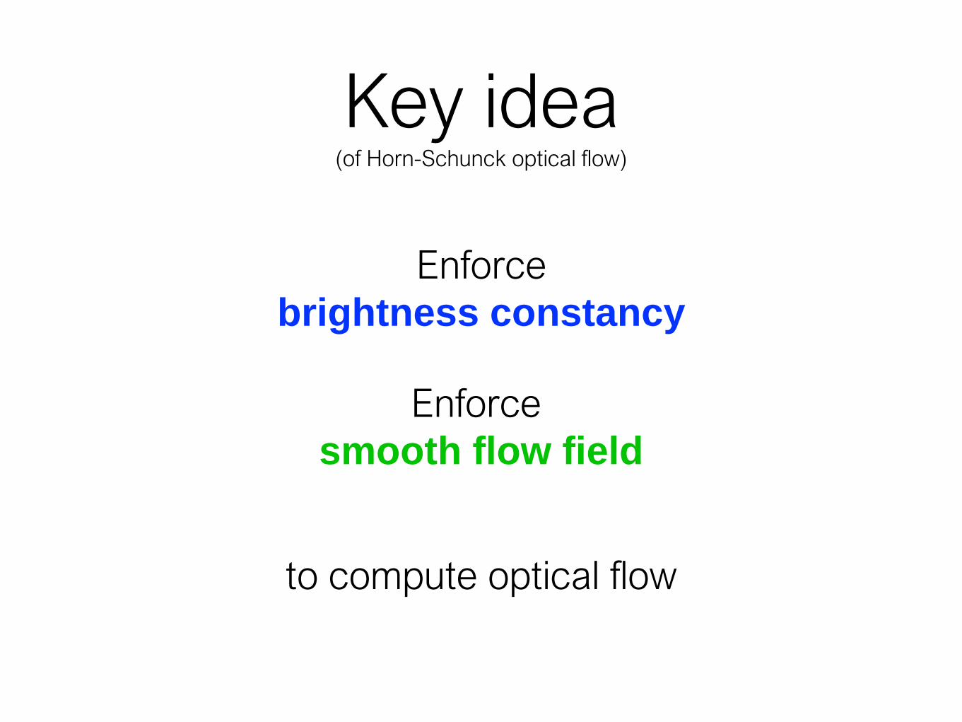
Key idea(of Horn-Schunck optical flow)
Enforce
brightness constancy
Enforce
smooth flow field
to compute optical flow

Key idea(of Horn-Schunck optical flow)
Enforce
brightness constancy
Enforce
smooth flow field
to compute optical flow
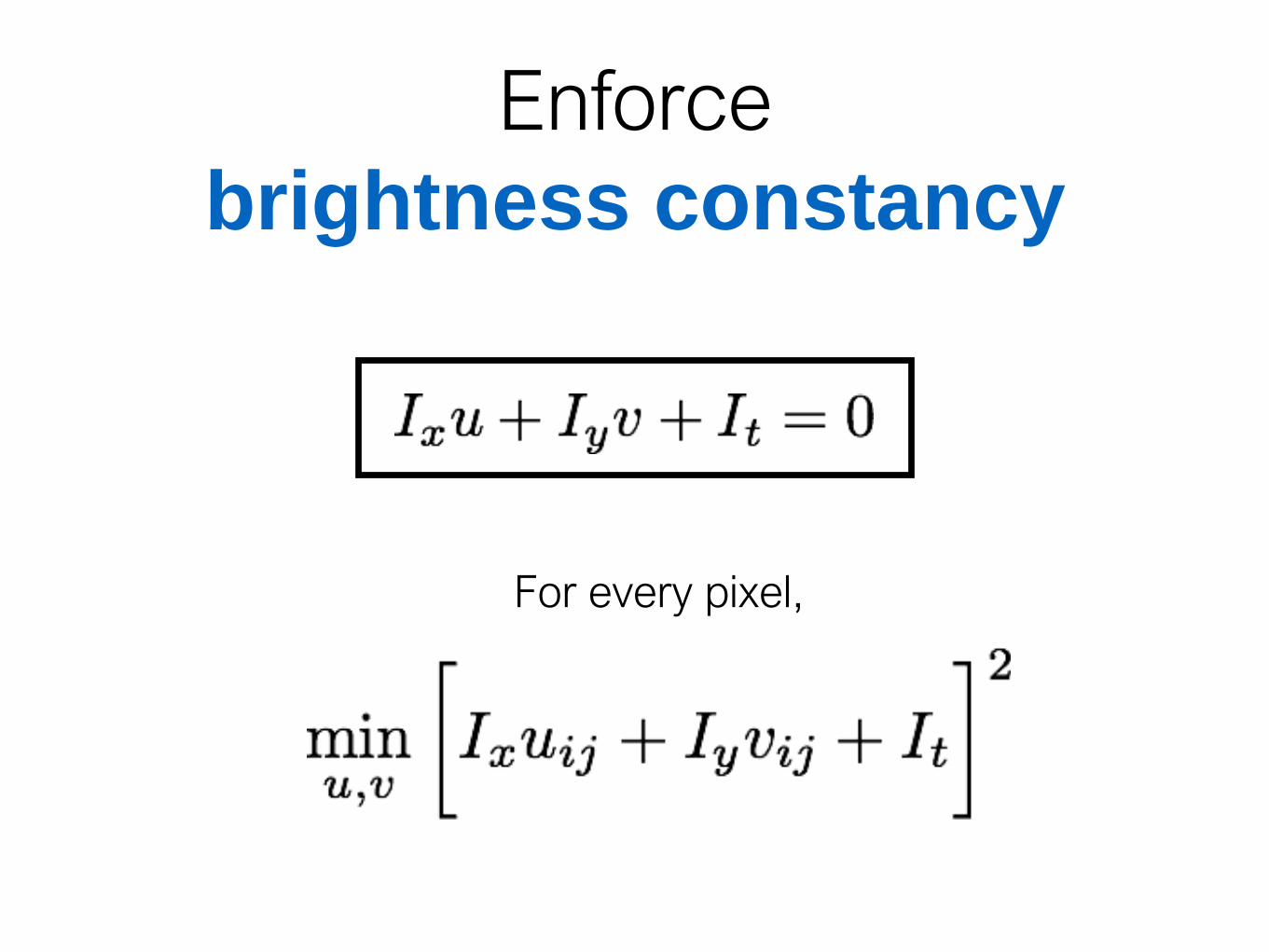
Enforce
brightness constancy
For every pixel,

For every pixel,
lazy notation for
Enforce
brightness constancy
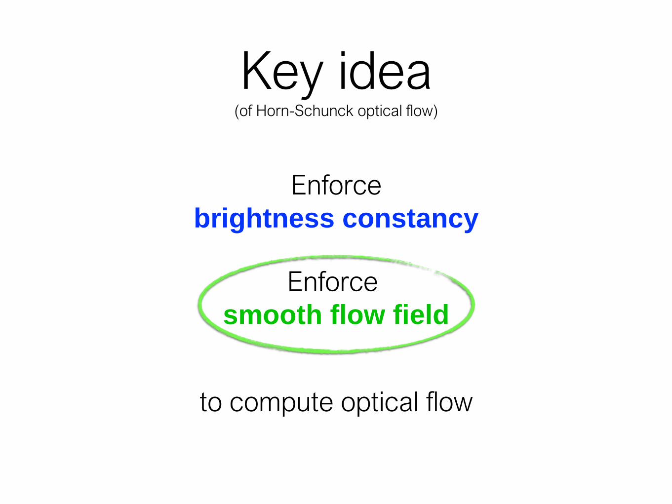
Key idea(of Horn-Schunck optical flow)
Enforce
brightness constancy
Enforce
smooth flow field
to compute optical flow

Enforce smooth flow field
u-component of flow
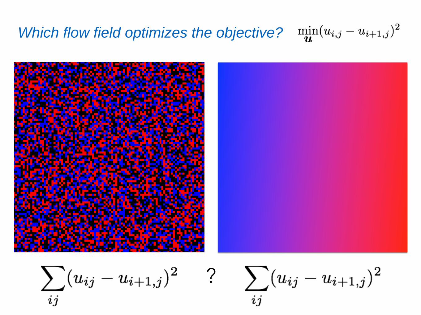
Which flow field optimizes the objective?
?
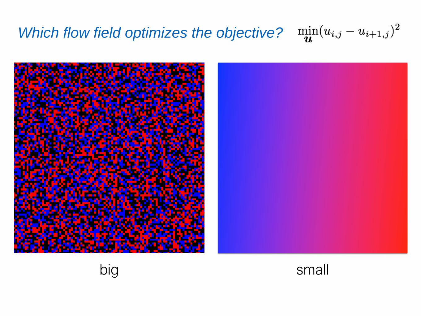
smallbig
Which flow field optimizes the objective?

Key idea(of Horn-Schunck optical flow)
Enforce
brightness constancy
Enforce
smooth flow field
to compute optical flow
bringing it all together…

Horn-Schunck optical flow
smoothness brightness constancy
weight

HS optical flow objective function
Brightness constancy
Smoothness
why not all four neighbors?

How do we solve this
minimization problem?

Compute partial derivative, derive update equations(gradient decent!)
How do we solve this
minimization problem?
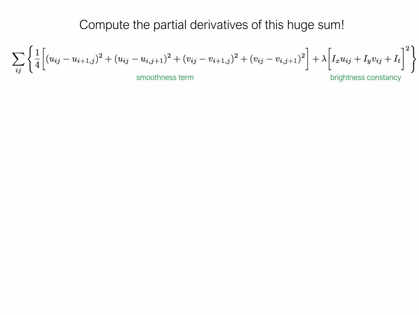
Compute the partial derivatives of this huge sum!
smoothness term brightness constancy
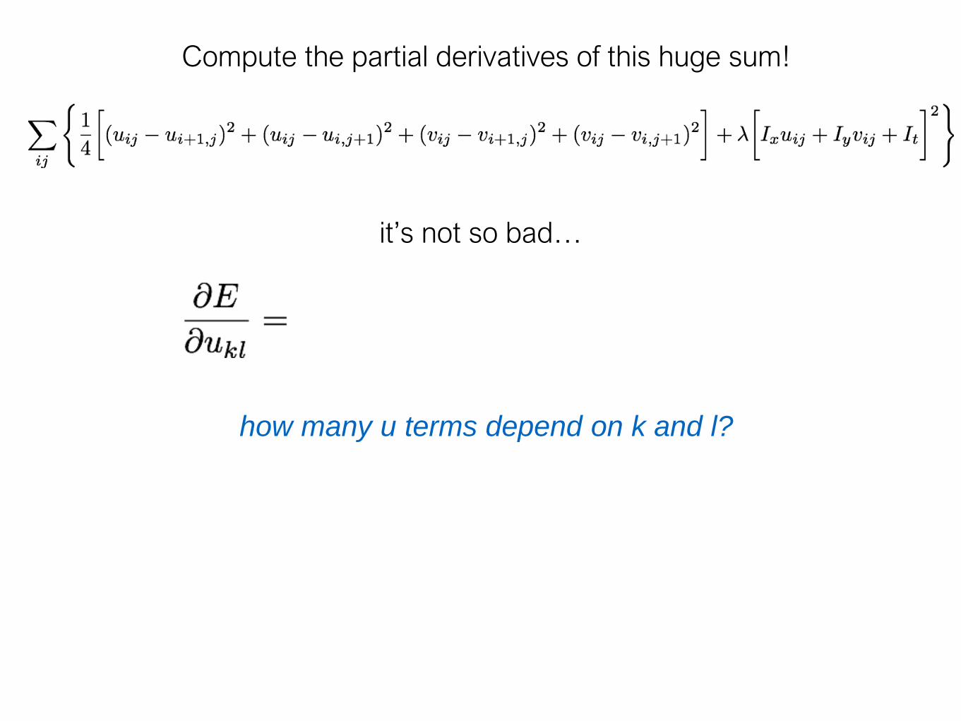
Compute the partial derivatives of this huge sum!
it’s not so bad…
how many u terms depend on k and l?

Compute the partial derivatives of this huge sum!
it’s not so bad…
how many u terms depend on k and l?
ONE from brightness constancyFOUR from smoothness

Compute the partial derivatives of this huge sum!
it’s not so bad…
how many u terms depend on k and l?
ONE from brightness constancyFOUR from smoothness

Compute the partial derivatives of this huge sum!
(variable will appear four times in sum)

Compute the partial derivatives of this huge sum!
short hand for
local average
(variable will appear four times in sum)
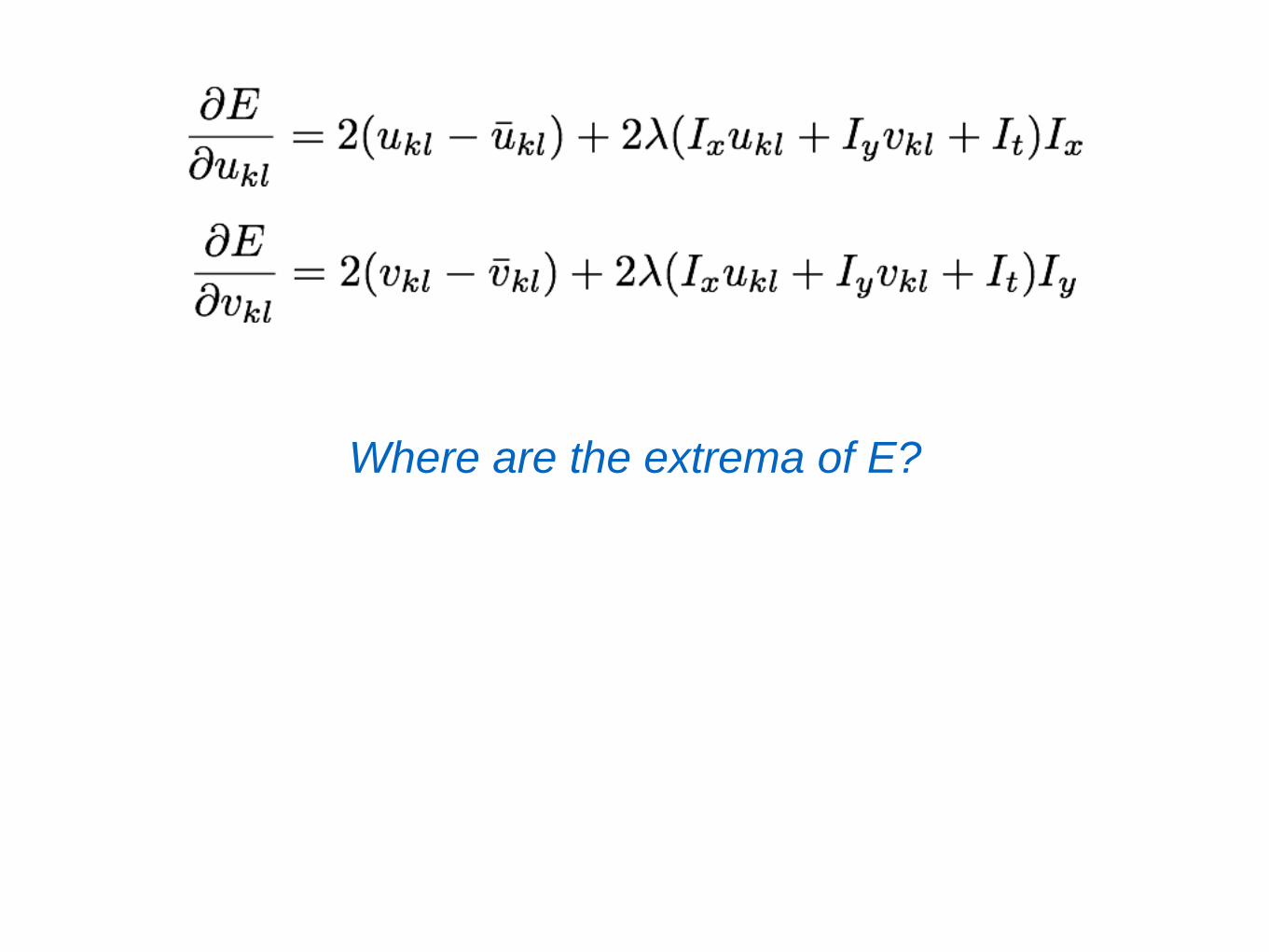
Where are the extrema of E?

Where are the extrema of E?
(set derivatives to zero and solve for unknowns u and v)

Where are the extrema of E?
(set derivatives to zero and solve for unknowns u and v)
how do you solve this?this is a linear system

ok, take a step back, why are we doing all this math?

We are solving for the optical flow (u,v) given two
constraints
smoothness brightness constancy
We need the math to minimize this
(back to the math)

Where are the extrema of E?
(set derivatives to zero and solve for unknowns u and v)
how do you solve this?
Partial derivatives of Horn-Schunck objective function E:

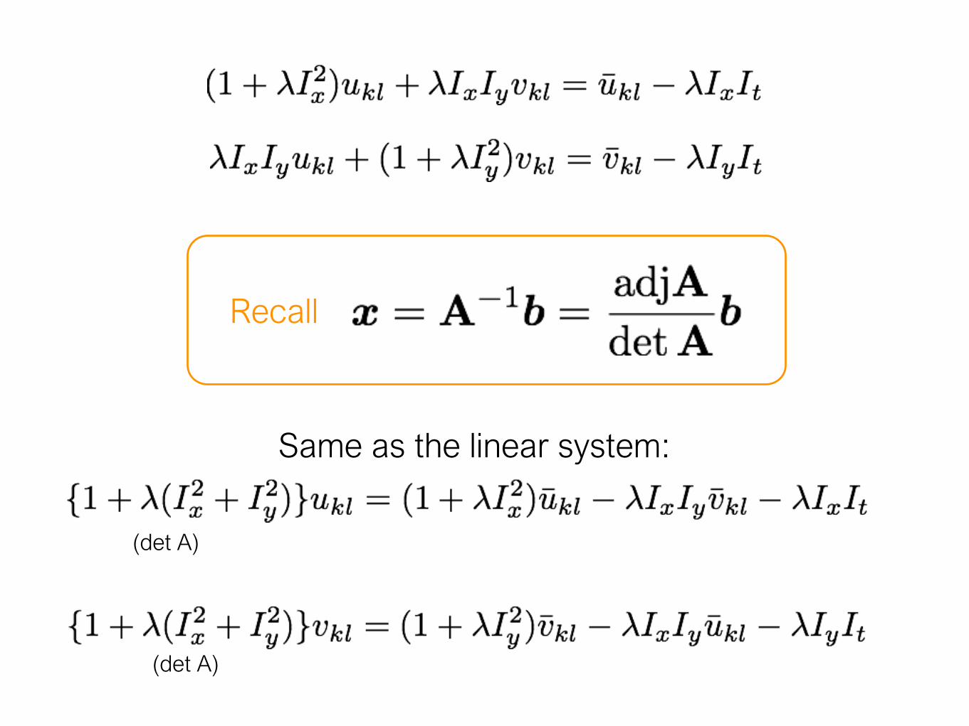
Recall
Recall
(det A)
Same as the linear system:
(det A)
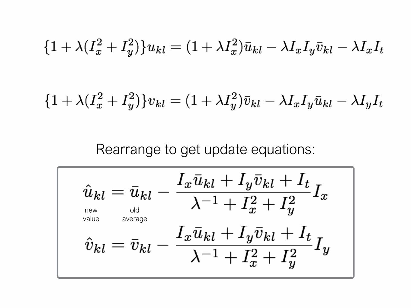
Rearrange to get update equations:
new
value
old
average

new
value
old
average
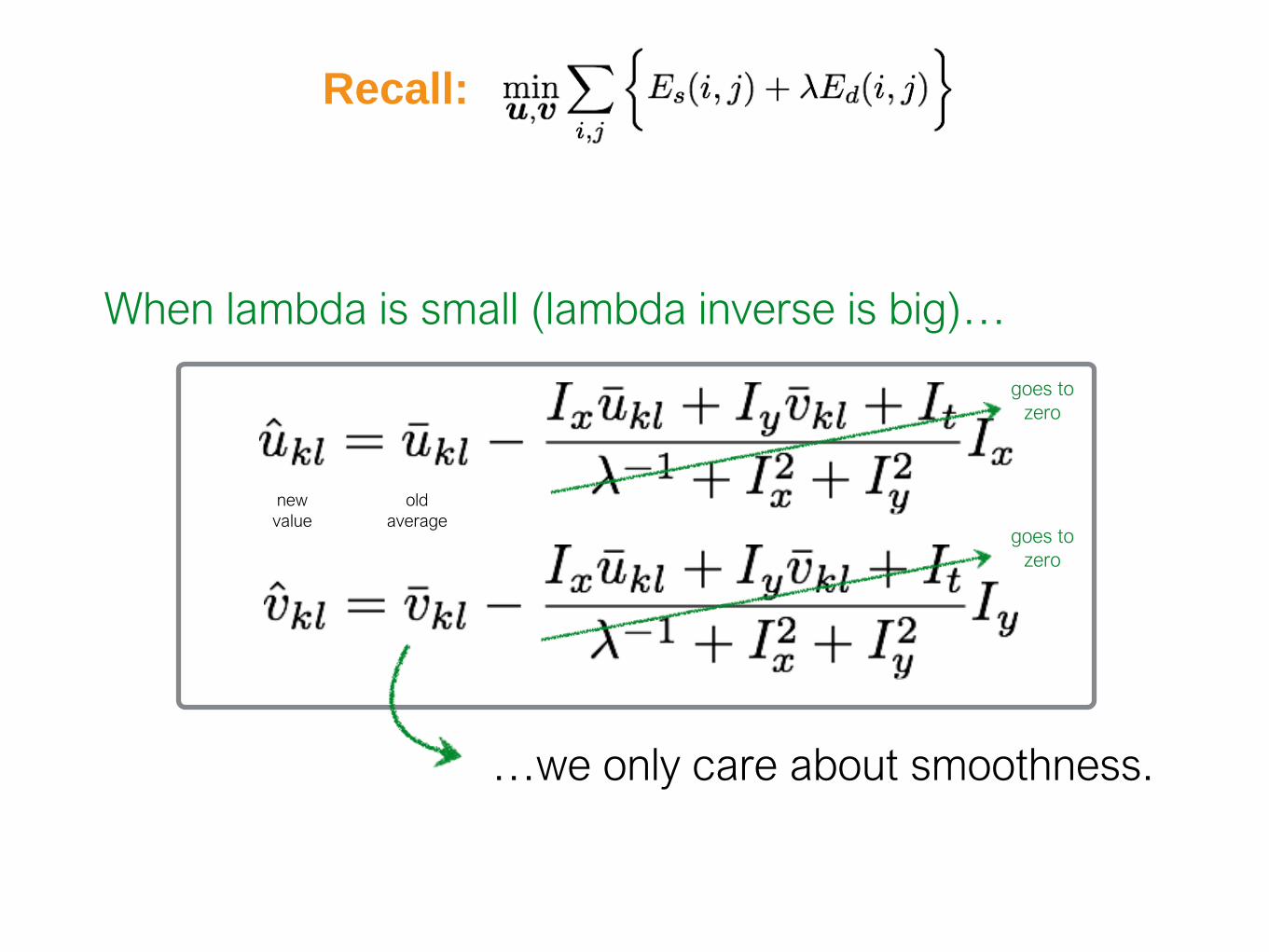
When lambda is small (lambda inverse is big)…
Recall:

new
value
old
average
When lambda is small (lambda inverse is big)…
goes to
zero
goes to
zero
Recall:
new
value
old
average
When lambda is small (lambda inverse is big)…
goes to
zero
goes to
zero
…we only care about smoothness.
Recall:

ok, take a step back, why did we do all this math?

We are solving for the optical flow (u,v) given two
constraints
smoothness brightness constancy
We needed the math to minimize this
(now to the algorithm)

Horn-Schunck
Optical Flow Algorithm
1. Precompute image gradients
2. Precompute temporal gradients
3. Initialize flow field
4. While not converged
Compute flow field updates for each pixel:
Just 8 lines of code!

References
Basic reading:• Szeliski, Section 8.4.