Optical fiber power meter nonlinearity calibrations at NIST · Government. As anagency of theU.S. Commerce Department'sTechnologyAdministration, NISTconducts basic and appliedresearch

NAT'L INST. OF STAND & TECH

msTPUBUCATiONS

NIST Measurement Services:

Optical Fiber Power IVIeter

Nonlinearity Calibrations at NIST

NISTSpecial

Publication

250-56

Igor VayshenkerShao YangXiaoyu Li

Thomas R. Scott

Christopher L. Cromer

C00

57

1.250-56

1)00

NIST CENTENNIAL

iisr National institute of Standards and Technology • Technology Administration • U.S. Department of Commerce

M he National Institute of Standards and Teclinology was established in 1988 by Congress to "assist industry in

the development of technology . . . needed to improve product quality, to modernize manufacturing processes, to

ensure product reliability ... and to facilitate rapid commercialization ... of products based on new scientific

discoveries."

NIST, originally founded as the National Bureau of Standards in 1901, works to strengthen U.S. industry's

competitiveness; advance science and engineering; and improve public health, safety, and the environment. Oneof the agency's basic functions is to develop, maintain, and retain custody of the national standards of

measurement, and provide the means and methods for comparing standards used in science, engineering,

manufacturing, commerce, industry, and education with the standards adopted or recognized by the Federal

Government.

As an agency of the U.S. Commerce Department's Technology Administration, NIST conducts basic and

applied research in the physical sciences and engineering, and develops measurement techniques, test

methods, standards, and related services. The Institute does generic and precompetitive work on new and

advanced technologies. NIST's research facilities are located at Gaithersburg, MD 20899, and at Boulder, CO 80303.

Major technical operating units and their principal activities are listed below. For more information contact the

Publications and Program Inquiries Desk, 301-975-3058.

Office of the Director• National Quality Program

• international and Academic Affairs

Technology Services• standards Services

• Technology Partnerships

• Measurement Services

• Information Services

Advanced Technology Program• Economic Assessment• Information Technology and Applications

• Chemistry and Life Sciences

• Materials and Manufacturing Technology

• Electronics and Photonics Technology

Manufacturing Extension PartnershipProgram• Regional Programs• National Programs• Program Development

Electronics and Electrical EngineeringLaboratory• Microelectronics

• Law Enforcement Standards

• Electricity

• Semiconductor Electronics

• Radio-Frequency Technology^

• Electromagnetic Technology^

• Optoelectronics^

Materials Science and EngineeringLaboratory• Intelligent Processing of Materials

• Ceramics

• Materials Reliability^

• Polymers

• Metallurgy

• NIST Center for Neutron Research

Chemical Science and TechnologyLaboratory• Biotechnology

• Physical and Chemical Properties^

• Analytical Chemistry

• Process Measurements• Surface and Microanalysis Science

Physics Laboratory• Electron and Optical Physics

• Atomic Physics

• Optical Technology

• Ionizing Radiation

• Time and Frequency^

• Quantum Physics^

Manufacturing EngineeringLaboratory• Precision Engineering

• Automated Production Technology

• Intelligent Systems• Fabrication Technology

• Manufacturing Systems Integration

Building and Fire ResearchLaboratory• Applied Economics• Structures

• Building Materials

• Building Environment

• Fire Safety Engineering

• Fire Science

Information Technology Laboratory• Mathematical and Computational Sciences^

• Advanced Network Technologies

• Computer Security

• Information Access and User Interfaces

• High Performance Systems and Services

• Distributed Computing and Information Services

• Software Diagnostics and Conformance Testing

• Statistical Engineering

'At Boulder, CO 80303.

^Some elements at Boulder, CO.

Errata Sheet for NIST Special Publication 250-56 (August2000)

The word "Nonlinearity" was omitted from the title on thedocument title page (page i).

Please tape the attached corrected title page over theincorrectly printed one.

Note that the correction is for page i only and does notinclude the bibliographic data that appears on the printed"verso" (page ii)

.

NIST Special Publication 250-56

NIST MEASUREMENT SERVICES:Optical Fiber Power MeterNonlinearity Calibrations at NIST

Igor Vayshenker

Shao Yang*

Xiaoyu Li

Thomas R. Scott


Optoelectronics Division

Electronics and Electrical Engineering Laboratory

National Institute of Standards and Technology

Boulder, CO 80305-3328

*Biostar

6655 Lookout RoadBoulder, CO 80301

August 2000

U.S. Department of CommerceNorman Y. Mineta, Secretary

Technology Administration

Dr Cheryl L. Shavers, Under Secretary of Commerce for Technology


Raymond G. Kammer, Director

/

V

NIST Special Publication 250-56

NIST MEASUREMENT SERVICES:Optical Fiber Power IVleter Calibrations at NIST

Igor Vayshenker

Shao Yang*

Xiaoyu Li

Thomas R. Scott



Electronics and Electrical Engineering Laboratory


Boulder, CO 80303

*Biostar

6655 Lookout RoadBoulder, CO 80301

August 2000

U.S. Department of CommerceNorman Y. Mineta, Secretary

Technology Administration

Dr. Cheryl L. Stiavers, Under Secretary of Commerce for Technology


Raymond G. Kammer, Director

Certain commercial entities, equipment, or materials may be identified in this document in order to

describe an experimental procedure or concept adequately. Such identification is not intended to imply

recommendation or endorsement by the National Institute of Standards and Technology, nor is it intended

to imply that the entities, materials, or equipment are necessarily the best available for the purpose.

National Institute of Standards and Technology Special Publication 250-56

Natl. Inst. Stand. Technol. Spec. Publ. 250-56, 34 pages (August 2000)

CODEN: NSPUE2

U.S. GOVERNMENT PRINTING OFFICEWASHINGTON: 2000

For sale by the Superintendent of Documents, U.S. Government Printing Office, Washington, DC 20402-9325

Contents

1. Introduction 1

2. Measurement ofNonlinearity and Range Discontinuity 1

2. 1 Definition and Basic Expressions 2

2.2 Polynomial Expression for Conversion Function 4

2.2.1 Triplet Superposition Method 5

2.3 Correction Factor for Nonlinearity and Range Discontinuity 6

3. Nonlinearity Measurement System 8

4. Uncertainty Assessment 11

5. References 17

Appendix A. Laser Diode Optical Spectra 18

Appendix B. Measurement Flow Chart 19

Appendix C. Sample of a Calibration Report 20

iii

Optical Fiber Power Meter Nonlinearity Calibrations at NIST

Igor Vayshenker, Shao Yang*, Xiaoyu Li, Thomas R. Scott, and Christopher L. Cromer

National Institute of Standards and Technology, 325 Broadway, Boulder, CO 80303

*Biostar, 6655 Lookout Rd, Boulder, CO 80301

We describe a system for measuring the response nonlinearity of optical fiber

power meters and detectors over a wide power dynamic range at

telecommunication wavelengths. The system uses optical fiber components and is

designed to accommodate commonly used optical fiber power meters. The system

also measures the range discontinuities between neighboring power ranges or scale

settings of the optical fiber power meter. Measurements with this system yield

correction factors for all power ranges ofthe meter. The measurement system is

capable of producing results which have standard deviations as low as 0.01 %.

The measurement uncertainties associated with the system are described.

Key words: calibration; detector; linearity; measurement service; nonlinearity;

optical fiber power meter; optical power; range discontinuity; uncertainty.

1. Introduction

There are several methods currently used for the measurement of optical fiber power meter

(OFPM) or detector nonlinearity: differential, attenuation, and superposition. These methods

were compared analytically using a unified mathematical expression for nonlinearity [1-3]. Based

on these results, we developed a system, which uses a superposition method known as the triplet

method. This method relies on the principle that for a linear OFPM, the sum of the OFPMoutputs corresponding to inputs fi"om two individual beams should equal the output when the two

beams are combined and incident on the OFPM at the same time. The triplet method does not

require a standard; a measurement system based on the triplet method is the standard by itself

2. Measurement of Nonlinearity and Range Discontinuity

Generally, an OFPM has a dynamic range of more than 60 dB with many meters exceeding 90 dB.

To achieve these dynamic ranges, an OFPM is designed to switch ranges during optical power

measurements. The power ranges have their own gains or amplifications, which ofl;en differ by a

factor of 10. When the meter switches fi"om one range to another, it is critical that two

neighboring ranges indicate the same power. If the power readings at these two ranges are not

the same, then the OFPM has a range discontinuity (assuming the power has remained constant).

A simplified schematic of a typical OFPM is depicted in Figure 1

.

1

DETECTOR

—m—lOOORf

—m—100 Rf

—m—FEEDBACKRESISTORRf

OPERATIONALAMPLIFIER

Figure 1 . Simplified schematic of a typical optical power meter.

The NIST nonlinearity system is capable of measuring the nonlinearity ofOFPMs over a dynamic

range of more than 60 dB at the three nominal telecommunication wavelengths: 850, 1300, and

1550 nm. This system uses optical fiber components and is designed to accommodate commonly

used OFPMs and other optical detectors. The system also measures the range discontinuity

between neighboring power ranges or scale settings of the OFPM. Measurements with this

system yield a correction factor for each power range of an OFPM. Note: for a bare detector, the

ranges may be the electrical voltage or current ranges of the output electronics.

2.1 Definition and Basic Expressions

The nonlinearity of an OFPM is defined as the relative difference between the responsivity at an

arbitrary power and the responsivity at the calibration power (i.e., the power at which the meter

was calibrated). This definition can be expressed as

R(P) - R(P^ )A,,(P;P ) =

^^^Î

- \ (1)

where R(P) = V/P is the responsivity of the OFPM at incident optical power P; the subscript c

indicates the calibration point, and V is the OFPM output, which can be electrical current.

2

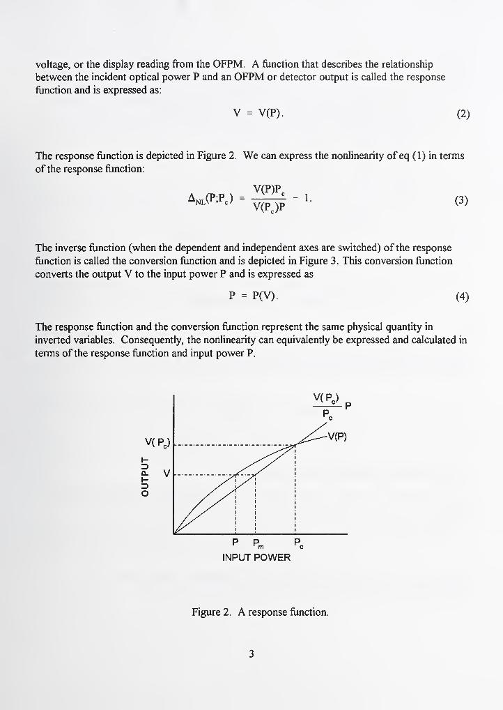
voltage, or the display reading from the OFPM. A function that describes the relationship

between the incident optical power P and an OFPM or detector output is called the response

function and is expressed as:

V = V(P). (2)

The response function is depicted in Figure 2. We can express the nonlinearity of eq (1) in terms

ofthe response function:

V(P)P,^N.(P;Pe) =^ - (3)

The inverse function (when the dependent and independent axes are switched) of the response

function is called the conversion function and is depicted in Figure 3. This conversion function

converts the output V to the input power P and is expressed as

P = P(V). (4)

The response function and the conversion function represent the same physical quantity in

inverted variables. Consequently, the nonlinearity can equivalently be expressed and calculated in

terms of the response function and input power P.

' m c

INPUT POWER

Figure 2. A response function.

3

V Vc

OUTPUT

Figures. A conversion function.

In practice, it is often more convenient to use the conversion function rather than the response

function. We can define the nonlinearity in terms of the output V as

P(V, )VV(v;v. ) = - 1. (5)

2.2 Polynomial Expression for Conversion Function

When the nonlinearity is small, a polynomial can represent the conversion function well [4,5];

that is

P(V) = Ea,V\ (6)k=l

where n is the order ofthe polynomial and a^^ are the coefficients of the polynomial. The

coefficients a^ correspond to a calibrated conversion function [1].

4

The output responses of the commonly used photodiodes, Si, Ge, or InGaAs, are exponential (see

conversion function in Figure 3) with respect to the input power. However, they are often used in

nearly short-circuited or reverse-biased configurations to achieve a linear response. As a result,

their responses can be approximated as polynomials produced by the Taylor-series expansion of

the form shown in eq (6), where the zero-order term is not included because we always measure

the dark signal and later subtract it fiôm the output of an OFPM. With the assumption of

f^^ V^-^ « 1,

k=2 aj

the nonlinearity A^l of eq (5) can be approximated by (for the nonlinearity of less than 1 %, the

approximation error is less than 0.01 %)

V(v;v,) ^ -E -(V^-^ - v^'). (7)k=2 aj

Ifwe divide all the coefficients a^ in eq (6) by the first coefficient aj, the polynomial thus obtained

is called the normalized conversion function, denoted by p(V) and expressed as

p(V) = V ^ E ^ (8)k=2

where b^ = a^/aj. The coefficients b^ correspond to an uncalibrated conversion function described

in reference [1]. Typically, n is equal to 3.

The nonlinearity can be expressed as

V(V;V,) - -twc^""' - v^'). (9)k=2

2.2.1 Triplet Superposition Method

In the triplet superposition method, a group of three power measurements is made, two for

individual powers from each beam and one for the combination of the two. For the i* group of

measurements, we have a set of three equations:

5

Pli= Vh - Eb.Vit,

k=2

P2i= . t^V^-, (10)

k=2

n

Pli P2i = + E^k^Si,k=2

where the p; are arbitrary unknowns and the V; are measured output values. A new equation

is formed by subtracting the first and second equations fiôm the tliird equation while eliminating

the unknown pj in the group ofthe three equations in eq (10):

(V3i - - V,;) EW- - V,^ - V^^) = 0. (11)k=2

The coefficients b^ can be obtained by linear least-squares fitting of the measured data. The three

measurement runs are usually made in immediate succession, which helps reduce the uncertainty

that might occur due to drift of the laser source output. The details of the measurements are

described in Section 3.

2.3 Correction Factor for Nonlinearity and Range Discontinuity

While calibration gives the true relationship between the input power and the OFPM reading

(output) at the calibration point, the measurement of nonlinearity and range discontinuity,

together with calibration, provides this input-output relation at any power over the whole dynamic

range of the OFPM. It is, therefore, convenient to express the measured nonlinearity, A-^^Vyjin terms of the conversion fiinction P = P(V), which relates the input power P to the output V,

referred to the calibration output V^..

We denote the range setting of the OFPM with brackets; [m] denotes some range m (m = 1, 2,

3,...), and [c] is the range where the reference power is used. Calibration determines in range

[c] where the calibration reference point is selected; P^ is the calibration power at a reference

power of approximately 100 |iW and is the calibration output as shown below:

a,[c] = ^.

A k (12)

k=2

The true input power P is obtained from the OFPM reading V for any given range m by

VP =

F-CF[m] (13)

where = V^/Pc is the calibration factor described in reference [6] and CF[m] is a correction

factor for nonlinearity over the entire range m and range discontinuity in any range (except the

range that corresponds to the lowest power used in a nonlinearity calibration). This correction

factor can be calculated by:

k-l

l+EbJmlV"-'k=2

where the discontinuity coefficients ai[m] outside range [c] are determined using eqs (15) and

(16):

ajc] ai[c] aj[m-l] ,^5^—— = — X ••• X _: for m > c, ^^^f

ajm] aJc+1] ajm]or

for c > m.ajc]

^ 1

ajm] a^[m]^ ^

aJc-1] (16)

aJm+1] ajc]

The coefficients ofthe noncalibrated conversion function \[m] in eq (14), are determined from

the measured nonlinearity by means of a least squares curve fitting. The ratio of aj between two

neighboring ranges ai[m]/ai[m + 1] is determined by the measured range discontinuity. Typically,

we use a third-order polynomial (n = 3) to calculate the correction factor in eq (14). Each range

of an OFPM has its own correction factor.

7

3. Nonlinearity Measurement System

The NIST OFPM nonlinearity system is depicted in Figure 4. The system is fully automated.

After the measurements are completed (typically in 3 h), the computer program analyzes the data

and prints the calibration data in a table form. We use high-power, single-mode, fiber-pigtailed

lasers whose powers are stabilized. All the lasers are temperature controlled for power and

wavelength stability. An external optical attenuator with a dynamic range of more than 60 dBprovides variable optical power. The output of the attenuator is divided into two approximately

equal parts by using a fiber splitter; one of the splitter arms has an additional length of fiber

(approximately 100 m, compared to the coherence length of the laser of only a few centimeters)

to avoid interference. A computer-controlled shutter is inserted into a coUimated beam in each

arm. Both signals are combined in a fiber coupler which has an FC/APC connector at the output

to decrease reflections back to the laser and other components ofthe measurement system. Weuse single-mode fiber components (e.g., splitters and couplers) throughout the system. Loose

system fibers are wrapped on spools 5 cm in diameter to minimize transient microbend losses.

Also, in this regard, all fibers are securely fixed so that they cannot move during the

measurements. All the lasers are ofFabry-Perot type and have several longitudinal (spectral)

modes (see Appendix A).

Figure 4. The nonlinearity measurement system.

8

The data are acquired using the triplet superposition method. The measurements are performed

by taking three power readings from the OFPM: (1) when the shutter 1 is open (1 s) and shutter 2

is closed, (2) when both shutters are open (1 s), and (3) when the shutter 1 is closed and shutter 2

is open (1 s). These three power measurements are called a triplet. Shutters are controlled by the

computer, which sends a TTL signal to the shutter controller. This sequence is then repeated at

different powers. The OFPM response is linear when the sum of the two individual power

readings is equal to the combined-power reading. We usually divide each power range of an

OFPM into 10 parts or sets spaced equally in the logarithmic scale. Each set is a triplet

measurement taken three times and averaged. Each single measurement in a triplet is taken three

times as well, and the result is averaged. Thus, there are 27 single measurements for each set.

Generally, there are total of 270 single measurements per single power range. If an OFPM has six

ranges, the computer will take 1,620 single measurements for one run. The computer takes three

runs to calculate the final results. Thus, to measure an OFPM nonlinearity, the computer will

collect nearly 5,000 single measurements. For each measurement run, the averaged data, grouped

in three columns are saved on the hard drive of the computer. Each row of the data represents a

measurement set of a triplet.

To measure the range discontinuity (offsets between ranges or scales), readings are taken at the

lower-power end of each range and compared to the readings on the higher-power end of the next

lower range at the same input power. Generally, three sets of measurements for each range are

taken to calculate the range discontinuity. When shutter 1 is closed and shutter 2 is open, five

single measurements are taken (and averaged) for two neighboring ranges. Then, three values of

the range discontinuity (for each range except the lowest one) is stored in the data file. The

background or offset of each range is measured and the value is subtracted fi-om the signal.

Using the system shown in Figure 4, the nonlinearity of an OFPM is characterized over the power

between 1.5 nW and 3.5 mW at a wavelength of 13 14 nm. Sample results obtained on a NISTOFPM are presented in Table 1 and shown graphically in Figure 5, in which a symbol represents a

power range of an OFPM. The correction factors result from meter nonlinearity within each

range, combined with the range discontinuity. Most OFPMs use power ranges in decibels/meter

units. Note: decibel/meter is not an SI unit, but is related to a power of 1 mW as 10 log (x),

where x is an unknown power in milliwatts. Each correction value listed in the Table 1 is the

average of six correction factors (except the 10 dBm or 10 mW range, which is represented by

only three points due to a limited laser power) found throughout that range. If the nonlinearity of

an OFPM is not negligible, it is necessary to provide correction factors at each power, as for the

highest power range in Figure 5, and avoid averaging correction factors as it is done for ranges

with small nonlinearities. The flow chart of the measurement is shown in Appendix B.

To correct for nonlinearity and range discontinuity, the OFPM readings should by divided by the

appropriate correction factors. The standard deviation of the correction factors for each range in

Table 1 was calculated using three data runs. A sample copy of a calibration report is provided in

Appendix C.

9

Table 1. Nonlinearity and range discontinuity correction factors.

Meter Output Mean Standard

puwci UcVldllUIl

(dBm)* factor (%)

1: 10 1.5-3.5 mW 1.007 0.30

2: 0 0.15-2 mW 0.9995 0.06

3: -10 [c] 15-200 îW 1.000 0.01

4: -20 1.5-20 fiW 0.9993 0.02

5: -30 0.15-2 ^W 1.003 0.04

6: -40 15-200 nW 1.002 0.06

7: -50 1.5-20 nW 1.003 0.06

* dBm is not an SI unit, but is related to a power of 1 mW as 10 log (x), where x is an

unknown power in milliwatts.

1.012

1.010

1.008

1.006

Oo<

O5 1.004

1.002

1.000

0.998

lE-3 lE-2 lE-1 lEO lEl 1E2

OUTPUT POWER ([iW)

1E3

1

1E4

10 dBm

OdBm

-10 dBm

-20 dBm

-30 dBm

-40 dBm

-50 dBm

Figure 5. Correction factor versus output power.

10

4. Uncertainty Assessment

In this section we assess the associated uncertainty of the OFPM nonlinearity measurements. The

uncertainty estimates for the NIST OFPM nonlinearity measurements are described and combined

using the referenced guidelines [7]. To establish the uncertainty limits, the uncertainty sources are

separated into Type A, whose magnitudes are obtained statistically from a series of

measurements, and Type B, whose magnitudes are determined by subjective judgement.

The Type A uncertainty components are assumed to be independent and, consequently, the

standard deviation, S^, for each component is

NN-1

(17)

where the Xj values represent the individual measurements and N is the number of Xj values used

for a particular Type A component. The standard deviation of the mean is S/N'''\ and the total

standard deviation of the mean is [^(Sr^/N)]'^', where the summation is carried out for all Type Acomponents.

All the Type B components are assumed to be independent and have rectangular or uniform

distributions (that is, each has an equal probability ofbeing within the region, ±6g, and zero

probability of being outside that region). If the distribution is rectangular, the standard deviation,

Og, for each Type B component is equal to 6/3"''' and the total 'standard deviation' is (Y.^s^)'^,

where the summation is performed over all Type B components.

The combined uncertainty is determined by combining the Type A and Type B standard deviations

in quadrature; the expanded uncertainty is obtained by multiplying this result by a coverage factor

of 2. The expanded uncertainty, U, is then

U = 2^ r N

The number of decimal places used in reporting the mean values of the calibration factor are

determined by expressing the expanded NIST uncertainty in percentage to two significant digits.

In Table 2, we describe the nonlinearity of an OFPM calibration uncertainty using Type A and

Type B components as follows:

11

Type ARepeatability: This is an uncertainty due to the scatter of data points around the measurement

average obtained from three calibration runs on the OFPM being calibrated.

TypeBa. Laser power stability: During the nonlinearity calibration of an OFPM, changes in optical

power such as drift or fluctuations can cause a possible error. The power stability is measured

during the time interval in which the three measurements are taken. The low power (when an

individual shutter is open) is measured before and after the high power (when both shutters are

open). The value for laser stability is found by measuring the drift for each laser source. The

slope of the drift (percent per second) is then multiplied by the interval that the three shutters are

open (3 s) during an actual nonlinearity calibration. The maximum measured value of the power

drift is 0.21 % at 850 nm, and 0.09 % at 1300 nm and 1550 nm. The standard uncertainty for

laser stability is 0.21/(2/3) = 0.06 % at 850 nm, and 0.09/(2/3) = 0.03 % at 1300 nm and 1550

nm.

b. Polynomial truncation: The conversion ftinction of an OFPM is a least-squares fit to a third-

order polynomial. The uncertainty is due to truncation of the polynomial of higher orders. The

maximum value of the error can be found from Figure 9 of reference [1] and is equal to 0.007 %.

The standard uncertainty is 0.007/(2/3) = 0.002 %.

c. Test meter spectral responsivity: This uncertainty is caused by drift of the source wavelength

and a drift of the optical spectrum analyzer during each triplet measurement. The size ofthe

uncertainty depends on the absorbing material of the power meter detector. The value is

estimated based on the spectral responsivity curves for Si, Ge, and InGaAs detectors. We assume

a combined variation for the lasers wavelengths and accuracy of the optical spectrum analyzer of

0.1 nm.

Table 2 lists typical spectral responsivity slopes (percent per nanometer) for Si, Ge, and InGaAs

detectors used in most OFPMs.

Table 2. Spectral responsivity slope (percent per nanometer) for Si,

Ge, and InGaAs detectors.

Diode type Wavelength (nm)

850 1300 1550

Si 0.14 NA NA

Ge 0.48 0.14 0.92

InGaAs 0.53 0.09 0.05

12

Table 3. Standard uncertainty (%) for spectral responsivity for

Si, Ge, and InGaAs detectors.

Diode Type Wavelength (nm)

850 1300 1550

Si 0.004 NA NA

Ge 0.014 0.004 0.027

InGaAs 0.015 0.003 0.001

Table 3 presents the standard uncertainty values for Si, Ge, and InGaAs detectors. The standard

uncertainty due to this wavelength effect is equal to the appropriate value from Table 2 multiplied

by 0. 1 nm and divided by 2/3.

d. Equation approximation: This uncertainty is due to the approximation defined by eq (7). The

uncertainty is of second-order in magnitude, i.e., ifthe nonlinearity is 1 %, then the uncertainty is

(0.01)^ or 10"^. This uncertainty depends on the value for the nonlinearity in each case. The

maximum uncertainty will be divided by (2/3).

e. Polarization: This uncertainty is due to effects caused by changes in polarization of the incident

power during each triplet measurement set. This uncertainty is related to polarization dependent

loss (PDL) of the nonlinearity system. Polarization uncertainty of the nonlinearity system is

assumed to be small because we take a large number of measurements (810 measurements per

one power range) and because measurement time scales are short compared to changes in the

system polarization state. The PDL of the nonlinearity system was measured using a random-

polarization generator. The maximum value of the system PDL is 0.002 dB or 0.05 %. The

standard uncertainty is 0.05/(2/3) = 0.014 %.

Tables 4 through 6 list typical measurement uncertainties for calibrations ofOFPMs which use Si,

Ge, and InGaAs detectors, respectively. The exact values ofthese various components change

for the particular measurement conditions at the time of the measurement.

13

Table 4. Example of nonlinearity measurement uncertainties for a Si optical

fiber power meter at 850 nm.

OOUl L/C ^tJinHjirH iinpprtnititv ^tvnpôiaiiLKUu uiiL/Ci laiiiiy ^lypcy

(%)

Laser stability 0.06 (B)

@ 850 nm

Polynomial truncation 0.002 (B)

Test meter spectral responsivity

@ 850 nm (Si) 0.004 (B)

Equation approximation* 0.026 (B)

Polarization 0.014 (B)

Repeatability (N = 3) 0.05 (A)

Combined uncertainty 0.073

Expanded uncertainty (k = 2) 0.15

* This uncertainty depends on the nonlinearity value for each particular case.

14

Table 5. Example of nonlinearity measurement uncertainties for a Ge optical

fiber power meter at 1300 nm.*

Source Standard uncertainty (type)

(%)

Laser stability

@ 1300 nm 0.03 (B)



@ 1300nm(Ge) 0.004(B)

Equation approximation** 0.003 (B)

Polarization 0.014 (B)

Repeatability (N = 3) 0.07 (A)



* For other wavelengths, use the appropriate uncertainty arising fi-om a test meter spectral

responsivity (Table 3).

** This uncertainty depends on the nonlinearity value for each particular case.

15

Table 6. Example of nonlinearity measurement uncertainties for a InGaAs

optical fiber power meter at 1550 nm.*

Source Standard uncertainty (type)

(%)

Laser stability 0.01 (B)

@ 1550 nm



@ 1550 nm (InGaAs) 0.0014 (B)

Equation approximation** 0.012 (B)

Polarization 0.014(B)

Repeatability (N = 3) 0.03(A)



* For other wavelengths, use the appropriate uncertainty arising from a test meter spectral

responsivity (Table 3).

** This uncertainty depends on the nonlinearity value for each particular case.

This work was supported in part by the Calibration Coordination Grroup (CCG) ofthe

Department of Defense; the lead agency for this project is the U.S. Naval Warfare Assessment

Division, Corona, California and NIST's Calibration Services Development Fund. Kent

Rochford, Steven Mechels, Rex Craig, and Jack Wang ofNIST reviewed the manuscript; the

authors thank them for their valuable comments.

16

5. References

[1] Yang, S.; Vayshenker, I.; Li, X.; Zander M.; Scott, T.R. Optical detector nonlinearity:

Simulation. Natl. Inst. Stand. Technol. Technical Note 1376; May 19, 1995.

[2] Yang, S.; Vayshenker, I.; Li, X.; Scott, T.R. Optical detector nonlinearity: a comparison of

five methods. Digest, Conf. Precision Electromagnetic Measurements: 455-456; June-July

1994.

[3] Yang, S.; Vayshenker, I.; Li, X.; Scott, T.R. Accurate measurement of optical detector

nonlinearity. Proc, Natl. Conf. Standards Laboratories Workshop & Symposium, Session

5A: 353-362; July-August, 1994.

[4] Vayshenker, I.; Yang, S.; Li, X.; Scott, T.R. Automated measurement of nonlinearity of

optical fiber power meters. Proc. Int. Symp. IMEKO, Vol. 2550, San Diego, CA; July 11-12;

1995.

[5] Vayshenker, I.; Yang, S.; Li, X.; Scott, T.R. Nonlinearity of optical power meters. Natl. Inst.

Stand. Technol. Spec. Publ. 905: 101-104; 1996.

[6] Vayshenker, I.; Li, X.; Livigni, D.J.; Scott, T.R.; Cromer, C.L. Optical fiber power meter

calibration at NIST. To be published as Natl. Inst. Stand. Technol. Spec. Publ. 250-54, 2000.

[7] Taylor, B.N.; Kuyatt, C.E. Guidelines for evaluating and expressing the uncertainty ofNISTmeasurement results. Natl. Inst. Stand. Technol. Tech. Note 1297; January 1993.

17

Appendix A. Laser Diode Optical Spectra

>JOCD

a:

100

580

60

40

c

20

0 JL i1530 1535 1540 1545 1550 1555 1560

Wavelength (nm)

Figure A- 1 . Optical spectra of a typical laser diode used in the linearity calibration system.

18

Appendix B. Measurement Flow Chart

( ^

START

INITIALIZESYSTEM CDMMDN,MAIN VARIABLES

INITIALIZE

GPIB AND Pin-12 CARDS

/

SELECT TEST METER

/

SELECT WAVELENGTH

/

START-UP PROCEDURE!

WARM UP LASERCS) FDR 30 MIN

CHECK ALL OPTICAL ANDELECTRICAL CnNNECTIDNS

/

COLLECT AND SAVE DATA

/

ANALYZE DATA AND

CREATE 3 DATA FILES

/

PROCESS 3 ANALYZED DATA

FILES AND DETERMINE b,^

USING CALIBRATION AT 100 ajV

ARE DETERMINED

^

PRINT DATA SHEET

FOR CALIBRATION REPORT

fENiD

19

Appendix C. Sample of a Calibration Report

U.S. DEPARTMENT OF COMMERCENATIONAL INSTITUTE OF STANDARDS AND TECHNOLOGY

ELECTRONICS & ELECTRICAL ENGINEERING LABORATORYBoulder, Colorado 80303

REPORT OF NONLINEARITY CALIBRATION for

OPTICAL POWER METERMeter's Manufacturer

Model Numberwith Sensors

Model Number X, Serial Number 1

Model Number Y, Serial Number 2

Submitted by:

Company nameAddress

Nonlinearity Measurement SummaryUsing the system shown in Figure 1, the nonlinearity of the optical fiber power meter (OFPM) was characterized over the

following ranges: (1) 150 pA to 600 jiA at a wavelength of 860 nm for Model X with S/N 1 (Si), and (2) 150 pA to 600 jiA

at 860 nm, 150 pA to 2.0 mA at 13 14 imi and 1542 nm for Model Y with S/N 2. The data were acquired and analyzed

using the triplet superposition method in which measurements were performed by taking sets of three power readings from

the test meter with: (1) shutter 1 open, shutter 2 closed, (2) both shutters open, and (3) shutter 1 closed, shutter 2 open. This

sequence was then repeated at different powers. In principle, the detector is considered linear when the simi of the two

individual power readings is equal to the combined power reading. The actual equations used to characterize the degree of

nonlinearity and resulting correction factors are discussed in the next section of this report. To measure range discontinuity

(i.e., offsets between range or scale settings), readings were taken at the lower power end of each range and compared to the

readings on the higher power region of the next lower range (if available) at a constant power.

Figure 1. The nonlinearity measurement system.

Folder No. & NISTID: 26000 & 81300

Date of Report: April 30, 2000

Reference: P.O. No. 2121 04/15/00 loflO

20


Model Number, Serial Number

with Sensors

Model Number X Serial Number 1


The results of these measurements are presented in Tables 1 through 4 and shown graphically in Figures 2 through 5. Tocorrect for nonlinearity and range discontinuity, the OFPM readings should by divided by the appropriate correction factors

in Tables 1 through 4. The correction factors result from meter/detector nonlinearity within each range combined with the

range discontinuity (i.e., offsets between ranges). Except for the third, fourth, and fifth ranges for Model Y, S/N 2 detector

at 860 mil, each correction value listed in the table is the average of six correction factors found throughout that particular

range. Because of the observed nonlinearity, the correction factors for these ranges at 860 nm are for individual powers

rather than for the entire range. The uncertainty values listed in Table 1 through 4. The laboratory temperature during

these measurements was 22 °C (±2 °C) and the relative humidity was 1 1 % (±4 %).

Table 1. Nonlinearity correction factors (CF) at 860 imi for optical fiber power meter, Model

Number X, Serial Number 1.

Meter/scale

range

Output

current

CF Standard

deviation for 3

runs (%)

Expanded

uncertainty of

CF (%)

3 150-600 iiA 1.000 0.08 0.12

4 15-200 nA 1.001 0.04 0.08

5 1.5-20 pA 1.000 0.02 0.07

6 150-2000 nA 0.9998 0.03 0.08

7 15-200 nA 0.9993 0.03 0.08

8 1.5-20 nA 0.9995 0.05 0.09

9 150-2000 pA 0.9988 0.03 0.08

0.9985 I 1 1 1 1 ' ' 1

IE-4 lE-3 lE-2 lE-1 lEO lEl 1E2 1E3

CURRENT (]iA)

Figure 2. Correction factor versus output ctirrent at 860 run for optical fiber power meter, Model Number X,

Serial Nimiber 1.

Folder No. & NISTID: 26000 & 81300


Reference: P.O. No. 2121 04/15/00 2 of 10

21

OPTICAL POWER METERMeter's Manufacnirer

Mcxiel Number, Serial Number

with Sensors



Table 2. Nonlinearity correction factors (CF) at 860 imi for optical fiber power meter. ModelNumber Y, Serial Number 2.

Meter/scale

range

Output

current

CF Standard

deviation for 3

runs Wa\

Expanded

uncertainty of

600 uA 1.014 0.02 0.08

3 200 uA 1.006 0.01 0.08

150 nA 1.004 0.01 0.08

200 iiA 1.005 0 02 0 08

100 11

A

1 002 0 00 0 07

20 iiA 0 9979 0 01

U.U4 u.uy

5 10 nA 0.9963 0.03 0.08

2 nA 0.9954 0.05 0.09

6 150-2000 nA 0.9948 0.03 0.08

7 15-200 nA 0.9941 0.02 0.08

8 1.5-20 nA 0.9941 0.05 0.09

9 150-2000 pA 0.9932 0.08 0.12

1.0150

g 1.0100

HU<^ 1.0050zopCJ 1.0000

oO 0.9950

0.9900

lE-4 lE-3 lE-2 lE-1 lEO

CURRENT (nA)

lEl 1E2 1E3

Figure 3. Correction factor versus output current at 860 nm for optical fiber power meter. Model

Number Y, Serial Number 2.

Folder No. & NISTID:

Date of Report:

Reference:

26000 & 81300

April 30, 2000

P.O. No. 2121 04/15/00 3 of 10

22


Model Number, Serial Numberwith Sensors

Model Number X, Serial Nimiber 1

Model Nimiber Y, Serial Number 2

Table 3. Nonlinearity correction factors at 13 14 nm for optical fiber power meter, Model

Number Y, Serial Number 2.

Meter/scale

range

Output

current

CF Standard

deviation for 3

runs (%)

Expanded

imcertainty of

CF (%)

i 0 QQQQ\j. yyyy n 07u.u /

4 15-200 1.000 0.03 0.05

5 1.5-20 jiA 0.9998 0.03 0.05

6 0.15-2 nA 0.9995 0.04 0.06

7 15-200 nA 0.9992 0.03 0.05

8 1.5-20 nA 0.9993 0.02 0.04

9 150-2000 pA 0.9984 0.08 0.10

1.0005

Oi! 1.0000o

< 0.9995

2 0.9990HO

0.9985

0.9980

0.9975

lE-4 lE-3 lE-2 lE-1 lEO lEl

CURRENT (fiA)

1E2 1E3 1E4

Figure 4. Correction factor versus output current at 13 14 nm for optical fiber power meter. Model Number Y,

Serial Number 2.


Date of Report:

Reference:

26000 & 81300

April 30, 2000

P.O. No. 2121 04/15/00

23



with Sensors



Table 4. Nonlinearity correction factors (CF) at 1542 nm for optical fiber power meter.

Model Number Y, Serial Number 2.

Meter/scale

range

Output

current

CF Standard

deviation for 3

runs (%)

Expanded

uncertainty of

CF (%)

3 0.15-2 mA 1.001 0.06 0.08

4 15-200 \iA 1.000 0.04 0.06

5 1.5-20 0.9997 0.03 0.05

6 0.15-2 nA 0.9991 0.04 0.06

7 15-200 nA 0.9987 0.03 0.05

8 1.5-20 nA 0.9985 0.05 0.07

9 150-2000 pA 0.9990 0.17 0.20

Folder No. &NISTID: 26000 & 81300

Date of Report; April 30, 2000

Reference: P.O. No. 2121 04/15/00 5 of

24



with Sensors



Correction Factor for Nonlinearity and Range Discontinuity

The nonlinearity of the OFPM and associated correction factors were found using the following guidelines. As mentioned

earlier in the report, the outputs corresponding to the two individual beams and their combination are measured at different

powers in each measurement range of the OFPM. Range discontinuity is also measured at several overlapping powers

between two neighboring ranges.

The relationship between the incident power P and its corresponding reading V of the OFPM on any range, m is expressed

as:

P = a,[m](V + EbJmlV^, (1)lc-2

where n is the order of the polynomial, n = 3, and m indicates the measurement range. hy[m] are determined from the

measured nonlinearity by means of the least squares curve fitting. The range discontinuity between two neighboring ranges,

m and m + 1, is found from ai[m]/a,[m + 1].

When the OFPM is calibrated at power P^ which produces power meter reading, in range [c], the calibration factor F^ is

determined by F='VJP^. The correction factor CF[m] due to both nonlinearity and range discontinuity at any power reading

V in any range [m] can be calculated by:

nrk-l

CF[m] = X ^-^, (2)aJm] "

.,

k-2

where

aj[c] a,[c] a,[m-l]for m > c.

a,[m] ai[c+l] ajm] (3)

or

a,[c] 1for c > m.

a,[m] a,[m] a,[c-l] (4)X

a,[m+l] a,[c]

The incident power P[m] is obtained from the power meter reading V by for any given range m by

P[m] =.

F • CF[m]

Tables 1 through 4 list CF values for each measurement range. These CF values represent an average of the individual CFvalues found at various power levels within the range (except the ranges from 3 through 5 described in Table 2).

Folder No. & NISTID: 26000 & 8 1300



25


Model Number, Serial Nmnber

with Sensors



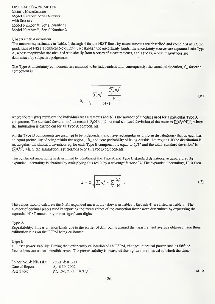
Uncertainty Assessment

The uncertainty estimates in Tables 1 through 4 for the NIST linearity measurements are described and combined using the

guidelines of NIST Technical Note 1297. To establish the uncertainty limits, the uncertainty sources are separated into Type

A, whose magnitudes are obtained statistically from a series of measurements, and Type B, whose magnitudes are

determined by subjective judgement.

The Type A imcertainty components are assumed to be independent and, consequently, the standard deviation, S^, for each

component is

NN-1

(6)

where the Xj values represent the individual measurements and N is the number of values used for a particular Type Acomponent. The standard deviation of the mean is S/N'^, and the total standard deviation of the mean is [£(Sr^/N)] ''', where

the summation is carried out for all Type A components.

All the Type B components are assumed to be independent and have rectangular or uniform distributions (that is, each has

an equal probability ofbeing within the region, ±6,, and zero probability of being outside that region). If the distribution is

rectangular, the standard deviation, o^, for each Type B component is equal to 6J3''^ and the total 'standard deviation' is

(L^s^)"^' where the summation is performed over all Type B components.

The combined uncertainty is determined by combining the Type A and Type B standard deviations in quadrature; the

expanded uncertainty is obtained by multiplying this result by a coverage factor of 2. The expanded uncertainty, U, is then

\ s r N

The values used to calculate the NIST expanded uncertainty (shown in Tables 1 through 4) are listed in Table 5. The

number of decimal places used in reporting the mean values of the correction factor were determined by expressing the

expanded NIST uncertainty to two significant digits.

Type ARepeatability: This is an uncertainty due to the scatter of data points around the measurement average obtained from three

calibration runs on the OFPM being calibrated.

TypeBa. Laser power stability: During the nonlinearity calibration of an OFPM, changes in optical power such as drift or

fluctuations can cause a possible error. The power stability is measured during the time interval in which the three


Date of Report:

Reference:

26000 & 81300

April 30, 2000

P.O. No. 2121 04/15/00

26



with Sensors



measurements are taken. The low power (when an individual shutter is open) is measured before and after the high power

(when both shutters are open). The value for laser stability is found by measuring the drift for each laser source. The slope

of the drift (percent per second) is then multiplied by the interval that the three shutters are open (3 s) during an actual

nonlinearity calibration. The maximum measured value of the power drift is 0.2 1 % at 850 nm, and 0.09 % at 1300 nm and

1550 nm. The standard uncertainty for laser stability is 0.21/(2/3) = 0.06 % at 850 nm, and 0.09/(2/3) = 0.03 % at 1300

nm and 1550 nm.

b. Polynomial truncation: The conversion fimction of an OFPM is a least-squares fit to a third-order polynomial. The

uncertainty is due to truncation of the polynomial of higher orders. The maximum value of the error is equal to 0.007 %.

The standard uncertainty is 0.007/(2/3) = 0.002 %.

c. Test meter sp>ectral responsivity: This uncertainty is caused by drift of the source wavelength and a drift of the optical

spectrum analyzer during each triplet measurement. The size of the uncertainty depends on the absorbing material of the

power meter detector. The value is estimated based on the spectral responsivity curves for Si, Ge, and InGaAs detectors.

We assimie a combined variation for the lasers wavelengths and accuracy of the optical spectrum analyzer of 0. 1 run.

d. Equation approximation: This imcertainty is due to the approximation in the nonlinearity equation. The uncertainty is

of second-order in magnitude, i.e., if the nonlinearity is 1 %, then the uncertainty is (0.01)^ or 10"^. This imcertainty

depends on the value for the nonlinearity in each case. The maximum uncertainty will be divided by (2/3).

e. Polarization: This uncertainty is due to effects caused by changes in polarization of the incident power during each

triplet measurement set. This uncertainty is related to polarization dependent loss (PDL) of the nonlinearity system.

Polarization uncertainty of the nonlinearity system is assumed to be small because we take a large number of measurements

(810 measurements per one power range) and because measxu^ment time scales are short compared to changes in the

system polarization state. The PDL of the nonlinearity system was measiu-ed using a random-polarization generator. The

maximum value of the system PDL is 0.002 dB or 0.05 %. The standard uncertainty is 0.05/(2/3) = 0.014 %.

Table 5 lists typical measurement uncertainties associated with the nonlinearity calibration of an OFPM. The exact value of

these various components can change depending on the particular measiuement conditions.

Folder No. & NISTK):

Date of Report:

Reference:

26000 & 81300

April 30, 2000

P.O. No. 2121 04/15/00 8 of 10

27


Model Niunber, Serial Number

with Sensors



Table 5. Typical nonlinearity measurement uncertainties.

Soiu-ce Standard uncertainty (type)

(%)

Laser stability

@ 850 nm 0.06 (B)

@ 1300 & 1550 nm 0.03 (B)



@850nm(Si) 0.004(B)

@ 850 nm(Ge) 0.014(B)

@ 850 nm anGaAs) 0.015(B)

@ 1300 nm (Ge) 0.004 (B)

@ 1300 nm (InGaAs) 0.003 (B)

@ 1550 nm (Ge) 0.027 (B)

@ 1550 nm (InGaAs) 0.001 (B)

Polarization ^ 0.014(B)

Equation approximation 0.003 (B)

Repeatability (N = 3) See Tables 1 through 4 (A)

Typical combined uncertainty 0.05

Typical expanded uncertainty (k = 2) 0. 10

Folder No. & NISTID: 26000 & 8 1300



28



with Sensors



For the Director, Report Reviewed By:

National Institute of Standards

and Technology

Gordon W. Day, Division Chief Thomas R. Scott, Group Leader

Optoelectronics Division Sources and Detectors Group


Report Reviewed By Report Prepared/Calibrated By:

Christopher L. Cromer, Project Leader

Sources and Detectors Group


Igor Vayshenker, Electronics Engineer

Sources and Detectors Group



Date of Report:

Reference:

26000 & 81300

April 30, 2000

P.O. No. 2121 04/15/00 10 of 10

29

THE SP 250 SERIES ON NIST MEASUREMENT SERVICES*

SP 250-1 Spectral Radiance Calibrations

PB871 79883

SP 250-2 Far Ultraviolet Detector Standards

PB87227609

SP 250-3 Radiometric Standards in the Vacuum Ultraviolet

PB87227625

SP 250-4 Fricke Dosimetry in Higti-Energy Electron BeamsPB881 10374

SP 250-5 Alptia-Particle Calibrations

PB88168620

SP 250-6 Regular Spectral Transmittance

PB881 08550

SP 250-7 Radiance Temperature Calibrations

PB881 23674

SP 250-8 Spectral Reflectance

PB881 09905

SP 250-9 Calibration of Beta-Particle-Emitting Ophthalmic

Applicators

PB881 08535

SP 250-10 Radioactivity Calibrations with the "4tt" GammaIonization Chamber and Other Radioactivity

Calibration Capabilities

PB88123708

SP 250-1 1 Dosimetry for High Dose Applications

PB88201587

SP 250-12 Neutron Personnel Dosimetry

PB87227617

SP 250-13 Activation Foil Irradiation with Californium

Fission Sources

PB882 17443

SP 250-14 Activation Foil Irradiation by Reactor Cavity

Fission Sources

PB882 17435

SP 250-15 Photometric Calibrations

PB881 53747

SP 250-1 6 Calibration of X-Ray and Gamma-RayMeasuring Instruments

PB88211826

SP 250-17 The NBS Photodetector Spectral ResponseCalibration Transfer Program

PB88201595

SP 250-1 8 Neutron Source Strength Calibrations

PB88211818

SP 250-19 Calibration of Gamma-Ray-Emitting

Brachytherapy Sources

PB89 193858

SP 250-20 Spectral Irradiance Calibrations

PB881 23781

SP 250-21 Calibration of Beta-Particle Radiation

Instrumentation

PB88201579

SP 250-22 Platinum Resistance Thermometer Calibrations

PB881 38367

SP 250-23 Liquid-in-Glass Thermometer Calibration Service

PB891 28888

SP 250-24 Standard Cell Calibrations

PB881 23690

SP 250-25 Calibration Service for Inductive

Voltage Dividers

SP 250-26 NBS Phase Angle Calibration Services

PB88225636

SP 250-27 AC-DC Difference Calibrations

PB892222616

SP 250-28 Solid-state DC Voltage Standard Calibrations

PB881 68703

SP 250-29 Traceable Frequency Calibrations

PB881 68364

SP 250-30 GOES Satellite Time Code Dissemination:

Description and Operation

PB881 68760

SP 250-31 Mass Calibrations

PB891 53894

SP 250-32 A Calibration Service for 30 MHz Attenuation

and Phase Shift

PB88238324

SP 250-33 A Calibration Service for Voltage Transformers

and High-Voltage Capacitors

PB882252903

SP 250-34 High Vacuum Standard and Its UsePB891 93841

SP 250-35 The Calibration of Thermocouples

and Thermocouple Materials

PB89209340

SP 250-36 A Calibration Service for Current Transformers

PB91216770

SP 250-37 Photometric Calibrations

PB97 148472

SP 250-38 NIST Leak Calibration Service

PB92 149772

SP 250-39 NIST Pressure Calibration Service

PB94 164043

SP 250-40 Absorbed-Dose Calibration of Ionization Chambersin a "^"Co Gamma-Ray BeamSN003-003-03034-1 $2.00

SP 250-41 Spectroradiometric Detector Measurements:

Part I- Ultraviolet Detectors and

Part II - Visible to Near-Infrared Detectors

SN003-003-03550-5 $9.50

SP 250-42 Sprectroradiometric Detector Measurements:

Part III—Infrared Detectors

SN003-003-03582-3 $5.25

SP 250-43 Radiance Temperature Calibrations

SN003-003-03511-4 $10.00

SP 250-44 Radiation Processing Dosimetry Calibration

Services and Measurement Assurance Program

SN003-003-03513-1

* Entries containing a stock number (SN003-003-) and price can be purchased from the Superintendent of Documents, U.S. GovernmentPrinting Office, Washington, DC 20402-9325. GPO will accept checks, money orders, VISA, and MasterCard. For more infomation, or to place

an order, call (202) 512-1800. Be sure to cite the stock number on all orders.

Entries containing PB numbers can be purchased from the National Technical Information Service, Springfield, VA 221 61 . NTIS will accept

American Express in addition to the payment methods listed for GPO. For more information call (703)487-4650; to place an order call

(800) 553-6487. Fax: (703) 321-8547. Be sure to cite the PB number on all orders.

Entries without stock or PB numbers are in preparation.

THE SP 250 SERIES ON NIST MEASUREMENT SERVICES* - Continued

SP 250^5

SP 250-46

SP 250-47

SP 250^8

SP 250-49

Radiation Processing Dosimetry Calibration

Services: Manual of Calibration Procedures

SN003-003-03514-9 $4.00

NIST Multifunction Calibration System

SN003-003-03515-7 $2.75

NIST Calibration Service for Capacitance

Standards at Low Frequencies

SN003-003-03549-1 $7.00

Spectral Reflectance

SN003-003-03545-9 $14.00

NIST Calibration Services for Gas Flow

Meters: Piston Prover and Bell Prover

Gas Flow Facilities

SN003-003-03560-2 $6.00

SP 250-51 Calibration Service of Optoelectronic

Frequency Response at 1319 nm for

Combined Photodiode/rf Power Sensor

Transfer Standards

SN003-003-03623-4

SP 250-52 Error Analysis and Calibration Uncertainty of

Capacitance Standards at NIST

SP 250-53 Calibration Service for Spectral Responsivity of

Laser and Optical-Fiber Power Meters at

Wavelengtfis Between 0.4 (jim and 1 .8 pim

SN003-003-03624-2

SP 250-54 Optical Fiber Power Meter Calibrations at NIST

SP 250-56 Optical Fiber Power Meter Nonlinearity Calibrations

at NIST

* Entries containing a stock number (SN003-003-) and price can be purctnased from the Superintendent of Documents, U.S. GovernmentPrinting Office, Washiington, DC 20402-9325. GPO will accept checks, money orders, VISA, and MasterCard. For more infomation, or to place

an order, call (202) 512-1800. Be sure to cite the stock number on all orders.

Entries containing PB numbers can be purchased from the National Technical Information Service, Springfield, VA 22161. NTIS will accept

American Express in addition to the payment methods listed for GPO. For more information call (703)487-4650; to place an order call

(800) 553-6487. Fax: (703) 321-8547. Be sure to cite the PB number on all orders.

Entries without stock or PB numbers are in preparation.

NISTiTechnical Publications

Periodical

Journal of Research of the National Institute of Standards and Technology—Reports NIST research and

development in those disciplines of the physical and engineering sciences in which the Institute is active.

These include physics, chemistry, engineering, mathematics, and computer sciences. Papers cover a broad

range of subjects, with major emphasis on measurement methodology and the basic technology underlying

standardization. Also included from time to time are survey articles on topics closely related to the Institute's

technical and scientific programs. Issued six times a year.

Nonperiodicais

Monographs—Major contributions to the technical literature on various subjects related to the Institute's

scientific and technical activities.

Handbooks—Recommended codes of engineering and industrial practice (including safety codes) developed

in cooperation with interested industries, professional organizations, and regulatory bodies.

Special Publications—Include proceedings of conferences sponsored by NIST NIST annual reports, andother special publications appropriate to this grouping such as wall charts, pocket cards, and bibliographies.

National Standard Reference Data Series—Provides quantitative data on the physical and chemical

properties of materials, compiled from the world's literature and critically evaluated. Developed under aworldwide program coordinated by NIST under the authority of the National Standard Data Act (Public Law90-396). NOTE: The Journal of Physical and Chemical Reference Data (JPCRD) is published bi-monthly for

NIST by the American Chemical Society (ACS) and the American Institute of Physics (AlP). Subscriptions,

reprints, and supplements are available from ACS, 1 155 Sixteenth St., NW, Washington, DC 20056.

Building Science Series—Disseminates technical information developed at the Institute on building

materials, components, systems, and whole structures. The series presents research results, test methods,

and performance criteria related to the structural and environmental functions and the durability and safety

characteristics of building elements and systems.

Technical Notes—Studies or reports which are complete in themselves but restrictive in their treatment of asubject. Analogous to monographs but not so comprehensive in scope or definitive in treatment of the

subject area. Often serve as a vehicle for final reports of work performed at NIST under the sponsorship of

other government agencies.

Voluntary Product Standards—Developed under procedures published by the Department of Commerce in

Part 10, Title 15, of the Code of Federal Regulations. The standards establish nationally recognized

requirements for products, and provide all concerned interests with a basis for common understanding of the

characteristics of the products. NIST administers this program in support of the efforts of private-sector

standardizing organizations.

Order the following NIST publications—FIPS and NISTIRs—from the National Technical

Information Service, Springfield, VA 22161.

Federal Information Processing Standards Publications (FIPS PUB)—Publications in this series collectively

constitute the Federal Information Processing Standards Register. The Register serves as the official source

of information in the Federal Government regarding standards issued by NIST pursuant to the Federal

Property and Administrative Services Act of 1949 as amended. Public Law 89-306 (79 Stat. 1127), and as

implemented by Executive Order 11717 (38 FR 12315, dated May 11, 1973) and Part 6 of Title 15 CFR(Code of Federal Regulations).

NIST Interagency Reports (NISTIR)—A special series of interim or final reports on work performed by NISTfor outside sponsors (both government and nongovernment). In general, initial distribution is handled by the

sponsor; public distribution is by the National Technical Information Service, Springfield, VA 22161, in paper

copy or microfiche form.

0)o

£Ê ô-g" 1O CO4-" >*rc o

E I

Q.—

Si. o

3 Z

00CMCOCO

I

COoCOo

o 5 Oc -o Of; -O o0) il <u

I— CD :o

T3 in 5ro CO CD

ooCO

a>M3

(A Q)

0) 5c Ew D.3 ,_m £TO ^'o w

O Q.