Embed Size (px)
Citation preview
www.iap.uni-jena.de
Optical Design with Zemax
for PhD - Basics
Lecture 1: Introduction
2015-10-26
Herbert Gross
Winter term 2015

2
Preliminary Schedule
No Date Subject Detailed content
1 26.10. Introduction
Zemax interface, menus, file handling, system description, editors, preferences,
updates, system reports, coordinate systems, aperture, field, wavelength, layouts,
raytrace, diameters, stop and pupil, solves, ray fans, paraxial optics
2 02.11. Basic Zemax handling surface types, quick focus, catalogs, vignetting, footprints, system insertion, scaling,
component reversal
3 09.11. Properties of optical systems aspheres, gradient media, gratings and diffractive surfaces, special types of
surfaces, telecentricity, ray aiming, afocal systems
4 16.11. Aberrations I representations, spot, Seidel, transverse aberration curves, Zernike wave
aberrations
5 23.11. Aberrations II PSF, MTF, ESF
6 30.11. Optimization I algorithms, merit function, variables, pick up’s
7 07.12. Optimization II methodology, correction process, special requirements, examples
8 14.12. Advanced handling slider, universal plot, I/O of data, material index fit, multi configuration, macro
language
9 04.01. Imaging Fourier imaging, geometrical images
10 11.01. Correction I simple and medium examples
11 18.01. Correction II advanced examples
12 25.01. Illumination simple illumination calculations, non-sequential option
13 01.02. Physical optical modelling Gaussian beams, POP propagation
14 08.02. Tolerancing Sensitivities, Tolerancing, Adjustment
1. Introduction
2. Zemax interface, menues, file handling, preferences
3. Editors, updates, windows, preferences
4. Coordinate systems and notations
5. System description, reports
6. Component reversal, system insertion, scaling
7. Solves and pickups, variables
8. 3D geometry
9. Aperture, field, wavelength
10. Glass catalogs
11. Raytrace
12. Layouts
3
Content

Modelling of Optical Systems
Principal purpose of calculations:
System, data of the structure(radii, distances, indices,...)
Function, data of properties,
quality performance(spot diameter, MTF, Strehl ratio,...)
Analysisimaging
aberration
theorie
Synthesislens design
Ref: W. Richter
Imaging model with levels of refinement
Analytical approximation and classification
(aberrations,..)
Paraxial model
(focal length, magnification, aperture,..)
Geometrical optics
(transverse aberrations, wave aberration,
distortion,...)
Wave optics
(point spread function, OTF,...)
with
diffractionapproximation
--> 0
Taylor
expansion
linear
approximation
4

Five levels of modelling:
1. Geometrical raytrace with analysis
2. Equivalent geometrical quantities,
classification
3. Physical model:
complex pupil function
4. Primary physical quantities
5. Secondary physical quantities
Blue arrows: conversion of quantities
Modelling of Optical Systems
ray
tracing
optical path
length
wave
aberration W
transverse
aberrationlongitudinal aberrations
Zernike
coefficients
pupil
function
point spread
function (PSF)
Strehlnumber
optical
transfer function
geometricalspot diagramm
rms
value
intersectionpoints
final analysis reference ray in
the image space
referencesphere
orthogonalexpansion
analysis
sum of
coefficientsMarechal
approxima-
tion
exponentialfunction
of the
phase
Fourier
transformLuneburg integral
( far field )
Kirchhoffintegral
maximum
of the squared
amplitude
Fouriertransformsquared amplitude
sum of
squaresMarechalapproxima-
tion
integration ofspatial
frequencies
Rayleigh unit
equivalencetypes of
aberrationsdifferen
tiationinte-
gration
full
aperture
single types of aberrations
definition
geometricaloptical
transfer function
Fouriertransform
approximation
auto-correlationDuffieux
integral
resolution
threshold value spatial frequency
threshold value spatial
frequency approximationspot diameter
approximation diameter of the
spot
Marechalapproximation
final analysis reference ray in the image planeGeometrical
raytrace
with Snells law
Geometrical
equivalents
classification
Physical
model
Primary
physical
quantities
Secondary
physical
quantities
5

There are 4 types of windows in Zemax:
1. Editors for data input:
lens data, extra data, multiconfiguration, tolerances
2. Output windows for graphical representation of results
Here mostly setting-windowss are supported to optimize the layout
3. Text windows for output in ASCII numerical numbers (can be exported)
4. Dialog boxes for data input, error reports and more
There are several files associates with Zemax
1. Data files (.ZMX)
2. Session files (.SES) for system settings (can be de-activated)
3. Glass catalogs, lens catalogs, coating catalogs, BRDF catalogs, macros,
images, POP data, refractive index files,...
There are in general two working modes of Zemax
1. Sequential raytrace (or partial non-sequencial)
2. Non-sequential
Zemax Interface
6

Helpful shortcuts:
1. F3 undo
2. F2 edit a cell in the editor
3. cntr A multiconfiguration toggle
4. cntr V variable toggle
5. F6 merit function editor
6. cntr U update
7. shift cntr Q quick focus
Window options:
1. several export options
2. fixed aspect ratios
3. clone
4. adding comments or graphics
Zemax Interface
7

Coordinate systems
2D sections: y-z shown
Sign of lengths, radii, angles:
z / optical axis
y / meridional section
tangential plane
x / sagittal plane
+ s- s
negative:
to the left
positive:
to the right+ R
+ j
reference
angle positive:
counterclockwise
+ R1
negative:
C to the leftpositive:
C to the right
- R2
C1C2
Coordinate Systems and Sign of Quantities
8

Interface surfaces
- mathematical modelled surfaces
- planes, spheres, aspheres, conics, free shaped surfaces,…
Size of components
- thickness and distances along the axis
- transversal size,circular diameter, complicated contours
Geometry of the setup
- special case: rotational symmetry
- general case: 3D, tilt angles, offsets and decentrations, needs vectorial approach
Materials
- refractive indices for all used wavelengths
- other properties: absorption, birefringence, nonlinear coefficients, index gradients,…
Special surfaces
- gratings, diffractive elements
- arrays, scattering surfaces
9
Description of Optical Systems

Single step:
- surface and transition
- parameters: radius, diameter, thickness,
refractive index, aspherical constants,
conic parameter, decenter, tilt,...
Complete system:
- sequence of surfaces
- object has index 0
- image has index N
- tN does not exist
Ray path has fixed
sequence
0-1-2-...-(N-1)-N surface
index
object
plane
1
0 2
image
plane
N-23 j N-1.... .... N
0
1
2 3 j N-2 N-1 (N)
thickness
index
surfaces
surface j
medium j
tj / nj
radius rj
diameter Dj
System Model
10

Menu: Reports / Prescription
data
Menu:
reports / prescription data
System Data Tables
11

System Data Tables
12

Necessary data for system calculation:
1. system surfaces with parameters (radius)
2. distances with parameters (length, material)
3. stop surface
4. wavelength(s)
5. aperture
6. field point(s)
Optional inputs:
1. finite diameters
2. vignetting factors
3. decenter and tilt
4. coordinate reference
5. weighting factors
6. multi configurations
7. ...
System data
13

Useful commands for system changes:
1. Scaling (e.g. patents)
2. Insert system
with other system file
File - Insert Lens
2. Reverse system
14
System Changes

Setting of surface properties
local tilt
and
decenterdiameter
surface type
additional drawing
switches
coatingoperator and
sampling for POP
scattering
options
Surface Properties and Settings
15

Value of the parameter dependents on other requirement
Pickup of radius/thickness: linear dependence on other system parameter
Determined to have fixed: - marginal ray height
- chief ray angle
- marginal ray normal
- chief ray normal
- aplanatic surface
- element power
- concentric surface
- concentric radius
- F number
- marginal ray height
- chief ray height
- edge thickness
- optical path difference
- position
- compensator
- center of curvature
- pupil position
Solves
16

Examples for solves:
1. last radius forces given image aperture
2. get symmetry of system parts
3. multiple used system parts
4. moving lenses with constant system length
5. bending of a lens with constant focal length
6. non-negative edge thickness of a lens
7. bending angle of a mirror (i'=i)
8. decenter/tilt of a component with return
Solves
17

Open different menus with a right-mouse-click in the corresponding editor cell
Solves can be chosen individually
Individual data for every surface in this menu
Solves
18

General input of tilt and decenter:
Coordinate break surface
Change of coordinate system with lateral translation and 3 rotations angles
Direct listing in lens editor
Not shown in layout drawing
19
3D Geometry

Auxiliary menus:
1. Tilt/Decenter element
2. Folding mirror
20
3D Geometry

Local tilt and decenter of a surface
1. no direct visibility in lens editor
only + near surface index
2. input in surface properties
3. with effect on following system surfaces
21
3D Geometry

Imaging on axis: circular / rotational symmetry
Only spherical aberration and chromatical aberrations
Finite field size, object point off-axis:
- chief ray as reference
- skew ray bundels:
coma and distortion
- Vignetting, cone of ray bundle
not circular symmetric
- to distinguish:
tangential and sagittal
plane
O
entrance
pupil
y yp
chief ray
exit
pupil
y' y'p
O'
w'
w
R'AP
u
chief ray
object
planeimage
plane
marginal/rim
ray
u'
Definition of Aperture and Field
22

Quantitative measures of relative opening / size of accepted light cone
Numerical aperture
F-number
Approximation for small
apertures:
'sin unNA
EXD
fF
'#
NAF
2
1#
image
plane
marginal ray
exit
pupil
chief ray
U'W'
DEX
f'
Aperture Definition
23

The physical stop defines
the aperture cone angle u
The real system may be complex
The entrance pupil fixes the
acceptance cone in the
object space
The exit pupil fixes the
acceptance cone in the
image space
uobject
image
stop
EnP
ExP
object
image
black box
details complicated
real
system
? ?
Ref: Julie Bentley
Optical system stop
24
Relevance of the system pupil :
Brightness of the image
Transfer of energy
Resolution of details
Information transfer
Image quality
Aberrations due to aperture
Image perspective
Perception of depth
Compound systems:
matching of pupils is necessary, location and size
Properties of the pupil
25

exit
pupil
upper
marginal ray
chief
ray
lower coma
raystop
field point
of image
UU'
W
lower marginal
ray
upper coma
ray
on axis
point of
image
outer field
point of
object
object
point
on axis
entrance
pupil
Entrance and exit pupil
26

Cardinal Points of a Lens
P'
s'P'
Real lenses:
The surface with the principal points
as apparent ray bending points is a
curved shell
The ideal principal plane exists only
in the paraxial approximation
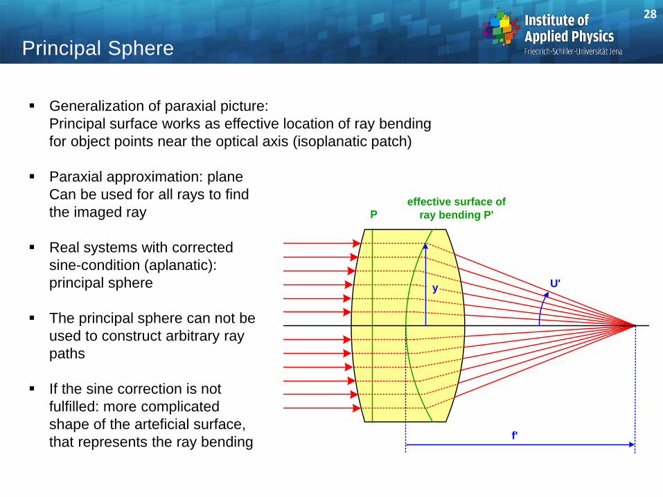
Generalization of paraxial picture:
Principal surface works as effective location of ray bending
for object points near the optical axis (isoplanatic patch)
Paraxial approximation: plane
Can be used for all rays to find
the imaged ray
Real systems with corrected
sine-condition (aplanatic):
principal sphere
The principal sphere can not be
used to construct arbitrary ray
paths
If the sine correction is not
fulfilled: more complicated
shape of the arteficial surface,
that represents the ray bending
Principal Sphere
effective surface of
ray bending P'
y
f'
U'
P
28

The principal planes in paraxial optics are defined as the locations of the apparent ray bending
of a lens of system
In the case of a system with corrected sine conditions, these surfaces are spheres
Sine condition and pupil spheres are also limited for off-axis points near to the optical axis
For object points far from the axis, the apparent locations are complicated surfaces, which
may consist of two branches
29
Limitation of Principal Surface Definition

Different possible options for specification of the aperture in Zemax:
1. Entrance pupil diameter
2. Image space F#
3. Object space NA
4. Paraxial working F#
5. Object cone angle
6. Floating by stop size
Stop location:
1. Fixes the chief ray intersection point
2. input not necessary for telecentric object space
3. is used for aperture determination in case of aiming
Special cases:
1. Object in infinity (NA, cone angle input impossible)
2. Image in infinity (afocal)
3. Object space telecentric
Aperture data in Zemax
30

3D-effects due to vignetting
Truncation of the at different surfaces for the upper and the lower part
of the cone
Vignetting
object lens 1 lens 2 imageaperture
stop
lower
truncation
upper
truncation
sagittal
trauncation
chief
ray
coma
rays
31

Truncation of the light cone
with asymmetric ray path
for off-axis field points
Intensity decrease towards
the edge of the image
Definition of the chief ray:
ray through energetic centroid
Vignetting can be used to avoid
uncorrectable coma aberrations
in the outer field
Effective free area with extrem
aspect ratio:
anamorphic resolution
projection of the
rim of the 2nd lens
projection of the
rim of the 1st lens
Projektion der
Aperturblende
free area of the
aperture
sagittal
coma rays
meridional
coma rayschief
ray
Vignetting
32

1. Determination of one surface as system stop:
- Fixes the chief ray intersection point with axis
- can be set in surface properties menu
- indicated by STO in lens data editor
- determines the aperture for the option 'float by stop size'
2. Diameters in lens data editor
- indicated U for user defined
- only circular shape
- effects drawing
- effects ray vignetting
- can be used to draw 'nice lenses' with
overflow of diameter
3. Diameters as surface properties:
- effects on rays in drawing (vignetting)
- no effect on lens shapes in drawing
- also complicated shapes and decenter
possible
- indicated in lens data editor by a star
33
Diameters and stop sizes
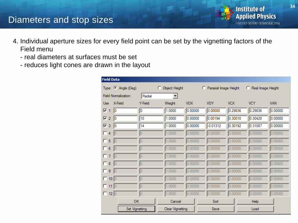
4. Individual aperture sizes for every field point can be set by the vignetting factors of the
Field menu
- real diameters at surfaces must be set
- reduces light cones are drawn in the layout
34
Diameters and stop sizes

Important types of optical materials:
1. Glasses
2. Crystals
3. Liquids
4. Plastics, cement
5. Gases
6. Metals
Optical parameters for characterization of materials
1. Refractive index, spectral resolved n()
2. Spectral transmission T()
3. Reflectivity R
4. Absorption
5. Anisotropy, index gradient, eigenfluorescence,…
Important non-optical parameters
1. Thermal expansion coefficient
2. Hardness
3. Chemical properties (resistence,…)
Optical materials
35

in [nm] Name Color Element
248.3 UV Hg
280.4 UV Hg
296.7278 UV Hg
312.5663 UV Hg
334.1478 UV Hg
365.0146 i UV Hg
404.6561 h violett Hg
435.8343 g blau Hg
479.9914 F' blau Cd
486.1327 F blau H
546.0740 e grün Hg
587.5618 d gelb He
589.2938 D gelb Na
632.8 HeNe-Laser
643.8469 C' rot Cd
656.2725 C rot H
706.5188 r rot He
852.11 s IR Cä
1013.98 t IR Hg
1060.0 Nd:YAG-Laser
Test wavelengths
36

refractive
index n
1.65
1.6
1.5
1.8
1.55
1.75
1.7
BK7
SF1
0.5 0.75 1.0 1.25 1.751.5 2.0
1.45
Flint
Kron
Description of dispersion:
Abbe number
Visual range of wavelengths:
Typical range of glasses
ne = 20 ...120
Two fundamental types of glass:
Crone glasses:
n small, n large
Flint glasses
n large, n small
n
n
n nF C
1
' '
ne
e
F C
n
n n
1
' '
Dispersion and Abbe number
37

Material with different dispersion values:
- Different slope and curvature of the dispersion curve
- Stronger change of index over wavelength for large dispersion
- Inversion of index sequence at the boundaries of the spectrum possible
refractive index n
F6
SK18A
1.675
1.7
1.65
1.625
1.60.5 0.75 1.0 1.25 1.751.5 2.0
VIS
flint
n small
slope large
crown
n largeslope small
Dispersion
38

Schott formula
empirical
Sellmeier
Based on oscillator model
Bausch-Lomb
empirical
Herzberger
Based on oscillator model
Hartmann
Based on oscillator model
n a a a a a ao + + + + +
1
2
2
2
3
4
4
6
5
8
n A B C( )
+
+
2
212
2
222
n A B CD E
Fo
o
( )
( )
+ + + +
+
2 4
2
2
2 22
2 2
mmit
aaaan
o
oo
o
168.0
)(222
3
22
22
1
+
++
+
+
5
4
3
1)(a
a
a
aan o
Dispersion formulas
39

Relative partial dispersion :
Change of dispersion slope with
Definition of local slope for selected
wavelengths relative to secondary
colors
Special selections for characteristic
ranges of the visible spectrum
= 656 / 1014 nm far IR
= 656 / 852 nm near IR
= 486 / 546 nm blue edge of VIS
= 435 / 486 nm near UV
= 365 / 435 nm far UV
P
n n
n nF C
1 2
1 2
' '
n
400 600 800 1000700500 900 1100
e : 546 nm
main color
F' : 480 nm
1. secondary
color
g : 435 nmUV edge
C' : 644 nm
s : 852 nm
IR edge
t : 1014 nm
IR edge
C : 656 nmF : 486 nm
d : 588 nm
i : 365 nm
UV edge
i - g
F - C
C - s
C - t
F - e
g - F
2. secondary
color
1.48
1.49
1.5
1.51
1.52
1.53
1.54
n()
Relative partial dispersion
40

Usual representation of
glasses:
diagram of refractive index
vs dispersion n(n)
Left to right:
Increasing dispersion
decreasing Abbe number
Glass diagram
41

Selection of glass catalogs in
GENERAL / GLASS CATALOGS
Viewing of dispersion curves
ANALYSIS / GLASS AND GRADIENT
Viewing of glass map
42
Glasses in Zemax

Viewing of transmission curves
also for several glasses in comparison
ANALYSIS / GLASS AND GRADIENT
Definition of a glass as a variable point in the
map (model glass)
43
Glasses in Zemax

zoptical
axis
y j
u'j-1
ij
dj-1
ds j-1
ds j
i'j
u'j
n j
nj-1
mediummedium
surface j-1
surface j
ray
dj
vertex distance
oblique thickness
rr
Ray: straight line between two intersection points
System: sequence of spherical surfaces
Data: - radii, curvature c=1/r
- vertex distances
- refractive indices
- transverse diameter
Surfaces of 2nd order:
Calculation of intersection points
analytically possible: fast
computation
44
Scheme of raytrace

yj
z
Pj+1
sj
xj
yj+1
xj+1
Pj
surface
No j
surface
No j+1
dj sj+1
intersection
point
ej
normal
vector
ej+1
ray
distance
intersection
point
normal
vector
General 3D geometry
Tilt and decenter of surfaces
General shaped free form surfaces
Full description with 3 components
Global and local coordinate systems
45
Vectorial raytrace

Vignetting/truncation of ray at finite sized diameter:
can or can not considered (optional)
No physical intersection point of ray with surface
Total internal reflection
Negative edge thickness of lenses
Negative thickness without mirror-reflection
Diffraction at boundaries
index
j
index
j+1
axis
negative
un-physical
regular
irregular
axis
no intersection
point
axis
intersection:
- mathematical possible
- physical not realized
axis
total
internal
reflection
Raytrace errors
46

Definition of a single ray by two points
First point in object plane:
relative normalized coordinates: Hx, Hy
Second point in entrance pupil plane:
relative normalized coordinates Px, Py
Single Ray Selection
axis
x p
pupil plane
object plane
x
y
first point
yp
second point
HyHx
Py
Px
47

Meridional rays:
in main cross section plane
Sagittal rays:
perpendicular to main cross
section plane
Coma rays:
Going through field point
and edge of pupil
Oblique rays:
without symmetry
Special rays in 3D
axis
y
x
p
p
pupil plane
object plane
x
y
axissagittal ray
meridional marginal ray
skew raychief ray
sagittal coma ray
upper meridional coma ray
lower meridional coma ray
field point
axis point
48

Off-axis object point:
1. Meridional plane / tangential plane / main cross section plane
contains object point and optical axis
2. Sagittal plane:
perpendicular to meridional plane through object point
x
y
x'
y'
z
lens
meridional
plane
sagittal
plane
object
planeimage
plane
Tangential and sagittal plane
49

Ray fan:
2-dimensional plane set of rays
Ray cone:
3-dimensional filled ray cone
object
point
pupil
grid
Ray fans and ray cones
50

Pupil sampling for calculation of transverse aberrations:
all rays from one object point to all pupil points on x- and y-axis
Two planes with 1-dimensional ray fans
No complete information: no skew rays
y'p
x'p
yp
xp x'
y'
z
yo
xo
object
plane
entrance
pupil
exit
pupil
image
plane
tangential
sagittal
Pupil sampling
51

Pupil sampling in 3D for spot diagram:
all rays from one object point through all pupil points in 2D
Light cone completly filled with rays
y'p
x'p
yp
xp x'
y'
z
yo
xo
object
plane
entrance
pupil
exit
pupil
image
plane
Sampling of pupil area
52

Pupil Sampling
53
polar grid cartesian isoenergetic circular
hexagonal statistical pseudo-statistical (Halton)
Fibonacci spirals
Criteria: 1. iso energetic rays 2. good boundary description 3. good spatial resolution

Artefacts due to regular gridding of the pupil of the spot in the image plane
In reality a smooth density of the spot is true
The line structures are discretization effects of the sampling
hexagonal statisticalcartesian
Artefacts of pupil sampling
54

Selection of 2 points on the ray on object and entrance pupil plane
Real and paraxial rays are tabulated
Coordinate reference can be selected to be local or global
55
Raytrace in Zemax

Graphical control of system
and ray path
Principal options in Zemax:
1. 2D section for circular symmetry
2. 3D general drawing
Several options in settings
Zooming with mouse
56
Layout options

Different options for 3D case
Multiconfiguration plot possible
Rayfan can be chosen
57
Layout options

Professional graphic
Many layout options
Rotation with mouse or arrow buttons
58
Layout options

Looking for the ray bundle cross sections
59
Footprints