Optical Analysis of Strength Tests Based on Block-Matching Techniques

Computer-Aided Civil and Infrastructure Engineering 00 (2011) 1–21

Optical Analysis of Strength Tests Basedon Block-Matching Techniques

Alvaro Rodriguez∗

Department of Information and Communications Technologies, University of A Coruna, A Coruna, Spain

Juan R. Rabunal

Centre of Technological Innovation in Construction and Civil Engineering (CITEEC), University of A Coruna, A Coruna,Spain

Juan L. Perez

School of Building Engineering and Technical Architecture, University of A Coruna, A Coruna, Spain

&

Fernando Martınez-Abella

Department of Construction Technology, University of A Coruna, A Coruna, Spain

Abstract: One of the main issues in civil engineering isto analyze the behavior of materials in strength tests. Tra-ditionally, information about displacements and strainsin the materials is carried out from these tests using phys-ical devices such as strain gauges or other transducers.

Although these devices provide accurate and robustmeasurements in a wide range of situations, they are lim-ited to obtaining measurements in a single point of thematerial and in a single direction of the movement, thus,the global behavior of the material cannot be analyzed.

The proposed technique consists of the integration ofa calibration process with a block-matching algorithmto measure displacements from images. This algorithmuses the similarity between regions in the images to ex-tract the 2D vector displacement field from each point,and to quantify the strain on the surface of the material.

The proposed algorithm has been designed to mea-sure displacements from real images of material surfacestaken during strength tests, and it has the advantages ofbeing robust with long-range displacements, of perform-

∗To whom correspondence should be addressed. E-mail: [email protected].

ing the analysis on the image space domain (avoiding theproblems related to the use of Fourier Transforms), andof measurements in long sequences related to a real pointof the material and not to a pixel position.

1 INTRODUCTION

Some of the main needs in civil engineering are to knowthe stress–strain response of materials used in struc-tures, to evaluate their strength, and to determine theirbehavior during the design working life.

For this purpose, strength tests are usually carried outby applying controlled loads or strains to a test model (ascale model of reduced size, maintaining all the proper-ties of the material to be analyzed). The goal is to findout parameters such as material strength or displace-ment evolution, comparing real construction models totheoretical ones, or determining whether a given mate-rial is suitable for a particular use.

In these tests, information about the material be-havior is traditionally obtained using specific devices,such as strain gauges or linear variable differential

C© 2011 Computer-Aided Civil and Infrastructure Engineering.DOI: 10.1111/j.1467-8667.2011.00743.x

2 Rodriguez, Rabunal, Perez & Martınez-Abella

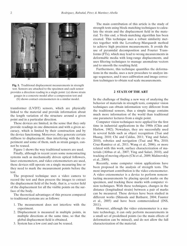
Fig. 1. Traditional displacement measurements in strengthtest. Sensors are attached to the specimen and each sensor

provides a direction reading in a single point: (a) shows straingauges in a concrete model after a compression test and

(b) shows contact extensometers in a similar model.

transformer (LVDT) sensors, which are physicallylinked to the material and provide information aboutthe length variation of the structure around a givenpoint and in a particular direction.

These devices are limited, in the sense that they onlyprovide readings in one dimension and with a given ac-curacy, which is limited by their construction and bythe device functioning. Moreover, they generate certainstiffness to displacement, thus interfering with the ex-periment and some of them, such as strain gauges, can-not be reused.

Figure 1 shows the way traditional sensors are used.Finally, although in recent years some noncontacting

systems such as mechanically driven optical followers,laser extensometers, and video extensometers are used,these devices still operate on a single measuring line orthey need to mark the measurement points before thetest.

The proposed technique uses a video camera torecord the test and then process the images to extractthe displacement field of the body, that is, a vector fieldof the displacement for all the visible points on the sur-face of the body.

The theoretical advantages of this process comparedto traditional systems are as follows:

1. The measurement does not interfere with theexperiment.

2. Displacement is measured in multiple points, inmultiple directions at the same time, so that theglobal displacement field is obtained.

3. System has a low cost and can be reused.

The main contribution of this article is the study ofstrength tests using block-matching techniques to calcu-late the strain and the displacement field in the mate-rial. To this end, a block-matching algorithm has beencreated. This technique uses a robust similarity met-rics together with the Levenberg–Marquardt methodto achieve high precision measurements. It avoids theuse of pyramidal decomposition and Fourier Trans-forms (FTs), which may lead to wrong measurements indeformable media with long-range displacements, anduses filtering techniques to manage anomalous vectorsand to smooth the resulting field.

Furthermore, this technique quantifies the deforma-tions in the media, uses a new procedure to analyze im-age sequences, and it uses calibration and image correc-tion techniques to obtain real scale measurements.

2 STATE OF THE ART

In the challenge of finding a new way of analyzing thebehavior of materials in strength tests, computer visiontechniques can obtain information very different fromthe traditional sensors, thus a simple image containsmuch more information of the world than traditionalone parameter lectures from a single point.

Computer vision techniques were applied for the firsttime in industrial applications in the 1980s (Chin andHarlow, 1982). Nowadays, they are successfully usedin several fields such as object recognition (Tsai andHuang, 2010; Chi and Caldas, 2011; Ying and Salari,2010), robotics and navigation (Tsai and Wu, 2010;Cruz-Ramırez et al., 2011; Wang et al., 2006), or morerelated with this work, surface characterization of ma-terials (Abbas et al., 2007; Ying and Salari, 2010), andtracking of moving objects (Chi et al., 2009; Malinovskiyet al., 2009).

Recently, some computer vision applications havebeen proposed in the analysis of strength tests. Themost important contribution is the video extensometer.A video extensometer is a device to perform noncon-tacting measurements by placing special marks on thespecimen, and tracking these marks with computer vi-sion techniques. With these techniques, changes in thedistance (longitudinal strain) between a pair of markscan be measured. These devices have been studied indifferent works (Shinoda and Bathurst, 2004; Fausteret al., 2005) and have been commercialized (INS,2011).

However, although the video extensometer is a ma-ture technology, it can only perform measurements ina small set of predefined points (so the main effects ofdeformation can be missed), and do not allow the fullcharacterization of the material.

Optical analysis of strength tests 3

The main difficulty for analyzing displacement innonrigid bodies from visual information is derived fromthe fact that the body geometry varies between two in-stants and thus, it is not possible to find out which partof the information characterizes the body, and can beused to estimate the displacement.

Traditional techniques for analyzing strain processesin computer vision are based on finding the parametersof a displacement model. Some additional knowledgeabout the model must be added to these procedures toobtain some robust measurements, considering nonrigidmovements. This knowledge typically consists of a setof well-known correspondence points, or estimating theequations regulating displacement d(i, j) (Bartoli, 2008;Pilet et al., 2007).

Optical flow techniques were carried out by Horn andSchunk (1981), and these are a field of computer visionfor displacement analysis. These techniques provide aflexible approach regarding the extraction of the motionfield of a scene without using any previous knowledgeabout the displacement of the objects in the image. Nev-ertheless, only very limited or too costly applications ofthese techniques have been found so far in the field ofcivil engineering (Chivers and Clocksin, 2000).

The works carried out in the flow-field analysis(Raffel et al., 2000; Raffel et al., 2007) showed that whenthe analyzed scene does not contain multiple objectswith different motions, a block-matching technique isthe most robust and flexible approach.

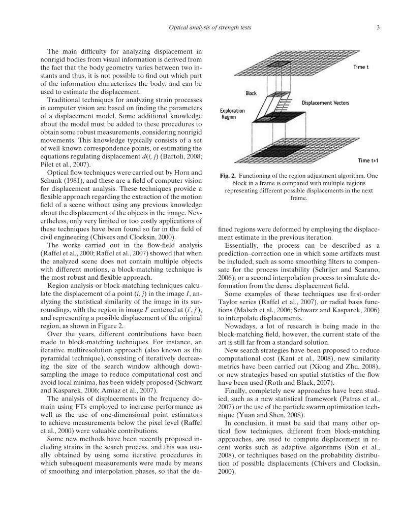
Region analysis or block-matching techniques calcu-late the displacement of a point (i, j) in the image I, an-alyzing the statistical similarity of the image in its sur-roundings, with the region in image I′ centered at (i′, j′),and representing a possible displacement of the originalregion, as shown in Figure 2.

Over the years, different contributions have beenmade to block-matching techniques. For instance, aniterative multiresolution approach (also known as thepyramidal technique), consisting of iteratively decreas-ing the size of the search window although down-sampling the image to reduce computational cost andavoid local minima, has been widely proposed (Schwarzand Kasparek, 2006; Amiaz et al., 2007).

The analysis of displacements in the frequency do-main using FTs employed to increase performance aswell as the use of one-dimensional point estimatorsto achieve measurements below the pixel level (Raffelet al., 2000) were valuable contributions.

Some new methods have been recently proposed in-cluding strains in the search process, and this was usu-ally obtained by using some iterative procedures inwhich subsequent measurements were made by meansof smoothing and interpolation phases, so that the de-

Fig. 2. Functioning of the region adjustment algorithm. Oneblock in a frame is compared with multiple regions

representing different possible displacements in the nextframe.

fined regions were deformed by employing the displace-ment estimate in the previous iteration.

Essentially, the process can be described as aprediction–correction one in which some artifacts mustbe included, such as some smoothing filters to compen-sate for the process instability (Schrijer and Scarano,2006), or a second interpolation process to simulate de-formation from the dense displacement field.

Some examples of these techniques use first-orderTaylor series (Raffel et al., 2007), or radial basis func-tions (Malsch et al., 2006; Schwarz and Kasparek, 2006)to interpolate displacements.

Nowadays, a lot of research is being made in theblock-matching field, however, the current state of theart is still far from a standard solution.

New search strategies have been proposed to reducecomputational cost (Kant et al., 2008), new similaritymetrics have been carried out (Xiong and Zhu, 2008),or new strategies based on spatial statistics of the flowhave been used (Roth and Black, 2007).

Finally, completely new approaches have been stud-ied, such as a new statistical framework (Patras et al.,2007) or the use of the particle swarm optimization tech-nique (Yuan and Shen, 2008).

In conclusion, it must be said that many other op-tical flow techniques, different from block-matchingapproaches, are used to compute displacement in re-cent works such as adaptive algorithms (Sun et al.,2008), or techniques based on the probability distribu-tion of possible displacements (Chivers and Clocksin,2000).


3 PROPOSED TECHNIQUE

3.1 General functioning

From the point of view of image processing, two instants(images) from the same scene are analyzed. The first im-age I may be considered as the input to a system whoseoutput generates the second image I′, separated from Iby a time interval �t.

The system transfer function H turns the entrance im-age I into the output one I′, and it is integrated by thedisplacement function d(i, j) plus a noise signal R.

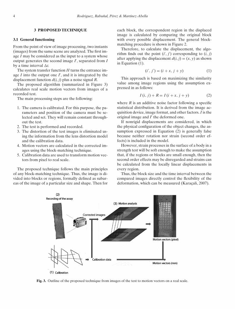
The proposed algorithm (summarized in Figure 3)calculates real scale motion vectors from images of arecorded test.

The main processing steps are the following:

1. The camera is calibrated. For this purpose, the pa-rameters and position of the camera must be se-lected and set. They will remain constant through-out the test.

2. The test is performed and recorded.3. The distortion of the test images is eliminated us-

ing the information from the lens distortion modeland the calibration data.

4. Motion vectors are calculated in the corrected im-ages using the block-matching technique.

5. Calibration data are used to transform motion vec-tors from pixel to real scale.

The proposed technique follows the main principlesof any block-matching technique. Thus, the image is di-vided into blocks or regions, formally defined as subar-eas of the image of a particular size and shape. Then for

each block, the correspondent region in the displacedimage is calculated by comparing the original blockwith every possible displacement. The general block-matching procedure is shown in Figure 2.

Therefore, to calculate the displacement, the algo-rithm finds out the point (i′, j′) corresponding to (i, j)after applying the displacement d(i, j) = (x, y) as shownin Equation (1).

(i ′, j ′) = (i + x, j + y) (1)

This approach is based on maximizing the similarityvalue among image regions using the assumption ex-pressed in as follows:

I (i, j) + R = I (i + x, j + y) (2)

where R is an additive noise factor following a specificstatistical distribution. It is derived from the image ac-quisition device, image format, and other factors. I is theoriginal image and I′ the deformed one.

If nonrigid displacements are considered, in whichthe physical configuration of the object changes, the as-sumption expressed in Equation (2) is generally falsebecause neither rotation nor strain (second order ef-fects) is included in the model.

However, strain processes in the surface of a body in astrength test will be soft enough to make the assumptionthat, if the regions or blocks are small enough, then thesecond order effects may be disregarded and strains canbe calculated from the locally linear displacements inevery region.

Thus, the block size and the time interval between thecompared images directly control the flexibility of thedeformation, which can be measured (Karacali, 2007).

Fig. 3. Outline of the proposed technique from images of the test to motion vectors on a real scale.


Concerning the block size, it may also be consid-ered that if the block size is too small, blocks will nothave enough information to estimate the correlationand wrong measurements can also be obtained. How-ever, small variations in the block size will not signifi-cantly affect the results.

A simple approach is used in this work to estimate ap-propriate size of the blocks. Thus, an approximate sizeof 16 × 16 pixels is used in small images, a size of 32 ×32 pixels is used in images bigger than 1 megapixel, and64 × 64 in images bigger than 5 megapixels.

However, block size may be adjusted to adapt it to im-age contents and recording conditions, such as the fieldof view (FOV), if they are very dissimilar to the blocksize used in this work.

At this point, it must be noted that the use of pyrami-dal techniques (although they have proven to be effec-tive in avoiding anomalous vectors and reducing com-putational complexity) may lead to an infringement ofthe locality principle explained before, and to achievingwrong measurements in presence of deformation. Thisis because of the fact that, pyramidal approaches down-sample the images (reducing the image size) althoughpreserving or enlarging the block size.

The proposed technique uses a flexible and direct ap-proach. The analysis is performed directly on the spacedomain with significant information, and avoiding thelimitations on block size and search range related tothe use of FTs. With this technique, valid data can onlybe achieved within a range of displacement of N/2 (N/4is recommended, N being a base two power region size)(Raffel et al., 2007).

Furthermore, because of the softness of the strains ex-pected, introducing second order effects is not required,and no further assumptions about the displacementin the scene have been made, improving in this waythe processing time and eliminating the interpolationerrors.

3.2 Displacement measurement

The algorithm employed in this work measures move-ment using the statistical similarity of the gray levels ineach region of the image. For this purpose, a region orblock is formally defined as a subarea of the image of aparticular and constant size and shape.

At this point, a similarity metrics, robust to naturalvariability processes in real images will be used to com-pute the most probable displacement for each point.This is important because of the natural changes in re-fraction in moving objects, changes in visual propertiesbecause of deformations, and the variability present incommon light sources.

The most popular metrics in image processing appli-cations are based on minimization of the mean square,or maximization of the correlation when information isprovided by gray levels rather than by local shapes andstructure (Zitova and Flusser, 2003).

Furthermore, the combination of different similar-ity techniques has been widely proposed (Arevalillo-Herraez et al., 2008; Wachs et al., 2009) where usuallythe registration parameters are weighted according tothe strength of each measure.

In this work, a metric called combined similarity met-ric (CSM), formed by a combination of the Pearson’scorrelation quotient (R), which is invariant to the aver-age of intensity for each block, and therefore robust toluminosity changes, and the mean squared error (MSE)has been used. This measure was proposed in (Moraleset al., 2005) and it is defined as follows:

CSM(Bi, j , B′i ′. j ′)

= R1 + k × MSE

=

∑N

((I (i, j) − μB) × (I ′ (i ′, j ′) − μB′))

N√∑N

(I (i, j) − μB)2

N×

∑N

(I ′ (i ′, j ′) − μB′)2

N

1 + k ×⎛⎝

∑N

(I (i, j) − I ′ (i ′, j ′))2

∑N

(I (i, j) − μB)

⎞⎠

(3)

where N is the size of the block, μB and μB′ are the av-erage intensity values of the two blocks compared (Bij,B′

i′,j′) which are centered in the points I(i, j) and I′(i′, j′),respectively, and k is a constant for weighing the MSEin the measurement, so that k = 0 → CSM = R.

This constant was empirically adjusted to k = 0.2using a training databank granted by Otago Univer-sity, New Zealand (GVRL, 2011), where the pro-posed metric shows a better performance than R andMSE.

The data obtained in the similarity analysis are a sta-tistical measurement of the most probable discrete dis-placement. However, the correlation value itself con-tains some useful information, given that the correlationvalues achieved in the pixels surrounding the best valuewill reflect a part of the displacement located betweenboth pixels.

Thus, to achieve these measurements below the pixellevel, the correlation values are translated to a contin-uous space using a fitting to a two-dimensional (2D)


Gaussian function defined as

f (x, y) = λ × e−

[(x−μx )2

2×σ2x

+ (y−μy)2

2×σ2y

](4)

where λ, μx, μy, σ x, and σ y are the parameters to be cal-culated, and an iterative fitting was used employing theLevenberg–Marquardt method expressed as follows:(

Jn×5T × Jn×5 + d × I5

) × Inc5×1 = Jn×5T × En×1

Jn×5 =

⎡⎢⎢⎢⎢⎢⎣

∂ f (x1, y1)∂λ

· · · ∂ f (xn, yn)∂λ

· · · · · · · · ·∂ f (x1, y1)

∂σy· · · ∂ f (xn, yn)

∂σy

⎤⎥⎥⎥⎥⎥⎦

n×5

(5)

with d ∈ N+, d �= 0 adjusted for each algorithm itera-tion, E being the error matrix, J the Jacobian matrix off , I the identity matrix of order 5, and Inc the vector ofincrements for the next iteration. The following initialestimation has been used: λ = max(CSM), μx = 0, μy =0, σ x = 2, and σ y = 2.

An algorithm for updating d is proposed consistingof a modification of the method proposed by Nielsen(1999), as shown in Equation (6). According to it, theresidual sum of squares (RSS) is calculated from the er-ror matrix (E), so that if the RSS decreases, the d valueis fixed to a constant near to 0, so the algorithm getsclose to the Gauss–Newton 1; in other instances, thed value increases so that the algorithm behaves as a gra-dient descent method.

d0 = 1e − 7⎧⎪⎪⎪⎪⎪⎪⎨⎪⎪⎪⎪⎪⎪⎩

(RSSk−1 < ErrorMin) ∪ ((k − 1) ≥ kMax)

∪ (d > d Max) ⇒ FINISH

RSSk < RSSk−1 ⇒ dk+1 = d0, v = 2

RSSk ≥ RSSk−1 ⇒ dk+1 = dk × v, v = 2 × v

(6)

Then, once the displacement vectors have been calcu-lated, a vector-processing algorithm is implemented, inwhich the anomalous vectors are replaced.

To this end, for each vector the root mean square(RMS) of the neighboring measurements is calculated.Then, if the difference of the current vector with theRMS is greater than a threshold, the current vector isreplaced by the RMS. This threshold can be set by user,and by default it is |RMS/2|.

Finally, the vector field is smoothed with a bidimen-sional Gaussian filter. Thus, the result obtained is morehomogeneous, the system behavior is more stable, andsome mistakes generated by standard measurementsare ruled out.

3.3 Obtaining measurements in long image sequences

In strength tests, loads or strains are applied to a testmodel and the deformation processes take place pro-gressively over a period of time.

Therefore, to analyze the evolution of the material instrength tests, it is necessary to measure the displace-ments in a long sequence of images where displace-ments can be very small between consecutive frames.

Traditional algorithms can only manage image se-quences comparing every frame with the initial one.However, this approach has two important drawbacks:

1. The shape of the material can change along time,so it may be impossible to correlate a very de-formed stage with the initial one.

2. Larger displacements need to be considered. Socomputational cost will rise and local minimumswill be more probable. This makes necessary theuse of pyramidal approaches which, as explainedbefore, may entail an infringement of the localityprinciple.

One of the contributions of the algorithm put for-ward in this article is that it calculates the displacementsreferred to a physical point in the object, instead of aset spatial point. Thus, the source point of the mea-surement is dynamically updated using the previous dis-placements to follow the position of the original pointin the object, so that the addition of displacements has aphysical meaning as the total displacement experiencedby the object at a given point of its surface.

In this scenario, it must be taken into account thatthe total displacements will be calculated as the additionof all partial displacements, and the error accumulationmust be considered.

The influence of the error factor in a displacementmeasurement can be expressed as

DiR + Ei = Di

M (7)

where DiR is the instant displacement of the point at the

moment i, DiM is the measured displacement, and Ei is

the error obtained from the measurement. Thus, whenthe total result comes from a sufficiently high numberof additions, the influence of the error factor will growunpredictably

DTR +

∑i

Ei =∑

i

DiM (8)

To mitigate the effects of error accumulation, we havechosen an approach that allows monitoring the num-ber of frames to be compared with each base image,changing the image used as source after a certain num-ber of images. Thus, the total error influence would be


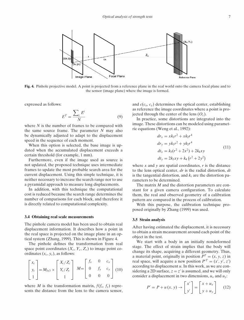
Fig. 4. Pinhole projective model. A point is projected from a reference plane in the real world onto the camera focal plane and tothe sensor (image plane) where the image is formed.

expressed as follows:

ET =∑

iEi

N(9)

where N is the number of frames to be compared withthe same source frame. The parameter N may alsobe dynamically adjusted to adapt to the displacementspeed in the sequence of each moment.

When this option is selected, the base image is up-dated when the accumulated displacement exceeds acertain threshold (for example, 1 mm).

Furthermore, even if the image used as source isnot updated, the proposed technique uses intermediateframes to update the most probable search area for thecurrent displacement. Using this simple technique, it isneither necessary to increase the search range nor to usea pyramidal approach to measure long displacements.

In addition, with this technique the computationalcost is reduced because the search range determines thenumber of comparisons for each block, and therefore itis directly related to computational complexity.

3.4 Obtaining real scale measurements

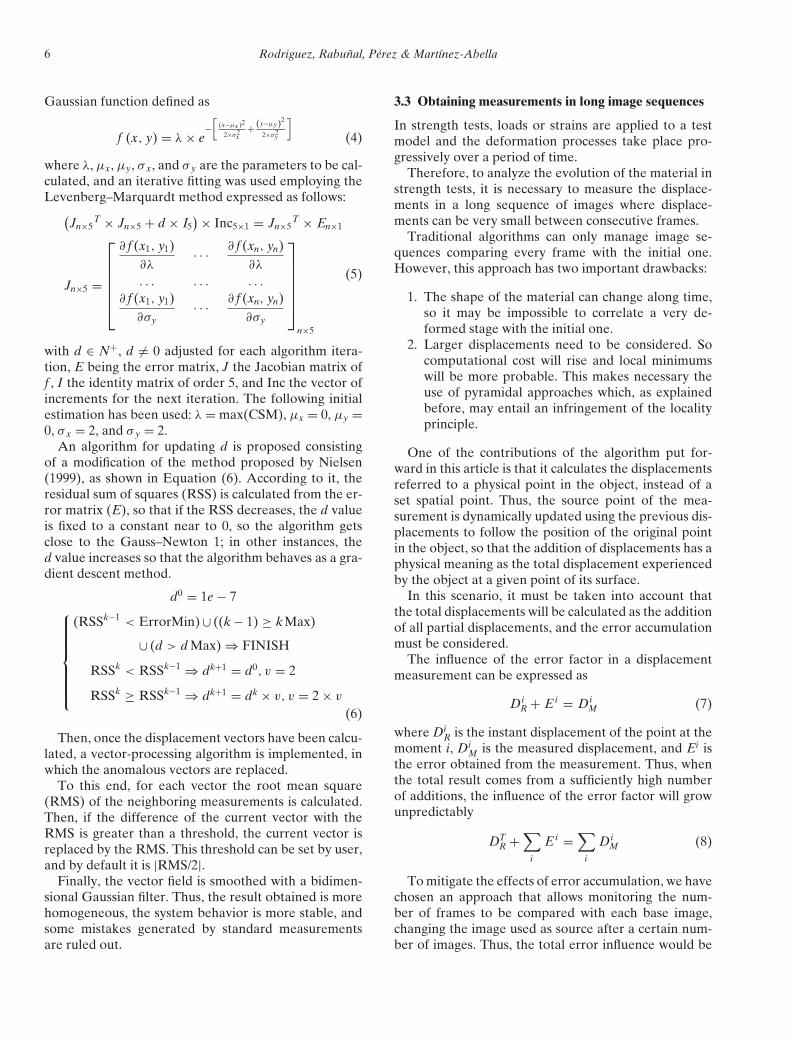
The pinhole camera model has been used to obtain realdisplacement information. It describes how a point inthe real space is projected on the image plane in an op-tical system (Zhang, 1999). This is shown in Figure 4.

The pinhole defines the transformation from realspace point coordinates (Xc, Yc, Zc) to image point co-ordinates (xc, yc), as follows:⎡

⎢⎢⎣xc

yc

1

⎤⎥⎥⎦=M3x3 ×

⎡⎢⎢⎣

Xc/Zc

Yc/Zc

1

⎤⎥⎥⎦ M=

⎡⎢⎢⎣

fx 0 cx

0 fy cy

0 0 0

⎤⎥⎥⎦ (10)

where M is the transformation matrix, f (fx, fy) repre-sents the distance from the lens to the camera sensor,

and c(cx, cy) determines the optical center, establishingas reference the image coordinates where a point is pro-jected through the center of the lens (Oc).

In practice, some distortions are integrated into theimage. These distortions can be modeled using paramet-ric equations (Weng et al., 1992):

drx = xk1r2 + xk2r4

dry = yk1r2 + yk2r4

dtx = k3(r2 + 2x2) + 2k4xy

dty = 2k3xy + k4(r2 + 2y2

)(11)

where x and y are spatial coordinates, r is the distanceto the lens optical center, dr is the radial distortion, dtis the tangential distortion, and ki are the distortion pa-rameters to be determined.

The matrix M and the distortion parameters are con-stant for a given camera configuration. To calculatethem, the real and observed geometry of a calibrationpattern are compared in the process of calibration.

With this purpose, the calibration technique pro-posed originally by Zhang (1999) was used.

3.5 Strain analysis

After having estimated the displacement, it is necessaryto obtain a strain measurement around each point of theobject in the test.

We start with a body in an initially nondeformedstage. The effect of strain implies that the body willchange its shape, acquiring a different geometry. Thus,a material point, originally in position PT = (x, y, z) inreal space, will acquire a new position P′T = (x′, y′, z′)according to displacement u. In this work, as we are con-sidering a 2D surface, z = z′ is assumed, and we will onlyconsider a displacement in two dimensions, ux and uy:

P′ = P + u (x, y) →[

x′

y′

]=

[x + ux

y + uy

](12)


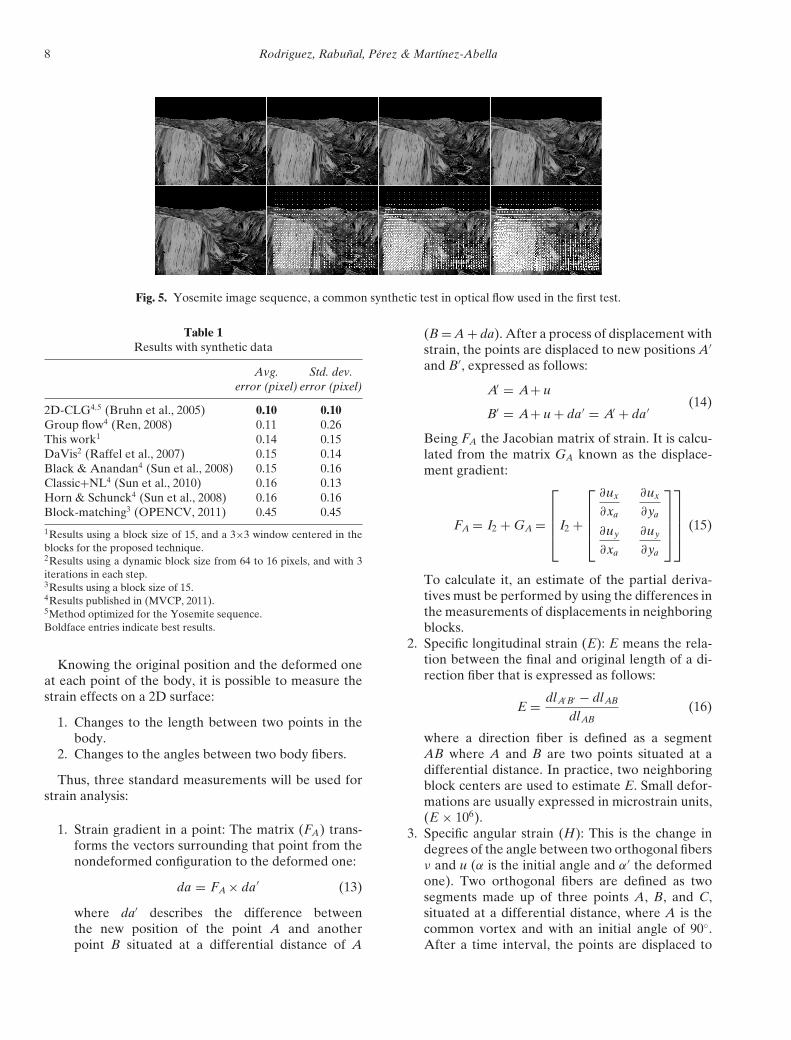
Fig. 5. Yosemite image sequence, a common synthetic test in optical flow used in the first test.

Table 1Results with synthetic data

Avg. Std. dev.error (pixel) error (pixel)

2D-CLG4,5 (Bruhn et al., 2005) 0.10 0.10Group flow4 (Ren, 2008) 0.11 0.26This work1 0.14 0.15DaVis2 (Raffel et al., 2007) 0.15 0.14Black & Anandan4 (Sun et al., 2008) 0.15 0.16Classic+NL4 (Sun et al., 2010) 0.16 0.13Horn & Schunck4 (Sun et al., 2008) 0.16 0.16Block-matching3 (OPENCV, 2011) 0.45 0.45

1Results using a block size of 15, and a 3×3 window centered in theblocks for the proposed technique.2Results using a dynamic block size from 64 to 16 pixels, and with 3iterations in each step.3Results using a block size of 15.4Results published in (MVCP, 2011).5Method optimized for the Yosemite sequence.Boldface entries indicate best results.

Knowing the original position and the deformed oneat each point of the body, it is possible to measure thestrain effects on a 2D surface:

1. Changes to the length between two points in thebody.

2. Changes to the angles between two body fibers.

Thus, three standard measurements will be used forstrain analysis:

1. Strain gradient in a point: The matrix (FA) trans-forms the vectors surrounding that point from thenondeformed configuration to the deformed one:

da = FA × da′ (13)

where da′ describes the difference betweenthe new position of the point A and anotherpoint B situated at a differential distance of A

(B = A + da). After a process of displacement withstrain, the points are displaced to new positions A′

and B′, expressed as follows:

A′ = A+ u

B′ = A+ u + da′ = A′ + da′ (14)

Being FA the Jacobian matrix of strain. It is calcu-lated from the matrix GA known as the displace-ment gradient:

FA = I2 + GA =

⎡⎢⎢⎢⎣I2 +

⎡⎢⎢⎢⎣

∂ux

∂xa

∂ux

∂ya

∂uy

∂xa

∂uy

∂ya

⎤⎥⎥⎥⎦

⎤⎥⎥⎥⎦ (15)

To calculate it, an estimate of the partial deriva-tives must be performed by using the differences inthe measurements of displacements in neighboringblocks.

2. Specific longitudinal strain (E): E means the rela-tion between the final and original length of a di-rection fiber that is expressed as follows:

E = dlA′ B′ − dlAB

dlAB(16)

where a direction fiber is defined as a segmentAB where A and B are two points situated at adifferential distance. In practice, two neighboringblock centers are used to estimate E. Small defor-mations are usually expressed in microstrain units,(E × 106).

3. Specific angular strain (H): This is the change indegrees of the angle between two orthogonal fibersν and u (α is the initial angle and α′ the deformedone). Two orthogonal fibers are defined as twosegments made up of three points A, B, and C,situated at a differential distance, where A is thecommon vortex and with an initial angle of 90◦.After a time interval, the points are displaced to


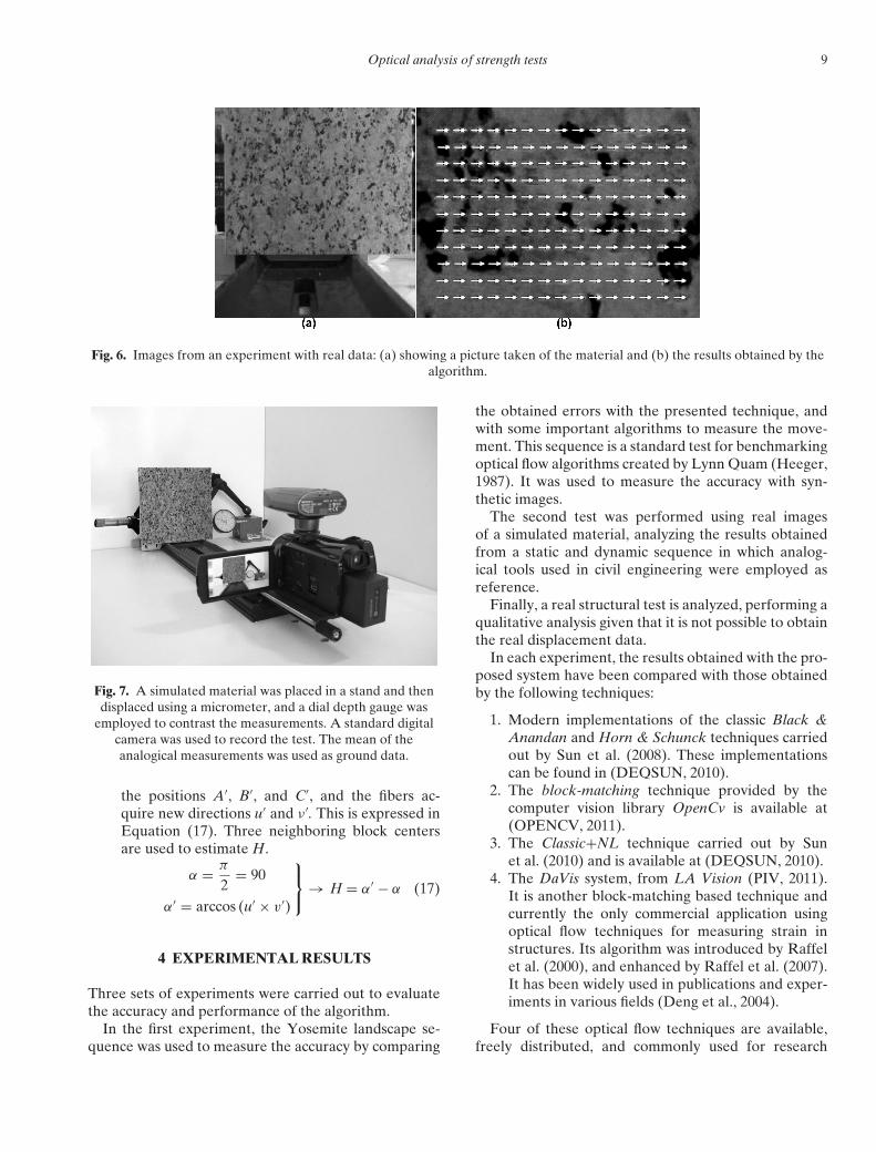
Fig. 6. Images from an experiment with real data: (a) showing a picture taken of the material and (b) the results obtained by thealgorithm.

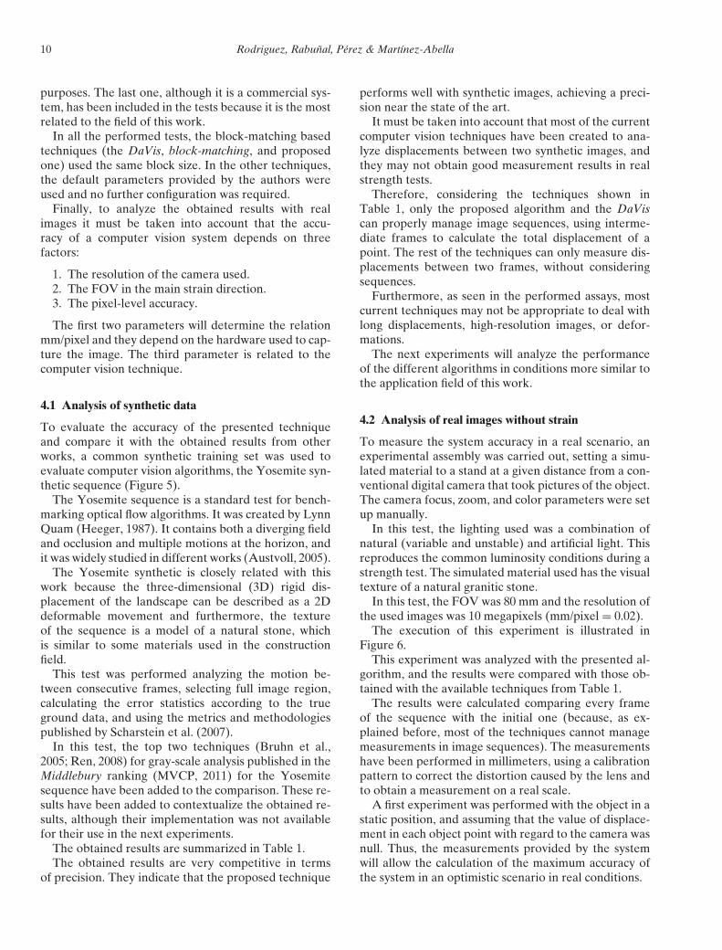
Fig. 7. A simulated material was placed in a stand and thendisplaced using a micrometer, and a dial depth gauge was

employed to contrast the measurements. A standard digitalcamera was used to record the test. The mean of theanalogical measurements was used as ground data.

the positions A′, B′, and C′, and the fibers ac-quire new directions u′ and ν ′. This is expressed inEquation (17). Three neighboring block centersare used to estimate H.

α = π

2= 90

α′ = arccos (u′ × v′)

⎫⎬⎭ → H = α′ − α (17)

4 EXPERIMENTAL RESULTS

Three sets of experiments were carried out to evaluatethe accuracy and performance of the algorithm.

In the first experiment, the Yosemite landscape se-quence was used to measure the accuracy by comparing

the obtained errors with the presented technique, andwith some important algorithms to measure the move-ment. This sequence is a standard test for benchmarkingoptical flow algorithms created by Lynn Quam (Heeger,1987). It was used to measure the accuracy with syn-thetic images.

The second test was performed using real imagesof a simulated material, analyzing the results obtainedfrom a static and dynamic sequence in which analog-ical tools used in civil engineering were employed asreference.

Finally, a real structural test is analyzed, performing aqualitative analysis given that it is not possible to obtainthe real displacement data.

In each experiment, the results obtained with the pro-posed system have been compared with those obtainedby the following techniques:

1. Modern implementations of the classic Black &Anandan and Horn & Schunck techniques carriedout by Sun et al. (2008). These implementationscan be found in (DEQSUN, 2010).

2. The block-matching technique provided by thecomputer vision library OpenCv is available at(OPENCV, 2011).

3. The Classic+NL technique carried out by Sunet al. (2010) and is available at (DEQSUN, 2010).

4. The DaVis system, from LA Vision (PIV, 2011).It is another block-matching based technique andcurrently the only commercial application usingoptical flow techniques for measuring strain instructures. Its algorithm was introduced by Raffelet al. (2000), and enhanced by Raffel et al. (2007).It has been widely used in publications and exper-iments in various fields (Deng et al., 2004).

Four of these optical flow techniques are available,freely distributed, and commonly used for research


purposes. The last one, although it is a commercial sys-tem, has been included in the tests because it is the mostrelated to the field of this work.

In all the performed tests, the block-matching basedtechniques (the DaVis, block-matching, and proposedone) used the same block size. In the other techniques,the default parameters provided by the authors wereused and no further configuration was required.

Finally, to analyze the obtained results with realimages it must be taken into account that the accu-racy of a computer vision system depends on threefactors:

1. The resolution of the camera used.2. The FOV in the main strain direction.3. The pixel-level accuracy.

The first two parameters will determine the relationmm/pixel and they depend on the hardware used to cap-ture the image. The third parameter is related to thecomputer vision technique.

4.1 Analysis of synthetic data

To evaluate the accuracy of the presented techniqueand compare it with the obtained results from otherworks, a common synthetic training set was used toevaluate computer vision algorithms, the Yosemite syn-thetic sequence (Figure 5).

The Yosemite sequence is a standard test for bench-marking optical flow algorithms. It was created by LynnQuam (Heeger, 1987). It contains both a diverging fieldand occlusion and multiple motions at the horizon, andit was widely studied in different works (Austvoll, 2005).

The Yosemite synthetic is closely related with thiswork because the three-dimensional (3D) rigid dis-placement of the landscape can be described as a 2Ddeformable movement and furthermore, the textureof the sequence is a model of a natural stone, whichis similar to some materials used in the constructionfield.

This test was performed analyzing the motion be-tween consecutive frames, selecting full image region,calculating the error statistics according to the trueground data, and using the metrics and methodologiespublished by Scharstein et al. (2007).

In this test, the top two techniques (Bruhn et al.,2005; Ren, 2008) for gray-scale analysis published in theMiddlebury ranking (MVCP, 2011) for the Yosemitesequence have been added to the comparison. These re-sults have been added to contextualize the obtained re-sults, although their implementation was not availablefor their use in the next experiments.

The obtained results are summarized in Table 1.The obtained results are very competitive in terms

of precision. They indicate that the proposed technique

performs well with synthetic images, achieving a preci-sion near the state of the art.

It must be taken into account that most of the currentcomputer vision techniques have been created to ana-lyze displacements between two synthetic images, andthey may not obtain good measurement results in realstrength tests.

Therefore, considering the techniques shown inTable 1, only the proposed algorithm and the DaViscan properly manage image sequences, using interme-diate frames to calculate the total displacement of apoint. The rest of the techniques can only measure dis-placements between two frames, without consideringsequences.

Furthermore, as seen in the performed assays, mostcurrent techniques may not be appropriate to deal withlong displacements, high-resolution images, or defor-mations.

The next experiments will analyze the performanceof the different algorithms in conditions more similar tothe application field of this work.

4.2 Analysis of real images without strain

To measure the system accuracy in a real scenario, anexperimental assembly was carried out, setting a simu-lated material to a stand at a given distance from a con-ventional digital camera that took pictures of the object.The camera focus, zoom, and color parameters were setup manually.

In this test, the lighting used was a combination ofnatural (variable and unstable) and artificial light. Thisreproduces the common luminosity conditions during astrength test. The simulated material used has the visualtexture of a natural granitic stone.

In this test, the FOV was 80 mm and the resolution ofthe used images was 10 megapixels (mm/pixel = 0.02).

The execution of this experiment is illustrated inFigure 6.

This experiment was analyzed with the presented al-gorithm, and the results were compared with those ob-tained with the available techniques from Table 1.

The results were calculated comparing every frameof the sequence with the initial one (because, as ex-plained before, most of the techniques cannot managemeasurements in image sequences). The measurementshave been performed in millimeters, using a calibrationpattern to correct the distortion caused by the lens andto obtain a measurement on a real scale.

A first experiment was performed with the object in astatic position, and assuming that the value of displace-ment in each object point with regard to the camera wasnull. Thus, the measurements provided by the systemwill allow the calculation of the maximum accuracy ofthe system in an optimistic scenario in real conditions.


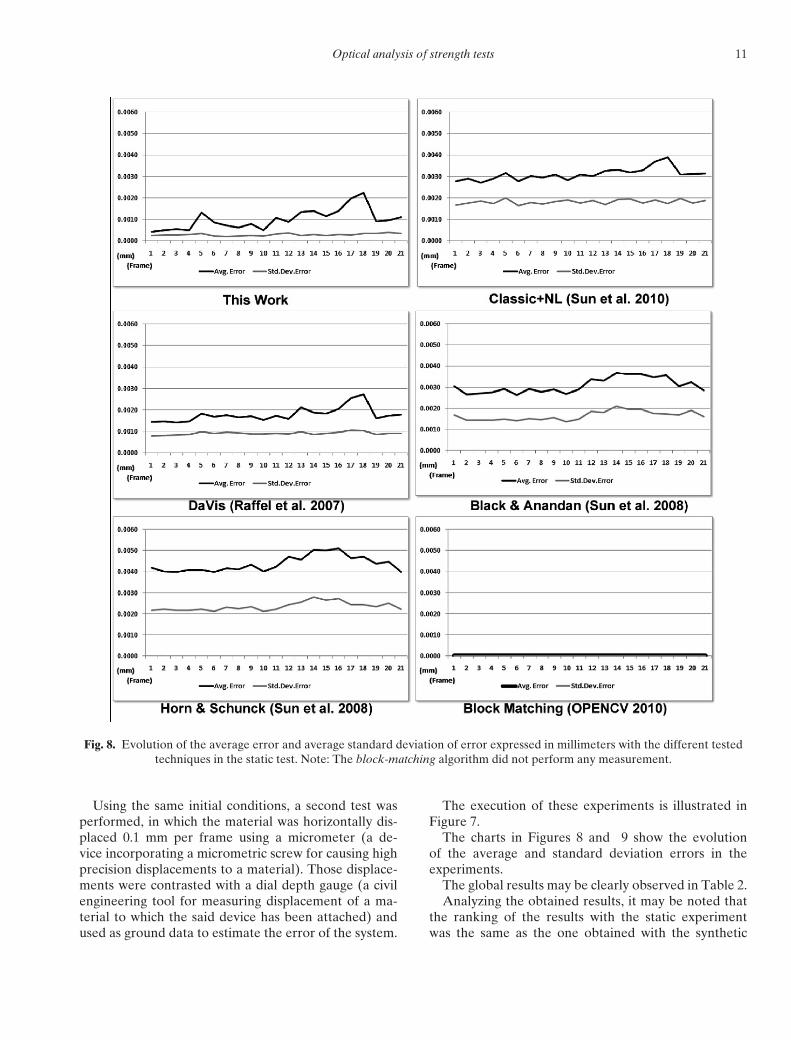
Fig. 8. Evolution of the average error and average standard deviation of error expressed in millimeters with the different testedtechniques in the static test. Note: The block-matching algorithm did not perform any measurement.

Using the same initial conditions, a second test wasperformed, in which the material was horizontally dis-placed 0.1 mm per frame using a micrometer (a de-vice incorporating a micrometric screw for causing highprecision displacements to a material). Those displace-ments were contrasted with a dial depth gauge (a civilengineering tool for measuring displacement of a ma-terial to which the said device has been attached) andused as ground data to estimate the error of the system.

The execution of these experiments is illustrated inFigure 7.

The charts in Figures 8 and 9 show the evolutionof the average and standard deviation errors in theexperiments.

The global results may be clearly observed in Table 2.Analyzing the obtained results, it may be noted that

the ranking of the results with the static experimentwas the same as the one obtained with the synthetic


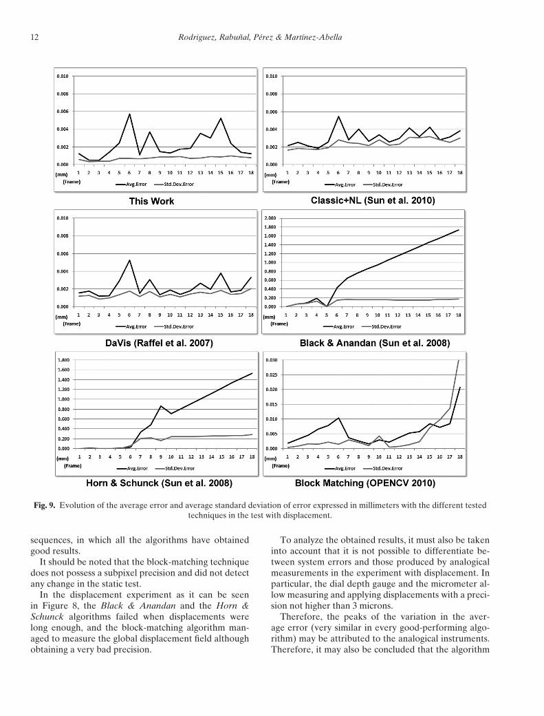
Fig. 9. Evolution of the average error and average standard deviation of error expressed in millimeters with the different testedtechniques in the test with displacement.

sequences, in which all the algorithms have obtainedgood results.

It should be noted that the block-matching techniquedoes not possess a subpixel precision and did not detectany change in the static test.

In the displacement experiment as it can be seenin Figure 8, the Black & Anandan and the Horn &Schunck algorithms failed when displacements werelong enough, and the block-matching algorithm man-aged to measure the global displacement field althoughobtaining a very bad precision.

To analyze the obtained results, it must also be takeninto account that it is not possible to differentiate be-tween system errors and those produced by analogicalmeasurements in the experiment with displacement. Inparticular, the dial depth gauge and the micrometer al-low measuring and applying displacements with a preci-sion not higher than 3 microns.

Therefore, the peaks of the variation in the aver-age error (very similar in every good-performing algo-rithm) may be attributed to the analogical instruments.Therefore, it may also be concluded that the algorithm


Table 2Results of experiments with real images of a simulated

material

Static Displacementexperiment experiment

Global Global Global Globalavg. std. dev. avg. std. dev.error error error error(mm) (mm) (mm) (mm)

This work 0.0010 0.0003 0.0022 0.0007DaVis (Raffel

et al., 2007)0.0018 0.0009 0.0022 0.0014

Classic+NL(Sun et al.,2010)

0.0031 0.0018 0.0032 0.0024

Block-matching(OPENCV,2011)

0.00001 0.00001 0.0059 0.0048

Black &Anandan(Sun et al.,2008)

0.0031 0.0017 0.8421 0.130

Horn &Schunck(Sun et al.,2008)

0.0048 0.0024 0.6579 0.1644

1The block-matching algorithm did not perform any measurement inthe static experiment.

presented, together with the DaVis and Classic+NLones, was significantly more accurate and stable than theanalogical tools used as reference.

The best results in this experiment have been ob-tained by the DaVis system and the proposed technique.

It may be concluded that the proposed technique canobtain very accurate results with real images. In addi-tion, the measurements obtained in the performed testswere similar in accuracy and better in stability than theanalogical tools used as reference.

Furthermore, the accuracy in the proposed system islinked to the pixel level, so, theoretically it is limitedonly by the zoom and resolution of the camera used.

4.3 Analysis of real strength tests

Different tests in a scenario with real strains have beenperformed to analyze the algorithm behavior in the ap-plication field of this work.

The goal will be to determine the validity and poten-tial application of the algorithm in a real scenario. Forthis purpose, three strength tests have been carried outwith different materials and forces.

1. In the first tests, a steel bar under tensile forces wasstudied. In this test, the obtained results were com-

pared with those obtained by the computer visiontechniques used in the previous tests.

2. In the second test a concrete test model undercompression forces was analyzed. In this test, theproposed technique was compared with data ob-tained with standard strain gauges.

3. In the last experiment, an aluminum bar un-der tensile forces was tested. Obtained resultswere compared with those provided by a contactextensometer.

These tests were carried out at the Centre of Techno-logical Innovation in Construction and Civil Engineer-ing (CITEEC) and they are standard tests in the civilengineering field.

The materials are painted with a random spot distri-bution to provide a visual texture.

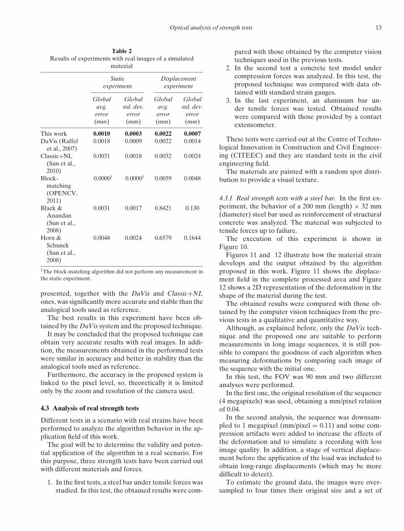
4.3.1 Real strength tests with a steel bar. In the first ex-periment, the behavior of a 200 mm (length) × 32 mm(diameter) steel bar used as reinforcement of structuralconcrete was analyzed. The material was subjected totensile forces up to failure.

The execution of this experiment is shown inFigure 10.

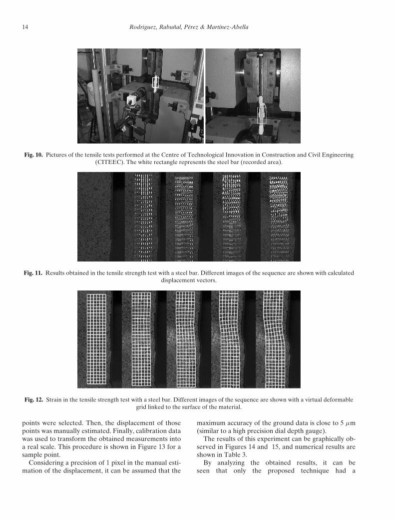
Figures 11 and 12 illustrate how the material straindevelops and the output obtained by the algorithmproposed in this work. Figure 11 shows the displace-ment field in the complete processed area and Figure12 shows a 2D representation of the deformation in theshape of the material during the test.

The obtained results were compared with those ob-tained by the computer vision techniques from the pre-vious tests in a qualitative and quantitative way.

Although, as explained before, only the DaVis tech-nique and the proposed one are suitable to performmeasurements in long image sequences, it is still pos-sible to compare the goodness of each algorithm whenmeasuring deformations by comparing each image ofthe sequence with the initial one.

In this test, the FOV was 90 mm and two differentanalyses were performed.

In the first one, the original resolution of the sequence(4 megapixels) was used, obtaining a mm/pixel relationof 0.04.

In the second analysis, the sequence was downsam-pled to 1 megapixel (mm/pixel = 0.11) and some com-pression artifacts were added to increase the effects ofthe deformation and to simulate a recording with lessimage quality. In addition, a stage of vertical displace-ment before the application of the load was included toobtain long-range displacements (which may be moredifficult to detect).

To estimate the ground data, the images were over-sampled to four times their original size and a set of


Fig. 10. Pictures of the tensile tests performed at the Centre of Technological Innovation in Construction and Civil Engineering(CITEEC). The white rectangle represents the steel bar (recorded area).

Fig. 11. Results obtained in the tensile strength test with a steel bar. Different images of the sequence are shown with calculateddisplacement vectors.

Fig. 12. Strain in the tensile strength test with a steel bar. Different images of the sequence are shown with a virtual deformablegrid linked to the surface of the material.

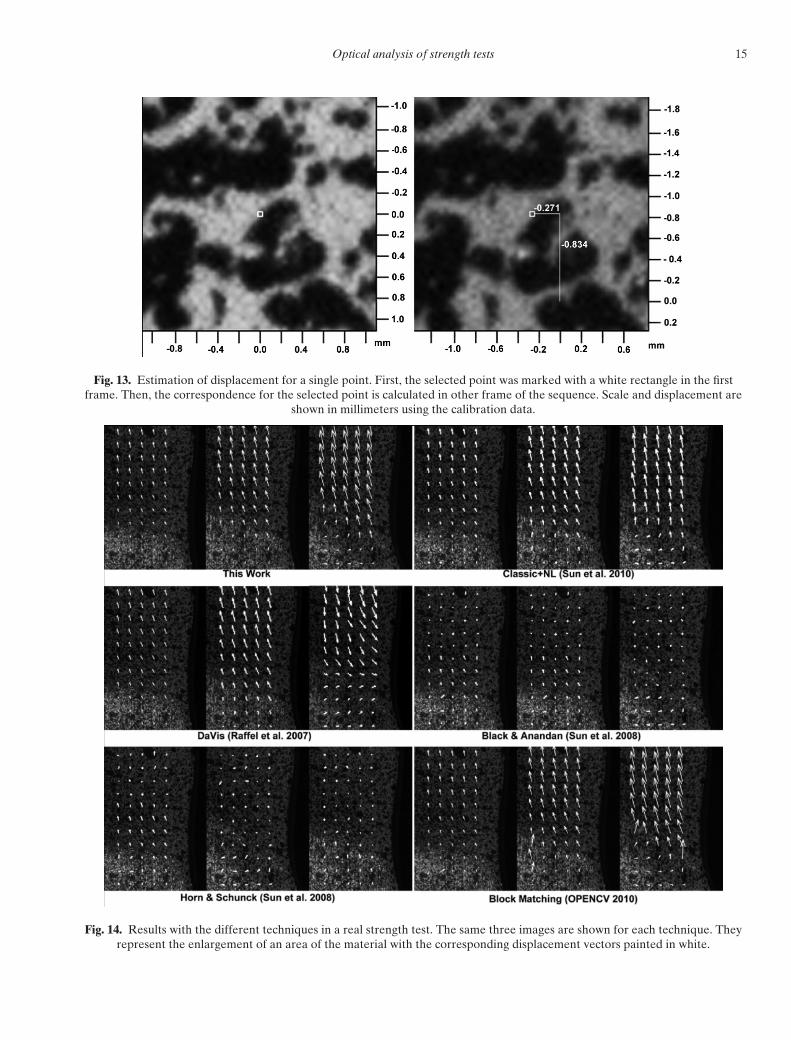
points were selected. Then, the displacement of thosepoints was manually estimated. Finally, calibration datawas used to transform the obtained measurements intoa real scale. This procedure is shown in Figure 13 for asample point.

Considering a precision of 1 pixel in the manual esti-mation of the displacement, it can be assumed that the

maximum accuracy of the ground data is close to 5 μm(similar to a high precision dial depth gauge).

The results of this experiment can be graphically ob-served in Figures 14 and 15, and numerical results areshown in Table 3.

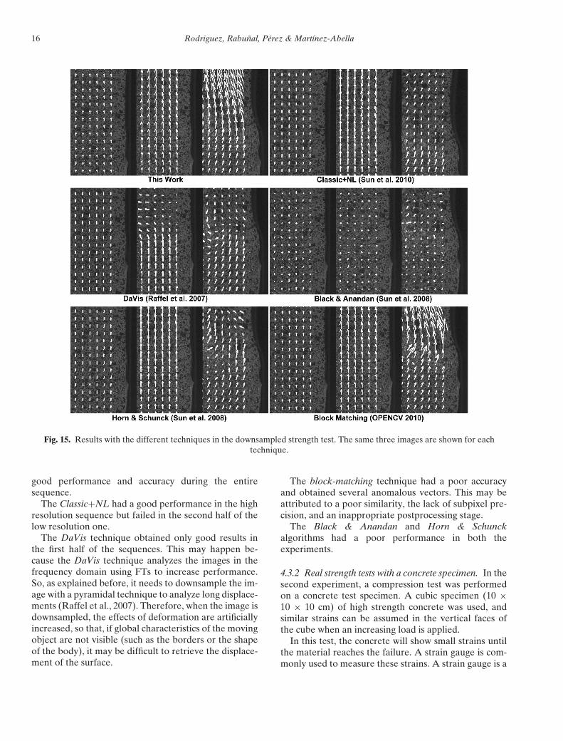
By analyzing the obtained results, it can beseen that only the proposed technique had a


Fig. 13. Estimation of displacement for a single point. First, the selected point was marked with a white rectangle in the firstframe. Then, the correspondence for the selected point is calculated in other frame of the sequence. Scale and displacement are

shown in millimeters using the calibration data.

Fig. 14. Results with the different techniques in a real strength test. The same three images are shown for each technique. Theyrepresent the enlargement of an area of the material with the corresponding displacement vectors painted in white.


Fig. 15. Results with the different techniques in the downsampled strength test. The same three images are shown for eachtechnique.

good performance and accuracy during the entiresequence.

The Classic+NL had a good performance in the highresolution sequence but failed in the second half of thelow resolution one.

The DaVis technique obtained only good results inthe first half of the sequences. This may happen be-cause the DaVis technique analyzes the images in thefrequency domain using FTs to increase performance.So, as explained before, it needs to downsample the im-age with a pyramidal technique to analyze long displace-ments (Raffel et al., 2007). Therefore, when the image isdownsampled, the effects of deformation are artificiallyincreased, so that, if global characteristics of the movingobject are not visible (such as the borders or the shapeof the body), it may be difficult to retrieve the displace-ment of the surface.

The block-matching technique had a poor accuracyand obtained several anomalous vectors. This may beattributed to a poor similarity, the lack of subpixel pre-cision, and an inappropriate postprocessing stage.

The Black & Anandan and Horn & Schunckalgorithms had a poor performance in both theexperiments.

4.3.2 Real strength tests with a concrete specimen. In thesecond experiment, a compression test was performedon a concrete test specimen. A cubic specimen (10 ×10 × 10 cm) of high strength concrete was used, andsimilar strains can be assumed in the vertical faces ofthe cube when an increasing load is applied.

In this test, the concrete will show small strains untilthe material reaches the failure. A strain gauge is com-monly used to measure these strains. A strain gauge is a


Table 3Numerical results of the tensile test with a steel bar

High resolutionexperiment

Low resolutionexperiment

Avg. Std. dev. Avg. Std. dev.error error error error(mm) (mm) (mm) (mm)

This work 0.008 0.004 0.031 0.028Block-

matching(OPENCV,2011)

0.046 0.036 0.171 0.326

Classic+NL(Sun et al.,2010)

0.062 0.022 1.140 2.149

Horn &Schunck(Sun et al.,2008)

1.507 1.195 1.065 1.958

DaVis (Raffelet al., 2007)

1.318 2.049 1.937 2.389

Black &Anandan(Sun et al.,2008)

1.551 1.180 2.091 1.947

device that uses electrical conductance to measure smallstrains with high accuracy.

Strain gauges need to be attached to the mate-rial before the test, provide measurements in a sin-gle direction, and they fail when the material breaks.

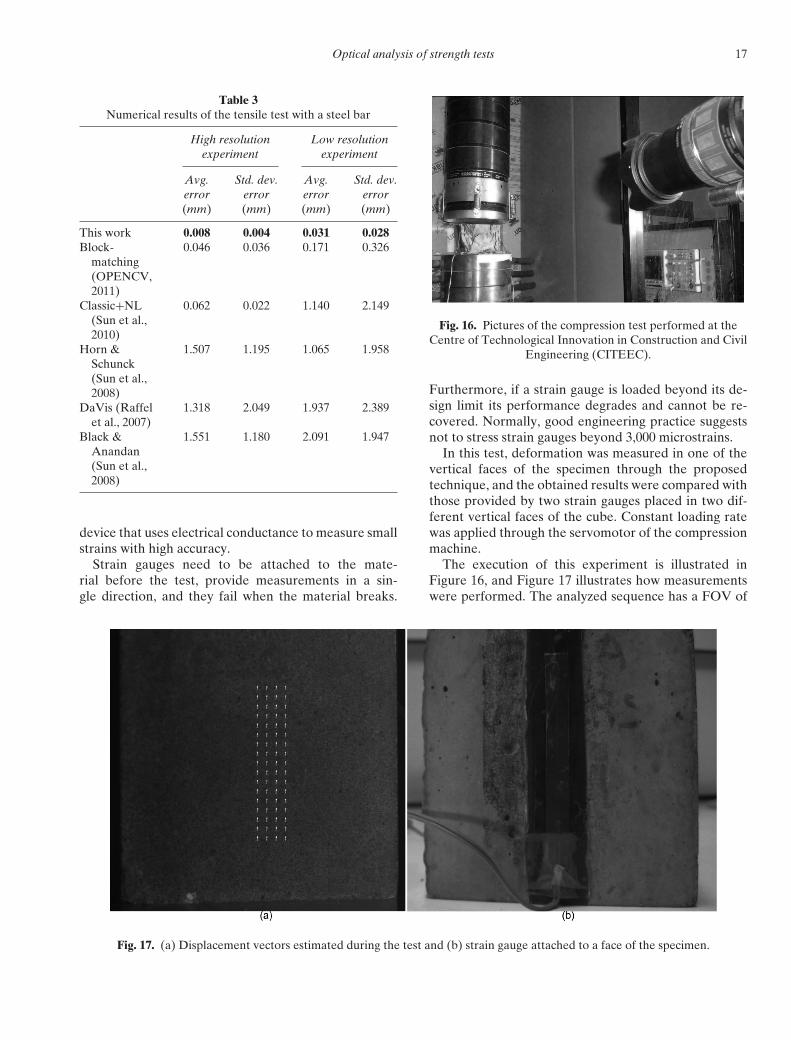
Fig. 16. Pictures of the compression test performed at theCentre of Technological Innovation in Construction and Civil

Engineering (CITEEC).

Furthermore, if a strain gauge is loaded beyond its de-sign limit its performance degrades and cannot be re-covered. Normally, good engineering practice suggestsnot to stress strain gauges beyond 3,000 microstrains.

In this test, deformation was measured in one of thevertical faces of the specimen through the proposedtechnique, and the obtained results were compared withthose provided by two strain gauges placed in two dif-ferent vertical faces of the cube. Constant loading ratewas applied through the servomotor of the compressionmachine.

The execution of this experiment is illustrated inFigure 16, and Figure 17 illustrates how measurementswere performed. The analyzed sequence has a FOV of

Fig. 17. (a) Displacement vectors estimated during the test and (b) strain gauge attached to a face of the specimen.


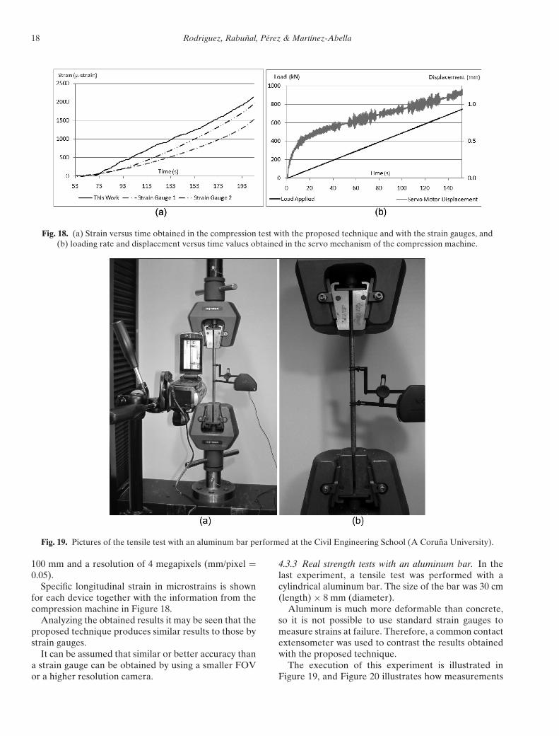
Fig. 18. (a) Strain versus time obtained in the compression test with the proposed technique and with the strain gauges, and(b) loading rate and displacement versus time values obtained in the servo mechanism of the compression machine.

Fig. 19. Pictures of the tensile test with an aluminum bar performed at the Civil Engineering School (A Coruna University).

100 mm and a resolution of 4 megapixels (mm/pixel =0.05).

Specific longitudinal strain in microstrains is shownfor each device together with the information from thecompression machine in Figure 18.

Analyzing the obtained results it may be seen that theproposed technique produces similar results to those bystrain gauges.

It can be assumed that similar or better accuracy thana strain gauge can be obtained by using a smaller FOVor a higher resolution camera.

4.3.3 Real strength tests with an aluminum bar. In thelast experiment, a tensile test was performed with acylindrical aluminum bar. The size of the bar was 30 cm(length) × 8 mm (diameter).

Aluminum is much more deformable than concrete,so it is not possible to use standard strain gauges tomeasure strains at failure. Therefore, a common contactextensometer was used to contrast the results obtainedwith the proposed technique.

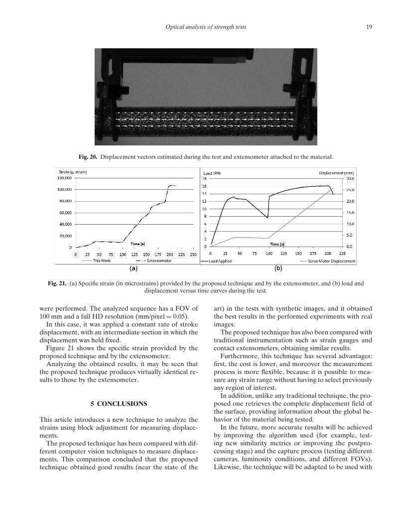
The execution of this experiment is illustrated inFigure 19, and Figure 20 illustrates how measurements


Fig. 20. Displacement vectors estimated during the test and extensometer attached to the material.

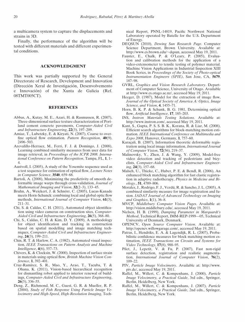
Fig. 21. (a) Specific strain (in microstrains) provided by the proposed technique and by the extensometer, and (b) load anddisplacement versus time curves during the test.

were performed. The analyzed sequence has a FOV of100 mm and a full HD resolution (mm/pixel = 0.05).

In this case, it was applied a constant rate of strokedisplacement, with an intermediate section in which thedisplacement was held fixed.

Figure 21 shows the specific strain provided by theproposed technique and by the extensometer.

Analyzing the obtained results, it may be seen thatthe proposed technique produces virtually identical re-sults to those by the extensometer.

5 CONCLUSIONS

This article introduces a new technique to analyze thestrains using block adjustment for measuring displace-ments.

The proposed technique has been compared with dif-ferent computer vision techniques to measure displace-ments. This comparison concluded that the proposedtechnique obtained good results (near the state of the

art) in the tests with synthetic images, and it obtainedthe best results in the performed experiments with realimages.

The proposed technique has also been compared withtraditional instrumentation such as strain gauges andcontact extensometers, obtaining similar results.

Furthermore, this technique has several advantages:first, the cost is lower, and moreover the measurementprocess is more flexible, because it is possible to mea-sure any strain range without having to select previouslyany region of interest.

In addition, unlike any traditional technique, the pro-posed one retrieves the complete displacement field ofthe surface, providing information about the global be-havior of the material being tested.

In the future, more accurate results will be achievedby improving the algorithm used (for example, test-ing new similarity metrics or improving the postpro-cessing stage) and the capture process (testing differentcameras, luminosity conditions, and different FOVs).Likewise, the technique will be adapted to be used with


a multicamera system to capture the displacements andstrains in 3D.

Finally, the performance of the algorithm will betested with different materials and different experimen-tal conditions.

ACKNOWLEDGMENT

This work was partially supported by the GeneralDirectorate of Research, Development and Innovation(Direccion Xeral de Investigacion, Desenvolvementoe Innovacion) of the Xunta de Galicia (Ref.08TMT005CT).

REFERENCES

Abbas, A., Kutay, M. E., Azari, H. & Rasmussen, R. (2007),Three-dimensional surface texture characterization of Port-land cement concrete pavements, Computer-Aided Civiland Infrastructure Engineering, 22(3), 197–209.

Amiaz, T., Lubetzky, E. & Kiryati, N. (2007), Coarse to over-fine optical flow estimation. Pattern Recognition, 40(9),2496–503.

Arevalillo-Herraez, M., Ferri, F. J. & Domingo, J. (2008),Learning combined similarity measures from user data forimage retrieval, in Proceedings of the ICPR 2008. Interna-tional Conference on Pattern Recognition, Tampa, FL, 1, 1–4.

Austvoll, I. (2005), A study of the Yosemite sequence used asa test sequence for estimation of optical flow, Lecture Notesin Computer Science, 3540, 659–68.

Bartoli, A. (2008), Maximizing the predictivity of smooth de-formable image warps through cross-validation, Journal ofMathematical Imaging and Vision, 32(2–3), 133–45.

Bruhn, A., Weickert, J. & Schnorr, C. (2005), Lucas-Kanademeets Horn-Schunck: combining local and global optic flowmethods, International Journal of Computer Vision, 61(3),211–31.

Chi, S. & Caldas, C. H. (2011), Automated object identifica-tion using video cameras on construction sites, Computer-Aided Civil and Infrastructure Engineering, 26(5), 368–80.

Chi, S., Caldas, C. H. & Kim, D. Y. (2009), A methodologyfor object identification and tracking in constructionbased on spatial modelling and image matching tech-niques, Computer-Aided Civil and Infrastructure Engineer-ing, 24(3), 199–211.

Chin, R. T. & Harlow, C. A. (1982), Automated visual inspec-tion, IEEE Transactions on Pattern Analysis and MachineIntelligence, 4(6), 557–73.

Chivers, K. & Clocksin, W. (2000), Inspection of surface strainin materials using optical flow, British Machine Vision Con-ference, 1, 392–401.

Cruz-Ramırez, S. R., Mao, Y., Arao, T., Tacuba, T. &Ohana, K. (2011), Vision-based hierarchical recognitionfor dismantling robot applied to interior renewal of build-ings, Computer-Aided Civil and Infrastructure Engineering,26(5), 336–55.

Deng, Z., Richmond, M. C., Guest, G. R. & Mueller, R. P.(2004), Study of Fish Response Using Particle Image Ve-locimetry and High-Speed, High-Resolution Imaging, Tech-

nical Report, PNNL-14819, Pacific Northwest NationalLaboratory operated by Batelle for the U.S. Departmentof Energy.

DEQSUN (2010), Dewing Sun Research Page. ComputerScience Department, Brown University. Available at:http://www.cs.brown.edu/∼dqsun, accessed May 19, 2011.

Fauster, E., Chalk, P. & O’Leary, P. (2005), Evalua-tion and calibration methods for the application of avideo-extensometer to tensile testing of polymer material.Machine Vision Applications in Industrial Inspection XIIIBook Series, in Proceedings of the Society of Photo-opticalInstrumentation Engineers (SPIE), San Jose, CA, 5679,187–98.

GVRL, Graphics and Vision Research Laboratory. Depart-ment of Computer Science, University of Otago. Availableat http://www.cs.otago.ac.nz/, accessed May 19, 2011.

Heeger, D. (1987), Model for the extraction of image flow,Journal of the Optical Society of America A: Optics, ImageScience, and Vision, 4, 1455–71.

Horn, B. K. P. & Schunk, B. G. 1981, Determining opticalflow, Artificial Intelligence, 17, 185–203.

INS, Instron Materials Testing Solutions. Available at:http://www.instron.com/, accessed May 19, 2011.

Kant, S., Gupta, P. S. S. B. K., Korana, R. & Liar, M. (2008),Efficient search algorithms for block-matching motion esti-mation. IEEE International Conference on Multimedia andExpo 2008, Hanover, Germany, 1, 757–60.

Karacali, B. (2007), Information theoretic deformable regis-tration using local image information, International Journalof Computer Vision, 72(56), 219–37.

Malinovsky, Y., Zhen, J. & Wang, Y. (2009), Model-freevideo detection and tracking of pedestrians and bicy-clists, Computer-Aided Civil and Infrastructure Engineer-ing, 24(3), 157–68.

Malsch, U., Thieke, C., Huber, P. E. & Bendl, R. (2006), Anenhanced block matching algorithm for fast elastic registra-tion in adaptive radiotherapy, Physics in Medicine and Bi-ology., 51, 4789–806.

Morales, J., Rodrigo, F. J., Verdu, R. & Sancho, J. L. (2005), Acombined similarity measure for image registration and fu-sion. IADAT Journal of Advanced Technology on Imagingand Graphics, 1(1), 36–8.

MVCP, Middlebury Computer Vision Pages. Available at:http://vision.middlebury.edu/, accessed May 19, 2011.

Nielsen, H. B. (1999), Damping Parameter in Marquardt’sMethod, Technical Report, IMM-REP-1999—05, TechnicalUniversity of Denmark, Denmark.

OPENCV, Open Source Computer Vision. Available at:http://opencv.willowgarage.com/, accessed May 19, 2011.

Patras, I., Hendriks, E. A. & Lagendijk, R. L. (2007), Proba-bilistic confidence measures for block matching motion es-timation, IEEE Transactions on Circuits and Systems forVideo Technology, 17(8), 988–95.

Pilet, J., Lepetit, V. & Fu, P. (2007), Fast non-rigidsurface detection, registration and realistic augmenta-tion, International Journal of Computer Vision, 76(2),109–22.

PIV, Particle Image Velocimetry. Available at: http://www.piv.de/, accessed May 19, 2011.

Raffel, M., Willert, C. & Kompenhans, J. (2000), ParticleImage Velocimetry, a Practical Guide, 3rd edn., Springer,Berlin, Heidelberg, New York.

Raffel, M., Willert, C. & Kompenhans, J. (2007), ParticleImage Velocimetry, a Practical Guide, 2nd edn., Springer,Berlin, Heidelberg, New York.


Ren, X. (2008), Local grouping for optical flow. CVPR 2008, inProceedings of the IEEE Computer Society Conference onComputer Vision and Pattern Recognition, 2008, Anchor-age, AK. 1, 1–8.

Roth, S. & Black M. (2007), On the spatial statistics of opti-cal flow, International Journal of Computer Vision, 74(1),33–50.

Scharstein, D., Baker, S. & Lewis, J. P. (2007). A databaseand evaluation methodology for optical flow, InternationalConference on Computer Vision, 92(1), 1–31.

Schrijer, F. F. J. & Scarano, F. (2006), On the stabilization andspatial resolution of iterative PIV interrogation, in Proceed-ings of the 13th Symposium on Applications of Laser Tech-niques to Fluid Mechanics, Lisbon, Portugal, 26–9.

Schwarz, D. & Kasparek, T. (2006), Multilevel block matchingtechnique with the use of generalized partial interpolationfor nonlinear intersubject registration of MRI brain images,European Journal for Biomedical Informatics, 1, 90–7.

Shinoda, M. & Bathurst, R. J. (2004), Strain measurement ofgeogrids using a video-extensometer technique, Geotechni-cal testing journal, 27(5), 456–63.

Sun, D., Roth, S. & Black, M. J. (2010), Secrets of optical flowestimation and their principles, in Proceedings of the CVPR2010: IEEE Computer Society Conference on Computer Vi-sion and Pattern Recognition, San Francisco, CA, 1, 2432–39.

Sun, D., Roth, S., Lewis, J. P. & Black, M. J. (2008), Learningoptical flow, in ECCV ‘08: Proceedings of the 10th EuropeanConference on Computer Vision, Marseille, France, 1, 83–97.

Tsai, Y. & Huang, Y. (2010), Automatic detection of deficientvideo log images using a histogram equity index and anadaptive Gaussian mixture model. Computer-Aided Civiland Infrastructure Engineering, 25(7), 479–93.

Tsai, Y. & Wu, J. (2010), Horizontal roadway curvaturecomputation algorithm using vision technology. Computer-Aided Civil and Infrastructure Engineering, 25(2),78–88.

Wachs, J., Stern, H., Burks, T. & Alchanatis, V. (2009), Multi-modal registration using a combined similarity measure,Advances in Soft Computing, 52, 159–68.

Wang, K. C. P., Hou, Z. & Gong, W. (2006), Automated roadsign inventory system based on stereo vision and track-ing, Computer-Aided Civil and Infrastructure Engineering,25(6), 468–77.

Weng, J., Cohen, P. & Herniou, M. (1992), Camera cali-bration with distortion models and accuracy evaluation,Pattern Analysis and Machine Intelligence, IEEE, 14(10),965–80.

Xiong, B. & Zhu, C. (2008), A new multiplication-free blockmatching criterion, IEEE Transactions on Circuits and Sys-tems for Video Technology, 18(10), 1441–46.

Ying, L. & Salari, E. (2010), Beamlet transform basedtechnique for pavement image processing and classifica-tion, Computer-Aided Civil and Infrastructure Engineering,25(8), 572–80.

Yuan, X. & Shen, X. (2008), Block matching algorithm basedon particle swarm optimization for motion estimation, inProceedings of the ICESS ‘08. International Conference onEmbedded Software and Systems, Sichuan, China, 1,191–95.

Zhang, Z. (1999), Flexible camera calibration byviewing a plane from unknown orientations, inProceedings of the International Conference onComputer Vision, IEEE, Kerkyra, Greece, 1,666–73.

Zitova, B. & Flusser, J. (2003), Image registration meth-ods: a survey, Image and Vision Computing, 21,977–1000.

Documents

Optical Analysis of Strength Tests Based on Block-Matching Techniques