JOURNAL OF THE OPTICAL SOCIETY OF AMERICA

Opponent-Process Solutions for Uniform Munsell Spacing

NVHITMAN RIcHARDS

Department of Psychiology, Massachusetts Institte of Technology, Canibridge, Massachusetts 02139

(Revision Received 4 March 1966)

An iterative method is used to transform the chromaticity coordinates of the Munsell samples into anothercoordinate system such that the transformed values are spaced in accordance with the perceptual spacingof the colors. Acceptable transformations are restricted to those having an opponent-process form; brightnessinformation is assumed to be conveyed by an independent channel. Under these conditions, the optimaltransformation based on two chromatic processes is similar to one stage of the Muller-Judd formulation.By changing the constraints imposed on acceptable transformations, however, support can also be foundfor the Hering model. Therefore, even though many quantitative transformations can already be excluded,more data are needed before this method can be applied as a decisive test for models of color vision.

Index HEADING: Color vision.

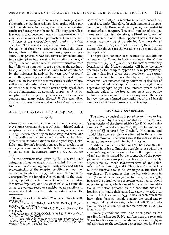
AUNIFORM color space is an arrangement ofA colors such that the intervals between the colorsappear equal. The Munsell color system' is an exampleof an approximation to a uniform color space. Undera given set of conditions (illuminant, field size, etc.),chromaticities can be assigned to the Munsell colors.When this is done, the distances between the chromatici-ties are found to be far from equal, as shown in Fig. 1.In this figure, the ovals represent loci of colors havingequal saturation (chroma) mapped onto the CIE 1931chromaticity diagram; the point near the center of theovals represents a neutral color. Clearly, the spacingbetween the ovals is not constant, even though thesaturation differences between the colors appear to beequal. Similarly, lines of equal hue (not shown) arespaced irregularly, even though the differences betweenneighboring hues appear to be roughly the same. Ap-

oij 4S00

0 05 10 IS 2 25 .30 .35 .40 .45 .585 6 5 7 7

-FIG. 1. Munsell specifications for equal color spacing plotted onthe CIE chromaticity diagram. Contours represent equal satura-tion, with chroma values as labelled. Dashed lines correspond tothe four unique hues: red, yellow, green, and blue.

' S. M. Newhall, D. Nickerson, and D. B. Judd, J. Opt. Soc.Am. 33, 385 (1943).

plication of a theorem proved by MacAdam' concerningthe variations of the magnitudes of the chromaticitysteps along certain straight lines in the chromaticitydiagram, shows that no linear transformation to anotherset of primaries can equalize the spacing between thevarious saturation and hue contours. We ask, therefore,whether a simple nonlinear transformation of the CIEchromaticity values will produce new chromaticityrepresentations which are spaced more uniformly.

Many nonlinear transformations of the chromaticitiesfor the Munsell samples have been proposed. Most ofthese transformations have been reviewed by Nickerson3and Burnham.4 Additional transformations proposedafter Burnham's evaluation include those of Godlove,5

Nickerson, Judd, and Wyszecki,6 Hurvich and Jameson,7

and Glasser et aI.8 All of these transformations have oneproperty in common: namely, a particular theoreticalframework was assumed, and the values of variousparameters were adjusted in order to give a good fitbetween theory and data. It was difficult to evaluatethe success of these various models because a measure ofgoodness-of-fit was rarely given. In contrast, the non-linear transformations described in this article werefound by keeping the theoretical constraints very loose,and by optimizing an objective measure of goodness-of-fit.

METHOD

The procedure for generating a color-vision modelfrom a given set of data is to start with a very general-ized framework which will include many specific schemesfor the mechanism of color vision. This very broadframework would have a number of free parameters, andany particular model would be described by assigningcertain values to these parameters. Because a transfor-mation of the CIE chromaticities of the Munsell sam-

2 D. L. MacAdam, J. Opt. Soc. Am. 32, 2 (1942).D. Nickerson, Paper Trade J. 125, 153 (1947).R. W. Burnham, J. Opt. Soc. Am. 39, 387 (1949).I. H. Godlove, J. Opt. Soc. Am. 42, 204 (1952).D. Nickerson, D. B. Judd, and G. Wyszecki, Die Farbe 4, 285

(1955).7 L. Hurvich and D. Jameson, J. Opt. Soc. Am. 46, 416 (1956).8 L. D. Glasser, A. K. McKinney, C. D. Reilly, and P. D.

Schnelle, J. Opt. Soc. Am. 48, 736 (1958).

1110

AUGUST I1966VOLUME 56. NUMBER 8

August1966 OPPONENT-PROCESS SOLUTIONS FOR MUNSELL SPACING

ples to a new array of more nearly uniformly spacedchromaticities can be considered isomorphic with a par-ticular model of color vision, the transformation itselfcan be used to represent the model. The very generalizedframework then becomes merely a transformation witha sufficient number of free parameters. Given the gen-eral form of the acceptable transformation, the data(i.e., the CIE chromaticities) are then used to optimizethe values of these free parameters so that the trans-formed chromaticities are as uniformly spaced as pos-sible. (This procedure was actually used by Helmholtz,9

in an attempt to find a metric for a uniform color-jndspace). The form of the generalized transformation usedhere follows an opponent-process scheme; the net inputto any one color channel is assumed to be determinedby the difference in activity between two "receptor"units. By generating such differences, the model func-tions like an instrument that measures relative values,rather than absolute values. This constraint appears tobe realistic, in view of recent neurophysiological dataon the fundamental antagonistic properties of retinalreceptive fields-a property which seems to underliecontrast and many other effects.'0-'3 The generalizedopponent-process transformation selected on this basiswas

A i= k -(aill+ aj+aj32)-kjF(bi:+ bi29+bi32) (1)

i= 1,2,3,

where A X is the activity in a color channel, the weightedx, g, 2 sums represent the spectral sensitivities of variousreceptors in terms of the CIE primaries, F is a trans-ducing function operating on these weighted sums, andki is a scaling factor corresponding to how the visualsystem weights information in the ith pathway. Helm-holtz' and Hering's formulations are both special casesof the generalized model; in Helmholtz' formulation thebij are all zero; in Hering's, only bit, bi3, a3l, a33 arezero.

In the transformation given by Eq. (1), two maincategories of free parameters can be varied: (1) the func-tion used for F (i.e., log, square root, etc.), and (2) therepresentation of the receptor sensitivities, describedby the combinations of x, g, and 2 on which F operates.Conceptually, the function F corresponds to the trans-ducing operation which converts receptor excitationinto nerve impulses, and the weighted x, y, 2 sums de-scribe the various receptor sensitivities as functions ofwavelength. Data on color matching establish that the

9 H. von Helmholtz, Sitz. Akad. Wiss. Berlin Phys. & Math.1071 (1891).

10H. B. Barlow, R. Fitzhugh, and S. W. Kuffler, J. Physiol.(London) 137, 338 (1957).

"1 D. H. Hubel and T. N. Wiesel, J. Physiol. (London) 154,572 (1960).

12H. G. Wagner, E. F. MacNichol, Jr., and M. L. Wolbarsht, J.Opt. Soc. Am. 53, 66 (1963).

13 G. Baumgartner in Neurophysiologie und Psychophysik desvisuellen Systems, edited by R. Jung and H. Kornhuber (Springer-Verlag, Berlin, 1961), pp. 296-313.

spectral sensitivity of a receptor must be a linear func-tion of x, g, and 2. Therefore, for each member of an oppo-nent pair, only three constants aij or bij are needed tocharacterize a receptor. The total number of free pa-rameters of this kind, therefore, is 18-three for each ofthe six members of the three opponent pairs. It is to beshown that the type of transducing function selectedfor F is not critical, and that, in essence, these 18 con-stants plus the ki's are the variables to be manipulatedand optimized.

The problem has now been reduced to establishinga function for F, and to finding values for the 21 freeparameters (ky, aij, bij) such that the new chromaticitylocations of the Munsell samples will have the samespacings as the samples appear to have perceptually.In particular, for a given brightness level, the satura-tion loci should be represented by concentric circleswhose radii are incremented by a fixed unit; also lines ofequal hue should correspond to radial straight linesseparated by equal angles. The unbiased procedure forassigning values to the free parameters is an iterativetechnique which minimizes the least-squares differencesbetween the transformed chromaticities of the Munsellsamples and the ideal position of each sample.

BOUNDARY CONDITIONS

The primary constraints imposed on solutions to Eq.(1) are given by the experimental data themselves.These consist of the chromaticities for 80 Munsell colorsamples [20 hues at chroma 2, 6, 10, and 14, and value(lightness)5] reported by Newhall, Nickerson, andJudd.' The color samples were limited to those withinor on the chroma-14 contour because the most extensiveobservations were conducted in this region.

Additional boundary conditions can be reasonably in-troduced in order to limit the possible values which theconstants aij, bij can assume. First, the input to thevisual system is limited by the properties of the photo-pigments, whose absorption spectra are approximatelyrepresented by linear transformations of the color-mixture functions x, g, and 2. These transformed color-mixture functions must be non-negative functions ofwavelength. This requires that the bracketed terms inEq. (1) must be non-negative for every wavelength,because the actual values represent energy absorptionsof photopigments, which cannot be negative. An addi-tional restriction imposed on the constants within abracket is to make their sum, i.e., (ajj+ai2+ai3), etc.,equal to 1.0. The equal-energy values for each bracketeditem then become equal, placing the equal-energystimulus (white) at the origin where A i= 0. This condi-tion reduces the number of free parameters ks, aij, bijfrom 21 to 15.

Boundary conditions must also be imposed on thepossible functions for F. Not all functions are relevant.These functions essentially relate increases in the physi-cal stimulus to the nonlinear representation in the re-

lilt

WHITMIAN RICHARDS

3

.6

4 6 8 10

REFLECTANCE M%)

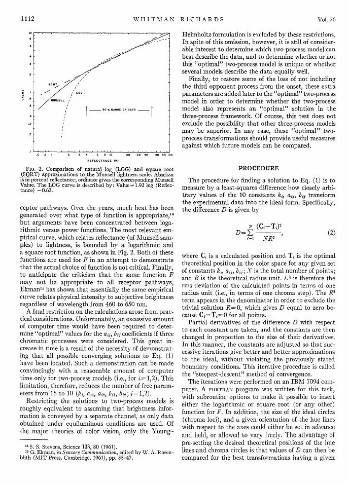
FIG. 2. Comparison of natural log (LOG) and square root(SQRT) approximations to the Munsell lightness scale. Abscissais in percent reflectance; ordinate gives the corresponding MunsellValue. The LOG curve is described by: Value= 1.92 log (Reflec-tance) -0.62.

ceptor pathways. Over the years, much heat has beengenerated over what type of function is appropriatedbut arguments have been concentrated between loga-rithmic versus power functions. The most relevant em-pirical curve, which relates reflectance (of Munsell sam-ples) to lightness, is bounded by a logarithmic anda square root function, as shown in Fig. 2. Both of thesefunctions are used for F in an attempt to demonstratethat the actual choice of function is not critical. Finally,to anticipate the criticism that the same function Fmay not be appropriate to all receptor pathways,Ekman" has shown that essentially the same empiricalcurve relates physical intensity to subjective brightnessregardless of wavelength from 460 to 650 nm.

A final restriction on the calculations arose from prac-tical considerations. Unfortunately, an excessive amountof computer time would have been required to deter-mine "optimal" values for the aij, bij coefficients if threechromatic processes were considered. This great in-crease in time is a result of the necessity of demonstrat-ing that all possible converging solutions to Eq. (1)have been located. Such a demonstration can be madeconvincingly with a reasonable amount of computertime only for two-process models (i.e., for i= 1,2). Thislimitation, therefore, reduces the number of free param-eters from 15 to 10 (ki, a,,, ai2 bil, bi2; i= 1,2).

Restricting the solutions to two-process models isroughly equivalent to assuming that brightness infor-mation is conveyed by a separate channel, as only dataobtained under equiluminous conditions are used. Ofthe major theories of color vision, only the Young-

4 S. S. Stevens, Science 133, 80 (1961).G6 C. Ekman, in Sensory Communication, edited by W. A. Rosen-

blith (MIT Press, Cambridge, 1961), pp. 35-47.

Helmholtz formulation is excluded by these restrictions.In spite of this omission, however, it is still of consider-able interest to determine which two-process model canbest describe the data, and to determine whether or notthis "optimal" two-process model is unique or whetherseveral models describe the data equally well.

Finally, to restore some of the loss of not includingthe third opponent process from the onset, these extraparameters are added later to the "optimal" two-processmodel in order to determine whether the two-processmodel also represents an "optimal" solution in thethree-process framework. Of course, this test does notexclude the possibility that other three-process modelsmay be superior. In any case, these "optimal" two-process transformations should provide useful measuresagainst which future models can be compared.

PROCEDURE

The procedure for finding a solution to Eq. (1) is tomeasure by a least-squares difference how closely arbi-trary values of the 10 constants ki, aij, bij transformthe experimental data into the ideal form. Specifically,the difference D is given by

Nf (Ci-T )2(2

N R2

where Ci is a calculated position and Ti is the optimaltheoretical position in the color space for any given setof constants k,, aij, bij; V is the total number of points;and R is the theoretical radius unit. L ' is therefore therms deviation of the calculated points in terms of oneradius unit (i.e., in terms of one chroma step). The RIterm appears in the denominator in order to exclude thetrivial solution R=0, which gives D equal to zero be-cause Ci=Ti=0 for all points.

Partial derivatives of the difference D with respectto each constant are taken, and the constants are thenchanged in proportion to the size of their derivatives.In this manner, the constants are adjusted so that suc-cessive iterations give better and better approximationsto the ideal, without violating the previously statedboundary conditions. This iterative procedure is calledthe "steepest-descent" method of convergence.

The iterations were performed on an IBM 7094 com-puter. A FORTRAN program was written for this task,with subroutine options to make it possible to inserteither the logarithmic or square root (or any other)function for F. In addition, the size of the ideal circles(chroma loci), and a given orientation of the hue lineswith respect to the axes could either be set in advanceand held, or allowed to vary freely. The advantage ofpre-setting the desired theoretical positions of the huelines and chroma circles is that values of D can then becompared for the best transformations having a given

1112 Vol. 56

August1966 OPPONENT-PROCESS SOLUTIONS FOR MUNSELL SPACING

relationship to one another. Such comparisons providean estimate of the accuracy and uniqueness of any"best" transformation. The importance of these varia-tions in D for different transformations becomes clearerwhen specific examples are presented.

In order to converge onto the best possible solutionfor Eq. (1), the problem was broken up into severalstages. First, D values were calculated for the besttransformations to various ideal solutions having fixedradii and fixed hue lines, and with scale coefficients ksconstant, but not necessarily the same. These fixed idealsolutions were systematically related so that a profileof D could be obtained showing the extent of conver-gence when a given hue and chroma value (5PB/10)was held at a certain position with respect to the axesA1, A2. Contours of equal D could then be drawn, in-dicating how rapidly D varied as the 5PB/10 positionin the color space was changed. As a result, the topo-graphy indicated regions of minimum D where conver-gence to a "best" solution would be expected.

Even though the construction of such a profile mapwas necessary in order to determine the number of pos-sible solutions to Eq. (1), the computation time requiredto do this in all cases was prohibitive, in spite of the factthat only 16 points (based on hues: 5PB, 10G, 5Y,1ORP) were used. As an alternative, therefore, laterprofile runs kept the radius of the ideal circles constant,and changed only the angular position of the hue lineswith respect to the axes. By allowing the scale coeffi-cients ki to vary also, the fixed-radius constraint did notcause distortions in the calculated values of the param-eters ai1, bhj. D values could then be plotted as a uni-dimensional function of the angular position of the pointSPB/10. Twenty points (based on hues: 5PB, 5BG,5GY, 5YR, 5RP) were used for these unidimensionalprofile runs.

Once the regions of minimum D were determined,the number of points to be transformed was increased,and convergence was continued to find the minimizingsolutions. For these final converging operations, no con-straints were imposed on the position of the pointSPB/10. The results gave the best two-dimensionaltransformation for the Munsell data.

The second phase of the problem involved a limitedsearch for a three-dimensional planar solution. In otherwords, the values of A 1, A 2, A 3 were calculated for each.Munsell color; then the best regression plane throughall the points defined by A1, A2, A3 was determined.Each individual point was then projected onto thisplane. The ordinate on the regression plane was arbi-trarily taken as the line which joined the projectedneutral point with the point of intersection of A1 andthe regression plane. The abscissa was made perpendi-cular to this ordinate. For these calculations, the besttwo-dimensional transformation was used as a first ap-proximation, in order to determine whether increasingthe number of free parameters from 10 to 15 would alterthe solutions.

LOG FUNCTION

....

'.4

-- \ .- N

-e ''/ / /

SORT FUNCTION

...

!

; I.,.. o ,o

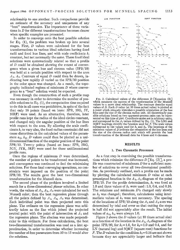
FIG. 3. Calculated values of the difference D [Equation (2)]which measures the success of the tranformation of the Munsellvalues to a more ideal relationship. The contours describe equalvalues of D. Each D value (at 10 times actual value) is plotted ata point which uniquely identifies a possible orientation of the huelines and the size of the chroma radius unit. All theoretically pos-sible solutions based on two opponent-process pairs can be repre-sented on this type of plot. Coordinate scales are in arbitrary units,and correspond to the Ai values defined by Eq. (1). The LOG andSQRT headings identify the function used for F. The scale valuescorrespond to the values used for ki and k2. The locations of theminimum values of D indicate the orientation of the hue lines andthe size of the chroma radius unit which will provide the besttransformation of the Munsell data for 4 hues and 4 chromas.

RESULTS

1. Two Chromatic Processes

As a first step in examining the possible transforma-tions which minimize the difference D [Eq. (2)], a pro-file was constructed of minimum D for a sufficient num--ber of solutions to cover all two-dimensional possibili-ties. As previously outlined, such a profile can be madeby plotting the calculated minimum D value at eachpreassigned location in the A 1, A 2 diagram of the point5PB/10. For the profile determination, k1 was fixed at1.0 and three values of k2 were used: 1.0, 0.4, and 0.16.The solutions and minimum D's changed only slowlyas k2 was changed; therefore, calculations using inter-mediate values of k2 were not necessary. The spacingof the locations of 5PB/10 along the A 1 and A 2 axes wasdetermined by trial and error so that cutting the stepsin half did not appreciably alter the result. The initialvalues of anj, bij were always 1.0.

Figure 3 shows the D values (at 10 times actual size)as a function of the location in the A 1, A 2 diagram of thepoint SPB/10, for kl= 1.0, for k2= 1.0 and 0.4, and forLN (natural log) and SQRT (square root) functions forF. The D values for the condition k2 = 0.16 are not shownbecause they are appreciably larger and indicate that

1113

WHITMAN RICHARDS

TABLE I. Solutions and optimum parameters for uniform Munsell spacing.

Solution Angle Difference Scale Calculated constantstype Function (deg) (D) coeff. ail ai2 aj3 bil bi2 bi3

2D-10 LN 67.5 0.31 1.0 0.73 0.21 0.06 -0.24 1.08 0.24(4 hues) 1.0 -0.23 1.18 0.07 0.26 0.41 0.48

22.5 0.33 1.01.0

56 0.47 1.01.0

0 0.60 1.01.0

45 1.8 1.0

67.5

0.4

1.8 1.00.4

92 1.5 0.791.06

83 1.5 0.800.94

74 0.81 0.900.97

65 0.87 0.940.90

55 1.6 1.410.81

47 1.8 0.901.02

38 1.7 0.910.66

30 1.75 0.920.55

20 2.7 0.980.47

12 2.9 0.980.68

0.71-0.47

0.850.77 -

0.01-0.42

0.70

-0.460.360.98 -

-0.13-0.43-0.19-0.43-0.25-0.40-0.30-0.36-0.30-0.31-0.34

0.30

-0.450.26

-0.440.59

-0.321.03

-0.450.80

0.30 -0.05 0.35 0.361.40 0.10 0.73 0.08

0.04 0.12 0.34 0.33-0.08 0.42 -0.18 1.01

0.87 0.16 0.07 0.461.33 0.14 0.92 -0.01

0.22 0.08 0.28 0.47

1.37 0.09 0.44 0.13

0.32 0.44 0.08 0.73-0.06 0.09 -0.04 0.80

0.841.38

0.961.37

1.081.35

1.161.31

1.141.27

1.210.68

1.400.76

1.390.44

1.270.03

1.400.20

0.420.08

0.340.08

0.260.08

0.710.24

0.730.16

0.740.13

0.280.51

0.250.53

0.240.54

0.20 0.73 0.240.07 0.05 0.57

0.25 0.50 0.390.06 -0.11 0.66

0.190.02

0.09-0.03

0.09-0.07

0.07-0.13

0.090

0.850.37

0.680.10

0.670.11

0.770.10

0.650.10

0.040.32

0.240.46

0.200.42

0.080.42

0.250.50

72 1.2 3.1 -0.32 1.15 0.24 1.00 -0.01 -0.033.9 -0.34 1.24 0.15 0.19 0.43 0.55

64 1.1 3.63.7

57 0.85 3.32.7

46 1.2 3.83.7

34 1.35 3.93.5

29 2.0 4.74.0

11 1.75 4.44.0

3 1.6 4.24.2

-6 1.3 3.94.7

-14 1.25 3.65.3

-25 1.3 2.85.2

-0.34-0.24-0.24-0.25-0.35

0.02

-0.350.16

-0.210.76

-0.200.88

-0.220.94

-0.260.95

-0.220.96

-0.250.98

1.201.14

1.211.20

1.240.87

1.250.73

1.060.11

1.060.03

1.09-0.03

1.13-0.05

1.09-0.07

1.13-0.08

0.200.16

0.050.08

0.170.15

0.160.15

0.230.16

0.210.11

0.200.09

0.190.12

0.190.11

0.180.11

0.980.13

1.090.23

0.900.06

0.840.03

0.800.33

0.700.32

0.630.25

0.540.17

0.480.19

0.300.19

-0.010.44

-0.080.26

0.000.47

0.020.50

-0.020.25

0.010.33

0.040.44

0.080.56

0.090.59

0.150.62

0.010.63

-0.050.75

0.110.69

0.180.69

0.300.60

0.400.51

0.460.45

0.540.38

0.610.31

0.780.25

SQRT

LN

SQRT

2D-10(5 hues)

LN

0.400.25

0.4g0.24

C.680.11

0.25

0.42

0.270.34

-0.020.36

00.441

0.010.47

0.030.54

0.140.67

0.130.45

0.090.63

0.170.69

0.190.70

0.100.60

SQRT

1114 Vol. 5 6

Augustl966 OPPONENT-PROCESS SOLUTIONS FOR MUNSELL SPACING

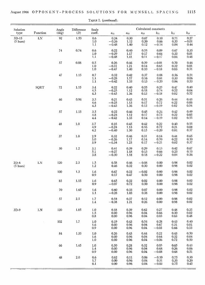
TABLE I. (continued).

Solution Angle Difference Scale Calculated constantstype Function (deg) (D) coeff. ail ai2 ab3 bi 3 bi2 bj3

3D-15 LN 92 1.55 0.6 0.24 0.30 0.67 0.10 0.71 0.27(5 hues) 1.0

1.1

74 0.74 0.61.01.1

57 0.88 0.51.01.0

47 1.15 0.71.11.1

72 1.15 3.44.54.3

66 0.96 3.54.64.3

57 1.15 3.54.84.4

48 1.0 3.74.94.2

37 1.0 2.95.03.9

30 1.2 3.15.13.8

120 2.3 1.51.2

0.20 0.66 0.33 -0.010.12 -0.14 0.84 0.44

0.09 0.670.64 0.33

-0.17 0.84

-0.010.65

-0.18

0.700.320.83

0.550.170.11

0.390.140.10

-0.26 1.12-0.48 1.40

0.22 0.40-0.29 1.17-0.48 1.41

0.26 0.46-0.31 1.21-0.47 1.40

0.32 0.42-0.28 1.17-0.42 1.33

0.22 0.40-0.25 1.12-0.45 1.36

0.21 0.43-0.25 1.13-0.45 1.36

0.22 0.46-0.24 1.12-0.42 1.33

0.37 0.08 0.560.16 0.61 0.330.13 -0.20 0.84

0.550.180.13

0.510.170.13

0.450.170.14

0.25 0.45 0.42-0.24 1.13 0.16-0.40 1.30 0.15

0.32 0.46 0.31-0.26 1.17 0.14-0.34 1.23 0.17

0.41 0.39-0.27 1.18-0.30 1.18

0.290.130.18

0.25 0.470.74 0.22

-0.18 0.82

0.260.72

-0.19

0.440.220.82

0.24 0.420.73 0.22

-0.19 0.82

0.220.72

-0.20

0.140.70

-0.21

0.400.210.81

0.410.220.82

0.13 0.420.66 0.23

-0.22 0.84

0.58 0.46 -0.08 0.00 0.98 0.020.46 0.32 0.30 0.00 0.98 0.02

100 1.3 1.6 0.67 0.32 -0.02 0.00 0.98 0.020.9 0.17 0.47 0.50 0.00 0.98 0.02

85 1.15 1.6 0.65 0.32 0.02 0.00 0.98 0.020.9 -0.07 0.72 0.50 0.00 0.98 0.02

70 1.65 1.6 0.60 0.33 0.07 0.00 0.98 0.021.1 -0.28 1.03 0.38 0.00 0.98 0.02

57 2.5 1.7 0.54 0.37 0.12 0.00 0.98 0.021.4 -0.38 1.21 0.26 0.00 0.98 0.02

120 1.85 1.01.50.8

102 1.7 1.01.60.9

84 1.35 1.01.61.0

66 1.45 1.01.40.9

48 2.0 0.61.70.1

0.18 0.39 0.620.00 0.96 0.040.00 0.96 0.04

0.19 0.43 0.540.00 0.96 0.040.00 0.96 0.04

0.26 0.43 0.440.00 0.96 0.040.00 0.96 0.04

0.50 0.28 0.320.00 0.96 0.040.00 0.96 0.04

0.82 0.110.00 0.960.00 0.96

0.27 0.480.66 0.300.03 0.63

0.280.67

-0.03

0.220.64

-0.06

0.050.68

-0.08

0.430.310.66

0.430.320.72

0.650.260.68

0.06 -0.10 0.750.04 0.51 0.350.04 -0.03 0.75

0.350.010.48

0.440.010.51

0.510.060.53

0.400.040.52

0.430.060.54

0.490.050.55

0.550.080.57

0.650.100.57

0.670.130.56

SQRT

2D-6(5 hues)

LN

3D-9 LN 0.350.020.48

0.400.010.53

0.500.040.50

0.430.060.51

0.500.200.45

1115

WHITMAN RICHARDS

4030

20

to

4-

20

10

-OG FUN.ICTONi S99T FUNCTION

90 72 54 36 IS 0 72 54 06 IN 0 -l'

ZD-I1

//

x - 15 -

\ ,/ t5HUES)

90 72 54 36 18 0 72 54 36 18 0 -lB

LOG FUNCTION

60 .2D - 6 3D-9

40 - 15 HUES) (5 HUES)

30-20- / _

10935 117 99 SI 63 45 117 99 NI 69 45 27

ANGLE (DEC.)

FIG. 4. Minimum values of D (at X 10) for fixed angular posi-tions of the point SPB/10. Each point corresponds to a possibleorientation of the hues with respect to the A, axis. The D valuesshow the success of the best transformation of the Munsell datawhich approximate the given orientation of the hue lines, indi-cated by the angular position of 5PB shown on the abscissa. The2D-10 curves describe the results for two opponent-process pairswith a total of 10 free parameters corresponding to ad1, bij in Eq.(1). The 4-hue curves are taken from Fig. 3. The 3D-15 curvesdescribe the results for three opponent-process pairs with 15 freeparameters. The headings in the lower portion of the figure re-spectively correspond to two and three opponent-process pairswith 6 and 9 parameters. See text and Table I.

no optimal solution is present in this region of the solu-tion space.

The upper half of Fig. 3 shows the minimum D valueswhen ki= 1.0 and k 2 = 0.4. At this level in the solutionspace, the best approximation gives a D of 1.8 for boththe LN function (at 450 from the horizontal A 1 axis) andfor the SQRT function (at 56°). The correspondingoptimum values of the constants aii, bij are given inTable I, listed under solution-type 2D-10 (4 hues).These values should be compared with the best solu-tions obtained when the scale coefficients k1, k2 are both1.0. The lower half of Fig. 3 shows that under theseconditions D can be minimized in two regions. For theLN function, D is about 0.31 at 67.50 from the hori-zontal axis and 0.33 at 22.50. Somewhat larger valuesof 0.47 and 0.60, at 560 and 30, are found when theSQRT function is used. These solutions are also givenin Table I, listed under solution-type 2D-10 (4 hues).

Three important observations can be made aboutthese profile calculations. First, the LN and SQRT func-tions do not give appreciably different optimal solutions.Even though the angular positions of the minima andthe contours are disLorLed, the general relalionships be-tween points remain preserved. Secondly, there appearto be two regions where D can be minimized, givingtentative solutions of:

I

Solution 1:

A 1= F(0.80.+0.10y+0.002)

-F(- 0.30t+ 1.200+0.202)

A 2= F(- 0.10+ 1.000+0.102)- F(0.1Ox+0.45g+0.552)

Solution 2:

l I'= F(0.752+0.00g+0.352)- F(- 0.37f+ 1.209 +0.152)

A 2'= F(0.S80 +0.209+0.05 )-F(0.3 5;+0.359+0.452). (3b)

The constants in the above solutions are rough averagesof the LN- and SQRT-function values. (The order ofthe pairs of functions has been changed from that givenin Table I to facilitate comparison.) The third observa-tion is that when k2 is changed from 1.0 to 0.4, there isonly a small effect on the constants of the resultantsolution. (Refer to Table I.) Therefore, in spite of thelarge distortion in the scale of the axes A l, A 2, the cal-culated solutions change only slowly, thereby causingthe increase in the D values. This shows that the regionsof true minima in the solution space lie near to theplane where ki= k2 = 1.0.

A further factor affecting the resultant solutions is thenumber of data points used as boundary conditions. Inthe case where 4 hues only are used, as was dictated bythe available computation time, the boundary condi-tions are rather loose. For instance, the restriction thatthe chroma contours be circular cannot be enforced,for either a circle or a square shape might equally wellfit the 4 hue points at equal chroma. In fact, if pointsbetween the 4 hue positions are plotted, they do tendto be displaced away from the ideal circular form towardthe origin, showing that the 4-hue solution is actuallysomewhat rectilinear. If the number of hues is increased,therefore, the solutions might be expected to change.In spite of such changes, however, very likely thereshould be no increase in the number (or relative posi-tion) of the regions of minimal D. If anything, additionalconstraints should tend to eliminate some of theseregions.

In order to investigate the effect of increasing thenumber of data points, and to converge onto a bettersolution, the number of hues was increased from 4 (16points) to 5 (20 points). Rather than running a com-plete profile, as was done in constructing Fig. 3, con-vergence was made to that solution which minimizedD, for each of a number of assigned angular positionsof SPB/10. The radius was held fixed for these calcula-tions; consequently, it was necessary to vary the scalecoefficients le, and k2. Therefore, the unit along eachaxis A1 and A12 could be different. The resultant Dvalues for different angular positions of the point5PB/10 are given in Fig. 4 in the top two curves, cate-gorized as 2D-12. The 4-hue curve is merely a replot of

1116 Vol. 56

(3a)

August1966 OPPONENT-PROCESS SOLUTIONS

the lowest D values taken from Fig. 3, with k2= 1.0.When 5 hues are used, these lowest D values are in-creased to the new values given in the top curve labelled"5 hues." The increase in the number of data pointseliminated the "rectilinear" form of the solutions andraised D. In spite of this increase, however, the regionsof minima remain at approximately the same angularlocations of the hue lines. The solutions for this 5-huecondition are listed in Table I. These solutions retainthe same form and are similar to those given for the4-hue condition.

Finally, to determine the best two-dimensional trans-formation of the Munsell data, the number of hues wasincreased to 10 and then to 20, giving a total of 77points. As the number of data points was increased, theD values for the solution (2) became increasingly higherrelative to those of solution (1). This trend was alreadyapparent in Fig. 4, particularly for the log function. Thebest solution, to which all others in the neighborhoodconverged, was found to be:

A 1=1.0 In (0.586?+0.390g+0.012z)

-1.0 ln(- 0.050s+0.9731+0. 1072)

A 2=1.0 ln(-0.175&+0.931y+0.3572)-1.0 ln(-0.3 8 5±+1.33 8V+0.0 7 32) (4)

with D = 0.38. (Note that ki = k2= 1.0). When the SQRTfunction was used, a very similar solution was also ob-tained, but with a higher D, 0.75.

For 20 hues, solution (2) resulted in the followingconstants:

A1 =3.9 SQRT(-0.25x+1.132+0.182)-3.9 SQRT(0.48&+0.08i+0.622)

A2=5.4 SQRT(0.90;+0.00y+0.112)-5.4 SQRT(0.18&+0.59p+0.332) (5)

with D= 1.3 for SQRT and 2.0 for LN functions. Be-cause solution (2) gave a much poorer approximation tothe ideal color space, as indicated by the large D, itwas discarded.

The best two-dimensional transformation is plottedin Fig. 5. Each axis represents one of the pairs of func-tions in Equation (4), and the axis scales are in chromaunits. The large circles and the radial lines are thetheoretical positions for the equally spaced colors. Thesmall circles indicate the transformed chromaticityvalues. The outer, curved boundary is the spectral locus.Significant discrepancies in the calculated values appearonly near 5G, chroma 10 to 14, and 5Y, chroma 6.

Solution (1) has been dubbed "Muller-Judd," aslabeled in Fig. 5, because if the LN function in Eq. (4)is omitted and linear comparisons are made, then the(equal energy) axis values become

A 1 (linear) = 0.64x- 0.58p- 0.092,

A 2 (linear) = -0.212+0.41p-0.282. (6)

AZ

A,

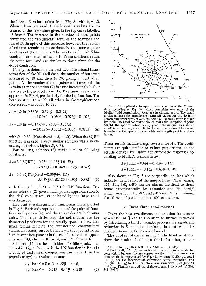
FIG. 5. The optimal color-space transformation of the Munselldata according to Eq. (4), which resembles one stage of theMiiller-Judd formulation. Axes are in chroma units. The smallcircles indicate the transformed Munsell values for the 20 huesshown and for chroma of 2, 6, 10, and 14. The ideal array is givenby radial lines and concentric circles. With the exception of pointSG/14, the approximation is very good. The unique hues, shownat 900 to each other, are at 60° to the coordinate axes. The curvedboundary is the spectral locus, with wavelength positions givenin urn.

These results include a sign reversal for -42. The coeffi-cients are quite similar to values proportional to theresults derived by Judd"6 for chromatic responses ac-cording to Muller's formulation":

A j(Judd) = 0.64x-0.51-0.132,A 2 (Judd) = -0. 15.t+0.43y-0.282. (7)

Also shown in Fig. 5 are perpendicular lines whichindicate the location of the unique hues. These values,477, 514, 580, c.495 nm are almost identical to thosefound experimentally by Dimmick and Hubbard,1 8

which were 475, 515, 582, and c.495 nm. Note, however,that these unique colors lie at 60° to the axes.

2. Three Chromatic-Processes

Given the best two-dimensional solution for a colorspace EEq. (4)], can this solution be further improvedby introducing a third chromatic process? If a significantreduction in D could be obtained, then this would beevidence favoring three color-channels.

The third set of curves in Fig. 4, identified as 3D-15,show the results of adding a third dimension, or axis

"D. B. Judd, J. Res. Natl. Bur. Stds. 42, 1 (1949)."Technically, Eq. (6) supports only the Schrddinger model for

color vision, because this model proposes that the final color sensa-tions would be represented by Eq. (4), whereas Mtller proposedEq. (4) for the intermediate chromatic retinal responses, andEq. (8) (Hering) for the final chromatic sensations. (See Judd.2 0 )

18 F . L. Dimmick and M. R. Hubbard, Am. J. Psychol. 52, 242,348 (1939).

FOR MUNSELL SPACING 1117

11181WHITMAN RICHARDS

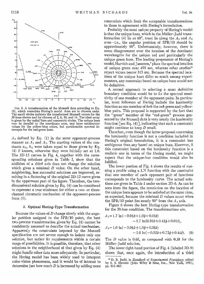
FIG. 6. A transformation of the Munsell data according to Eq.(8), which resembles Hering's model. Axes are in chroma units.The small circles indicate the transformed Munsell values for the20 hues shown and for chroma of 2, 6, 10, and 14. The ideal arrayis given by the radial lines and concentric circles. The unique huesnow lie parallel to the coordinate axes, and have satisfactoryvalues for the yellow-blue colors, but questionable spectral in-tercepts for the red-green hues.

A s defined by Eq. (1) in the same opponent-processmanner as AX and A42. The starting values of the con-stants ai1, bij were taken equal to those given by Eq.(4) if known, otherwise they were initially set at 1.0.The 3D-15 curves in Fig. 4, together with the corre-sponding solutions given in Table I, show that theaddition of a third axis does not change the solutionwhich gives a minimal D value. On the other hand,neighboring, less successful solutions are improved, re-sulting in a flattening of the original 2D-12 curve givenin the uppermost part of the figure. Therefore, the two-dimensional solution given by Eq. (4) can be consideredto represent a true minimum for either a two- or three-channel chromatic mechanism of the opponent-processform (1).

3. Optimal Hering-Type Transformation

Because the values of D change slowly with the angu-lar position assigned to the 5PB/10 point, the besttwo-process transformation given by Eq. (4) cannot beconfidently assumed to describe the actual mechanism.Apparently the constraints imposed by the Munsellspecification are not severe enough to isolate only onesolution, but rather fix requirements within a certainrange of possibilities. It is possible, therefore, that othersolutions in the neighborhood of that given by Eq. (4)might handle other data more adequately. In particular,the Hering model has been widely used to interpretcolor-vision phenomena, and it would be of interest todetermine just how much D is increased by adding more

constraints which limit the acceptable transformationsto those in agreement with Hering's formulation.

Probably the most unique property of Hering's modelis that the unique hues, which in the MUller-Judd trans-formation (4) lie at 600, must lie along the AI and A2axes-i.e., the angular position of 5PB/10 should beapproximately 900. Unfortunately, however, there issome disagreement over the location of the dominantwavelengths for the unique red and particularly theunique green hues. The leading proponents of Hering'smodel, Hurvich and Jameson,7 place the spectral locationof unique green near 495 nmm whereas other studies'report values nearer 515 nm. Because the spectral loca-tions of the unique hues differ so much among experi-menters, any constraint based on unique hues would notbe definitive.

A second approach to selecting a more definitiveboundary condition would be to fix the spectral sensi-tivity of one member of the opponent-pairs. In particu-lar, most followers of Hering include the luminosityfunction as one member of both the red-green and yellow-blue pairs. This proposal is supported by the fact thatthe "green" member of the "red-green" process gen-erated bv the Munsell data is very nearly the luminosityfunction [see Eq. (4)], indicating that such a constraintmight continue to keep D small.

Therefore, even though the latter proposal concerningthe luminosity function is not a condition included inHering's original for-mulation, it is a constraint lessambiguous than any based on unique hues. However, ifthis constraint based on the luminosity function is arealistic one in terms of the Hering model, we mightexpect that the unique-hue condition would also befulfilled.

The lower portion of Fig. 4 shows the results of run-ning a profile using a LN function with the constraintthat one member of each opponent pair of functionscorresponds to the luminosity curve. The actual solu-tions are given in Table I under section 2D-6. As can beseen from the figure, the restriction on the location ofthe unique hues appears to be satisfied at the same time,as expected, because the minimal D values occur whenthe 5PB/10 point lies nearly 90° from the A 1 axis.

Figure 6 shows the best Hering-type transformationfor the 20-hue condition. The transformations are,

AI= 1.7 ln(-0.0lxt+1.O&+0.012)-1.7 In(0.56? +0.41l+0.0Ul),

A1 2= 1.0 ln(-0.0I 2+1.Oij-VO.012)-1.0 In(-0.02x+0.72p+0.442). (8)

The D value is 0.65, as compared with 0.38 for theMuller-Judd solution.

The lower right-hand portion of Fig. 4 (labeled 3D-9)shows that, once again, the introduction of a third

19 D. B. Judd, in Habdbook of Experimental Psychology, editedby S. S. Stevens (John Wiley & Sons, Inc., New York, 1951),pp. 811-867.

1118 Vol. 56

August1966 OPPONENT-PROCESS SOLUTIONS FOR -MUNSELL SPACING

chromatic-process A3 has no effect on the position ofthe minimum, but merely reduces the neighboring Dvalues as compared with the two-dimensional case.Therefore, with the additional constraint that one mem-ber of each chromatic pair be the luminosity function,the Hering model, which postulates only two chromatic-processes, still seems to give a true minimum for D evenif an extra chromatic process (plus a separate lightnessmechanism) is assumed.

DISCUSSION

Several assumptions were necessary in order to deter-mine an "optimal" transformation of the chromaticityvalues of the Munsell samples to a more uniform co-ordinate system. Of these, the one most subject toquestion is probably the assumption that the Munsellsystem represents uniform spacing of colors. Recentevidence suggests that the Munsell samples may be onlya first approximation?0 Because calculations were notperformed to determine the effects of data distortion,it is not known how sensitive the final solutions are toirregularities in the spacing.

In spite of this uncertainty, however, the form of theoptimal two-process transformation given by Eq. (4)is quite surprising. We must remember that there wasno constraint to guarantee that a "reasonable" solutionwould be obtained. Nevertheless, at least two propertiesof the solution (4) appear "reasonable." First, most ofthe spectral sensitivities of the members of each pairagree well with similar functions determined in otherways. Secondly, the final solution (4) agrees with onepossible model for color vision proposed on completelydifferent grounds. Particularly surprising is the resultthat to a first approximation each channel is given equalweight (i.e., kl-k 2). The transformation given by Eq.(4), therefore, can be considered as evidence favoringa Muller, or, more correctly, a Schrddinger model ofcolor vision.1 7

On the other hand, if evidence from other sourcesrequires that any model for color vision be in agreementwith a Hering model, then Eq. (8) might be consideredas a good quantitative model, qualified again by howmuch confidence can be placed in the Munsell spacing.

Both Eqs. (4) and (8) have a property in commonwhich may be significant. In both transformations, the"blue" member of the "yellow-blue" pair is composedof the tristimulus function "2" (considered approxi-mately characteristic of the short-wave pigment 440),plus the luminosity function "f". This suggests thatthe input to the visual system from the 440 receptor maybe desaturated by the two other cone systems, 540 and580. That the outputs from several cones of differenttypes may converge onto one channel is a likely pos-sibility, considering the 6 to 1 ratio between cones andoptic-nerve fibers. Therefore, we should not immedi-

20 D. B. Judd, J. Opt. Soc. Am. 45, 673 (1955).

ately exclude a multi-peak sensitivity function as ab-normal, unless the peaks disagree with those determinedfrom photopigment absorption curves or from relevantpsychophysical experiments.

A final point of interest is the unusual angular posi-tion of the unique hue lines when the t ivIiller-Judd"transformation (4) is used. This is particularly surpris-ing, when we consider how closely these perpendicularlines approximate the average spectral locations of theunique hues found by Dimmick and Hubbard."8 Thisanomaly could, of course, be due to some kind of sys-tematic irregularity in the Munsell spacing. On theother hand, it is also possible that the apparent rotationof the unique hues is a result of confining the transfor-mation to two opponent-processes. In this case, theresultant solution (4) might represent a planar projec-tion of a more suitable three-process model. Preliminarycalculations using three chromatic-pairs show that thetheoretical anomalies of the Muller-Judd solution (4)can be overcome. The three-pair model assumes thatthere are three chromatic channels (plus one achromaticchannel) constructed from all opposing pairs of the R,G, and B response functions: R:G, G:B, and B:R. Ap-propriate functions for R, G, and B are:

R= 0.70Z+0.339-0.082G= -0.42Z+ 1.36gy0.092B= -0.12x+0.88v+0.352. (9)

The triple-pair solution based on these primaries anda log-transformation function is almost identical to Fig.5, except that the Al and A2 axes now lie in the direc-tion of the unique hues. The rms D value is about 0.6.

CONCLUSIONS

Equations {4), (8), and (9) show that "reasonable"solutions for a color space can be derived in an unbiasedway using a simple opponent-process model and datadescribing uniform color spacing. With a limited numberof constraints and 10 free parameters, the Munsellspacing was best described by a transformation fittinga Muller-Judd, or particularly the Schrddinger scheme.However, when the number of free parameters wasreduced to 6 by the additional requirement that theluminosity function be included as one member of eachopponent-pair, a Hering transformation was found tobe optimal. These two different solutions demonstratethat by appropriately selecting the constraints, theresultant optimal transformation can be manipulatedsomewhat. Therefore, the confidence we can place inthe derived solutions seems to depend not so much uponthe method itself, but rather upon the assumptions andthe data which provide the constraints. By adding onlyone or two items to our collection of "irrefutable"quantitative constraints, we may be able to apply thesame method to reach a more definitive conclusion.

1119

WHITMAN RICHARDS

ACKNOWLEDGMENTS

Professor H.-L. Teuber, Professor R. Held, and Pro-fessor W. Wickelgren, and Dr. D. L. MacAdam ofEastman Kodak Co. all provided helpful criticisms ofthe text, and their comments clarified considerably thepresentation of the material.

During this project, the author received a pre-doctoralfellowship from the National Institute of General Medi-

cal Sciences under grant 5TlGM-1064-03 and additionalsupport under grant NsG 496 from the National Aero-nautics and Space Administration to Professor H.-L.Teuber, MIT Psychology Department, Cambridge,Mass.

The calculations were performed on an IBM 7094computer at the MIT Computation Center, Cambridge,Massachusetts.

1120 Vol. 56