Embed Size (px)
Citation preview
www.cpc-analytics.com | [email protected]
Operationalizing algorithmic explainability in the context of risk profiling done by robo financial advisory apps.
Research Paper | 8th December 2019
Sanjana Krishnan, Sahil Deo, Neha Sontakke
Abstract
Risk profiling of users is of functional importance and is legally mandatory for each robo
financial advisor. Irregularities at this primary step will lead to incorrect recommendations for
the users. Further, lack of transparency and explanations for automated decisions makes it
tougher for users and regulators to understand the rationale behind the decisions made by the
apps, leading to a trust deficit. Regulators closely monitor this profiling but possess no
independent toolkit to “demystify” the black box or adequately explain the decision-making
process of the robo financial advisor.
Our paper argues the need for such a toolkit and proposes an approach towards developing it.
We use machine learning models to deduce an accurate approximation of the robo advisory
algorithm and provide three levels of explanation. First, we reverse engineer the model to find
the importance of inputs. Second, we infer relationships between inputs and with the output.
Third, we allow regulators to explain decisions for any given user profile, in order to ‘spot
check’ a random data point. With these three explanation methods, we provide regulators, who
lack the technical knowledge to understand algorithmic decisions, a toolkit to understand it and
ensure that the risk-profiling done by robo advisory apps comply with the regulations they are
subjected to.
Keywords: Algorithmic decision-making systems (ADS), algorithmic regulation, algorithmic
explainability and transparency, robo financial advisory apps, fintech, explainable AI, Machine
Learning
Introduction
There is a growing ubiquity of decision-making algorithms that affect our lives and the choices
we make. These algorithms curate our internet and social media feed, trade in the stock market,
assess risk in banking, fintech and insurance, diagnose health ailments, predict crime
prevention, and a lot more. Broadly, these are known as Algorithmic Decision-making Systems
(ADS). Machine learning algorithms are the backbone of ADS and artificial intelligence (AI),
www.cpc-analytics.com | [email protected]
and power the automated, independent decision making done by computers. Machines ‘learn’
by going through millions of data points and find associations and patterns in them. They then
apply the learnt rules on new data to predict the outcomes. These algorithms have promised
and delivered considerable gains in efficiency, economic growth, and have transformed the
way we consume goods, services, and information.
However, along with the gains, these algorithms also pose threats. Several cases have come to
light where algorithm powered decisions have given rise to undesirable consequences. An
automated hiring tool used by Amazon discriminated heavily against women applying for
software development jobs, because the machines learn from past data which has a
disproportionate number of men in software positions (Dastin, 2018). Software used for crime
prediction in the United States showed a machine bias against African-Americans,
exacerbating the systemic bias in the racial composition of prisons (ProPublica, 2016).
Google’s online advertising system displayed ads for high-income jobs to men much more
often than it did to women (Datta, Tschantz, & Datta, 2015). Social media algorithms are found
to inadvertently promote extremist ideology (Costello, Hawdon, Ratliff, & Grantham, 2016)
and affecting election results (Baer, 2019). Recently, researchers found that racial bias in the
US health algorithms reduced the number of Black patients identified for extra care by more
than half (Obermeyer, Powers, Vogeli, & Mullainathan, 2019) (Kari, 2019).
In effect, contrary to the promise of unbiased and objective decision making, these examples
point to a tendency of algorithms to unintentionally learn and reinforce undesired and non-
obvious biases, thus creating a trust deficit. This arises mainly because several of these
algorithms are not adequately tested for bias and are not subjected to external due-diligence.
The complexity and opacity in the algorithms decision-making process and the esoteric nature
of programming denies those affected by it access to explore the rights-based concerns posed
by algorithms.
However, if these algorithms are making decisions in the public sphere and affect an
individual’s access to services and opportunities, they need to be scrutinized. Over the last two
years, there is a growing call to assess algorithms for concepts like fairness, accountability,
transparency, and explainability and there has been an increase in research efforts in this
direction.

www.cpc-analytics.com | [email protected]
Our research is situated in this context and we attempt to operationalize the concept of
explainability in automated tools used in fintech. We have selected the case of robo financial
advisory apps which conduct a risk profiling of users based on a questionnaire and use it to
give them investment advice. These algorithms are subjected to regulations in India and several
other countries. However, regulators without the technical knowledge possess no means to
understand the algorithms and test it themselves. Our research explores various explainability
methods and implements it to provide a customized toolkit for regulators to ensure that risk-
profiling algorithms comply with the regulations that they are subject to.
What are robo financial advisors?
Robo advisory applications are automated web-based investment advisory algorithms that
estimate the best plans for trading, investment, portfolio rebalancing, or tax saving, for each
individual as per their requirements and preferences. Typically, it is done through a
questionnaire or survey. Robo advisors open up the potential for finance to be democratized by
reducing the financial barrier to entry and providing equal access to financial advice.
The first robo financial advisory app was launched in 2008, and the use of such tools has
expanded with the increased use of internet-based technology and the sophistication of
functionalities and analytics (Abraham, Schmukler, & Tessada, 2019) (Narayanan, 2016). In a
2014 report, the International Organization of Securities Commission (IOSCO) made a
comprehensive effort to understand how intermediaries use automated advisory tools. They
identified a spectrum of ‘Internet-based automated investment selection tools’ and classified
them based on the complexity of the advice that it gives, from a basic level of risk
categorization to a complex assessment of the customers age, financial condition, risk
tolerance, capacity, and more to offer automated advice suited to their investment goals. The
output is often a set of recommendations for allocations based on parameters like the size of
funds (small, mid-cap), the type of investment (debt and equity funds), and even a list of
securities or portfolios (IOSCO, 2014).
This risk profiling done by these robo-financial advisors is a crucial step to determine the risk
category (the risk perception, capacity, and tolerance) of the user which determines the
investment advice. Irregularities at this primary step will lead to incorrect recommendations
www.cpc-analytics.com | [email protected]
for the users. Unlike human advisors, robo advisors provide no reasons or explanations for their
decisions, and this shortcoming reduces trust in them (Maurell, 2019).
Two aspects would contribute to building trust in robo-advisors. First, building trust requires
us to demystify why algorithms do what they do. Users exposed to these risks need to know
the basis of the algorithms decision-making process in order to trust the system, especially in
matters of personal wealth investment. Thus, firms need to be proactive and work on explaining
the ADS. Second, for users to feel assured that firms are doing what they claim to be doing, a
regulatory body that lays down rules and audits the algorithms would increase confidence in
the system. This would give users the assurance that there is an external body that has
provisions to ensure that their investment advisors are unbiased, are acting in their best
interests, and do not face a conflict of interest.
Several robo financial advisory applications operate in India. Prominent ones include PayTM
money, GoalWise, Artha-Yantra, Upwardly, Kuvera, Scripbox, MobiKwick, and Tavaga,
among others.
In the next section we review literature to ground our research in theory and build on it. It
covers two areas that are relevant to this study. The first part seeks to understand the regulatory
landscape and the existing regulations on algorithms. In the Indian context, it looks at the
guidelines that SEBI has on robo-advisory apps. The second part looks for technical solutions
to the opaque algorithms by understanding the latest research on explainable Algorithmic
Decision-making Systems (ADS).
In the third section, we list our research questions and define the scope of the study. In the
fourth section we expound on our data and methodology. The final two sections detail the
findings of our research and discusses the way forward.
Regulating ADS
The European Union General Data Protection Regulation (EU GDPR) adopted in 2016 lays
down comprehensive guidelines for collecting, storing, and using personal data. While it is
mainly aimed at protecting data, Article 22 speaks about “Automated individual decision

www.cpc-analytics.com | [email protected]
making, including profiling”, specifying that “data subject shall have the right not to be subject
to a decision based solely on automated processing, including profiling, which produces legal
effects concerning him or her or similarly significantly affects him or her” (subject to
exceptions for contract enforcement, law and consent). It calls for consent, safeguarding the
rights and freedoms, and further gives the subject the right to obtain human intervention,
express their point of view and contest the decision (EU GDPR, 2016).
(Goodman & Flaxman, 2017) in their review of Article 22 of the GDPR reflect that this could
necessitate a ‘complete overhaul of widely used algorithmic techniques’. They look at this
provision as a ‘right to non-discrimination’ and a ‘right to explanation’ when read with other
articles in the GDPR. On the contrary, (Wachter, Mittelstadt, & Floridi, 2016) argue that while
the right to explanation is viewed as an ideal mechanism to enhance the accountability and
transparency of automated decision-making, there is doubt about the legal existence and
feasibility of such a right in the GDPR, owing to the lack of explicit, well-defined rights and
imprecise language. They contest that Article 13-15 the GDPR, only mandates that 'data
subjects receive meaningfully, but properly limited information', what they call the 'right to be
informed'. They raise the need for a meaningful right to explanation to be added to Article 22,
where data controllers need to give the rationale for decisions, evidence for the weighing of
features and logic of decision making.
(Citron & Pasquale, 2014) argue that transparency and opening the black-box are crucial first
steps and that oversight over algorithms should be a critical aim of the legal system. They argue
for procedural regularity in assessing all publicly used algorithms to ensure fairness. Another
approach to meaningfully govern algorithm decision-making proposes having a special
regulatory or supervisory agency to audit algorithms, akin to the US National Transportation
Safety Board (Shneiderman, 2017). Schneiderman proposes that such a body would have the
power to license algorithms, monitor their use, and conduct investigations.
In the Indian context, (Kapur & Khosla, 2019) say that dealing with new technologies is one
of the most demanding challenges facing regulatory design. (Padmanabhan & Rastogi, 2019)
identify that the point of threat to individual and group rights has shifted from data gathering
to data processing, and that the regulation of algorithms is unaddressed. The book also raises
the point that there are no clear substantive safeguards against potential harm to social and
individual rights, or regulatory mechanisms to mitigate against them in India.

www.cpc-analytics.com | [email protected]
While there are no explicit regulations on algorithms, in India, automated tools used in fintech
are subject to regulations. The Securities Exchange Board of India (SEBI) is a statutory body
that regulates the securities market in India. They came up with a consultation paper in 2016
(Consultation Paper on Amendments/Clarifications to the SEBI (Investment Advisers)
Regulations, 2013) in which they lay rules for Online Investment Advisory and automated
tools. In it, they clearly state that these automated tools need to comply with all rules under the
SEBI (Investment Advisers) Regulations, 2013, over and above, which they are subjected to
more compliances.
One primary function of an investment advisor under the Investment Advisors Regulations is
to profile the risk of the user; it states, "risk profiling of investor is mandatory, and all
investments on which investment advice is provided shall be appropriate to the risk profile of
the client." Further, it also says that in the tools that are fit for risk profiling, the limitations
should be identified and mitigated. There are further rules that require them to act in their best
interests, disclose conflicts of interest, and store data on the investment advice given.
Under the specific rules for investment advisory automated tools, firms are required to have
robust systems and controls to ensure that any advice made using the tool is in the best interest
of the client and suitable for the clients; disclose to the clients how the tool works and its
limitations of the outputs it generates; comprehensive system audit requirements and subjecting
them to audit and inspection, among others. Finally, regulations also mandate that robo
advisory firms need to submit a detailed record of their process to SEBI. This includes the
firm's process of risk profiling of the client and their assessment of the suitability of advice
given, which to be maintained by the investment adviser for a period of five years.
Explainable Algorithmic Decision Systems (ADS)
Algorithms are ‘black-boxes’ and users affected by it know little to nothing about how
decisions are made. Being transparent and explaining the process helps build trust in the system
and allows users to hold it accountable. With their growing ubiquity and potential impact on
businesses, ‘explainable AI’(xAI) or more generally, ‘explainable algorithmic decision
systems’ is more necessary than ever.
www.cpc-analytics.com | [email protected]
Explainability has been defined in various ways in research. The most prominent one, given by
FAT-ML considers an algorithm explainable when it can “Ensure that algorithmic decisions
as well as any data driving those decisions can be explained to end-users and other
stakeholders in non-technical terms”. (FAT ML) They identify ‘Explainability’ as one of the
five principles for accountable algorithms. The other four are responsibility, accuracy,
auditability, and fairness.
(Castelluccia & Le Métayer, March 2019) in their report identify three approaches to
explainability. A black-box approach, white-box approach and a constructive approach. The
black-box approach attempts to explain the algorithm without access to its code. In this
approach, explanations are found by observing the relationship between the inputs and outputs.
In the white-box approach, the code is available and can be studied to explain the decision
making process. The constructive approach is a bottom-up approach that keeps explainability
in mind before and while coding the ADS, thus building in ‘explainability by design’.
Explainability is affected by the type of algorithm as well. While some models are easy to
explain with or without access to the code, large and complex ML and neural network models
are very difficult to explain to humans. For example in fintech, an ML model used to predict
loan defaults may consist of hundreds of large decision trees deployed in parallel, making it
difficult to summarize how the model works intuitively (Philippe Bracke, 2019). Several
methods for explainability have been studied in research, and have been briefly covered in the
methodology section
The quality of explanations are evaluated by several indicators such as their intelligibility,
accuracy, precision, completeness and consistency. There can often be a trade-off between
them. By focussing on completeness, the intelligibility of the explanation can be compromised.
Research statement
Our research looks at how an algorithm based decision making “black box” plays out in the
fintech sector, specifically in determining the risk profile of users in robo financial advisory
apps. The objective of this paper is to demystify this “black box” by operationalizing
algorithmic explainability. This is done from the perspective of the regulator.
Questions
www.cpc-analytics.com | [email protected]
1. What methods from xAI can we use to explain the risk-category profiling done by a
robo-financial advisor algorithms?
2. To what extent can these xAI methods be used to operationalize algorithmic
explainability and fulfil the regulatory requirements that robo-financial advisors need
to comply with? What are the limitations?
3. Can these xAI methods be streamlined or standardised for all regulators?
To design a study that can explain the questionnaire based risk profiling done by robo-advisors,
the boundaries of the study have to be defined. Four methodological considerations have been
discussed in this section.
Defining the boundaries of the study
The first consideration for operationalizing is deciding the depth at which the
review/assessment looks at the decision-making process; this depends on the availability of
required inputs for assessment. As mentioned, there is a white-box and a black-box approach.
For the white-box approach, it is essential to know how the computer makes decisions. This
necessitates the third party assessing the algorithm to be given access to the algorithm. While
this would greatly aid transparency, they are mostly built by firms and hence are considered as
intellectual property. This is also the case for robo-financial advisory apps. Thus, in the absence
of the code, the second “black-box” approach is used. Given the "black-box" nature of
algorithms, alternate methods are used to check if inputs give the intended outputs, to check
the representation of training data, identify the importance of features, and find the relationship
between them. Robo-financial advisors would not disclose their code or algorithm used for
predictions, and hence, we will use black-box explainable methods. In the absence of the
algorithm, the firm would have to provide a dataset with a sample of its input criteria and
corresponding predicted output to the regulator.
Second, there is a limitation to the level to which a black box algorithm can be simplified. As
mentioned, there is a trade-off between complexity, completeness, and accuracy of the system
and its explainability. Explainability is easier in parametric methods like linear models (where
feature contributions, effects, and relationships can be easily visualized), their contribution to
a model's overall fit can be evaluated with variance decomposition techniques (Ciocca &
Biancotti, 2018). However, that task becomes tougher with non-parametric methods like

www.cpc-analytics.com | [email protected]
support vector machines and Gaussian processes and especially challenging in ensemble
methods like random forest models. The newer methods of deep learning or neural networks
pose the biggest challenge, they are able to model complex interactions but are almost entirely
uninterpretable as it involves a complex architecture with multiple layers (Thelisson, Padh, &
Celis, 2017) (Goodman & Flaxman, 2017). Currently, there is a significant academic effort in
trying to demystify these models. As it gets increasingly complex, there is also a call to avoid
altogether using uninterpretable models because of their potential adverse effects for high
stakes decisions, and preferably use interpretable models instead (Rudin, 2019). In our study,
we do not know the methods used by the robo-advisor. Hence, our explanation methods need
to account for all options and will seek to explain parametric and non-parametric methods used
by robo-advisors to profile users. For this, we will employ methods from Machine Learning.
Third, we have global and local explanations. Global methods aim to understand the inputs and
their entire modelled relationship with the prediction target or the output. It considers concepts
such as feature importance, or a more complex result, such as the pairwise feature interaction
strengths (Hall & Gill, 2018). Most feature summary statistics can also be visualized by using
partial dependence plots or individual conditional plots. Local explanations in the context of
model interpretability try to answer questions regarding specific predictions; why was that
particular prediction made? What were the influences of different features while making this
specific prediction? The use of local model interpretation has gained increasing importance in
domains that require a lot of trust like medicine or finances. Given the independent and
complimentary value added by both methods, we will include both global and locally
interpretable explanations in our study.
Finally, there is a challenge in communicating the results. This depends mainly on the end-
user— the person who will view the assessment report. The report would have to be designed
based on why they want to see the findings, and what their technical capability, statistical, and
domain knowledge is. If the end-user is a layperson wanting to understand how the algorithm
makes decisions at a broad level, the tool would need to be explained in a very simplified and
concise manner. In contrast, if the end-user is a domain expert or a regulator who is interested
in understanding the details and verifying it, the findings reported would have to reflect that
detail. In addition to this, there is a branch of study called Human-Computer Interface (HCI)
that focuses specifically on choosing the best communication and visualization tools. Our
current study does not focus on this aspect, but rather confines itself to employing appropriate
www.cpc-analytics.com | [email protected]
explainable methods for a regulator. In our study, we have chosen three explainable methods,
the details follow in the next section.
Hence, our tool narrows the scope of the study to the following- explaining the robo advisors
black-box algorithm (that could you parametric or non-parametric models) using global and
local explanations to a regulator.
Methodology
The research aims to answer how the questionnaire based risk profiling done by any robo-
advisors can be explained. To study this in the absence of the algorithm, we need the
questionnaire, and a sample of the responses given by users and the corresponding risk category
predicted by the algorithm.
The methodology is divided into three parts. The first part talks about how the sample dataset
required for the study was generated. To ensure that the results of the study are replicable given
any input conditions, we used several different methods to generate this sample dataset on
which the explanation methods could be tested. The second part looks at the information that
our study needs to provide in order to make the robo advisors decision explainable to the
regulator. Data about how much each response contribute to the decision and how they relate
with each other have been addressed in this section. In the third and final section, we explore
the global and local explainability methods and measures that are needed to explain the robo
advisory ADS. We describe the methods we studied and the methods shortlisted.
Before proceeding, we clarify the meaning of three terms that are commonly used in ML and
data analysis, and explain what they mean in the context of our study (see diagram in Appendix
1)
Each question in the questionnaire is a ‘feature’ in the dataset. The weights associated
with each feature contributes to the decision made by the ADS.
The risk categories (no risk to high risk) that robo advisors assign to a user are ‘classes’.
There are 5 classes in this study.
‘Category’ refers to the option for a question (or equivalently, the response given to a
question)

www.cpc-analytics.com | [email protected]
The other definitions and terms from ML and statistics that have been used in the methodology
and findings are explained in Appendix 1.
Generating the dataset for the study
To conduct this study, we need to generate a sample data set that can adequately represent the
real world. The reliability would have to be such that it can work for input-output data from
any robo advisory app. In other words, the analysis should be able to handle any number of
questions, any type of question (ie questions with categorical or continuous variables as its
options), and any number of options
For our study, we use the questionnaire from PayTM money to create a data set with all possible
user profiles.
Step 1- The robo advisory questionnaire is used to model an equation by giving weights to each
question (i.e. feature). It is converted to a format such that output is a function of the features
and weights. For example- =f(w1x1, w2x2, w3x3..), where xi represents the answer for
question 1 and wi is any real number that represents the weight given to question1. If the
questionnaire has two questions and question 1 is about the age of the respondent and question
2 about the salary of the respondent, the output risk category could be modelled by an equation
like risk category= w1(age)+w2(salary).
Step 2- A score is assigned to each option (‘category’) in each question. For example, within
the question about age, the option with age group 18-25 could have a score of 1, age-group 26-
35 a score of 0.7 and so on.
Step 3- Using the questions and options, all possible combinations of user profiles are generated
Step 4- Using the values from step1 and step2, the output score is calculated for every user
profile. The entire range of scores is divided into five risk categories in order to put each user
in one of five categories— no risk, low risk, medium risk, likes risk, and high risk. Each of
these risk categories (no risk-high risk) is called a ‘class’

www.cpc-analytics.com | [email protected]
Thus the dataset generated has all possible user profiles with a risk category. For all the
analysis, a stratified sample of this dataset was used. The detailed process, equations used for
this study and profile of the selected dataset can be found in Appendix 2.
Validity and reliability checks-
In order to ensure that the dataset is an accurate representation of reality, data from
PayTM was used. Because the process we use is independent of the number or type of
features and categories, it can be replicated for any robo-advisory aps.
In order to ensure replicability and reliability of results, in step1, several types of input
models were used. For our study, we replicated the results for four types of possible
models- a limear model, polynomial, quadratic and logarithmic model. The details pf it
are in Appendix 2, the results for all types have been reported in the findings
The process we use is also independent of the weights associated with features or the
score associated with options. Hence, the study is valid for any values.
Information that needs to be explained by the robo-advisory
To explain the internal mechanics and technical aspects of an ADS in non-technical terms, we
need to first identify the instances of decision-making which are opaque and in order to make
them transparent and explain them.
Robo advisors conduct a complex assessment of the customers age, financial condition, risk
tolerance, capacity, and more to categorize the customer in to a risk category and use it to offer
automated advice suited to their investment goals using algorithms. In contrast, with human
advisors, the users can ask the investment advisor why they have been given a certain advice.
Further, there is no way to ascertain that the advice given is not unwittingly biased, has
unintended correlations or is giving undue importance to certain undesirable features (for
example, the scrutiny that Apple credit cards are currently facing because the algorithm gave a
20 times higher credit limit to a man as compared to his wife; both with the same financial
background (Wired.com, 2019))
Thus, there is a need to explain the rationale for the risk categorization and show that there is
no undesirable importance given to certain features. For example, if they have questions on age

www.cpc-analytics.com | [email protected]
and salary, the explanation would need to tell which is more important and by how much. If
there are questions about gender, we need to know that they do not have an undue influence on
the output. Apart from these two “global” explanations, we also need to give the regulators the
ability to spot check the advice. For any randomly selected user profile, a “local” explanation
will allow the regulators to understand how the algorithm processes one data point and if its
output aligns with the expected output.
In our study, we give these three explanations for the regulator to understand how the robo-
advisor takes a decision.
Feature importance scores- importance provides a score that indicates how useful or
valuable each feature was in the construction of a model. The more an attribute is used
to make key decisions with decision trees, the higher its relative importance. In our
case, feature importance scores will tell us the relative importance of the questions (ie
factors), and their contribution to the risk categorization.
Feature relations- how do features relate to each other and with the output.
Correlations provide the first level of relationship between questions (features) and with
the output (classes). We can go even deeper to gain further insights into the behaviour
of different categories (options) within each feature and see how they vary with each
other.
Local explanations- Local explanations in the context of model interpretability try to
answer questions regarding specific predictions; why was that particular prediction
made? What were the influences of different features while making this specific
prediction? As mentioned above, in our case, local explanations will help explain why
a particular user was assigned a particular risk category.
Operationalizing these explanations
In order to explain find the feature importance scores, feature relations and local explanations,
we reviewed and tested several methods.
Various toolkits have been developed to operationalize concept of fairness, accountability,
transparency and explainability in algorithms. In our review of tools, we found FairML, LIME,
Aequitas, DeepLift, SHAP and VINE to be particularly relevant. Most focused on
explainability, while only a handful talks about fairness. Some aim to be a generalized method

www.cpc-analytics.com | [email protected]
or tool that is sector agnostic (FairML, LIME), while others have used these techniques to
address the domain-specific issues (Aequitas for policymakers, DeepLift for genome
sequencing). Consequently, the end product of the two approaches varies between easily
understandable by all to interpretable only to domain experts. We also explored the viability of
statistical methods like LASSO (least absolute shrinkage and selection operator), mRMR
(minimum Redundancy Maximum Relevance) feature selection and random forest algorithms.
The first step to operationalizing these explanations is to deduce the model or logic of decision
making using a sample of the input-output dataset, with no information about the method or
logic used to arrive at the decision. We do this using machine learning models. Following that,
we explain the methods used to find feature importance scores and feature relations using
global explanation methods. Finally, we define the method used to implement local
explanations.
Modelling the dataset accurately
Supervised classification is a task in machine learning, where a function is created that maps
provided input data to some desired output based on labelled input-output pairs given to the
function for learning beforehand. The dataset presented in this paper classifies inputs in five
classes (high risk to no risk) making this a multiclass type of classification.
A variety of classifiers are available to model these mapping functions. Each classifier adopts
a hypothesis to identify the final function that best fits the relationship between the features
and output class. This function could be linear, polynomial, hierarchical etc, based on the kind
of data we have (categorical, continuous), the complexity of relationships between variables
and number of data samples. The key objective of these learning algorithms is to build a
predictive model that accurately predicts the class labels of previously unknown records.
Our approach is to test out different models on the dataset to gather results using a variety of
commonly used functions and relationships. Further we wish to understand and explain the
decisions of all of these classifiers irrespective of their complexities.
The dataset was modelled using five machine learning algorithms frequently used for
predictions; logistic regression (LR), support vector machines (SVM), decision trees (DT),
naive bayes (NB) and k-nearest neighbours (KNN). The explanation of these models and how
they work can be found in Appendix 3.

www.cpc-analytics.com | [email protected]
The ability of the model to accurately describe the dataset is given by commonly used
performance measures such as accuracy, precision, recall, and the f1 score. The definitions are
given in Appendix 1
Finding Feature importance scores using SHAP values
SHAP is a unified framework built on top of several model interpretability algorithms such as
LIME, and DeepLIFT. The SHAP package can be used for multiple kinds of models like trees
or deep neural networks as well as different kinds of data including tabular data and image
data.
SHAP emerges from shapley values, used to calculate contributions of each feature. If we have
3 features (A,B,C) contributing to the output of the model then these features are permuted (
B,C,A or C,A,B, etc..) to give new target values that are compared to the originals to find an
error. Thus shapley values of a feature are its average marginal contributions across
permutations.
Determining feature relations using PDP plots
While determining feature importance is a crucial task in any supervised learning problem,
ranking features is only part of the story. Once a subset of "important" features is identified we
need to assess the relationship between them (or a subset) and the response.This can be done
in many ways, but in machine learning it is often accomplished by constructing partial
dependence plots(PDPs). These plots portray the marginal effect one or two features have on
the target variable and whether it is linear or more complex in nature.
PDP can be used as a model agnostic global level understanding method to gather insights
into black box models. Model agnostic means that PDP’s make no assumptions regarding the
underlying model. The partial dependence function for regression is defined as-
Equation 1: Partial Dependence Equation
Xs is the set of features we find interesting, Xc is the complement of that set (set of all features
we don’t find interesting but are present in the dataset), f(xs) gives the partial dependence and
P(xc) is the marginal probability density of xc. f(hat ) is the prediction function.

www.cpc-analytics.com | [email protected]
The whole function f(xs) is estimated as we don’t know the f(hat) (it’s model agnostic) nor do
we know the marginal probability distribution.
Equation 2: Marginal Probability Distribution
The approximation here is twofold: we estimate the true model with ̂ f, the output of a statistical
learning algorithm, and we estimate the integral over xC by averaging over the N xC values
observed in the training set
Local explanations using LIME
LIME, or Locally interpretable model agnostic explanations uses local surrogate models to
approximate the predictions of the underlying black-box model. Local surrogate models are
interpretable models like Linear Regression or a Decision Trees that are used to explain
individual predictions of a black-box model. Lime trains a surrogate model by generating a
new data-set out of the datapoint of interest. The way it generates the data-set varies dependent
on the type of data. Currently Lime supports text, image and tabular data. For text and image
data LIME generates the data-set by randomly turning single words or pixels on or off. In the
case of tabular data, LIME creates new samples by permuting each feature individually. The
model learned by LIME should be a good local approximation of the black box model but that
doesn’t mean that it’s a good global approximation.
There are many notable advantages of using LIME, it is model agnostic therefore does not
make any assumptions regarding the model itself and can be used for SVM, LR, Neural nets
and others. It can also explain tabular text and image data. The disadvantages are the definition
of neighbourhood of the data-point of interest is very vague. Lime picks up samples from the
neighbourhood of the specified instance, defining this instance is a difficult task. Currently
lime takes up a random instance along with the specified one and calculates the proximity.
Deciding which instances to pick up is hardcoded in the lime library which means that some
influential points further away can be missed easily. Because of this, explanations can be
unstable, resulting in a great variation in the explanations of very close data-points. However,
in our study, they gave satisfactory results.

www.cpc-analytics.com | [email protected]
Findings
The findings are divided in four parts. The first part gives the results of the models we use to
explain the robo advisory decision making. Because these are black box algorithms, we apply
the most commonly used ML models to reverse engineer the process. The second and third part
details our findings using global explanation methods. The second part reports the feature
importance scores and the third part reports the feature relations. The fourth and final part of
the findings provides the local explanations to understand the details of one specific prediction.
Part 1- modelling the risk profiling decision
As mentioned above, the aim is to fit an equation or model to the data, that can predict the
outputs as accurately as possible. This first step is crucial as it provides an accurate model
which the three explanation methods need. The methodology describes the five ML models we
use. Part of the input-output data given by the firm is used to train these ML models. They were
then used to predict the outputs of other inputs. This is repeated for multiple types of input
equations to check for the reliability of the method.
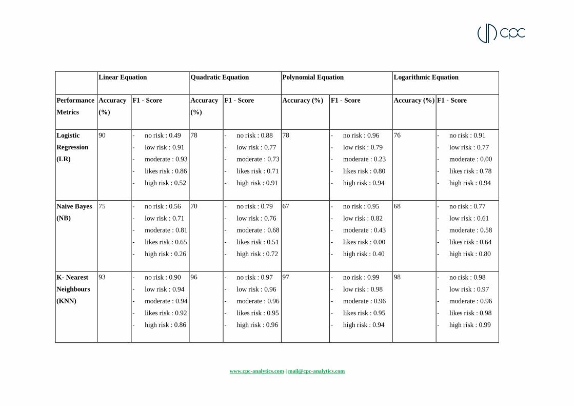
The accuracy of the prediction and the f1-scores of the classes need to be considered together
to select the best model for the dataset. The results (for five models and four input equations)
have been summarized in the table below (Table 1).
www.cpc-analytics.com | [email protected]
Linear Equation Quadratic Equation Polynomial Equation Logarithmic Equation
Performance
Metrics
Accuracy
(%)
F1 - Score Accuracy
(%)
F1 - Score Accuracy (%) F1 - Score Accuracy (%) F1 - Score
Logistic
Regression
(LR)
90 - no risk : 0.49
- low risk : 0.91
- moderate : 0.93
- likes risk : 0.86
- high risk : 0.52
78 - no risk : 0.88
- low risk : 0.77
- moderate : 0.73
- likes risk : 0.71
- high risk : 0.91
78 - no risk : 0.96
- low risk : 0.79
- moderate : 0.23
- likes risk : 0.80
- high risk : 0.94
76 - no risk : 0.91
- low risk : 0.77
- moderate : 0.00
- likes risk : 0.78
- high risk : 0.94
Naive Bayes
(NB)
75 - no risk : 0.56
- low risk : 0.71
- moderate : 0.81
- likes risk : 0.65
- high risk : 0.26
70 - no risk : 0.79
- low risk : 0.76
- moderate : 0.68
- likes risk : 0.51
- high risk : 0.72
67 - no risk : 0.95
- low risk : 0.82
- moderate : 0.43
- likes risk : 0.00
- high risk : 0.40
68 - no risk : 0.77
- low risk : 0.61
- moderate : 0.58
- likes risk : 0.64
- high risk : 0.80
K- Nearest
Neighbours
(KNN)
93 - no risk : 0.90
- low risk : 0.94
- moderate : 0.94
- likes risk : 0.92
- high risk : 0.86
96 - no risk : 0.97
- low risk : 0.96
- moderate : 0.96
- likes risk : 0.95
- high risk : 0.96
97 - no risk : 0.99
- low risk : 0.98
- moderate : 0.96
- likes risk : 0.95
- high risk : 0.94
98 - no risk : 0.98
- low risk : 0.97
- moderate : 0.96
- likes risk : 0.98
- high risk : 0.99
www.cpc-analytics.com | [email protected]
Support
Vector
Machines
(SVM)
98 - no risk : 0.63
- low risk : 0.97
- moderate : 0.99
- likes risk : 0.99
- high risk : 0.94
93 - no risk : 0.94
- low risk : 0.92
- moderate : 0.93
- likes risk : 0.93
- high risk : 0.94
96 - no risk : 0.96
- low risk : 0.95
- moderate : 0.95
- likes risk : 0.95
- high risk : 0.95
92 - no risk : 0.92
- low risk : 0.89
- moderate : 0.87
- likes risk : 0.94
- high risk : 0.96
Decision
Trees (DT)
89 - no risk : 0.81
- low risk : 0.89
- moderate : 0.90
- likes risk : 0.88
- high risk : 0.81
96 - no risk : 0.97
- low risk : 0.95
- moderate : 0.95
- likes risk : 0.95
- high risk : 0.95
98 - no risk : 0.99
- low risk : 0.98
- moderate : 0.97
- likes risk : 0.95
- high risk : 0.94
99 - no risk : 0.99
- low risk : 0.99
- moderate : 0.99
- likes risk : 0.99
- high risk : 0.99
Best Model K - Nearest Neighbours K - Nearest Neighbours Decision Tree Decision Tree
Explanatio
n
K - Nearest Neighbours can generate a highly convoluted
decision boundary, points that are very close to each other can be
modelled very well using this method.
Decision trees are good at classifying non linearly separable data.
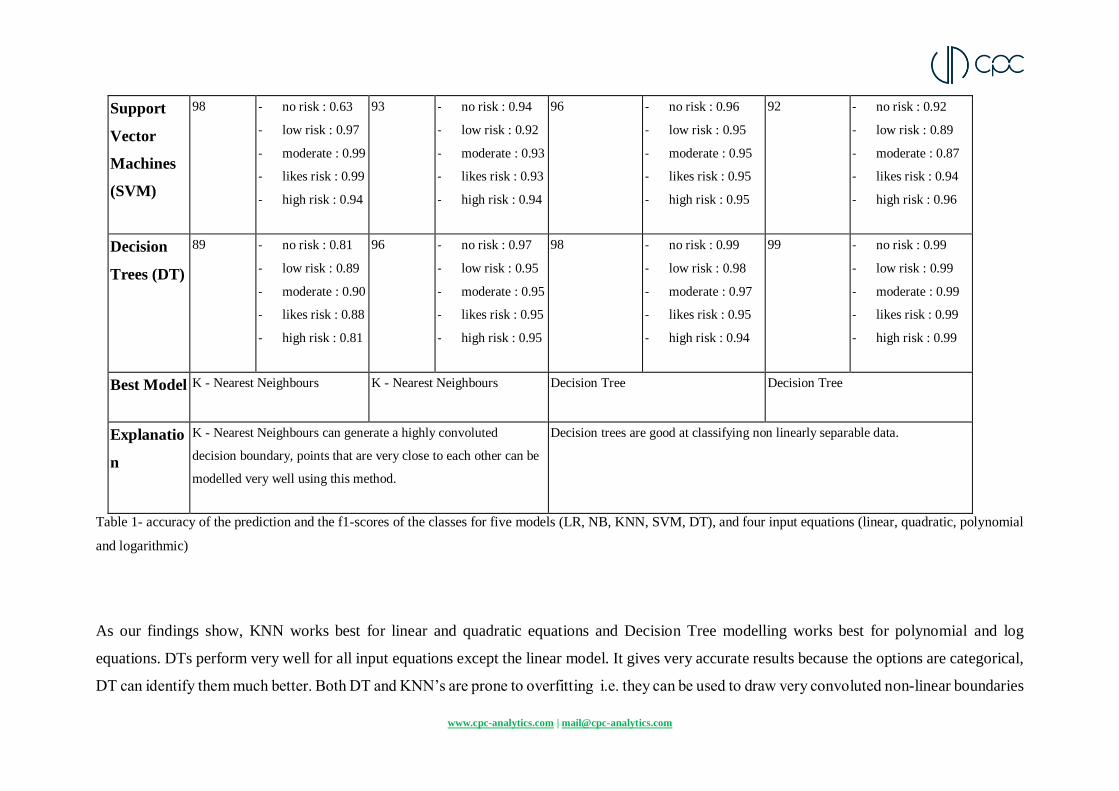
Table 1- accuracy of the prediction and the f1-scores of the classes for five models (LR, NB, KNN, SVM, DT), and four input equations (linear, quadratic, polynomial
and logarithmic)
As our findings show, KNN works best for linear and quadratic equations and Decision Tree modelling works best for polynomial and log
equations. DTs perform very well for all input equations except the linear model. It gives very accurate results because the options are categorical,
DT can identify them much better. Both DT and KNN’s are prone to overfitting i.e. they can be used to draw very convoluted non-linear boundaries

www.cpc-analytics.com | [email protected]
to seperate data points by repeatedly dividing data into specific classes or by creating very detailed neighbourhood clusters of data respectively.
The overfitting works in our favour in this case as we are looking for a closest representation of the dataset.
The findings also highlight why it is not sufficient to consider only the accuracy. Take the example of SVM on a linear equation. It gives a high
accuracy of 98%, higher than the KNN model. However, the f1 score of the no-risk class is only 0.63. This indicates that the SVM model can
make very good predictions for other classes, but fails to do it in the no-risk class.
All models would run on the input-output dataset given by the firm, and the model that gives the highest accuracy will be used to power the three
explanations. The accuracy and f1-scores will be reported to the regulator.

www.cpc-analytics.com | [email protected]
Part 2- Feature importance scores
Feature importance scores are part of the global explanations and have been found using the
SHAP values. They have been represented using SHAP plots. They tell how much each feature
(question) contributes to the ADS risk categorization process. Here, we report three importance
scores- the feature importance, the class-wise feature importance, and the class and category
wise feature importance.
Feature importance-
Figure 1- Global explanations
From the plot above we can gather that ‘Age’ is the most important feature in the model
contributing the most to all the categories which is positive as reflects the way we designed our
polynomial dataset. This allows the evaluator to understand the inner workings of the risk
profiling process and debug the algorithm used. The feature importances are useful but we will
benefit by going even deeper into understanding features and their behaviour for each class.
Class and category wise feature importance
The plots below cover the effect of each feature as well as show the importance of the features
in each category (risk class). The plots below have features on the y axis ordered based on their

www.cpc-analytics.com | [email protected]
importance and shapely values on the x axis. The colour represents the magnitude of each
feature. A sample of points are taken as representation and they are scattered to show a general
distribution of the data points.
Figure 2- Global explanation for each category.
A strikingly obvious trend can be seen in ‘Age’ where we can see high values of the feature go
from contributing highly positively to the high risk class to contributing negatively in the
low/no risk class. The second most important feature ‘Dependents’ is very important in the
extreme classes but shows no specific trend in the other classes. High values of annual income
and stability contribute negatively in low risk taking behaviour of individuals. Basically with
www.cpc-analytics.com | [email protected]
these plots we can see the general trends of the data points in the dataset and the model. In this
case they can correctly model and communicate the assumptions taken by us while generating
the dataset which will be an invaluable insight in cases where the assumptions are not available.
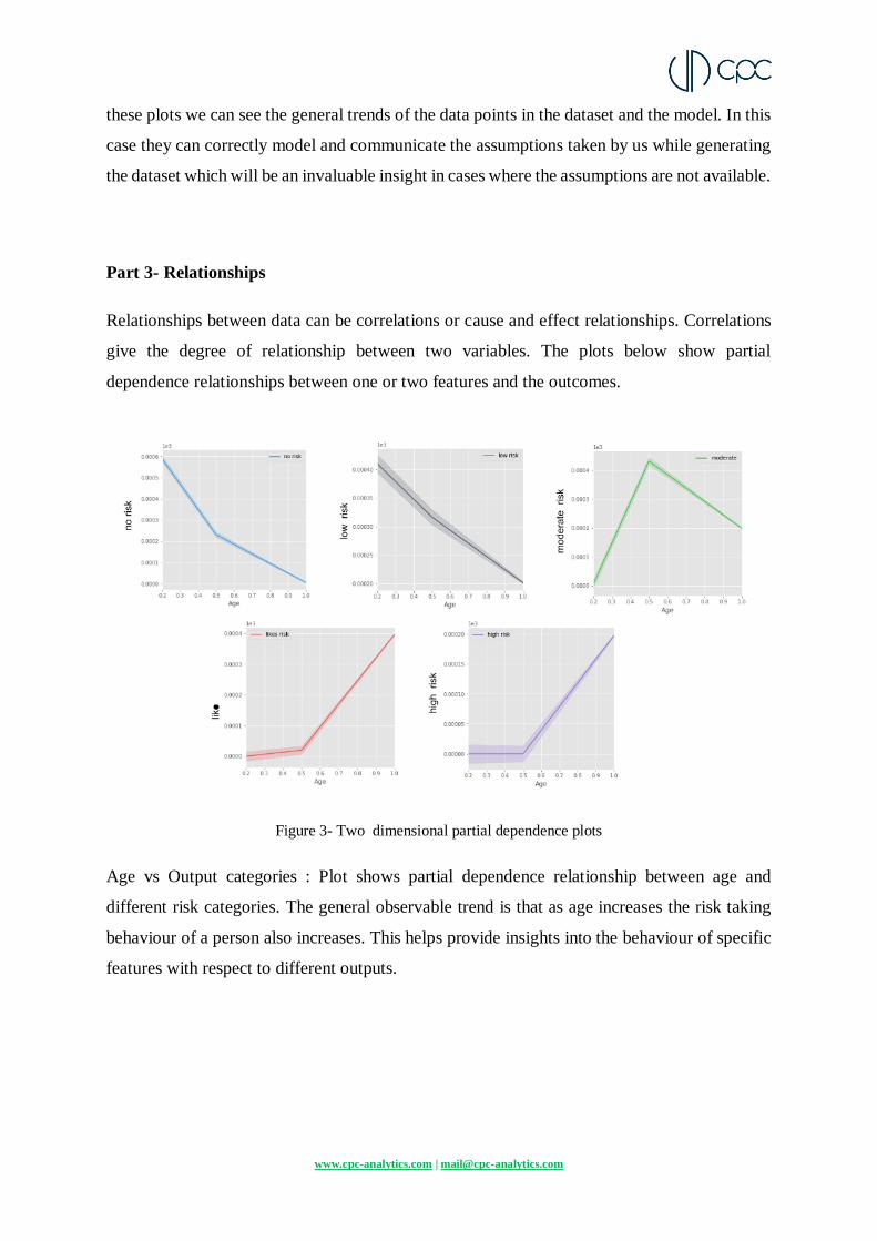
Part 3- Relationships
Relationships between data can be correlations or cause and effect relationships. Correlations
give the degree of relationship between two variables. The plots below show partial
dependence relationships between one or two features and the outcomes.
Figure 3- Two dimensional partial dependence plots
Age vs Output categories : Plot shows partial dependence relationship between age and
different risk categories. The general observable trend is that as age increases the risk taking
behaviour of a person also increases. This helps provide insights into the behaviour of specific
features with respect to different outputs.
www.cpc-analytics.com | [email protected]
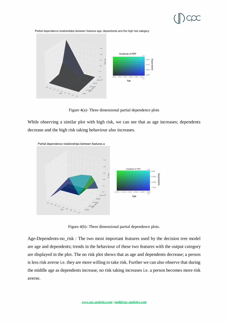
Figure 4(a)- Three dimensional partial dependence plots
While observing a similar plot with high risk, we can see that as age increases; dependents
decrease and the high risk taking behaviour also increases.
Figure 4(b)- Three dimensional partial dependence plots.
Age-Dependents-no_risk : The two most important features used by the decision tree model
are age and dependents; trends in the behaviour of these two features with the output category
are displayed in the plot. The no risk plot shows that as age and dependents decrease; a person
is less risk averse i.e. they are more willing to take risk. Further we can also observe that during
the middle age as dependents increase, no risk taking increases i.e. a person becomes more risk
averse.
www.cpc-analytics.com | [email protected]
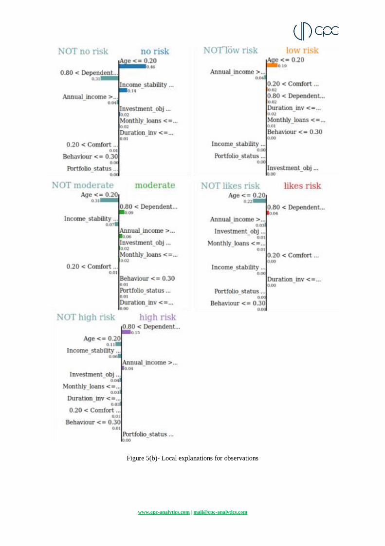
Part 4- Local explanations
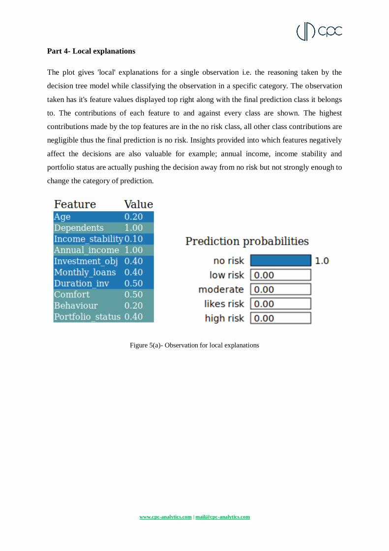
The plot gives 'local' explanations for a single observation i.e. the reasoning taken by the
decision tree model while classifying the observation in a specific category. The observation
taken has it's feature values displayed top right along with the final prediction class it belongs
to. The contributions of each feature to and against every class are shown. The highest
contributions made by the top features are in the no risk class, all other class contributions are
negligible thus the final prediction is no risk. Insights provided into which features negatively
affect the decisions are also valuable for example; annual income, income stability and
portfolio status are actually pushing the decision away from no risk but not strongly enough to
change the category of prediction.
Figure 5(a)- Observation for local explanations

www.cpc-analytics.com | [email protected]
Conclusion
We work ground up, trying to understand the scope and limitations of enforcing regulations on
technology by engaging with the technical challenges that it poses. We have survey various
methods to select a handful of tools that best explain the ADS. Based on this, we adopted two
global and one local explanation method using which, regulators can understand how each
question contributes to the output, how they relate to each other and conduct spot checks. The
methods used are able to model the dataset with high degree of accuracy. The methods have
been tested using various input conditions to ensure its reliability.
Revisiting the SEBI rules for automated tools in investment advisory, our study has proposed
an approach to operationalize a few regulations. This includes (1) providing users a meaningful
explanation of how the tool works and the outputs it generates; (2) subjecting the tool to a
comprehensive system audit and inspection. Indirectly, the explanations provided can be used
by the regulator to infer if (3) the tool used acts in the best interest of the client without any
unintended machine bias.
Thus, our approach has the potential to enhance the technical capabilities of capital markets
regulator without the need for in-house computer science expertise. Considerable work and
research would be required to create a comprehensive tool capable of operationalizing all
regulations.
Discussion and way forward
With technology permeating various aspects of public life, it needs to comply with the
standards set by law. However, designing and implementing regulations without knowledge of
how an algorithmic system works and what its externalities are would prove to be ineffective.
To formulate regulations that work, they need to be informed by the technical and operational
limitations. This is especially true for the case of ADS, where there are glaring problems and
yet there is a struggle to enforce concepts like fairness, accountability and transparency. As
(Goodman & Flaxman, 2017) point out the GDPR acknowledges that the few if any decisions
made by algorithms are purely ''technical'', that the ethical issues posed by them require rare
coordination between 'technical and philosophical resources’. Hence, we need dialogue
between technologist and regulators and they need to design safeguards together by pooling
their domain knowledge.

www.cpc-analytics.com | [email protected]
One way to achieve this is by creating regulatory sandboxes. Sandboxes act as test beds where
experiments can happen in a controlled environment. They are initiated by regulators for live
testing innovations of private firms in an environment that is under the regulators supervision
(Jenik & Lauer, 2017). It can provide a space for dialogue and developing regulatory
frameworks for the speed at which technological innovation happens, in a way that “doesn’t
smother the fintech sector with rules, but also doesn’t diminish consumer protection” (BBVA,
2017). This method would help build collaborative regulations and also open up the dialogue
of building in explainability by design in ADS early on in the process.
Future work needs to be on the regulatory and technical front. On the regulatory front, we need
to work with the regulators to understand the grasp-ability of various explanation methods.
Appropriate explanations also need to be extended to the user.
On the technical front, our work can be expanded to include increasingly more complex
situations. A standardized and robust documentation process for algorithms also needs to be
initiated to maintain accountability and makes it easier to audit the system.
Appendix
Appendix 1- Definitions and key terms
1. Feature- A feature is a measurable property of the object you’re trying to analyze. In
datasets, features appear as columns1.
1 https://www.datarobot.com/wiki/feature/
User Question 1-
age
Question 2-
salary/month
... Output- risk
category
User Profile 1 24 100,000 … High risk
User Profile 2 55 120,000 … Medium risk
User profile 3 36 75,000 … Low risk
.. .. … …
User profile n 42 50,000 … No risk
features
categories
classes
Sample of
user profiles-each row
represents one user
x

www.cpc-analytics.com | [email protected]
2. Accuracy- Accuracy gives the percentage of correctly predicted samples out of all the
available samples. Accuracy is not always the right metric to consider in imbalanced
class problems; in the risk dataset class 2 has the most samples, greatly outnumbering
samples in class 1 and 5. This could mean that even if most samples are incorrectly
labelled as belonging to class 2 then the accuracy would still be relatively high giving
us an incorrect understanding of the models working. Just considering the accuracy, the
most accurate classifier is the decision tree, closely followed by knn and svm who
supersede the logistic regression and naive bayes classifiers.
3. Recall- the ability of a model to find all the relevant samples. This gives the number of
true positive samples by the sum of true positive and false negative samples. True
positive samples are the samples correctly predicted as true by the model and false
negatives are data points the model identifies as negative that actually are positive (for
example points that belong to class 2 that are predicted as not belonging to class 2).
For example, in the performance metrics for logistic regression we find that the
performance is thrown off by class moderate/medium -risk takers, this is most probably
because the class has too many samples in the training data causing it to overfit(logistic
regression is prone to overfitting). Comparatively, except naive bayes all other
classifiers show consistently high recall values.
4. Precision- it is defined as the number of true positives divided by the number of true
positives plus the number of false positives. False positives are cases the model
incorrectly labels as positive that are actually negative, or in our example, individuals
the model classifies as class 2 that are not. While recall expresses the ability to find all
relevant instances in a dataset, precision expresses the proportion of the data points our
model says was relevant actually were relevant.
5. F1 score- Sometimes trying to increase precision can decrease recall and vice versa, an
optimal way to combine precision and recall into one metric is by using their harmonic
mean also called the F1-Score.
F1 = 2* (precision*recall)/(precision + recall)
www.cpc-analytics.com | [email protected]
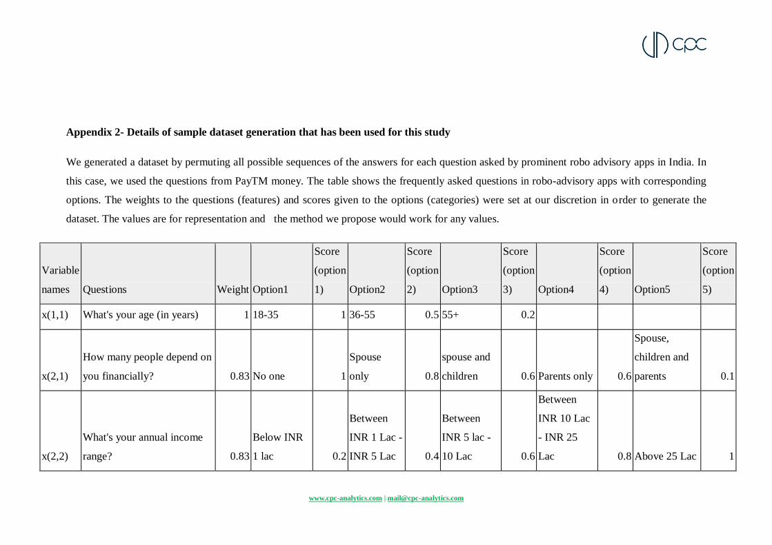
Appendix 2- Details of sample dataset generation that has been used for this study
We generated a dataset by permuting all possible sequences of the answers for each question asked by prominent robo advisory apps in India. In
this case, we used the questions from PayTM money. The table shows the frequently asked questions in robo-advisory apps with corresponding
options. The weights to the questions (features) and scores given to the options (categories) were set at our discretion in order to generate the
dataset. The values are for representation and the method we propose would work for any values.
Variable
names Questions Weight Option1
Score
(option
1) Option2
Score
(option
2) Option3
Score
(option
3) Option4
Score
(option
4) Option5
Score
(option
5)
x(1,1) What's your age (in years) 1 18-35 1 36-55 0.5 55+ 0.2
x(2,1)
How many people depend on
you financially? 0.83 No one 1
Spouse
only 0.8
spouse and
children 0.6 Parents only 0.6
Spouse,
children and
parents 0.1
x(2,2)
What's your annual income
range? 0.83
Below INR
1 lac 0.2
Between
INR 1 Lac -
INR 5 Lac 0.4
Between
INR 5 lac -
10 Lac 0.6
Between
INR 10 Lac
- INR 25
Lac 0.8 Above 25 Lac 1

www.cpc-analytics.com | [email protected]
x(3,1)
What % of your monthly
income do you pay in
outstanding loans, EMI etc? 0.65 None 1
Up to 20%
of income 0.8
20-30%
income 0.6
30-40% of
income 0.4
50% or above
of income 0.2
x(3,2)
Please select the stability of
your income 0.65
Very low
stability 0.1
Low
stability 0.3
Moderate
Stability 0.6
High
Stability 1
Very high
stability 1
x(4,1)
Where is most of your
current portfolio parked? 0.5
Savings and
fixed
deposits 0.4 Bonds/debt 0.6
Mutual
Funds 0.5
Real Estate
or Gold 0.4 Stock Market 0.8
x(5,1)
What's your primary
investment objective? 0.8
retirement
planning 0.65
Monthly
Income 0.6 Tax Saving 0.4
Capital
Preservation 0.5
Wealth
Creation 1
x(5,2)
How long do you plan to stay
invested? 0.8
Less than 1
year 0.5 1 to 3 years 0.8 3 to 5 years 0.65 5 to 10 years 0.6
more than 10
years 0.7
x(6,1)
To achieve high returns, you
are comfortable with high
risk investments 0.7
Strongly
agree 1 Agree 0.9 Neutral 0.5 Disagree 0.2
Strongly
disagree 0.1
x(6,2)
If you lose 20% of your
invested value one month
after investment, you will 0.65
Sell and
preserve
cash 0.2
Sell and
move cash
to fixed
deposits or
liquid fund 0.3
Wait till
market
recovers and
then sell 0.5
Keep
investments
as they are 0.8 Invest more 1

www.cpc-analytics.com | [email protected]
Table- Frequently asked questions in robo-advisory apps with corresponding options. The weights to the questions (features) and scores given to
the options (categories) were set a our discretion in order to generate the dataset. The values are for representation and the method would work
for any set values.
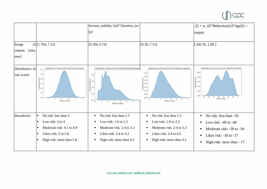
Types of
Equations
Linear Equation Polynomial Equation Quadratic Equation Logarithmic Equation
Equations w_11*Age + w_21*Dependents +
w_22*Annual_Income +
w_31*Monthly_loans +
w_32*Income_stability +
w_41*Portfolio_status +
w_51*Investment_obj +
w_52*Duration_inv +
w_61*Comfort + w_62*Behaviour
= output
w_11*Age + w_21*Dependents +
w_22* Annual_Income [k]*Age +
w_31* Monthly_loans[l]
*Age*Dependents + w_32*
Income_stability [m] + w_41*
x_41[n]* Age* Dependents
*Duration_inv[o] + w_51*
Investment_obj [o]* Age*
Dependents * Duration_inv [p] +
w_52* Duration_inv [p]*
Investment_obj [o]* Age*
Dependents + w_61* Comfort
[q]*Age*Dependents + w_62*
Behaviour [r]*Age*Dependents*
w_11*(Age**3) + w_21*Age*
(Dependents **2) + w_22*Age*
Annual_Income [k] + w_31*(
Monthly_loans [l]**2) + w_32*(
Income_stability [m]**3) +
w_41*Dependents*Portfolio_status[
n] + w_51*( Investment_obj
[o]**2)* Monthly_loans [l] + w_52*
Duration_inv[p]*Dependents +
w_61* Monthly_loans [l]* Comfort
[q] + w_62* Behaviour [r]*
Dependents
w_11*3*math.log(Age,3) +
w_21*2*math.log(Age[i]*
Dependents[j], 2) + w_22*3*
math.log( Age[i]* Annual_Income
[k],2) + w_31*3* math.log(Age[i]*
Monthly_loans[l], 2) + w_32*3*
math.log(Age[i]*Income_stability[m],
2) + w_41*Portfolio_status[n] +
w_51*3* math.log( Age[i]*
Income_stability[m]*
Investment_obj[o], 2) + w_52*
Duration_inv[p]* Behaviour [r] +
w_61*2* math.log(Comfort [q]*Age[i]
www.cpc-analytics.com | [email protected]
Income_stability [m]* Duration_inv
[p]
,2) + w_62*Behaviour[r]*Age[i] =
output
Range of
outputs [min,
max]
[1.764, 7.15] [0.394, 6.74] [0.18, 7.15] [-69.70, 1.69 ]
Distribution of
risk scores
Boundaries No risk: less than 3
Low risk: 3 to 4
Moderate risk: 4.1 to 4.9
Likes risk: 5 to 5.8
High risk: more than 5.8
No risk: less than 1.5
Low risk: 1.6 to 2.3
Moderate risk: 2.4 to 3.3
Likes risk: 3.4 to 4.3
High risk: more than 4.3
No risk: less than 1.5
Low risk: 1.6 to 2.3
Moderate risk: 2.4 to 3.3
Likes risk: 3.4 to 4.3
High risk: more than 4.3
No risk: less than -50
Low risk: -49 to -40
Moderate risk: -39 to -30
Likes risk: -30 to -17
High risk: more than - 17
www.cpc-analytics.com | [email protected]
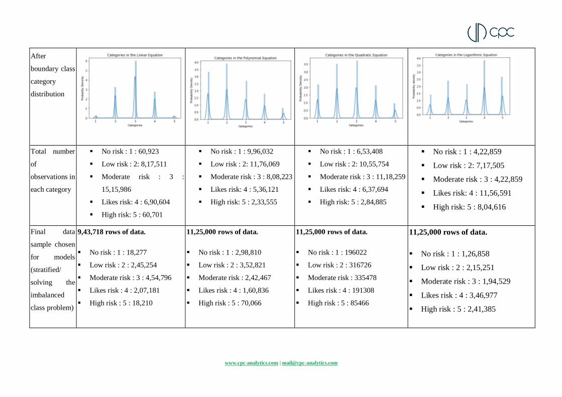
After
boundary class
category
distribution
Total number
of
observations in
each category
No risk : 1 : 60,923
Low risk : 2: 8,17,511
Moderate risk : 3 :
15,15,986
Likes risk: 4 : 6,90,604
High risk: 5 : 60,701
No risk : 1 : 9,96,032
Low risk : 2: 11,76,069
Moderate risk : 3 : 8,08,223
Likes risk: 4 : 5,36,121
High risk: 5 : 2,33,555
No risk : 1 : 6,53,408
Low risk : 2: 10,55,754
Moderate risk : 3 : 11,18,259
Likes risk: 4 : 6,37,694
High risk: 5 : 2,84,885
No risk : 1 : 4,22,859
Low risk : 2: 7,17,505
Moderate risk : 3 : 4,22,859
Likes risk: 4 : 11,56,591
High risk: 5 : 8,04,616
Final data
sample chosen
for models
(stratified/
solving the
imbalanced
class problem)
9,43,718 rows of data.
No risk : 1 : 18,277
Low risk : 2 : 2,45,254
Moderate risk : 3 : 4,54,796
Likes risk : 4 : 2,07,181
High risk : 5 : 18,210
11,25,000 rows of data.
No risk : 1 : 2,98,810
Low risk : 2 : 3,52,821
Moderate risk : 2,42,467
Likes risk : 4 : 1,60,836
High risk : 5 : 70,066
11,25,000 rows of data.
No risk : 1 : 196022
Low risk : 2 : 316726
Moderate risk : 335478
Likes risk : 4 : 191308
High risk : 5 : 85466
11,25,000 rows of data.
No risk : 1 : 1,26,858
Low risk : 2 : 2,15,251
Moderate risk : 3 : 1,94,529
Likes risk : 4 : 3,46,977
High risk : 5 : 2,41,385
www.cpc-analytics.com | [email protected]
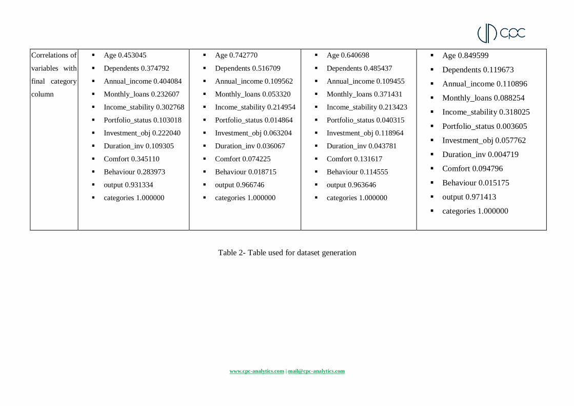
Correlations of
variables with
final category
column
Age 0.453045
Dependents 0.374792
Annual_income 0.404084
Monthly_loans 0.232607
Income_stability 0.302768
Portfolio_status 0.103018
Investment_obj 0.222040
Duration_inv 0.109305
Comfort 0.345110
Behaviour 0.283973
output 0.931334
categories 1.000000
Age 0.742770
Dependents 0.516709
Annual_income 0.109562
Monthly_loans 0.053320
Income_stability 0.214954
Portfolio_status 0.014864
Investment_obj 0.063204
Duration_inv 0.036067
Comfort 0.074225
Behaviour 0.018715
output 0.966746
categories 1.000000
Age 0.640698
Dependents 0.485437
Annual_income 0.109455
Monthly_loans 0.371431
Income_stability 0.213423
Portfolio_status 0.040315
Investment_obj 0.118964
Duration_inv 0.043781
Comfort 0.131617
Behaviour 0.114555
output 0.963646
categories 1.000000
Age 0.849599
Dependents 0.119673
Annual_income 0.110896
Monthly_loans 0.088254
Income_stability 0.318025
Portfolio_status 0.003605
Investment_obj 0.057762
Duration_inv 0.004719
Comfort 0.094796
Behaviour 0.015175
output 0.971413
categories 1.000000
Table 2- Table used for dataset generation

www.cpc-analytics.com | [email protected]
Appendix 3- Explaining the machine learning models
Logistic Regression
Logistic Regression is a commonly used statistical method for analysing and predicting data
with one or more independent variables and one binary dependent variable; for example spam
or not spam email classifiers, benign or malignant tumour detection. A logistic regression
classifier tries to fit data according to a linear hypothesis function such as Y= W(i)x(i) + B
(Similar to a line equation) where Y is the dependent variable, X represents independent
variables from 1 to n, B gives an error bias (negligible) and W is the weight assigned to each
variable. W is an important value as it tells us the individual contributions of variables in
determining Y, our target.
The independent variable is always binary, in our case there will be five logistic regression
classifiers with their independent variables as 1 (Low Risk) or Not 1 (Not Low Risk), 2 or Not
2 and so forth till case 5 (High Risk). This format of multiclass classification is called one vs
rest, the input sample is passed through all the classifiers and probability of the sample
belonging to classes 1 to 5 is calculated and the highest probability class wins.
The interpretation of weights in logistic regression is dependent on the probability of class
classification, the weighted sum is transformed by the logistic function to a probability.
Therefore the interpretation equation is:
Equation 3(a)- Log odds of logistic regression
The log function calculates the odds of an event occurring.
Equation 3(b)- Log odds of logistic regression

www.cpc-analytics.com | [email protected]
Logistic regression is used over linear regression as completely linear model does not output
probabilities, but it treats the classes as numbers (0 and 1) and fits the best hyperplane (for a
single feature, it is a line) that minimizes the distances between the points and the hyperplane.
So it simply interpolates between the points, and you cannot interpret it as probabilities. A
linear model also extrapolates and gives you values below zero and above one. Logistic
regression is also widely used, interpretable and fits our use case relatively well.
Support Vector Machine (SVM) Classifier
A support vector machine finds an equation of a hyper-plane that separates two or more classes
in a multidimensional space; for example if we consider a two dimensional space this
“hyperplane” will become a line dividing the plane on which the data lies into two separate
classes. If the data is not linearly separable i.e. there is no clear line separating the classes (This
happens in many cases imagine two classes in the data forming concentric circles ) then data
can be transformed onto a different plane (say we view the concentric circles from z axis ) it
becomes a linearly separable problem again ( Imagine the points in the circle having different
depth ), after separating we can transform it back to the original plane : this is done using a
kernel function in SVM.
Support vector machines have become wildly popular due to their robust efficiency and high
accuracy despite requiring very few samples to train. They have disadvantages especially when
it comes to time and space complexity but the SVM algorithm along with it’s variations are
being used commercially in face detection, protein fold predictions find some example
SVM for multiclass classification trains n*(n-1)/2 classifiers, where n is the number of classes
in the problem. Therefore for our problem there will be 10 different classifiers each will choose
permutations of classes as the binary dependent variable(Y) i.e. 1 or 2, 2 or 3, 1 or 4 and all
others. During this each classifier predicts one class instead of probabilities for each
Interpreting the above is quite difficult, the benefit of a linear model was that the weights /
parameters of the model could be interpreted as the importance of the features. Well we can’t
do that now, once we engineer a high or infinite dimensional feature set, the weights of the
model implicitly correspond to the high dimensional space which isn’t useful in aiding our
understanding of SVM’s. What we can do is fit a logistic regression model which estimates the
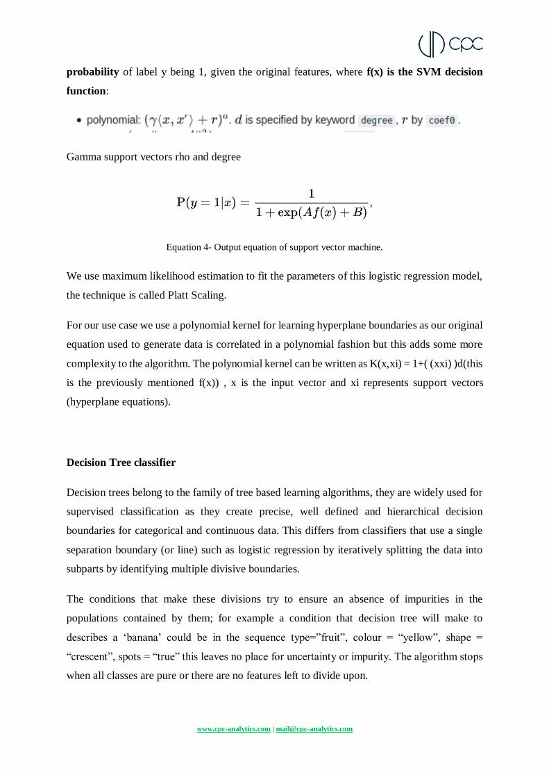
www.cpc-analytics.com | [email protected]
probability of label y being 1, given the original features, where f(x) is the SVM decision
function:
Gamma support vectors rho and degree
Equation 4- Output equation of support vector machine.
We use maximum likelihood estimation to fit the parameters of this logistic regression model,
the technique is called Platt Scaling.
For our use case we use a polynomial kernel for learning hyperplane boundaries as our original
equation used to generate data is correlated in a polynomial fashion but this adds some more
complexity to the algorithm. The polynomial kernel can be written as K(x,xi) = 1+( (xxi) )d(this
is the previously mentioned f(x)) , x is the input vector and xi represents support vectors
(hyperplane equations).
Decision Tree classifier
Decision trees belong to the family of tree based learning algorithms, they are widely used for
supervised classification as they create precise, well defined and hierarchical decision
boundaries for categorical and continuous data. This differs from classifiers that use a single
separation boundary (or line) such as logistic regression by iteratively splitting the data into
subparts by identifying multiple divisive boundaries.
The conditions that make these divisions try to ensure an absence of impurities in the
populations contained by them; for example a condition that decision tree will make to
describes a ‘banana’ could be in the sequence type=”fruit”, colour = “yellow”, shape =
“crescent”, spots = “true” this leaves no place for uncertainty or impurity. The algorithm stops
when all classes are pure or there are no features left to divide upon.
www.cpc-analytics.com | [email protected]
Unfortunately such sharp dividing conditions are not always possible or may exceed certain
time and space limitations in real life. Therefore when a clear separation of classes is not
possible then we can have a stopping condition that tolerates some impurity (For example gini
impurity measures quality of such splits by calculating the probability of an incorrect
classification of a randomly picked datapoint).
The impurity itself can be calculated using a measure of randomness, entropy: H= -
p(x)log(p(x))or -plog(p) -qlog(q) where p =probability of success and q = prob of failure
Ideally H should be as small as possible.
For a dataset like ours with multiple features, deciding the splitting feature i.e. most important
dividing condition at each step is a complex task, this feature should reduce the impurity
through the split or one with gives the most information gain. Information gain at each node
is calculated by the lowest entropy generated nodes by the split.
Starting from the root node, you go to the next nodes and the edges tell you which subsets you
are looking at. Once you reach a leaf node, the node tells you the predicted outcome. All the
edges are connected by ‘AND’. For example: If feature x is [smaller/bigger] than threshold c
AND etc… then the predicted outcome is the mean value of y of the instances in that node.
Individual decisions made by the tree can also be explained by going down a particular path
based on the input given.
Decision trees can be used to explain the dataset by themselves.
Naïve Bayes
Naive Bayes classifiers are a family of classifiers that work on predicting future outcomes using
conditional probability, given a history of behaviour; for example given say a year long history
of weather forecasts with features such as humidity, rainfall, temperature a classifier from the
naive Bayes family can be trained and used to predict future weather conditions.
The Bayes algorithm works under a “naive” assumption that all the features are independent in
nature, in our case that means the naive Bayes classifier is going to assume that our variables
such as age, income are uncorrelated so finding probabilities can be thought of as a simple
counting calculation. This implies that the classifier won’t be a right fit for our case as we know

www.cpc-analytics.com | [email protected]
that the data was generated using many correlations (such as age will affect an individual's
income, behaviour etc..). Due to its simplicity it has found a place in many real world systems
such as credit scoring systems, weather prediction and many others so for the sake of
representing and explaining all classifiers we will try this one out as well.
If the naive Bayes classifier wants to calculate the probability of observing features f1 to fn,
given a class c (In our case c here, represents the risk class and f values represent all our
question-answer scores), then
Equation 5(a)- Naïve bayes output probability
This means that when Naive Bayes is used to classify a new example, the posterior probability
is much simpler to work with:
Equation 5(b)- Group conditional probability
But we have left p(fn | c) undefined i.e. the occurrence of a certain feature given a class which
means we haven’t taken the distribution of the features into account yet. Therefore for our case
we have used a gaussian naive Bayes classifier that simply assumes p (fn | c) is a gaussian
normal distribution, this works well for our data which is a normal distribution.
Then the formula for our low risk class used by the classifier will be something like:
P ( low-risk / Age, Income, Dependents ..) = P( low-risk / Age-category) * P(low-risk / Income-
category) etc/ P(Age) * P(income) etc
This will be calculated for all risk categories and the class with the highest probability is given
as the final prediction.
Naive Bayes is an interpretable model because of the independence assumption. It can be
interpreted on the modular level. The contribution made by each feature towards a specific
class prediction is clear, since we can interpret the conditional probability.

www.cpc-analytics.com | [email protected]
K-Nearest Neighbours (KNN)
Neighbours-based classification is a type of instance-based learning or non-generalizing
learning: it does not try to construct a general internal model, but simply stores instances of
the training data. K nearest neighbours is perhaps the simplest algorithm, a data point is
classified by a majority vote of its neighbours. The input is assigned the class most common
among its ‘k’ nearest neighbours, where ‘k’ is a small positive integer, the value of ‘k’ is chosen
depending on the data. KNN is very useful in applications that require searching for similar
items; such as recommender systems, bio-surveillance software, document retrieval systems
such as concept search which is used in many e-Discovery software packages.
These neighbours are decided using brute force techniques that calculate distance from the data
point of interest to all the other data points in the dataset, by using formulae like Euclidean
distance. This means that the time and space complexity of this operation is very high; for n
samples in d dimensions the time complexity will be O(d*n*n) which makes this algorithm too
slow to run on large datasets such as ours but we will still cover it as it would be useful to see
people and question-answers that could be grouped into one risk category.
Since KNN is an instance based algorithm there is no learned model, there are no parameters
to learn, so there is no interpretability on a modular level. There is a lack of global model
interpretability because the model is inherently local and there are no global weights or
structures explicitly learned.
To explain a prediction at a local level, we can always retrieve the k neighbours that were used
for the prediction. This is useful for our dataset as there will be thousands of neighbouring data
points but presenting those ‘k’ nearest points could be a very useful explanation for each
category.
Bibliography
Narayanan, A. (2016, June 27). Investor Business Daily. Retrieved October 2019, from
https://www.investors.com/etfs-and-funds/etfs/fund-industry-wakens-from-slumber-
to-take-on-digital-advice-upstarts/
www.cpc-analytics.com | [email protected]
Carey, T. (2019, September 24). Investopedia. Retrieved October 2019, from
https://www.investopedia.com/robo-advisors-2019-where-have-all-the-assets-gone-
4767826
Goodman, B., & Flaxman, S. (2017). European Union regulations on algorithmic decision-
making and a ‘‘right to explanation’’. Retrieved October 2019, from
https://ora.ox.ac.uk/catalog/uuid:593169ee-0457-4051-9337-
e007064cf67c/download_file?file_format=pdf&safe_filename=euregs.pdf&type_of_
work=Journal+article
EU GDPR. (2016). EU GDPR Chapter 3. Retrieved October 2019, from https://gdpr.eu/article-
22-automated-individual-decision-making/
Wachter, S., Mittelstadt, B., & Floridi, L. (2016, December 28). Why a Right to Explanation
of Automated Decision-Making Does Not Exist in the General Data Protection
Regulation. International Data Privacy Law 2017.
Shneiderman, B. (2017, May 30). Algorithmic Accountability. The Alan Turing Institute.
Citron, D. K., & Pasquale, F. A. (2014). The Scored Society: Due Process for Automated
Predictions. Washington Law Review, 89, 1-34.
Kapur, D., & Khosla, M. (2019). Regulation in India: Design, Capacity, Performance. Hart
Studies in Comparitive Public Law.
Padmanabhan, A., & Rastogi, A. (2019). Big Data. In D. Kapur, & M. Khosla, Regulation in
India: Design, Capacity, Performance (pp. 251-278). Hart Studies in Comparitive
Public Law.
Ciocca, P., & Biancotti, C. (2018, October 23). Data superpowers in the age of AI: A research
agenda. VOX CEPR Portal.
Thelisson, E., Padh, K., & Celis, E. L. (2017, July 15). Regulatory Mechanisms and Algorithms
towards Trust in AI/ML.
Cowls, J., King, T., Taddeo, M., & Floridi, L. (2019, May 15). Designing AI for Social Good:
Seven Essential Factors. SSRN
https://papers.ssrn.com/sol3/papers.cfm?abstract_id=3388669.
www.cpc-analytics.com | [email protected]
Rudin, C. (2019, May 13). Stop explaining black box machine learning models for high stakes
decisions and use interpretable models instead. Nature Machine Intelligence, 206-215.
IOSCO. (2014, July). Report on the IOSCO Social Media and Automation of Advice Tools
Surveys . Retrieved September 2019, from
https://www.iosco.org/library/pubdocs/pdf/IOSCOPD445.pdf
Kaya, O. (2017, August 10). Robo-advice – a true innovation in asset management. Retrieved
September 2019, from https://www.dbresearch.com/PROD/RPS_EN-
PROD/PROD0000000000449125/Robo-
advice_%E2%80%93_a_true_innovation_in_asset_managemen.pdf
Abraham, F., Schmukler, S. L., & Tessada, J. (2019, Febuary). Robo-Advisors: Investing
through Machines. Retrieved October 2019, from
http://documents.worldbank.org/curated/en/275041551196836758/text/Robo-
Advisors-Investing-through-Machines.txt
FINRA. (2016, March). Report on Digital Investment Advice. Retrieved September 2019, from
FINANCIAL INDUSTRY REGULATORY AUTHORITY:
https://www.finra.org/sites/default/files/digital-investment-advice-report.pdf
Dastin, J. (2018, October 10). Amazon scraps secret AI recruiting tool that showed bias against
women. (Reuters) Retrieved September 2019, from https://www.reuters.com/article/us-
amazon-com-jobs-automation-insight/amazon-scraps-secret-ai-recruiting-tool-that-
showed-bias-against-women-idUSKCN1MK08G
ProPublica. (2016, May 23). Machine Bias There’s software used across the country to predict
future criminals. And it’s biased against blacks. Retrieved September 2019, from
https://www.propublica.org/article/machine-bias-risk-assessments-in-criminal-
sentencing
Datta, A., Tschantz, M. C., & Datta, A. (2015, February 18). Automated Experiments on Ad
Privacy Settings. Proceedings on Privacy Enhancing Technologies , 92-112.
Costello, M., Hawdon, J., Ratliff, T., & Grantham, T. (2016, May). Who views online
extremism? individual attributes leading to exposure. Computers in Human Behavior.

www.cpc-analytics.com | [email protected]
Baer, D. (2019, November). The ‘Filter Bubble’ Explains Why Trump Won and You Didn’t See
It Coming. Retrieved October 2019, from The Cut:
https://www.thecut.com/2016/11/how-facebook-and-the-filter-bubble-pushed-trump-
to-victory.html
Obermeyer, Z., Powers, B., Vogeli, C., & Mullainathan, S. (2019, October 25). Dissecting
racial bias in an algorithm used to manage the health of populations. Science.
Kari, P. (2019, October 25). Healthcare algorithm used across America has dramatic racial
biases. Retrieved October 2019, from Guardian:
https://www.theguardian.com/society/2019/oct/25/healthcare-algorithm-racial-biases-
optum
Castelluccia , C., & Le Métayer, D. (March 2019). Understanding algorithmic decision-
making: Opportunities and challenges. Study, European Parliamentary Research
Services, Panel for the Future of Science and Technology.
Maurell, v. d. (2019). Embracing Robo Advisory looks promising or the longitivity of Financial
Advisors. Global Financial Markets Institute, New York.
Wired.com. (2019, November 19). The apple card didn't see gender and that's the problem.
Retrieved December 2019, from https://www.wired.com/story/the-apple-card-didnt-
see-genderand-thats-the-problem/
FAT ML. (n.d.). Principles for Accountable Algorithms and a Social Impact Statement for
Algorithms. Retrieved December 2019, from
https://www.fatml.org/resources/principles-for-accountable-algorithms
Philippe Bracke, A. D. (2019). Machine learning explainability in finance: an application to
default risk analysis. https://www.bankofengland.co.uk/-/media/boe/files/working-
paper/2019/machine-learning-explainability-in-finance-an-application-to-default-risk-
analysis.pdf, Bank of England.
Hall, P., & Gill, N. (2018). An Introduction to Machine Learning Interpretability. (N. Tache,
Ed.) O'Reilly.

www.cpc-analytics.com | [email protected]
BBVA. (2017, November 18). What is a regulatory sandbox? Retrieved December 2019, from
https://www.bbva.com/en/what-is-regulatory-sandbox/
Jenik, I., & Lauer, K. (2017). Regulatory Sandboxes and Financial Inclusion. CAGP.
https://www.cgap.org/sites/default/files/Working-Paper-Regulatory-Sandboxes-Oct-
2017.pdf.