Operational ocean models in the Adriatic Sea: a skill

Ocean Sci., 4, 61–71, 2008www.ocean-sci.net/4/61/2008/© Author(s) 2008. This work is licensedunder a Creative Commons License.

Ocean Science

Operational ocean models in the Adriatic Sea: a skill assessment

J. Chiggiato1,* and P. Oddo2

1Servizio IdroMeteorologico, ARPA Emilia Romagna, Viale Silvani 6, 40122 Bologna, Italy2Istituto Nazionale di Geofisica e Vulcanologia, Unita Funzionale di Climatologia Dinamica, via Aldo Moro 44, 40127Bologna, Italy* now at: CNR-ISMAR, Castello 1364, 30122 Venezia, Italy

Received: 30 November 2006 – Published in Ocean Sci. Discuss.: 21 December 2006Revised: 18 October 2007 – Accepted: 18 January 2008 – Published: 15 February 2008

Abstract. In the framework of the Mediterranean Fore-casting System (MFS) project, the performance of re-gional numerical ocean forecasting systems is assessedby means of model-model and model-data comparison.Three different operational systems considered in this studyare: the Adriatic REGional Model (AREG); the Adri-atic Regional Ocean Modelling System (AdriaROMS) andthe Mediterranean Forecasting System General CirculationModel (MFS-GCM). AREG and AdriaROMS are regionalimplementations (with some dedicated variations) of POMand ROMS, respectively, while MFS-GCM is an OPA basedsystem. The assessment is done through standard scores. Insitu and remote sensing data are used to evaluate the systemperformance. In particular, a set of CTD measurements col-lected in the whole western Adriatic during January 2006 andone year of satellite derived sea surface temperature measure-ments (SST) allow to asses a full three-dimensional pictureof the operational forecasting systems quality during January2006 and to draw some preliminary considerations on thetemporal fluctuation of scores estimated on surface quanti-ties between summer 2005 and summer 2006.

The regional systems share a negative bias in simulatedtemperature and salinity. Nonetheless, they outperform theMFS-GCM in the shallowest locations. Results on ampli-tude and phase errors are improved in areas shallower than50 m, while degraded in deeper locations, where major mod-els deficiencies are related to vertical mixing overestimation.In a basin-wide overview, the two regional models show dif-ferences in the local displacement of errors. In addition, inlocations where the regional models are mutually correlated,the aggregated mean squared error was found to be smaller,that is a useful outcome of having several operational sys-tems in the same region.

Correspondence to:P. Oddo([email protected])

1 Introduction

Ocean physical processes play a crucial role in governingmarine dynamics (acoustical, biological and sedimentolog-ical). Therefore, operational forecasting of physical oceanfields can greatly contribute to our understanding of the func-tioning of marine sub-systems, as well as providing an ef-ficient support tool for marine environmental management(Oddo et al., 2006; Robinson and Sellschopp, 2002). For sev-eral applications such as fisheries management, naval opera-tions, shipping, tourism, administration of marine resourcesand also for pure scientific purposes, high-resolution oceanforecasts are frequently required for limited regions (Onkenet al., 2005).

Focusing on characteristic scales, processes and dynam-ics of a limited area, allows devoting particular attentionto regionally specific numerical requirements (i.e. approxi-mations, parameterizations, resolution and numerical tech-niques). Currently, several numerical models exist based onthe same physical assumptions, and each single model showsits specific behaviour. Since model results derive from phys-ical laws warped by numerical discretisation techniques, thepossibility of having several numerical models implementedin the same area increases the confidence in model results.

In the framework of Mediterranean Forecasting Systemproject (MFS, Pinardi et al., 2003) a suite of numerical oceanmodels has been developed and implemented in the Mediter-ranean Sea. The MFS modelling system is composed of alarge-scale, coarse-resolution general circulation model cov-ering the entire Mediterranean Sea (MFS-GCM) and a num-ber of embedded high-resolution models in different regionalseas. In the operational chain the MFS-GCM produces anal-ysis/forecast for basin scale and provides initial and/or lateralboundary conditions for the regional models.

In this study the performance of the MFS modelling sys-tem in the Adriatic Sea is investigated. To our knowl-edge, two regional Operational Ocean Forecasting Systems

Published by Copernicus Publications on behalf of the European Geosciences Union.

brought to you by COREView metadata, citation and similar papers at core.ac.uk

provided by Directory of Open Access Journals

https://core.ac.uk/display/26899885?utm_source=pdf&utm_medium=banner&utm_campaign=pdf-decoration-v1

62 J. Chiggiato and P. Oddo: Operational ocean models in the Adriatic Sea

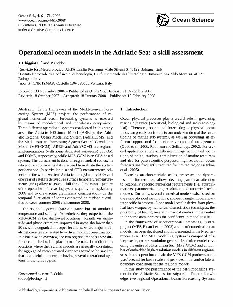
Fig. 1. Adriatic Sea coastline and bathymetry. Small circles rep-resent CTDs locations. Note that iso-contours of depth 20 m, 50 mand 200 m, shown in the plot, are the very same used in the group-ing done in Sect. 3. The grey thick line at 39 N represents AREGopen boundary, while the black thick line at roughly 40 N representsAdriaROMS open boundary.

(hereinafter OOFS) are currently producing daily or weeklyforecasts, published on free-access web sites, covering thewhole Adriatic Sea with full three-dimensional implemen-tation of the core ocean models: the Adriatic REGionalforecasting system (AREG) and the Adriatic ROMS (Adri-aROMS). The major aim of this work is to assess the per-formance of these two different regional OOFSs, eventuallyshowing potential advantages deriving from specific regionalimplementation and from having more OOFSs in the samearea. For completeness, the MFS-GCM is also included inthis analysis, even if to a lesser extent, as a proxy of therelative large vs. regional scale systems performance. Theanalysis is focused on the quality of the operational systems,i.e., the agreement between model results and independentobservations, therefore using the best available model output(best real-time estimates, including analyses). The relativeskill to provide accurate short term forecast is left to otherinvestigations.

The analysis is limited to temperature and salinity fieldsdue to data availability.

The operational ocean forecasting systems are presented inSect. 2. The comparisons between model results and in situobservations or remote sensing (AVHRR) data are presentedand discussed in Sects. 3 and 4, respectively. Concludingremarks are given in Sect. 5.

2 Operational ocean forecasting systems

In this section all the considered operational forecasting sys-tems for the comparison are briefly described. These systemsdiffer in many aspects, such as their operational suite, spa-tial discretisation, physical parameterizations, and numericalweather prediction model used for the surface boundary con-dition. The major differences between operational forecast-ing systems are summarized in Table 1 for enhanced read-ability.

2.1 AREG

The AREG model domain covers the entire Adriatic Seabasin and extends into the Ionian Sea (Fig. 1). The horizon-tal resolution is approximately 5 km, while, for the vertical,21 σ -coordinate levels are used. The model is based on thePrinceton Ocean Model, POM (Blumberg and Mellor, 1987)as implemented in the Adriatic Sea by Zavatarelli and Pinardi(2003). The current implementation makes use of an iterativeadvection scheme for tracers (Smolarkiewicz, 1984) imple-mented into POM following Sannino et al. (2002). Surfaceforcing functions are obtained via standard bulk formulae(Oddo et al., 2005) using European Centre for Medium-rangeWeather Forecast (ECMWF) operational fields and AREGsimulated sea surface temperature. A detailed description ofthe numerical model and forecasting system implementationcan be found in Oddo et al. (2005, 2006).

2.2 AdriaROMS

AdriaROMS is the operational ocean forecast system for theAdriatic Sea running at the Hydro-meteorological Service ofEmilia Romagna (ARPA-SIM). It is based on the RegionalOcean Modelling System (ROMS, detailed kernel descrip-tion is in Shchepetkin and McWilliams, 2005). This Adriaticconfiguration has a variable horizontal resolution, rangingfrom 3 km in the north Adriatic to∼10 km in the south, with20 s-coordinate levels for the vertical. A third order upstreamscheme is used for advection (Shchepetkin and McWilliams,1998); a Laplacian operator adds a weak grid-size depen-dent on horizontal diffusivity, while no horizontal viscosityis used. The Mellor and Yamada (1982) 2.5 scheme is usedfor the vertical mixing, and density Jacobian scheme withspline reconstruction of the vertical profiles is used for thepressure gradient (Shchepetkin and McWilliams, 2003). Themodel was initialized in September 2004 from MFS-GCMfields optimally interpolated onto AdriaROMS grid, then runin pre-operational configuration until June 2005 when thefirst forecasts were published on the web.

Surface forcing is provided by the Limited Area ModelItaly (LAMI, local implementation of the LM model, Step-peler et al., 2003), a non hydrostatic numerical weather pre-diction model with 7 km horizontal resolution providing tri-hourly shortwave radiation, 10 m wind, 2 m temperature,

Ocean Sci., 4, 61–71, 2008 www.ocean-sci.net/4/61/2008/

J. Chiggiato and P. Oddo: Operational ocean models in the Adriatic Sea 63

Table 1. Summary of some of the most relevant differences between the three operational forecasting systems.

OOFS MFS-GCM AREG AdriaROMS

Dataset Analysis (weekly) Hindcast (weekly) Sequential forecast(03:00–24:00)

Horizontal resolution 1/16◦ (∼7 km) 5 km Variable (3 km÷∼10 km)

Vertical Resolution 72 uneven z-coordinate 21 sigma coordinate 20 non linear s-coordinate

Output Daily averages Daily averages 3-hourly snapshots

Initialisation Summer 2004 Spring 2003 Fall 2004

Domain Mediterranean Sea Adriatic Sea Adriatic Sea

Meteorological forcing ECMWF analyses(1/2◦, 6-hourly)

ECMWF analyses(1/2◦, 6-hourly)

LAMI forecasts(7 km, 3-hourly)

Heat flux Computed w/ flux correc-tion (SST from AVHRR)

Computed w/out fluxcorrection

Computed w/out fluxcorrection

Fresh water flux Relaxation to climatologi-cal SSS

Fresh water flux as salinityflux, all rivers but Po are cli-matological.

Only river flux (as source ofmass and momentum); allrivers but Po are climato-logical

Data Assimilation ARGO XBT SLA (onlyXBT in the Adriatic region)

none none

Core Ocean Model OPA POM ROMS

relative humidity, total cloud cover, mean sea level pressureand precipitation. All of them are used to compute momen-tum and heat fluxes. Long wave radiation is estimated us-ing Berliand formula (Budyko, 1974), turbulent fluxes fol-lowing Fairall et al. (1996), while no evaporation precipita-tion flux was included (added in a later version). MFS-GCMdata are used at the open boundary to the south (see Fig. 1)with clamped boundary conditions with superimposed fourmajor tidal harmonics (S2, M2, O1, K1), from the workof Cushman-Roisin and Naimie (2002), following Flather(1976). Forty-eight rivers and springs are included as well,using monthly climatological values from Raicich (1996).Persistence of daily discharge measured one day backwardis used for the Po River.

2.3 MFS-GCM

The MFS-GCM (Tonani et al., 2008), based on the OPA code(Madec et al., 1998), covers the entire Mediterranean Seawith a horizontal resolution of 1/16 of degree and 72 un-evenly spaced z-coordinate levels on the vertical. The modelis forced at the surface with ECMWF analysis and forecastatmospheric fields. It uses a reduced order optimal interpo-lation assimilation scheme (SOFA; De Mey and Benkiran,2002; Demirov et al., 2003; Dobricic et al., 2007) to cor-rect the model solution using vertical profiles from XBT and

ARGO, and satellite data of sea level anomaly (Pinardi etal., 2003), as well as flux corrections (relaxation to climato-logical sea surface salinity and sea surface temperature fromAVHRR data). The ocean analysis-forecast consists of dailymean oceanographic fields computed for the entire Mediter-ranean basin. These fields are used in the two regional mod-els to prescribe lateral open boundary conditions.

2.4 Selection of the time series

Databases of OOFSs output used in this paper are hind-cast (AREG), forecast (AdriaROMS) and analysis (MFS-GCM). This choice followed from the OOFS operationalchains. AREG and MFS-GCM produce weekly 9-day fore-casts, thus combining a time series of weekly forecasts wouldalso include the “day-of-the-week-dependent” signal of fore-cast growing error in the quality assessment. Selecting hind-cast for AREG (analyses are not performed) and analyses forMFS-GCM allows building a time-series unaffected by thissignal. On the other hand, forecasts obtained by AdriaROMSare produced daily (and no hindcasts or analyses are avail-able) therefore a time series built using the first day of theforecast is the best dataset available. This approach is rea-sonable since it is the quality of the OOFS being assessed inthis work, instead of the performance throughout the forecastrange.

www.ocean-sci.net/4/61/2008/ Ocean Sci., 4, 61–71, 2008


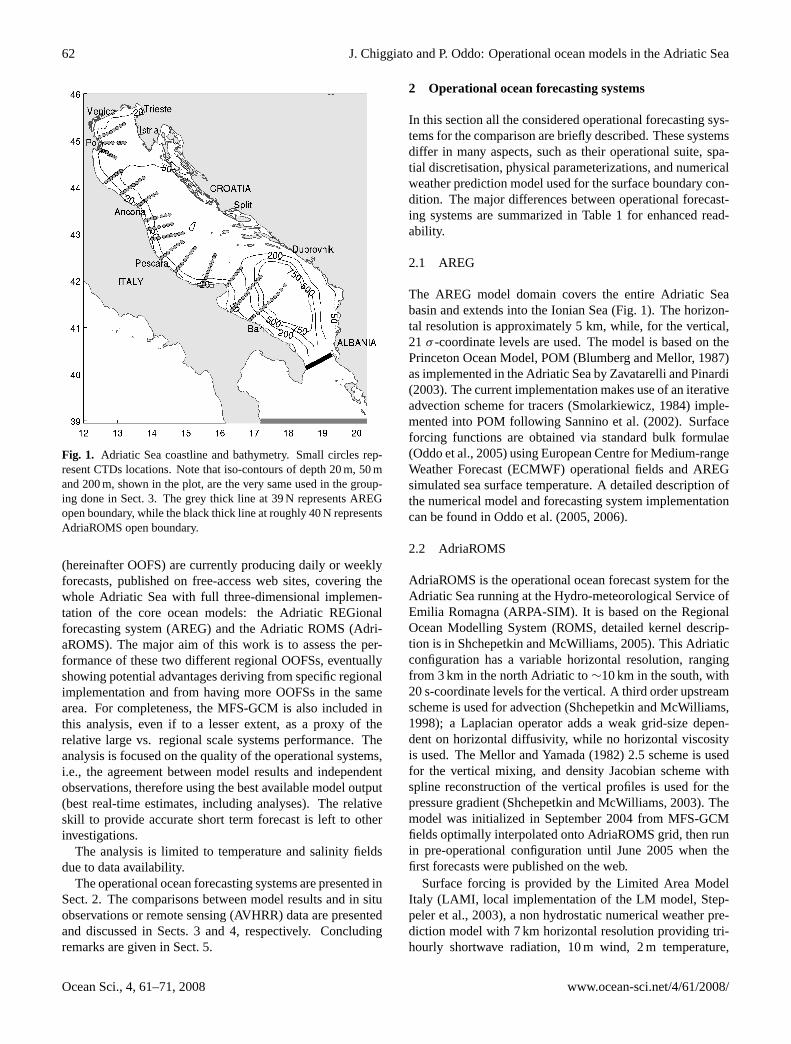
Fig. 2. Respectively from top to bottom: daily, basin averaged windstress magnitude, wind stress curl and heat fluxes filtered with a10-day running mean to enhance readability.

2.5 Diagnosed surface fluxes

Inter-comparison of the operational systems involves the rel-evant role of the atmospheric forcing; as given in Table 1,AREG and MFS-GCM are driven by a large-scale generalcirculation model (ECMWF), while AdriaROMS by a lim-ited area model (LAMI). Due to the complex orography sur-rounding the Adriatic Sea, a proper representation of thecoastal meteorology in that region is not trivial. Recent stud-ies (Signell et al., 2005) have shown that in atmospheric mod-els with coarse resolution (roughly larger than 10 km) windfields are generally underestimated in the Adriatic, especiallyin the northern sector. Concerning heat fluxes, while the sig-nal at the large scale may not necessarily be different usingcoarse or high resolution atmospheric models, some small-scale differences are expected due to the different physicsand orography implemented in the models themselves.

The time series of wind stress magnitude and curl areshown in Fig. 2. Note that the basin-averaged magnitude issimilar for both systems, while the wind stress curl showssimilar patterns (mostly cyclonic vorticity) but often differsin magnitude, specially in winter. AdriaROMS has generallylarger values due to steep gradients associated to limited areamodel small scale structures.

Major differences, even in the basin-averaged time series,are observed in the computation of surface heat fluxes. Froma climatological point of view, the Adriatic Sea is believedto loose heat at the surface, although with large inter-annualvariability and eventually years of heat gain (see Oddo etal., 2005 and citation therein). As seen in Fig. 2, AREGshows larger heat gain during summer, while AdriaROMSshows lesser heat loss during autumn-winter. On a shorttime scale, differences in the basin averaged between the twoOOFSs can be as high as 100–150 W/m2. In the consideredyear, AREG averaged heat flux is−14 W/m2, associated toa meridional heat flux incoming from the southern boundary,while AdriaROMS heat flux is +3 W/m2, with weak merid-ional heat flux outgoing through the southern boundary. Al-though AREG results seem more consistent with long termclimatology (Artegiani et al., 1997), it is not possible to as-sess which behaviour is actually correct, given the limitedobservational dataset at hand.

Surface fresh water fluxes are not considered here sincethey are not routinely stored in the AdriaROMS nor AREGarchive.

3 Comparison with in situ temperature and salinity

3.1 CTD data and methods

In January 2006, an extensive dataset of CTD measure-ments was collected during the cruise R/V URANIA in thewestern Adriatic Sea. This dataset (courtesy of CNR-ISACGruppo di Oceanografia da Satellite, Roma, IT) provided the



opportunity to assess a temporal snapshot of the ocean fore-casting systems performance operating in the Adriatic Sea.The dataset consists of 150 CTD casts organized along 15cross-shore sections (see Fig. 1), performed between 14 and27 January 2006. The full CTD dataset has been split intofour sub-categories, depending on the depth of the samplingpositions. The grouping was done to evaluate scores fromdifferent coastal to open sea regions .The rationale is thatregional forecasting systems are built to provide more accu-rate “information” on the coastal zones that may be roughlyrepresented in large-scale systems; therefore, it is desirableto understand if the regional systems actually have skills insuch areas.

The regions have been defined as follows:

1. Very shallow region (group G1): casts in depths not ex-ceeding 20 m.

2. Shallow region (G2): casts in depths between 20 and 50m.

3. Mid-depth region (G3): casts in depths between 50 and200 m.

4. Deep region (G4): casts in depths exceeding 200 m.

A first general overview of the performance was done bymeans of Mean Errors (ME) and Root Mean Square Error(RMSE). Scores are estimated interpolating model result intime and space on the CTD locations. Within each group allsquared errors have been aggregated over time and space (ina quasi-synoptic assumption) before taking the mean and theroot mean square.

Rating the relative performance compared to MFS-GCM,it was decided to estimate the Mean Squared Error SkillScore (hereinafter MSESS, see Appendix A) at each CTDsite and then to compute the number of significantly positive,significantly negative and not-significantly different valueswithin each group. Therefore, a larger number of positiveskill scores suggest a relatively better performance. Signifi-cance of the scores is estimated using the bootstrap techniquewith 1000 re-samples. Observations used in this assessmentwere not assimilated in the MFS-GCM.

3.2 Results

Results of the statistical assessment are summarized in Ta-ble 2. AdriaROMS shows negligible mean error in tem-perature in the two shallower groups, while temperaturesare lower than those observed at G3 and, in particular, atG4, where there is a bias throughout the full water column(ME∼RMSE). Given the depth at G4 (>200 m), and thetime-scale of the major regional processes, this is unlikelydue directly to surface forcing, but to the proximity of theopen boundary and to the heat content derived by the ini-tialization, since MFS-GCM itself is similarly biased in thatregion. AREG gives good accuracy for G1 and G4, while

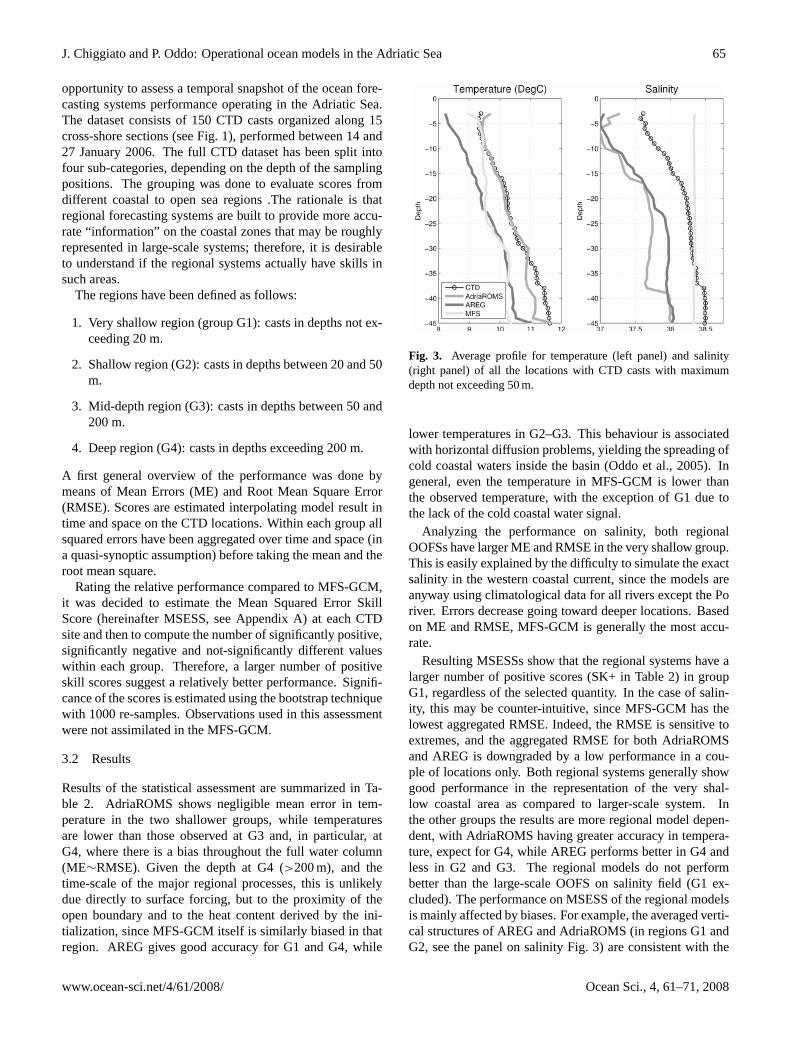
Fig. 3. Average profile for temperature (left panel) and salinity(right panel) of all the locations with CTD casts with maximumdepth not exceeding 50 m.

lower temperatures in G2–G3. This behaviour is associatedwith horizontal diffusion problems, yielding the spreading ofcold coastal waters inside the basin (Oddo et al., 2005). Ingeneral, even the temperature in MFS-GCM is lower thanthe observed temperature, with the exception of G1 due tothe lack of the cold coastal water signal.

Analyzing the performance on salinity, both regionalOOFSs have larger ME and RMSE in the very shallow group.This is easily explained by the difficulty to simulate the exactsalinity in the western coastal current, since the models areanyway using climatological data for all rivers except the Poriver. Errors decrease going toward deeper locations. Basedon ME and RMSE, MFS-GCM is generally the most accu-rate.

Resulting MSESSs show that the regional systems have alarger number of positive scores (SK+ in Table 2) in groupG1, regardless of the selected quantity. In the case of salin-ity, this may be counter-intuitive, since MFS-GCM has thelowest aggregated RMSE. Indeed, the RMSE is sensitive toextremes, and the aggregated RMSE for both AdriaROMSand AREG is downgraded by a low performance in a cou-ple of locations only. Both regional systems generally showgood performance in the representation of the very shal-low coastal area as compared to larger-scale system. Inthe other groups the results are more regional model depen-dent, with AdriaROMS having greater accuracy in tempera-ture, expect for G4, while AREG performs better in G4 andless in G2 and G3. The regional models do not performbetter than the large-scale OOFS on salinity field (G1 ex-cluded). The performance on MSESS of the regional modelsis mainly affected by biases. For example, the averaged verti-cal structures of AREG and AdriaROMS (in regions G1 andG2, see the panel on salinity Fig. 3) are consistent with the



Table 2. Mean error, root mean square error and mean square error skill scores in the four groups G1, G2, G3, G4, divided by the rangeof depth of the CTD locations. SK+, SK−, SK? mean, respectively, the number of profiles in which the skill score is significantly positive(regional system is best), negative (the large scale system is best) or not significantly different (neutral).

TEMP SALT

ME RMSE SK+ SK− SK? ME RMSE SK+ SK- SK?

AdriaROMS

G1 0–20 +0.09 1.03 16 4 1 −1.11 2.52 13 5 3G2 20–50 −0.06 0.94 26 18 3 −0.54 0.72 4 40 3G3 50–200 −0.73 0.98 30 26 2 −0.46 0.50 1 56 1G4 200-inf −1.05 1.09 1 22 0 −0.34 0.34 0 23 0

AREG

G1 0–20 −0.03 1.35 11 7 3 −0.75 1.97 11 7 3G2 20–50 −0.96 1.65 15 23 9 −0.48 0.85 12 32 3G3 50–200 −0.90 1.32 18 37 3 −0.58 0.66 2 54 2G4 200-inf −0.02 0.25 16 7 0 −0.28 0.28 14 9 0

MFS

G1 0–20 +1.13 1.97 +1.31 1.56G2 20–50 −0.73 1.49 +0.11 0.54G3 50–200 −0.76 1.25 −0.30 0.32G4 200-inf −0.54 0.59 −0.31 0.31

observations, giving good results on linear association andamplitude error, but biases eventually downgrade the perfor-mance on skill scores compared to MFS-GCM. It becamethen necessary to investigate further the actual skill of the re-gional OOFSs with other statistics, i.e., looking at amplitudeand phase errors and not just at MSE. Results of these statis-tics are shown in Fig. 4a (grouping G1 and G2 together) andFig. 4b (G3+G4). In G1+G2, the correlations in both AREGand AdriaROMS are similar and reasonably high for temper-ature and salinity (the medians are some 0.6, even if distribu-tions are characterized by large spreading) with distributionof salinity in AREG and temperature in AdriaROMS cen-tred on normalized standard deviation of unit (which is themost desirable value). Temperature in AREG instead oftentends to overshoot the vertical stratification, while salinityin AdriaROMS to undershoot. The very low value of themedians for both normalized standard deviation and correla-tion in MFS-GCM suggest a low skill on reconstruction ofthe coastal gradient patterns, with the vertical profile beingactually too homogeneous and often not even linearly andpositively associated. On the other hand, looking at the sam-ple distributions in deeper regions (G3+G4), the overall per-formance of the regional models is downgraded. The medi-ans of the pattern correlation coefficients are now smaller inboth AdriaROMS and AREG. MFS-GCM is more positivelyand linearly associated, at least, on temperature profiles (inthis region XBT temperature data are assimilated in MFS-GCM). As a common feature, the OOFSs tend to underesti-mate the amplitude of profiles (with the exception of salin-

ity in AREG) predicting a too homogeneous vertical profile.Along with the sample distribution of the correlations, thetwo regional systems depict a lower skill in reproducing thevertical stratification in deeper regions, whereas the perfor-mance of the large scale system compares slightly better to itsperformance in the coastal locations, at least for the tempera-ture. Deeper regions, affected by incoming Levantine waters(Artegiani et al., 1997) and, in general, by large scale cir-culation structures, make the regional OOFSs less effectivein comparison to the large scale MFS-GCM system, whichbenefits also from the data assimilated.

3.3 Mutual and non-reciprocal behaviour between the op-erational systems

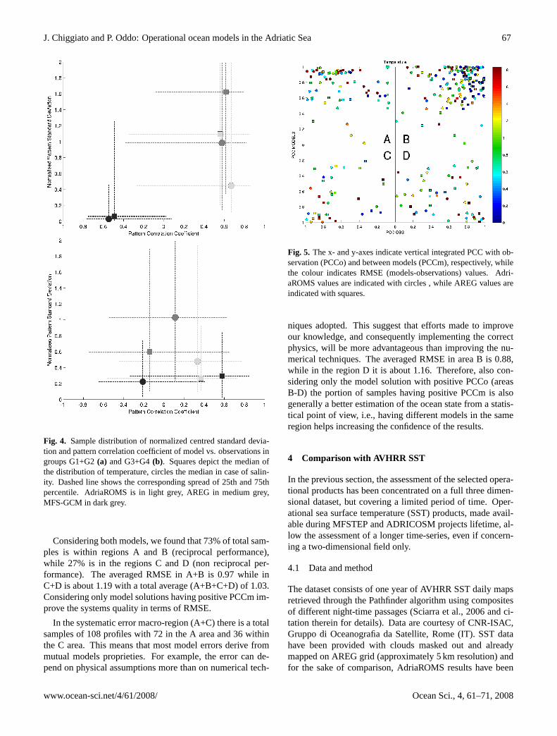
An additional analysis has been carried out to investigate themutual behaviour of the two regional operational systemsfrom a statistical point of view. For this aim, Pattern Corre-lation Coefficient between models (PCCm), between modeland observations (PCCo) and RMSE have been combined, inthis case grouping all the CTD casts. Results of the compu-tation are shown in Fig. 5. On the basis of PCC values fourareas (A, B, C and D) have been defined: area A (high PCCmand low PCCo values) identifies mutual systematic model er-rors; area B (high values of both PCCm and PCCo) indicatesmutual skill; in area C (low values of both PCCm and PCCo)there are model-specific systematic errors and, finally, area D(low PCCm and high PCCo values) states for model-specificskill.



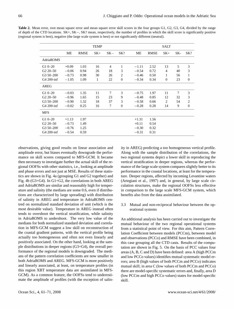
Fig. 4. Sample distribution of normalized centred standard devia-tion and pattern correlation coefficient of model vs. observations ingroups G1+G2(a) and G3+G4(b). Squares depict the median ofthe distribution of temperature, circles the median in case of salin-ity. Dashed line shows the corresponding spread of 25th and 75thpercentile. AdriaROMS is in light grey, AREG in medium grey,MFS-GCM in dark grey.

Considering both models, we found that 73% of total sam-ples is within regions A and B (reciprocal performance),while 27% is in the regions C and D (non reciprocal per-formance). The averaged RMSE in A+B is 0.97 while inC+D is about 1.19 with a total average (A+B+C+D) of 1.03.Considering only model solutions having positive PCCm im-prove the systems quality in terms of RMSE.

In the systematic error macro-region (A+C) there is a totalsamples of 108 profiles with 72 in the A area and 36 withinthe C area. This means that most model errors derive frommutual models proprieties. For example, the error can de-pend on physical assumptions more than on numerical tech-

Fig. 5. The x- and y-axes indicate vertical integrated PCC with ob-servation (PCCo) and between models (PCCm), respectively, whilethe colour indicates RMSE (models-observations) values. Adri-aROMS values are indicated with circles , while AREG values areindicated with squares.

niques adopted. This suggest that efforts made to improveour knowledge, and consequently implementing the correctphysics, will be more advantageous than improving the nu-merical techniques. The averaged RMSE in area B is 0.88,while in the region D it is about 1.16. Therefore, also con-sidering only the model solution with positive PCCo (areasB-D) the portion of samples having positive PCCm is alsogenerally a better estimation of the ocean state from a statis-tical point of view, i.e., having different models in the sameregion helps increasing the confidence of the results.

4 Comparison with AVHRR SST

In the previous section, the assessment of the selected opera-tional products has been concentrated on a full three dimen-sional dataset, but covering a limited period of time. Oper-ational sea surface temperature (SST) products, made avail-able during MFSTEP and ADRICOSM projects lifetime, al-low the assessment of a longer time-series, even if concern-ing a two-dimensional field only.

4.1 Data and method

The dataset consists of one year of AVHRR SST daily mapsretrieved through the Pathfinder algorithm using compositesof different night-time passages (Sciarra et al., 2006 and ci-tation therein for details). Data are courtesy of CNR-ISAC,Gruppo di Oceanografia da Satellite, Rome (IT). SST datahave been provided with clouds masked out and alreadymapped on AREG grid (approximately 5 km resolution) andfor the sake of comparison, AdriaROMS results have been



Fig. 6. Time series of monthly averaged root mean square error ofmodel vs. AVHRR-SST.

Fig. 7. Time series of monthly root mean squared error of modelvs. AVHRR-SST decomposed in mean error term (MB), standarddeviation error (STE), cross covariance error term (CCE) and cor-relation coefficient (R).

bilinearly interpolated onto the same grid. For equality in do-mains, this analysis is south-bounded at the latitude 40.7◦ N.MFS-GCM data are not considered in this analysis since theSSTs are used in the flux-correction procedure and thereforethey are not an independent dataset.

The comparison between model SST and AVHRR skinSST may become critical when the warm layer develops andeven worse in deeper regions (since model surface tempera-ture is indeed representative of a thick layer, because of theterrain-following vertical coordinate). The fact that SST im-ages are night-time images helps to minimize such biases.

Based on this dataset, the RMSE was computed monthlyon a basin-wide, aggregated subset of model errors. Com-pared to other possible approaches, as for example first es-timating over space the daily MSE and then averaging overtime, this formulation permits overcoming the cloud-cover

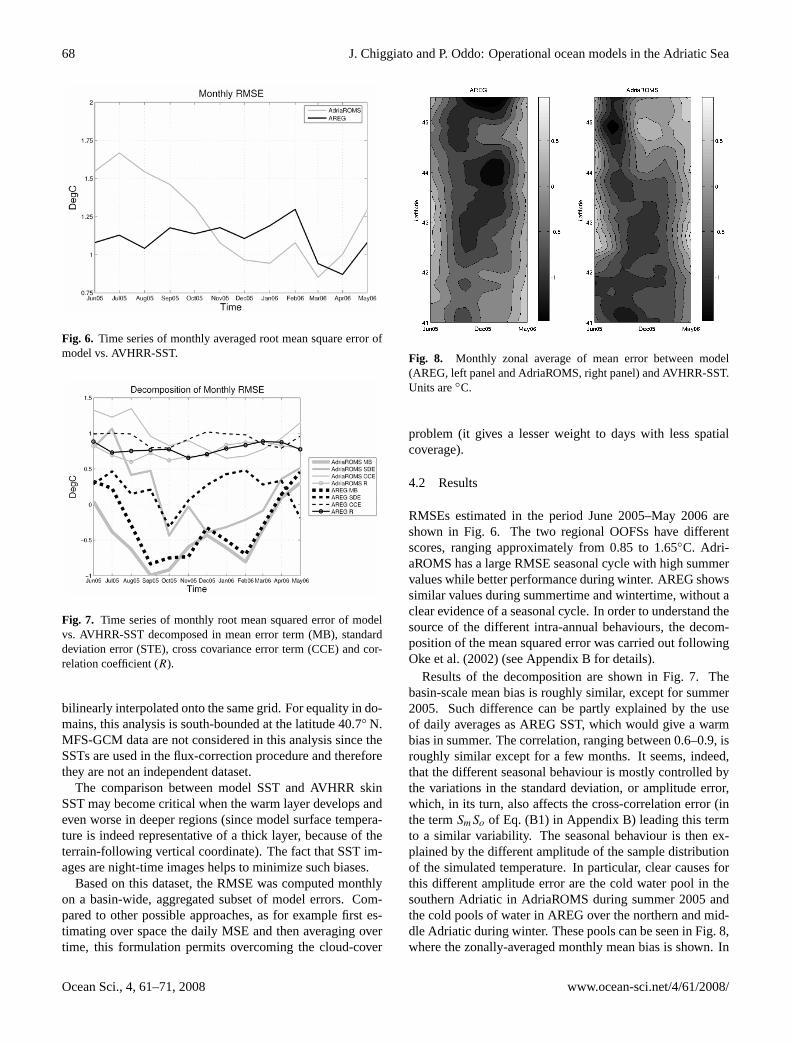
Fig. 8. Monthly zonal average of mean error between model(AREG, left panel and AdriaROMS, right panel) and AVHRR-SST.Units are◦C.

problem (it gives a lesser weight to days with less spatialcoverage).

4.2 Results

RMSEs estimated in the period June 2005–May 2006 areshown in Fig. 6. The two regional OOFSs have differentscores, ranging approximately from 0.85 to 1.65◦C. Adri-aROMS has a large RMSE seasonal cycle with high summervalues while better performance during winter. AREG showssimilar values during summertime and wintertime, without aclear evidence of a seasonal cycle. In order to understand thesource of the different intra-annual behaviours, the decom-position of the mean squared error was carried out followingOke et al. (2002) (see Appendix B for details).

Results of the decomposition are shown in Fig. 7. Thebasin-scale mean bias is roughly similar, except for summer2005. Such difference can be partly explained by the useof daily averages as AREG SST, which would give a warmbias in summer. The correlation, ranging between 0.6–0.9, isroughly similar except for a few months. It seems, indeed,that the different seasonal behaviour is mostly controlled bythe variations in the standard deviation, or amplitude error,which, in its turn, also affects the cross-correlation error (inthe termSmSo of Eq. (B1) in Appendix B) leading this termto a similar variability. The seasonal behaviour is then ex-plained by the different amplitude of the sample distributionof the simulated temperature. In particular, clear causes forthis different amplitude error are the cold water pool in thesouthern Adriatic in AdriaROMS during summer 2005 andthe cold pools of water in AREG over the northern and mid-dle Adriatic during winter. These pools can be seen in Fig. 8,where the zonally-averaged monthly mean bias is shown. In



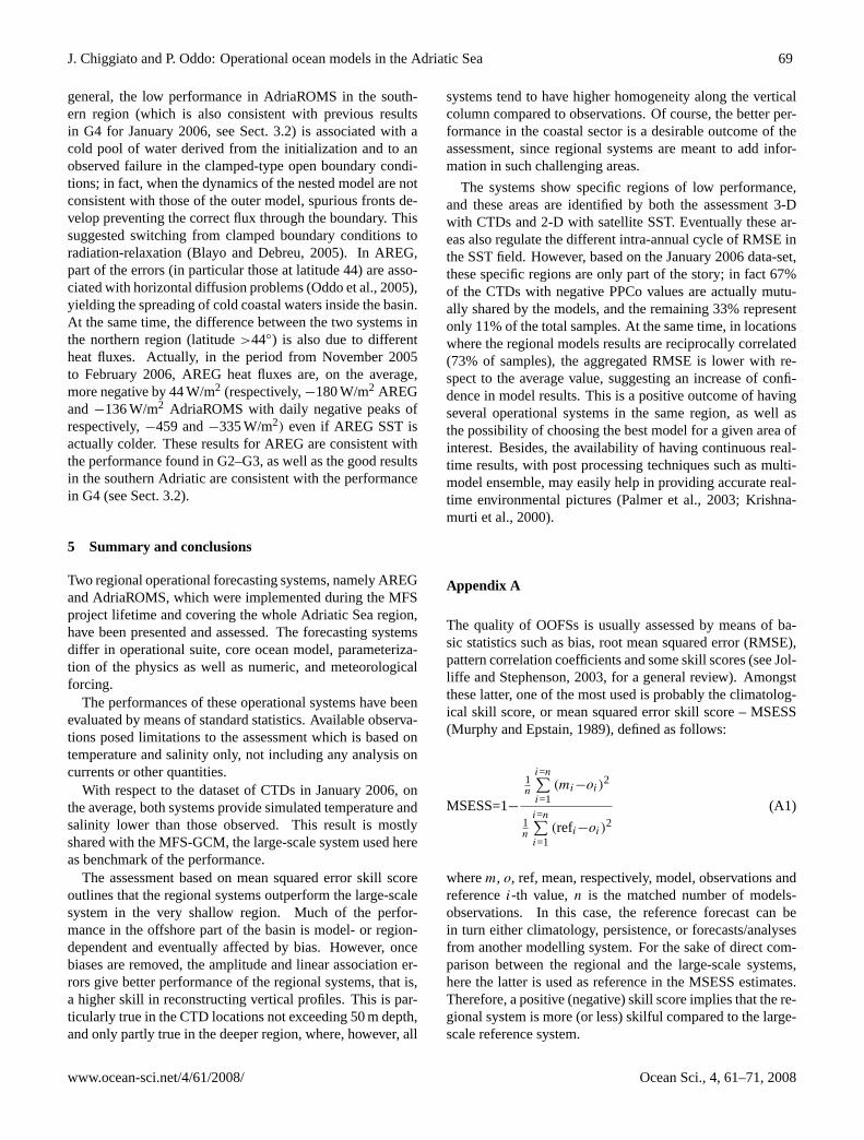
general, the low performance in AdriaROMS in the south-ern region (which is also consistent with previous resultsin G4 for January 2006, see Sect. 3.2) is associated with acold pool of water derived from the initialization and to anobserved failure in the clamped-type open boundary condi-tions; in fact, when the dynamics of the nested model are notconsistent with those of the outer model, spurious fronts de-velop preventing the correct flux through the boundary. Thissuggested switching from clamped boundary conditions toradiation-relaxation (Blayo and Debreu, 2005). In AREG,part of the errors (in particular those at latitude 44) are asso-ciated with horizontal diffusion problems (Oddo et al., 2005),yielding the spreading of cold coastal waters inside the basin.At the same time, the difference between the two systems inthe northern region (latitude>44◦) is also due to differentheat fluxes. Actually, in the period from November 2005to February 2006, AREG heat fluxes are, on the average,more negative by 44 W/m2 (respectively,−180 W/m2 AREGand−136 W/m2 AdriaROMS with daily negative peaks ofrespectively,−459 and−335 W/m2) even if AREG SST isactually colder. These results for AREG are consistent withthe performance found in G2–G3, as well as the good resultsin the southern Adriatic are consistent with the performancein G4 (see Sect. 3.2).

5 Summary and conclusions

Two regional operational forecasting systems, namely AREGand AdriaROMS, which were implemented during the MFSproject lifetime and covering the whole Adriatic Sea region,have been presented and assessed. The forecasting systemsdiffer in operational suite, core ocean model, parameteriza-tion of the physics as well as numeric, and meteorologicalforcing.

The performances of these operational systems have beenevaluated by means of standard statistics. Available observa-tions posed limitations to the assessment which is based ontemperature and salinity only, not including any analysis oncurrents or other quantities.

With respect to the dataset of CTDs in January 2006, onthe average, both systems provide simulated temperature andsalinity lower than those observed. This result is mostlyshared with the MFS-GCM, the large-scale system used hereas benchmark of the performance.

The assessment based on mean squared error skill scoreoutlines that the regional systems outperform the large-scalesystem in the very shallow region. Much of the perfor-mance in the offshore part of the basin is model- or region-dependent and eventually affected by bias. However, oncebiases are removed, the amplitude and linear association er-rors give better performance of the regional systems, that is,a higher skill in reconstructing vertical profiles. This is par-ticularly true in the CTD locations not exceeding 50 m depth,and only partly true in the deeper region, where, however, all

systems tend to have higher homogeneity along the verticalcolumn compared to observations. Of course, the better per-formance in the coastal sector is a desirable outcome of theassessment, since regional systems are meant to add infor-mation in such challenging areas.

The systems show specific regions of low performance,and these areas are identified by both the assessment 3-Dwith CTDs and 2-D with satellite SST. Eventually these ar-eas also regulate the different intra-annual cycle of RMSE inthe SST field. However, based on the January 2006 data-set,these specific regions are only part of the story; in fact 67%of the CTDs with negative PPCo values are actually mutu-ally shared by the models, and the remaining 33% representonly 11% of the total samples. At the same time, in locationswhere the regional models results are reciprocally correlated(73% of samples), the aggregated RMSE is lower with re-spect to the average value, suggesting an increase of confi-dence in model results. This is a positive outcome of havingseveral operational systems in the same region, as well asthe possibility of choosing the best model for a given area ofinterest. Besides, the availability of having continuous real-time results, with post processing techniques such as multi-model ensemble, may easily help in providing accurate real-time environmental pictures (Palmer et al., 2003; Krishna-murti et al., 2000).

Appendix A

The quality of OOFSs is usually assessed by means of ba-sic statistics such as bias, root mean squared error (RMSE),pattern correlation coefficients and some skill scores (see Jol-liffe and Stephenson, 2003, for a general review). Amongstthese latter, one of the most used is probably the climatolog-ical skill score, or mean squared error skill score – MSESS(Murphy and Epstain, 1989), defined as follows:

MSESS=1−

1n

i=n∑i=1

(mi−oi)2

1n

i=n∑i=1

(refi−oi)2

(A1)

wherem, o, ref, mean, respectively, model, observations andreferencei-th value,n is the matched number of models-observations. In this case, the reference forecast can bein turn either climatology, persistence, or forecasts/analysesfrom another modelling system. For the sake of direct com-parison between the regional and the large-scale systems,here the latter is used as reference in the MSESS estimates.Therefore, a positive (negative) skill score implies that the re-gional system is more (or less) skilful compared to the large-scale reference system.



Appendix B

Mean squared errors can be decomposed in many ways; fol-lowing the Oke et al. (2002) approach and nomenclature,MSE can be split into:

MSE=MB2+ SDE2

+ 2SmSo (1−CC) ; (B1)

where MB=m−o is the mean bias, SDE=Sm−So is the stan-dard deviation error,(2SmSo (1 − CC))

12 the cross correla-

tion error, withm and o representing, respectively, modeland observed values,S the standard deviation of the sampledistribution, CC the correlation coefficient.

Acknowledgement.The authors greatly acknowledge ISAC-CNRGruppo di Oceanografia da Satellite for AVHRR and CTD data.This work has been carried out within the framework of the“Mediterranean Forecasting System: Toward Environmental Pre-dictions” project, EC Contract EVK3-CT2002-00075, as well asADRICOSM project funded by the Italian Ministry of Environmentand Territory (through the University of Bologna, Centro Interdi-partimentale per le Ricerche di Scienze Ambientali, Ravenna, Italy)and European INTERREG III CADSES – CADSELAND project.J. C. acknowledges H. Arango, J. Wilkin (Rutgers University)and R. P. Signell, J. Warner (USGS) for their useful suggestionsduring the implementation phase of AdriaROMS, as well as theresearch contract 2007 ARPA-SIM – CNR-ISMAR and ONR grantN00014-05-1-0730.

Edited by: E. J. M. Delhez

References

Artegiani, A., Bregant, D., Paschini, E., Pinardi, N., Raicich, F., andRusso, A.: The Adriatic Sea General Circulation, Part I: Air-SeaInteraction and Water Mass Structure, J. Phys. Oceanogr., 27,1492–1514, 1997.

Blayo, E. and Debreu, L.: Revisiting open boundary conditionsfrom the point of view of characteristic variables, Ocean Model.,9, 231–252, 2005.

Blumberg, A. F. and Mellor, G. L.: A description of athree-dimensional coastal ocean circulation model, in: Three-dimensional coastal ocean models, edited by: Heaps, N. S.,American Geophysical Union, Washington D.C, 208 pp., 1987.

Budyko, K.: Climate and Life, Academic Press, 508 pp., 1974.Cushman-Roisin, B. and Naimie, C. E.: A 3D finite-element model

of the Adriatic tides, J. Mar. Syst., 37, 279–297, 2002.DeMey, P. and Benkiran, M.: A multivariate Reduced-order Op-

timal Interpolation Method and its application to the Mediter-ranean Basin-scale Circulation, in: Ocean Forecasting, edited by:Pinardi, N. and Woods, J., 281–305, 2002.

Demirov, E., Pinardi, N., Fratianni, C., Tonani, M., Giacomelli, L.,and DeMey, P.: Assimilation scheme of Mediterranean Forecast-ing System: Operational implementation, Ann. Geophys., 21,189–204, 2003,http://www.ann-geophys.net/21/189/2003/.

Dobricic, S., Pinardi, N., Adani, M., Tonani, M., Fratianni, C.,Bonazzi, A., and Fernandez, V.: Daily oceanographic analysesby Mediterranean Forecasting System at the basin scale, Ocean

Sci., 3, 149–157, 2007,http://www.ocean-sci.net/3/149/2007/.

Fairall, C. W., Bradley, E. F., Rogers, D. P., Edson, J. B., and Young,G. S.: Bulk parameterization of air-sea fluxes for Tropical OceanGlobal Atmosphere Coupled-Ocean Atmosphere Response Ex-periment, J. Geophys. Res., 101(C2), 3747–3764, 1996.

Flather, R. A.: A tidal model of the northwest European continen-tal shelf, Memories de la Societe Royale des Sciences de Liege,6(10), 141–164, 1976.

Joliffe, I. T. and Stephenson, D. B.: Forecast Verification, A Practi-tioner’s Guide in Atmospheric Science, John Wiley & Sons, 240pp., 2003.

Krishnamurti, T. N., Kishtawal, C. M., Zhang, Z., LaRow, T.,Bacjiochi, D., and Williford, E.: Multimodel Ensemble Forecastfor Weather and Seasonal Climate, J. Climate, 13, 4196–4216,2000.

Madec, G., Delecluse, P., Imbard, M., and Levy, C.: OPA 8.1 OceanGeneral Circulation Model reference manual. Note du Pole demodelisation, Institut Pierre-Simon Laplace, 11, 91 pp., 1998.

Mellor, G. L. and Yamada, T.: Development of a turbulence clo-sure model for geophysical fluid problems, Rev. Geophys. SpacePhys., 20, 851–875, 1982.

Murphy A. H. and Epstein, E. S.: Skill scores and correlation coef-ficients in model verification, Mon. Weather Rev., 119, 572–581,1989.

Oddo, P., Pinardi, N., and Zavatarelli, M.: A numerical study ofthe interannual variability of the Adriatic Sea (2000–2002), Sci.Total Environ., 353, 39–56, 2005.

Oddo, P., Pinardi, N., Zavatarelli, M., and Coluccelli, A.: The Adri-atic Basin Forecasting System, Acta Adriatica, 47 (Suppl.), 169–184, 2006.

Oke, P. R., Allen, J. S., Miller, R. N., Egbert, G. D., Austin, J. A.,Barth, J. A., Boyd, T. J., Kosro, P. M., and Levine, M. D.: A mod-elling study of the three-dimensional continental shelf circulationoff Oregon. Part I: Model-Data Comparison, J. Phys. Oceanogr.,32, 1360–1382, 2002.

Onken, R., Robinson, A. R., Kantha, L., Lozano, C. J., Haley, P. J.,and Carniel, S.: A rapid response nowcast/forecast system usingmultiply nested ocean models and distributed data systems, J.Mar. Syst., 56, 45–66, 2005.

Palmer, T. N., Alessandri, A., Andersen, U., Cantelaube, P., Davey,M., Delecluse, P., Deque, M., Dıez, E., Doblas-Reyes, F. J., Fed-dersen, H., Graham, R., Gualdi, S., Gueremy, J. F., Hagedorn,R., Hoshen, M., Keenlyside, N., Latif, M., Lazar, A., Maison-nave, E., Marletto, V., Morse, A. P., Orfila, B., Rogel, P., Terres,J. M., and Thomson, M. C.: Development of a European Multi-Model Ensemble System for Seasonal to Inter-Annual Prediction(DEMETER), B. Am. Meteor. Soc., 85, 853–872, 2003.

Pinardi, N., Allen, I., Demirov, E., De Mey, P., Korres, G., Las-caratos, A., Le Traon, P.-Y., Maillard, C., Manzella, G., andTziavos, C.: The Mediterranean ocean Forecasting System: firstphase of implementation (1998–2001), Ann. Geophys., 21, 3–20,2003,http://www.ann-geophys.net/21/3/2003/.

Raicich, F.: On the fresh water balance of the Adriatic Sea, J. Mar.Syst., 9, 305–319, 1996.

Robinson, A. R. and Sellschopp, J.: Rapid assessment of the coastalocean environment, in: Ocean Forecasting: Conceptual Basisand Applications, edited by: Pinardi, N. and Woods, J., Springer-


http://www.ann-geophys.net/21/189/2003/

http://www.ocean-sci.net/3/149/2007/



Verlag, NY, 199–229, 2002.Sannino, G. M., Bargagli, A., and Artale, V.: Numerical modelling

of the mean exchange through the Strait of Gibraltar, J. Geophys.Res., 107(C8), 3094, doi:10.1029/2001JC000929, 2002.

Sciarra, R., Bohm, E., D’Acunzo, E., and Santoleri, R.: The largescale observing system component of ADRICOSM: the satellitesystem, Acta Adriatica, 47 (Suppl.), 51–64, 2006.

Shchepetkin, A. and McWilliams J. C.: Quasi-monotone advec-tion schemes based on explicit locally adaptive dissipation, Mon.Weather Rev., 126, 1541–1580, 1998.

Shchepetkin, A. F. and McWilliams, J. C.: A method for ComputingHorizontal Pressure-Gradient Force in an Oceanic Model witha Non-Aligned Vertical Coordinate, J. Geophys. Res., 108(C3),3090. doi:10.1029/2001JC001047, 2003.

Shchepetkin, A. F. and McWilliams, J. C.: The Regional OceanModelling System: A Split-Explicit, Free-Surface, Topography-Following-Coordinate Oceanic Model, Ocean Model., 9, 347–404, 2005.

Signell, R. P., Carniel, S., Cavalieri, L., Chiggiato, J., Doyle, J.,Pullen, J., and Sclavo, M.: Assessment of wind quality foroceanographic modeling in semienclosed basins, J. Mar. Syst.,53, 217–233, 2005

Smolarkiewicz, P. K.: A fully multidimensional positive definite ad-vection transport algorithm with small implicit diffusion, J. Com-put. Phys., 54, 325–362, 1984.

Steppeler, J., Doms, G., Shatter, U., Bitzer, H. W., Gassmann, A.,Damrath, U., and Gregoric, G.: Meso-gamma scale forecasts us-ing the nonhydrostatic model LM, Meteorol. Atmos. Phys., 82,75–96, 2003.

Tonani, M., Pinardi, N., Dobricic, S., Pujol, I. and Fratianni, C.:A high-resolution free-surface model of the Mediterranean Sea,Ocean Sci., 4, 1–14, 2008,http://www.ocean-sci.net/4/1/2008/.

Zavatarelli, M. and Pinardi, N.: The Adriatic Sea Modelling Sys-tem: a nested Approach, Ann. Geophys., 21, 345–364, 2003,http://www.ann-geophys.net/21/345/2003/.


http://www.ocean-sci.net/4/1/2008/


Documents

Operational ocean models in the Adriatic Sea: a skill