Embed Size (px)
Citation preview
Operational modal analysis on a wind turbine blade
F. Marulo1, G. Petrone
1, V. D’Alessandro
1, E. Di Lorenzo
1,2
1University of Naples “Federico II”, Department of Industrial Engineering,
Via Claudio 21, 80125, Naples, Italy
e-mail: [email protected]
2LMS, A Siemens Business, RTD Test Division,
Interleuvenlaan 68, 3001, Leuven, Belgium
Abstract The structural integrity of blades is critical in order to allow the operation of a wind turbine. An
appropriate knowledge about their dynamic characteristics is desired in early design stages too. The effect
of some local failure on the modal parameters of a wind turbine blade is experimentally investigated. The
investigated wind turbine blade is 6.4 m long and is made of glass fibers combined with epoxy resin.
During the tests, the blade is assumed to be clamped at the root. In order to identify the effect of some
failures on the modal parameters, the experimental campaign is divided in several steps: (i) an operational
modal analysis to extract the modal parameters before the failure; (ii) a static test, in which the blade
exhibits one or more failures; (iii) another operational modal analysis on the damaged structure.
Experimental results reveal a decrease in the natural frequencies and an increase of the estimated modal
damping of the structure. The reduction in natural frequencies is a result of a decrease of the stiffness of
the structure because of some structural failures.
1 Introduction
Performing modal tests on large structures such as wind turbines, buildings, bridges and airplanes is a
challenging task. The problem is not in measuring the responses, but in exciting the structures. Wind
turbines are huge and flexible structures with aerodynamic and gravitational forces acting on the rotating
blades. Excessive structural vibrations have always been a design concern. Output-only modal analysis
has been developed, in its first attempt, for determining the modal parameters of a wind turbine. It was
called Natural Excitation Testing (NExT), rather than Operational Modal Analysis (OMA). A critical step
in the development of NExT was to find a function that could be measured from operational data and that
possessed a clear relationship with the modal parameters of the structure [1]. The selected function was
the so called cross-correlation between responses without a measurement of the input forces. The NExT
procedure was a predecessor to the commonly used OMA techniques. Although the first application of an
OMA methodology was related to a vertical-axis wind turbine, not many other applications to wind
turbines were studied later on. The main reason is the fact that most of the OMA assumptions are violated
by operating wind turbines.
The structural integrity of blades is critical in order to allow the operation of a wind turbine. Modal
parameters are directly influenced by the physical properties of the structure. So, any change in the
physical properties should cause a change in its modal parameters and it can be used for Structural Health
Monitoring (SHM) purposes. A SHM technique should be implemented for on-line continuous monitoring
of wind turbines by comparing the differences between the monitored modal parameters and their baseline
values. A warning level would indicate when the blades are going toward a physical damage.

2 Geometry and materials
2.1 Geometry
The investigated structure is a 6.5 meter all fiberglass blade from a 30 kW wind turbine. Two airfoils were
used for the blade sections: the first with a maximum thickness of 25% used from the root up to 27% of
the radius, and the second blade with a maximum thickness of 21% used by 30% up to the end. The two
airfoils were combined with a connection one.
(a) (b)
Figure 1: Geometries of the airfoils with 25% (a) and 21% (b) as maximum thickness.
Chord and twist distribution was obtained by means of an optimization code in which the maximum area
was fixed and the requirement was the nominal rotation speed of 80 rpm. The main geometrical
parameters are reported in Figure 2a while from Figure 2b it have to be note the reduced section of the
free edge in order to reduce the aerodynamic noise.
(a)
(b)
Figure 2: Views of the blade.
2.2 Materials
The wind turbine blade is made of a high performance foam core (DIAB Divinycell H45), offering
excellent mechanical properties to low weight, arising from the combination of polyuren and pvc, covered
by fibreglass composites. The material properties of the core are listed in Table 1.
Two different configurations of glassfibres laminates were used: unidirectional and fabric. The material
properties of both the configurations, carried out by static test according to the ASTM standards and

indicated with the subscript 1 the longitudinal direction and the subscript 2 the transversal one, are listed
in Table 2.
Young’s
modulus
E [GPa]
Shear
modulus
G [GPa]
Poisson’s
ratio
ν
Mass
density
ρ [kg/m3]
Foam H 45 59.0 15.9 0.32 48
Table 1: Core mechanical properties.
Different configurations of the composite material (stacking sequence, number of plies) are distributed
along the blade span. In Figure 3 the different material configurations are shown by using different
colours.
Longitudinal
Young’s
modulus
E1 [GPa]
Transversal
Young’s
modulus
E2 [GPa]
Shear
modulus
G12 [GPa]
Poisson’s
ratio
ν
Mass
density
ρ [kg/m3]
unidirectional 30.0 7.0 4.0 0.22 2200
Fabric 15.6 15.6 4.0 0.27 2200
Table 2: Laminates mechanical properties.
Figure 3: Material distribution along the blade.
3 Experimental investigation
3.1 Operational Modal Analysis (OMA)
Operational Modal Analysis (OMA) technique allows extracting the modal parameters from vibration
response signal by means of auto and cross- correlations functions. The main difference compared to the
traditional experimental modal analysis is that it does not need the measurement of the input forces.
Structures under operating conditions or in situations where it is impossible to measure the input forces
can be tested. The information obtained by means of OMA can be used for several purposes such as the
improvement of numerical models, the prediction of the dynamic behavior of new designs, the
identification of the modal parameters of prototypes and the monitoring of systems in operating conditions
in order to predict in advance possible failures or damages.
It is possible to extend common identification methods to situations in which the input forces cannot be
measured. The system must comply with three main assumptions. It must be Linear Time Invariant, the
excitation forces must be represented by a flat white noise spectrum in the band of interest and they have
to be uncorrelated. The better these assumptions are fulfilled, the better the quality of the estimated modal
parameters.
3.1.1 Operational Polymax
Several OMA techniques have been developed and evaluated in the past years. In this paper, the Polymax
method [2] has been selected to perform the operational modal analysis. It has been developed as a
polyreference version of the least-squares complex frequency-domain (LSCF) estimation method using a
so-called right matrix-fraction model. In case of Experimental Modal Analysis (EMA), the modal
decomposition of an FRF matrix [H(ω)] is described in Equation (1):
*
*
1
)(i
H
iiM
i i
T
ii
j
lv
j
lvH
(1)
where l is the number of outputs; M is the number of modes, * is the complex conjugate operator, H is the
complex conjugate transpose of a matrix, {vi} are the mode shapes, are the modal participation factors and
λi are the poles.
The relationship that occurs between poles, eigenfrequencies ωi and damping ratios ξi is:
iiiiii j 2* 1 (2)
The input spectra [Suu(ω)] and output spectra [Syy(ω)] of a system represented by the FRF matrix are
related as:
Huuyy HSHS )()()()( (3)
Unlike in EMA, where FRFs between input and outputs are used, OMA uses output-only data. A leakage-
free and Hanning-window free pre-processing method is used to estimate the power and cross spectra. The
weighted correlogram approach was adopted: correlations with positive time lags are computed from the
time data; an exponential window is applied to reduce leakage and the influence of the noisier higher time
lag correlation samples; and finally the DFT of the windowed correlation samples is taken. An exponential
window is compatible with the modal model and therefore, the pole estimates can be corrected for the
application of such a window. More details about this pre-processing and the comparison with the more
classical Welch's averaged periodogram estimate (involving Hanning windows) can be found in [3].
The Polymax algorithm greatly facilitates the operational modal parameter estimation process by
producing extremely clear stabilization diagrams, making the pole selection a lot easier by means of
estimating unstable poles (i.e. mathematical or noise modes) with negative damping making them
relatively easy to separate from the stable poles (i.e. system modes) [2, 3].
3.1.2 Stochastic subspace identification
Another advanced OMA method is the Stochastic Subspace Identification (SSI) one. The term subspace
means that the method identifies a state-space model and that it involves a Singular Value Decomposition
(SVD) truncation step. There are several variants in this class of methods including Canonical Variate
Analysis (CVA) and Balanced Realization (BR).
In this method a so-called stochastic state space model is identified from output correlations or directly
from measured output data [7]. The state space model is written is written in Equation (5):
kkk
kkk
vCxy
wAxx
1 (4)
where yk is the sampled output vector, xk is the discrete state vector, wk is the process noise due to
disturbances and unknown excitation of the structure, vk is the measurement noise, mainly due to sensor
inaccuracy, but also to the unknown excitation of the structure; k is the time instant. The matrix A is the
state transition matrix that completely describes the dynamics of the system by its eigenvalues; C is the
output matrix. The only known terms in Equation (5) are the output measurements yk and the challenge is
to determine the system matrices A, C from which the modal parameters can be derived.
The derivation of the modal parameters starts with the eigenvalue decomposition of A:
1 dA (5)
where Ψ is the eigenvector matrix and Λd is a diagonal matrix containing the discrete-time eigenvalues μi
which are related to the continuous-time eigenvalues λi as:
)exp( tii (6)
The eigenfrequencies and damping ratios are related to λi as expressed in Equation (2). Finally, the mode
shapes are found as:
CV (7)
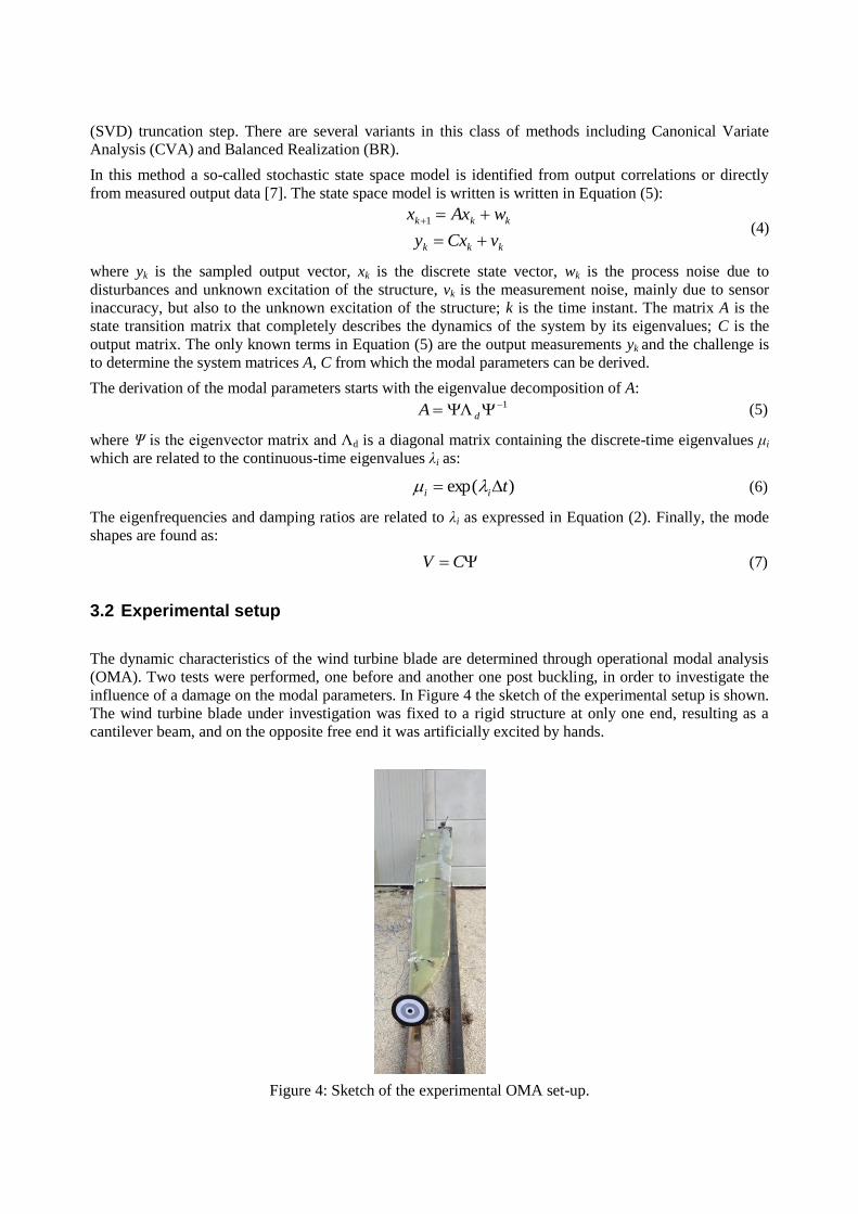
3.2 Experimental setup
The dynamic characteristics of the wind turbine blade are determined through operational modal analysis
(OMA). Two tests were performed, one before and another one post buckling, in order to investigate the
influence of a damage on the modal parameters. In Figure 4 the sketch of the experimental setup is shown.
The wind turbine blade under investigation was fixed to a rigid structure at only one end, resulting as a
cantilever beam, and on the opposite free end it was artificially excited by hands.
Figure 4: Sketch of the experimental OMA set-up.
The responses were recorded by using ten uni-axial accelerometers (PCB 352B10) located in two rows on
five sections along the blade in order to evaluate both flexural and torsional mode shapes. The
accelerometers were connected to the acquisition system LMS SCADAS III, which was connected to a
computer for the recording of the data. The whole acquisition process was controlled through the software
LMS Test.Lab, which is able to display, in real time, the Frequency Response Function of the excited
node on the experimental mesh. Vibration measurements were taken in the frequency range 0-256 Hz.
Once the experimental test was concluded, modal parameters were extracted through PolyMAX algorithm
and SSI method, both of them available again in LMS Test.Lab.
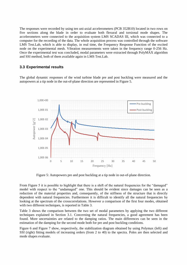
3.3 Experimental results
The global dynamic responses of the wind turbine blade pre and post buckling were measured and the
autopowers at a tip node in the out-of-plane direction are represented in Figure 5.
Figure 5: Autopowers pre and post buckling at a tip node in out-of-plane direction.
From Figure 5 it is possible to highlight that there is a shift of the natural frequencies for the “damaged”
model with respect to the “undamaged” one. This should be evident since damages can be seen as a
reduction of the material properties and, consequently, of the stiffness of the structure that is directly
dependent with natural frequencies. Furthermore it is difficult to identify all the natural frequencies by
looking at the spectrum of the crosscorrelations. However a comparison of the first four modes, obtained
with two different techniques, is reported in Table 3.
Table 3 shows the comparison between the two set of modal parameters by applying the two different
techniques explained in Section 3.1. Concerning the natural frequencies, a good agreement has been
found. More uncertainties are related to the damping ratios. The main differences can be seen in the
estimation of the damping for the second mode both for pre and post buckling conditions.
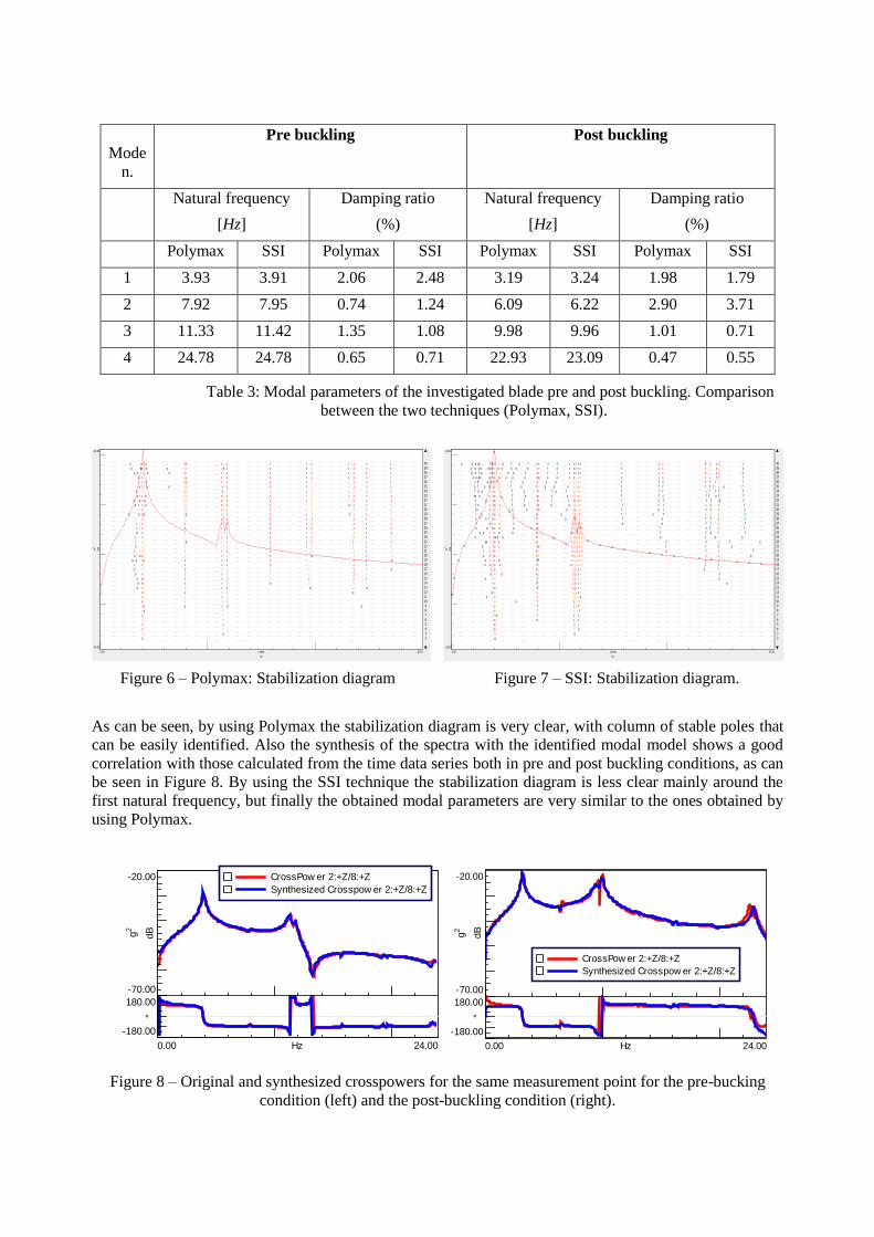
Figure 6 and Figure 7 show, respectively, the stabilization diagram obtained by using Polymax (left) and
SSI (right) fitting models of increasing orders (from 2 to 40) to the spectra. Poles are then selected and
mode shapes evaluate.
1,00E-06
1,00E-05
1,00E-04
1,00E-03
1,00E-02
1,00E-01
1,00E+00
0 5 10 15 20 25 30 35 40 45 50
Auto
po
wer
[g^2
]
Frequency [Hz]
Pre-buckling
Post-buckling
Mode
n.
Pre buckling Post buckling
Natural frequency
[Hz]
Damping ratio
(%)
Natural frequency
[Hz]
Damping ratio
(%)
Polymax SSI Polymax SSI Polymax SSI Polymax SSI
1 3.93 3.91 2.06 2.48 3.19 3.24 1.98 1.79
2 7.92 7.95 0.74 1.24 6.09 6.22 2.90 3.71
3 11.33 11.42 1.35 1.08 9.98 9.96 1.01 0.71
4 24.78 24.78 0.65 0.71 22.93 23.09 0.47 0.55
Table 3: Modal parameters of the investigated blade pre and post buckling. Comparison
between the two techniques (Polymax, SSI).
Figure 6 – Polymax: Stabilization diagram Figure 7 – SSI: Stabilization diagram.
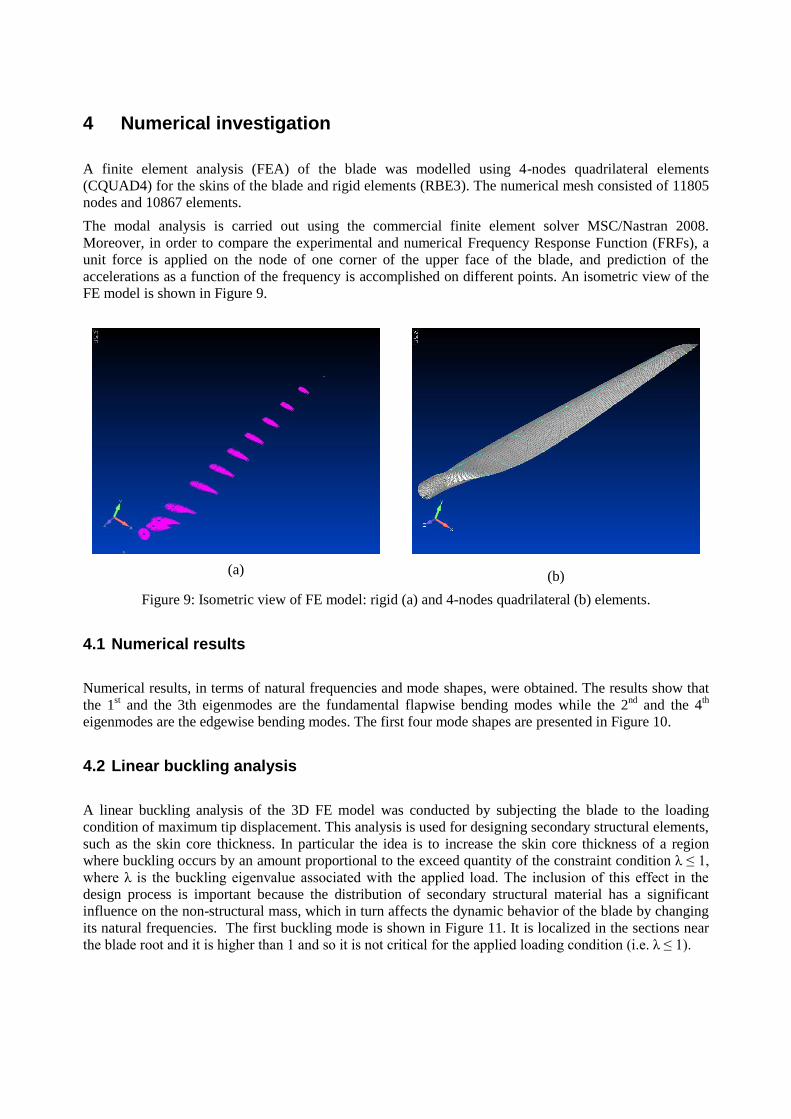
As can be seen, by using Polymax the stabilization diagram is very clear, with column of stable poles that
can be easily identified. Also the synthesis of the spectra with the identified modal model shows a good
correlation with those calculated from the time data series both in pre and post buckling conditions, as can
be seen in Figure 8. By using the SSI technique the stabilization diagram is less clear mainly around the
first natural frequency, but finally the obtained modal parameters are very similar to the ones obtained by
using Polymax.
24.000.00 Hz
-20.00
-70.00
dBg2
180.00
-180.00
°
CrossPow er 2:+Z/8:+Z
Synthesized Crosspow er 2:+Z/8:+Z
24.000.00 Hz
-20.00
-70.00
dBg2
180.00
-180.00
°
CrossPow er 2:+Z/8:+Z
Synthesized Crosspow er 2:+Z/8:+Z
Figure 8 – Original and synthesized crosspowers for the same measurement point for the pre-bucking
condition (left) and the post-buckling condition (right).
30.000.00 Linear
Hz
-18.92
-58.92
dB
g2
o
v o
s v
s s
v v
s v
vo v
vo o s o o
sv v v v
vv v s v
vvv s v v o
o vv v s s o v o
o ss s s v o v v v
o ss s s s v s s s
o vv s s v v v s v
o v s v v v v s v o
s s s s s s v s s
o o vo s s s s v s s o
o o sv v s v s v o v s v
s v vv v s s s v v v s v
o v v v v s s v v s v
s v vo v v s s s s s s
s s v s s s s s s s v
o s v v v s v v v s s
s s s s s s s s s s s
s s s s s s s s s s s
v s v vv s s s s s s s
o o svo vo vv s s s v o v s v
v s v v vs s s v v v s s
o s s o v v sv s s v v o s s v
o o s o v v sv s s s v v s s s
ov s o vv sv s s v v s s s s
o v v v s v vs v v s v v v s s
o s o o vv vs s s s v v s s s
s s o s s s s s s v v s s s
o s s s s s s s s s s s v
o o v o o s v s s s s s s s s s
o oov o o vv vo s s s v s s s s
o v vs o v s s s v s s s s s s s s
2
3
4
5
6
7
8
9
10
11
12
13
14
15
16
17
18
19
20
21
22
23
24
25
26
27
28
29
30
31
32
33
34
35
36
37
38
39
40
30.000.00 Linear
Hz
-18.92
-58.92
dB
g2
vo
vv o
ss v o
ss s v
ss o s s
vvo f s s
sv f v v f
sv f s v f
vv o f s v v
o vs s v v v o
o vv s v v s v
v ss ff s s s v
v sv sf s s s v o
o v vv vf s s v v o
o vv o ss s s s v d
s ss v ss s s s s o f
o o ss o dv o v v v v f f
o v sv o ff f s v v v v s s
o s ss v fvv s s v s v s s o
s s ss v dv s s s s s o f s f
o v ss s vso s s s s v f f d o
oo v ss o ss s s v v v d d s f o
o s sso o o fv v s v s v o f o v o
o o v sv o o ss s s s s v f f o f f
o o v osv d o ss v s v s s f d f s f
f vo v vv s d ss s s v s v o o f f s f
o o f ovv v f fv o v s v v f d f f d d
s o s sss s s ss o v s vs f o f s v s d
fo d vsv v o o fvo o s s vv f o f d d d d
f o s vss s f o vss o o vv vv f f f s d s f
f o v vss v f f vsv f s s s sv f d f f f df f
oo o s vss v f o ssv d o v v s v f f d f f o f f
f o o v vsv v f o vf v f o f vv vv f f f s f f f f
o f o s vss v f o fv o o o v v s v f f f f f f v o f
d ff o o fss v f o vs o o v v v vv f f d fv f f v f
o o oo o fss o o o o vso o o s s v vv d s s vv s f f f
o o f o s ovsv v o o f vsv f f s s s ss s s s fv v s s d
o o do o o f vv o o o o o vvv f d s s s sv s s s vv v s v d
o o o oo f of sv v o f o f svs d d s s s s s s s s fs s s s s
2
3
4
5
6
7
8
9
10
11
12
13
14
15
16
17
18
19
20
21
22
23
24
25
26
27
28
29
30
31
32
33
34
35
36
37
38
39
40
4 Numerical investigation
A finite element analysis (FEA) of the blade was modelled using 4-nodes quadrilateral elements
(CQUAD4) for the skins of the blade and rigid elements (RBE3). The numerical mesh consisted of 11805
nodes and 10867 elements.
The modal analysis is carried out using the commercial finite element solver MSC/Nastran 2008.
Moreover, in order to compare the experimental and numerical Frequency Response Function (FRFs), a
unit force is applied on the node of one corner of the upper face of the blade, and prediction of the
accelerations as a function of the frequency is accomplished on different points. An isometric view of the
FE model is shown in Figure 9.
(a) (b)
Figure 9: Isometric view of FE model: rigid (a) and 4-nodes quadrilateral (b) elements.
4.1 Numerical results
Numerical results, in terms of natural frequencies and mode shapes, were obtained. The results show that
the 1st and the 3th eigenmodes are the fundamental flapwise bending modes while the 2
nd and the 4
th
eigenmodes are the edgewise bending modes. The first four mode shapes are presented in Figure 10.
4.2 Linear buckling analysis
A linear buckling analysis of the 3D FE model was conducted by subjecting the blade to the loading
condition of maximum tip displacement. This analysis is used for designing secondary structural elements,
such as the skin core thickness. In particular the idea is to increase the skin core thickness of a region
where buckling occurs by an amount proportional to the exceed quantity of the constraint condition λ ≤ 1,
where λ is the buckling eigenvalue associated with the applied load. The inclusion of this effect in the
design process is important because the distribution of secondary structural material has a significant
influence on the non-structural mass, which in turn affects the dynamic behavior of the blade by changing
its natural frequencies. The first buckling mode is shown in Figure 11. It is localized in the sections near
the blade root and it is higher than 1 and so it is not critical for the applied loading condition (i.e. λ ≤ 1).

Mode 1
Flapwise bending
Mode 2
Edgewise bending
Mode 3
2nd
flapwise bending
Mode 4
2nd
edgewise bending
Figure 10: First four mode shapes of the wing turbine.
Figure 11: Close – up view of first buckling mode.
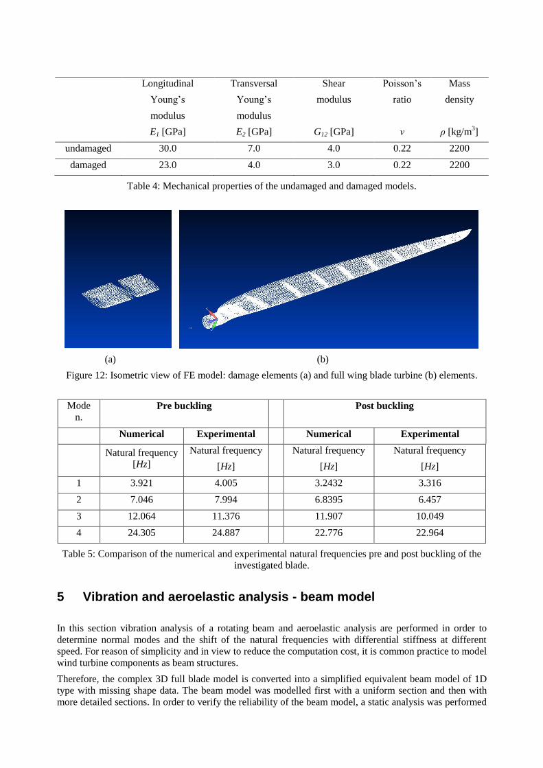
4.3 Turbine blade post buckling - numerical investigation and results
For the simulation of the damage it has been adopted the technique of reducing locally the material
properties of some elements of the whole structure. In particular to the elements belonging to the first two
sections the same material with lower mechanical properties has been attributed (Table 4).
Longitudinal
Young’s
modulus
E1 [GPa]
Transversal
Young’s
modulus
E2 [GPa]
Shear
modulus
G12 [GPa]
Poisson’s
ratio
ν
Mass
density
ρ [kg/m3]
undamaged 30.0 7.0 4.0 0.22 2200
damaged 23.0 4.0 3.0 0.22 2200
Table 4: Mechanical properties of the undamaged and damaged models.
(a) (b)
Figure 12: Isometric view of FE model: damage elements (a) and full wing blade turbine (b) elements.
Mode
n. Pre buckling Post buckling
Numerical Experimental Numerical Experimental
Natural frequency
[Hz]
Natural frequency
[Hz]
Natural frequency
[Hz]
Natural frequency
[Hz]
1 3.921 4.005 3.2432 3.316
2 7.046 7.994 6.8395 6.457
3 12.064 11.376 11.907 10.049
4 24.305 24.887 22.776 22.964
Table 5: Comparison of the numerical and experimental natural frequencies pre and post buckling of the
investigated blade.
5 Vibration and aeroelastic analysis - beam model
In this section vibration analysis of a rotating beam and aeroelastic analysis are performed in order to
determine normal modes and the shift of the natural frequencies with differential stiffness at different
speed. For reason of simplicity and in view to reduce the computation cost, it is common practice to model
wind turbine components as beam structures.
Therefore, the complex 3D full blade model is converted into a simplified equivalent beam model of 1D
type with missing shape data. The beam model was modelled first with a uniform section and then with
more detailed sections. In order to verify the reliability of the beam model, a static analysis was performed
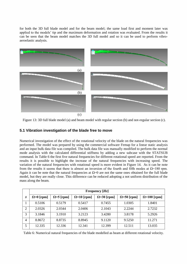
for both the 3D full blade model and for the beam model; the same load first and moment later was
applied to the models’ tip and the maximum deformation and rotation was evaluated. From the results it
can be seen that the beam model matches the 3D full model and so it can be used to perform vibro-
aeroelastic analysis.
(a)
(b)
(c)
Figure 13: 3D full blade model (a) and beam model with regular section (b) and not-regular section (c).
5.1 Vibration investigation of the blade free to move
Numerical investigation of the effect of the rotational velocity of the blade on the natural frequencies was
performed. The model was prepared by using the commercial software Femap for a linear static analysis
and an input bulk data file was compiled. The bulk data file was manually modified to perform the normal
mode analysis with the calculated differential stiffness by adding a new subcase with the STATSUB
command. In Table 6 the first five natural frequencies for different rotational speed are reported. From the
results it is possible to highlight the increase of the natural frequencies with increasing speed. The
variation of the natural frequencies with rotational speed is more evident in Figure 14. As it can be note
from the results it seems that there is almost an inversion of the fourth and fifth modes at Ω=180 rpm.
Again it can be note that the natural frequencies at Ω=0 are not the same ones obtained for the full blade
model, but they are really close. This difference can be reduced adopting a not uniform distribution of the
mass along the beam.
#
Frequency [Hz]
Ω=0 [rpm] Ω=5 [rpm] Ω=10 [rpm] Ω=30 [rpm] Ω=50 [rpm] Ω=100 [rpm]
1 0.5106 0.5179 0.5417 0.7455 1.0305 1.8401
2 2.0326 2.0344 2.0406 2.1043 2.2244 2.7232
3 3.1846 3.1910 3.2123 3.4280 3.8178 5.2926
4 8.8672 8.8735 8.8945 9.1120 9.5250 11.271
5 12.335 12.336 12.341 12.399 12.511 13.035
Table 6: Numerical natural frequencies of the blade modelled as beam at different rotational velocity.

Figure 14: Variation of natural frequencies at different rotational velocities.
5.2 Aeroelastic investigation
The increased flexibility of wind turbine blades justifies the need for considering aeroelastic effects for the
design of novel thinner blade sections. This paragraph presents an approach for aeroelastic calculation
based on classical method employed for aircraft surfaces including the centrifugal stiffness induced by the
rotational speed. In this preliminary aeroelastic calculations some simplification are considered. They
relate mainly to assume a rigid tower and a spanwise averaged wind speed. First hypothesis allows
avoiding the whirl flutter problem, which is outside the interest of this paper. The second hypothesis is
required by the selected method which, coming from airplane aeroelastic calculations, does not allow a
spanwise variable wind speed.
The equations of motion of a rotating beam, considering rotational stiffening effect, [4-8], are:
AAAGSSS KCMxKKxCxM (8)
where the matrices subscripted S (structural) and A (aerodynamic) are composed of elemental mass,
damping and stiffness terms and the stiffness matrix subscripted G stands for the centrifugal stiffening
contribution due to the rotational speed.
This equation allows the use of a standard aeroelastic solution as implemented inside commercial
software, like MSC/Nastran, provided the addition of the centrifugal stiffness [KG]. This matrix can be
computed separately and properly added to the structural stiffness matrix before the aeroelastic
computation. This operation is allowed to the user of the aeroelastic solution using the ALTER options
described in [8].
The procedure starts computing the [KS] + [KG (Ω)] matrices from a static case of the blade model loaded
by the centrifugal forces proportional to the rotational speed Ω. The stiffness matrices are then stored for
being recalled by the aeroelastic solution. These matrices replace the stiffness matrix computed by the
program before the computation of the aeroelastic effect. This approach is not automatic because it
requires two separate steps, but when implemented, it results in a not complex tool.
The validity of the approach has been firstly checked for structural dynamics computation, calculating the
variation of the frequencies (mode-shapes are generally not affected, for simple structures) due to
rotational speed Ω. The case presented here has specifically selected for highlighting the aeroelastic
0
2
4
6
8
10
12
14
16
18
20
0 50 100 150 200 250
Freq. [Hz]
Ω [rpm]
f1
f2
f3
f4
f5
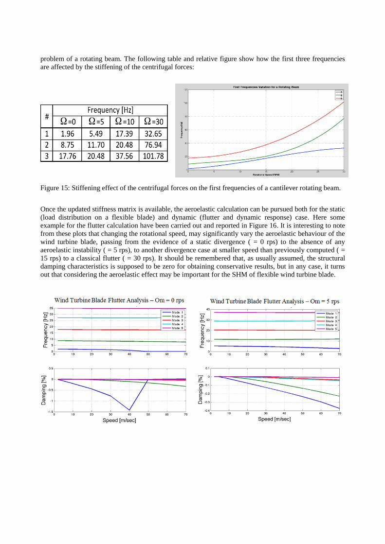
problem of a rotating beam. The following table and relative figure show how the first three frequencies
are affected by the stiffening of the centrifugal forces:
Figure 15: Stiffening effect of the centrifugal forces on the first frequencies of a cantilever rotating beam.
Once the updated stiffness matrix is available, the aeroelastic calculation can be pursued both for the static
(load distribution on a flexible blade) and dynamic (flutter and dynamic response) case. Here some
example for the flutter calculation have been carried out and reported in Figure 16. It is interesting to note
from these plots that changing the rotational speed, may significantly vary the aeroelastic behaviour of the
wind turbine blade, passing from the evidence of a static divergence ( = 0 rps) to the absence of any
aeroelastic instability ( = 5 rps), to another divergence case at smaller speed than previously computed ( =
15 rps) to a classical flutter ( = 30 rps). It should be remembered that, as usually assumed, the structural
damping characteristics is supposed to be zero for obtaining conservative results, but in any case, it turns
out that considering the aeroelastic effect may be important for the SHM of flexible wind turbine blade.
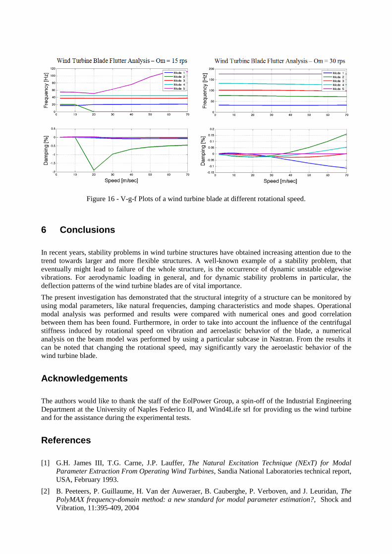
Figure 16 - V-g-f Plots of a wind turbine blade at different rotational speed.
6 Conclusions
In recent years, stability problems in wind turbine structures have obtained increasing attention due to the
trend towards larger and more flexible structures. A well-known example of a stability problem, that
eventually might lead to failure of the whole structure, is the occurrence of dynamic unstable edgewise
vibrations. For aerodynamic loading in general, and for dynamic stability problems in particular, the
deflection patterns of the wind turbine blades are of vital importance.
The present investigation has demonstrated that the structural integrity of a structure can be monitored by
using modal parameters, like natural frequencies, damping characteristics and mode shapes. Operational
modal analysis was performed and results were compared with numerical ones and good correlation
between them has been found. Furthermore, in order to take into account the influence of the centrifugal
stiffness induced by rotational speed on vibration and aeroelastic behavior of the blade, a numerical
analysis on the beam model was performed by using a particular subcase in Nastran. From the results it
can be noted that changing the rotational speed, may significantly vary the aeroelastic behavior of the
wind turbine blade.
Acknowledgements
The authors would like to thank the staff of the EolPower Group, a spin-off of the Industrial Engineering
Department at the University of Naples Federico II, and Wind4Life srl for providing us the wind turbine
and for the assistance during the experimental tests.
References
[1] G.H. James III, T.G. Carne, J.P. Lauffer, The Natural Excitation Technique (NExT) for Modal
Parameter Extraction From Operating Wind Turbines, Sandia National Laboratories technical report,
USA, February 1993.
[2] B. Peeteers, P. Guillaume, H. Van der Auweraer, B. Cauberghe, P. Verboven, and J. Leuridan, The
PolyMAX frequency-domain method: a new standard for modal parameter estimation?, Shock and
Vibration, 11:395-409, 2004

[3] B. Peeters, H. Van der Auweraer, F. Vanhollebeke, P. Guillaume, Operational modal analysis for
estimating the dynamic properties of a stadium structure during a football game, Shock and
Vibration, 14(4):283-303, 2007.
[4] E. Kosko, The Free Uncoupled Vibrations of a Uniformly Rotating Beam, Institute of Aerophisics,
University of Toronto, March 1960
[5] R.L. Bielawa, Rotary Wing Structural Dynamics and Aeroelasticity, AIAA Educational Series, 1992
[6] D.A. Spera, ed., Collected Papers on Wind Turbine Technology, NASA CR-195432, May 1995
[7] W.P. Rodden, MSC/Nastran Handbook for Aeroelastic Analysis, The MacNeal schwendler Corp.,
Report MSR-57, 1987
[8] M. Reymond, ed., DMAP Programmer’s Guide, MSC Software Doc 10013, 2013