Operation of a layer-oriented multiconjugate adaptive

Operation of a layer-orientedmulticonjugate adaptive optics systemin the partial illumination regime

Kalyan Kumar Radhakrishnan SanthakumariCarmelo ArcidiaconoThomas BertramFlorian BriegelThomas M. HerbstRoberto Ragazzoni

Kalyan Kumar Radhakrishnan Santhakumari, Carmelo Arcidiacono, Thomas Bertram, Florian Briegel,Thomas M. Herbst, Roberto Ragazzoni, “Operation of a layer-oriented multiconjugate adaptive opticssystem in the partial illumination regime,” J. Astron. Telesc. Instrum. Syst. 5(4), 049002 (2019),doi: 10.1117/1.JATIS.5.4.049002.

Downloaded From: https://www.spiedigitallibrary.org/journals/Journal-of-Astronomical-Telescopes,-Instruments,-and-Systems on 03 Feb 2022Terms of Use: https://www.spiedigitallibrary.org/terms-of-use

Operation of a layer-oriented multiconjugate adaptiveoptics system in the partial illumination regime

Kalyan Kumar Radhakrishnan Santhakumari,a,b,c,* Carmelo Arcidiacono,a Thomas Bertram,b Florian Briegel,bThomas M. Herbst,b and Roberto RagazzoniaaINAF-Osservatorio Astronomico di Padova, Vicolo dell’Osservatorio, Padova, ItalybMax Planck Institute for Astronomy, Heidelberg, GermanycInternational Max Planck Research School for Astronomy and Cosmic Physics at the University of Heidelberg, Heidelberg, Germany

Abstract. Multiconjugate adaptive optics (MCAO) promises uniform wide-field atmospheric correction.However, partial illumination of the layers at which the deformable mirrors are conjugated results in incompleteinformation about the full turbulence field. We report on a working solution to this difficulty for layer-orientedMCAO, including laboratory and on-sky demonstration with the LINC-NIRVANA instrument at the LargeBinocular Telescope. This approach has proven to be simple and stable. © The Authors. Published by SPIE under aCreative Commons Attribution 4.0 Unported License. Distribution or reproduction of this work in whole or in part requires full attribution of the originalpublication, including its DOI. [DOI: 10.1117/1.JATIS.5.4.049002]

Keywords: adaptive optics; multiconjugate adaptive optics; LINC-NIRVANA; layer-oriented; partial illumination; wavefrontreconstruction.

Paper 19015 received Feb. 4, 2019; accepted for publication Sep. 16, 2019; published online Oct. 14, 2019.

1 IntroductionIn the late 1980s, Beckers introduced the idea of multiconjugateadaptive optics (MCAO), a technique that could potentiallyincrease the isoplanatic patch substantially.1,2 The basicprinciple of MCAO is to use multiple stars measuring theatmospheric volume and correcting the turbulence using Ndeformable mirrors (DMs) conjugated to N layers. Althoughits feasibility had been earlier tested on-sky,3,4 the actualimplementation of MCAO for nighttime astronomy had to waituntil 2007, when the multiconjugate adaptive optics demon-strator (MAD) exhibited various MCAO schemes on the verylarge telescope.5,6 Despite a proposed upgrade7 and plans forfuture implementations,8–11 the only currently working night-time MCAO systems in the world are GeMS at the GeminiSouth telescope12,13 and LINC-NIRVANA (LN) at the LargeBinocular Telescope (LBT).14–17

MCAO systems promise to provide a uniform point spreadfunction (PSF) across a wide field-of-view (FoV), using multi-ple guide stars, either laser-guide stars (LGSs) or natural-guidestars (NGSs). “Star-oriented”1,18 and “layer-oriented”19 are twoapproaches for implementing MCAO. Star-oriented MCAO usesinformation from individual wavefront sensors (WFSs), one perstar, to computationally estimate the wavefront corresponding tothe conjugated layer via tomographic reconstruction of the fullturbulence volume. The signals are then sent to the respectiveDMs to correct the aberrations. In contrast to star-orientedMCAO, layer-oriented MCAO uses one WFS per controlledDM. In other words, light from multiple stars are used by aWFS, which senses the wavefront for a particular conjugationaltitude and then drives the corresponding DM.

For both the star- and layer-oriented approaches, NGSs can-not, in general, provide full information of the aberrations in thehigh-altitude layer since the diverging light paths give incom-plete coverage. This can, strictly speaking, also be true for

a LGS-based system. However, the arrangement of the LGSsis usually tuned to minimize such effects, and for this reason,we are not going to discuss this case any further. The partialillumination issue can be particularly severe when the wavefrontsensing turbulence layer is significantly different from that ofthe compensated scientific one, especially when combined witha correcting layer at a particularly higher altitude.

In the MAD implementation, the star-oriented approachneeded a separate interaction matrix calibration for eachasterism. The layer-oriented approach required only one suchcalibration.20 Although layer-oriented MCAO has the advan-tage of computational simplicity compared with star-orientedMCAO, solving the partial illumination issue is a prerequisitefor taking advantage of this. Note that for the star-oriented sce-nario, the partial illumination is addressed by the tomographicreconstruction.

In this paper, we describe a solution to the layer-orientedMCAO partial illumination issue in the context of the LN instru-ment. Section 2 describes the LN MCAO system and why solv-ing the partial illumination issue is essential. Section 3 explainsour solution. Results from laboratory and on-sky tests, alongwith discussion, appear in Sec. 4. Section 5 concludes withsummary and future prospects.

2 Partial Illumination Issue in the Context ofthe LINC-NIRVANA MCAO System

LN is a high-resolution near-infrared imager mounted at therear, bent-Gregorian foci of the LBT.17 LN is equipped withan advanced and unique layer-oriented MCAO module.21

Wavefront sensing is performed using multiple pyramids, whichacquire multiple NGSs from two different FoVs.22–24 In addi-tion, the design follows the layer-oriented scheme, which fore-sees the optical co-addition of the star footprints at the WFS,minimizing the read noise penalty and allowing fainter starsto be used for the sensing (as long as the total flux correspondsto the limiting magnitude for correction). We define footprint asthe projection of the telescope pupil through which the starlightpasses at a given altitude. This approach is expected to increase

*Address all correspondence to Kalyan Kumar Radhakrishnan Santhakumari,E-mail: [email protected]

Journal of Astronomical Telescopes, Instruments, and Systems 049002-1 Oct–Dec 2019 • Vol. 5(4)

Journal of Astronomical Telescopes, Instruments, and Systems 5(4), 049002 (Oct–Dec 2019)


https://doi.org/10.1117/1.JATIS.5.4.049002






mailto:[email protected]



the sky coverage in the typical case of being read noise limited.25

LN can provide uniform 2′ FoV correction for both “eyes” of theLBT, allowing us a larger field from which to choose fringe-tracking reference stars for eventual goal performing Fizeauinterferometric imaging.

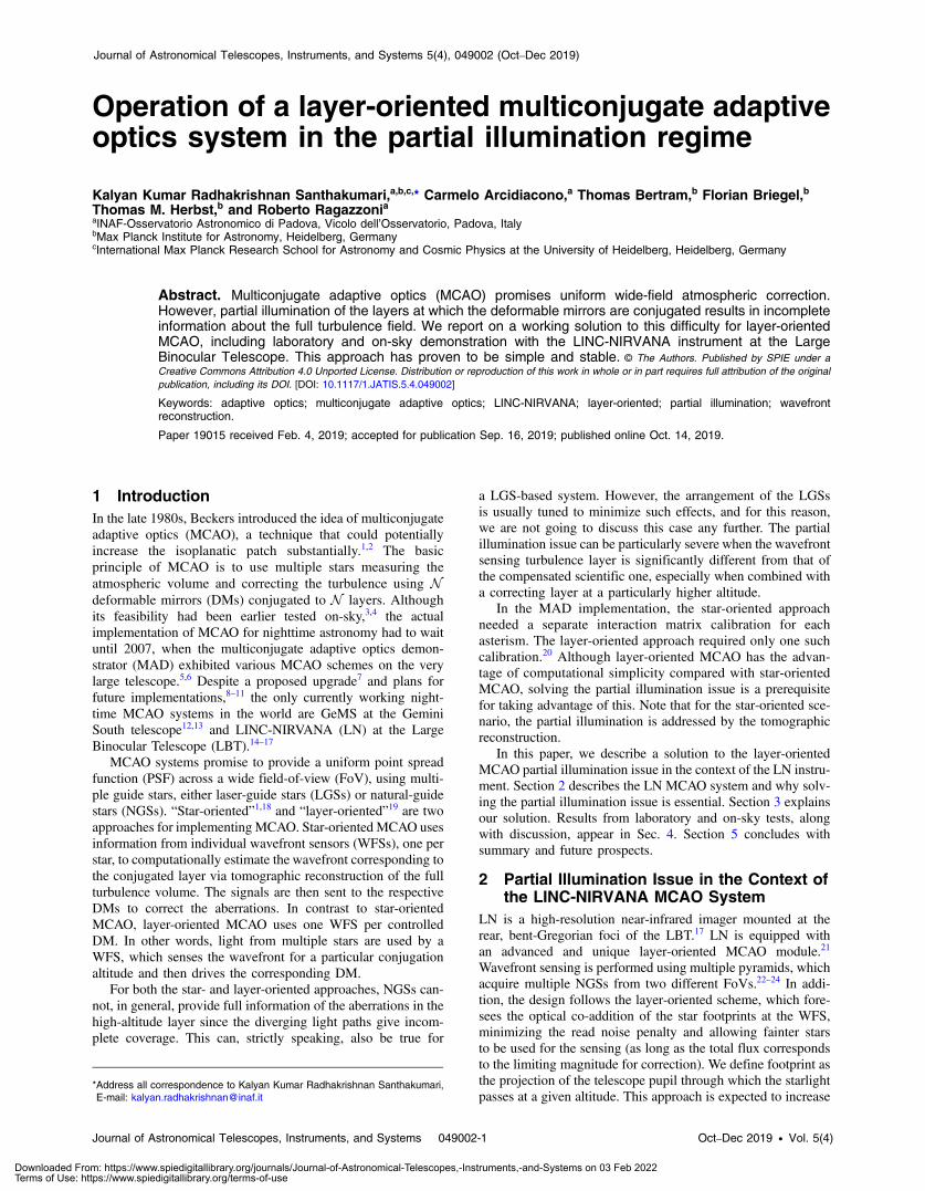
On each telescope, the atmospheric aberrations are sensed bytwo WFSs, one conjugated to the ground and the other to ahigher altitude, in order to sample the three-dimensional turbu-lence above the observatory.26,27 The ground-layer wavefrontsensors (GWSs) are conjugated to ∼100 m above the telescopeand drive the adaptive secondary mirrors (ASMs, 672 actuatorseach), using up to 12 natural stars from an annular 2’ to 6’ diam-eter FoV centered on the science field. The high-layer wavefrontsensors (HWSs) are conjugated to a high altitude, ∼7100 m

above the telescope pupil along the optical axis, and drive thetwo commercial Xinetics DMs (349 actuators each, hereafterhigh-altitude DMs)28 mounted on the LN bench. The HWSs canuse up to eight stars in the inner 2’ diameter FoV to measure theturbulence. LN MCAO correction is purely sequential and thetwo loops are independent in terms of control. This means thatthe HWSs receive the ground-layer corrected wavefront, makingthe loop control simpler, since we may use two separate recon-struction matrices. LN MCAO multiple-FoV approach, wherethe wavefront sensing is performed using stars lying in contigu-ous but not overlapping regions, is depicted in Fig. 1.

The reference star light focused at the tip of a four-sidedpyramid is split into four beams, forming, through a commonoptics, four pupil images on the WFS CCD. The pixels may bebinned on-chip, depending on the flux of the stars. Binning thisway reduces the equivalent readout noise on the individual sub-apertures. This improvement, coupled with the well-known sen-sitivity gain,29,30 is a direct benefit of pyramid wavefrontsensing. Comparing the local fluxes in the same subapertureof the four pupil images gives the local tilt.22 Note that for theground layer, the nominal star footprints overlap perfectly.Optical co-addition increases the signal-to-noise ratio (SNR) for

each subaperture uniformly for the ground layer (the purpleshaded region in Fig. 1).

At higher layers, the footprints of the stars are spatiallydecorrelated, and their positions depend on the star coordinates.In our case, by design, the high-altitude DM covers the foot-prints from any source within the 2’ FoV. This area is calledthe metapupil. It is the projection of the FoV at the conjugatedaltitude depicted by the yellow shaded region within the redcircle in Fig. 1. For LN, the diameter of the metapupil is about1.5 times that of a single pupil.

Depending on the asterism, only a part of the metapupil maybe illuminated (for example, see Figs. 2 and 3). In this instance,the slopes in the illuminated region can be directly measured,whereas there is no information about the atmospheric aberra-tions from the nonilluminated part. Since the DM-controlledmodes are originally defined over the whole aperture, the sta-bility of the loop, quality of the correction, and uniformity ofthe PSF in the entire FoV may be affected by this partial illu-mination situation.31–34 A solution that can reconstruct the wave-front within the entire metapupil, having information only from

Fig. 1 LN MCAO multiple-FoV approach: The ground layer is sensedusing the purple NGSs from the 2’ to 6’ annular FoV and drives thefacility ASM of the LBT. The high layer, conjugated to ∼7100 m awayfrom the telescope pupil along the optical axis, is sensed by the yellowNGSs in the inner 2’ diameter FoV. A commercial Xinetics DM on theLN bench corrects the aberrations sensed by the HWS. Note that theyellow shaded region within the red circle denotes the metapupil, andthe angle subtended by the green lines and blue lines represent the2’ and 6’ FoV, respectively.

Fig. 2 (a) Full illumination of the metapupil using eight stars.(b) Partial illumination scenario when only three stars are available.Note that, depending on the asterism, the footprints illuminate differ-ent parts of the metapupil.

Fig. 3 Images from the HWS CCD, using fibers from the calibrationunit as light sources (or stars). (a) Full illumination of the metapupil(magenta circle) using eight stars. (b) An example of the partially illu-minated metapupil using three stars. Clearly, the partially illuminatedsubapertures are a subset of the fully illuminated ones. Note that astar footprint is an annulus rather than a disk. This is because thereis a physical mask in the optical path to reduce the sky and back-ground light noise coming from other sources in the FoV that are notacquired for wavefront sensing. This mask blocks 25% of the pupil forthe high-layer sensor. There is no additional masking for the groundlayer or science channels.


Santhakumari et al.: Operation of a layer-oriented multiconjugate adaptive optics system in the partial illumination regime


the partially illuminated region, and without wasting preciousnighttime for calibration, is the essence of this article.

For optimal correction performance, we need full and homo-geneous coverage of the high layer metapupil by the footprint ofthe NGSs. We aim to fill the 2’ diameter FoV with well-distrib-uted, bright (Rmag ≲ 15) stars. Using the expected star densityaveraged over the sky for the R-band data from the GAIADR2 catalogue35–38 and randomly picking fields at 30°� 1°Galactic latitude, we get 99%, 93%, 82%, and 67% probabilityto find at least 1, 2, 3, and 4 stars, respectively, for the GWSFoV. Similarly, for the HWS FoV, it is 41%, 11%, 2%, and<0.1% probability to find at least 1, 2, 3, and 4 stars, respec-tively. For this estimation,25 we have used stars with Rmag ≲ 15

and an avoidance zone of 10” radius around each pyramid.Typically, we operate with three stars or fewer, pushing us toadopt a reliable and high-performance solution to the partialillumination issue.

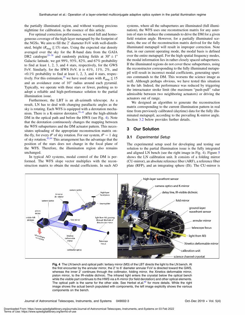
Furthermore, the LBT is an alt-azimuth telescope. As aresult, LN has to deal with changing parallactic angles as thesky is rotating. Each WFS is equipped with a derotation mecha-nism. There is a K-mirror derotator,39–41 after the high-altitudeDM in the optical path and before the HWS (see Fig. 4). Notethat the derotation continuously changes the mapping betweenthe WFS subapertures and the DM actuator pattern. This neces-sitates uploading of the appropriate reconstruction matrix on-the-fly, for every θ° of sky rotation. For our system, θ° ¼ 1 deg

of sky rotation.43,44 This arrangement has the advantage that theposition of the stars does not change in the focal plane ofthe WFS. Therefore, the illumination region also remainsunchanged.

In typical AO systems, modal control of the DM is per-formed. The WFS slope vector multiplies with the recon-struction matrix to obtain the modal coefficients. In such AO

systems, where all the subapertures are illuminated (full illumi-nation), the WFS uses one reconstruction matrix for any aster-ism of stars to deduce the commands to drive the DM for a givenfield rotation angle. However, for a partially illuminated sce-nario, the use of the reconstruction matrix derived for the fullyilluminated metapupil will result in improper correction. Notethat, in our current operating mode, the modal basis is definedover the entire metapupil. For the high spatial frequency modes,the modal information lies in rather closely spaced subapertures.If the illuminated regions do not cover these subapertures, usingthe reconstructor corresponding to the fully illuminated metapu-pil will result in incorrect modal coefficients, generating spuri-ous commands to the DM. This worsens the science image aswell. Although perhaps obvious, we have tested this situationin the lab. Indeed, the performance was reduced by triggeringthe interactuator stroke limit (the maximum “push-pull” valueadmissible between two neighboring actuators) or driving theactuators out of range.

We designed an algorithm to generate the reconstructionmatrix corresponding to the current illumination pattern in realtime from previously calibrated (daytime) data for the fully illu-minated metapupil, according to the prevailing K-mirror angle.Section 3.2 below provides further details.

3 Our Solution

3.1 Experimental Setup

The experimental setup used for developing and testing oursolution to the partial illumination issue is the fully integratedand aligned LN bench (see the right image in Fig. 4). Figure 5shows the LN calibration unit. It consists of a folding mirror(CU-mirror), an absolute reference fiber (ARF), a reference fiberplate (RFP), and an integrating sphere (IS). The CU-mirror is

Fig. 4 The LN bench and optical path: tertiary mirror (M3) of the LBT directs the light to the LN bench. Atthe first encounter by the annular mirror, the 2’ to 6’ diameter annular FoV is directed toward the GWS,whereas the inner 2’ continues through the collimator, folding mirror, the Xinetics deformable mirror,piston mirror, to the IR-visible dichroic. The infrared light enters the cryostat below the optical benchwhile the visible part continues to the HWS via a K-mirror (for field derotation) and other optical elements.The optical path is the same for the other side. See Herbst et.al.42 for more details. While the rightimage shows the actual bench populated with components, the left image explicitly shows the variouscomponents on the bench.




mounted on a precision rotation stage that allows us to direct thecalibration unit light to the HWS. The ARF defines the on-axistelescope beam. The RFP is mounted on a tip-tilt stage, whichcan also move along the three axes. The RFP has 23 fibersmounted to it, defining a set of “stars” in the 2’ FoV. The centralstar is a monomode near-infrared fiber, whereas the reminder aremultimode 200-μm (0”.33 on the sky) fibers fed by visible-wavelength LEDs. The intensities of the fibers can be individu-ally and remotely controlled. We can thus generate definedstellar asterisms and vary their brightness. Note that the RFPis slightly concave, mimicking the curved focal plane of theLBT. The IS is used for flat-fielding.

The fully illuminated metapupil is generated by illuminatingthe eight outermost fibers in the RFP. Each of the fibers is cali-brated for brightness in real, on-sky magnitudes. For calibrationpurposes, the fiber intensity of each of the eight stars is set toRmag ∼ 6. This ensures good SNR at the HWS CCD whileavoiding saturation. The HWS has eight probes (see Fig. 6)that can move in the 2’ FoV to acquire and center on the stars.Using the fiber plate and the HWS probes, it is possible to

calibrate the HWS, create partial illumination test cases, evalu-ate our algorithm, and optimize the high-layer loop.

3.2 Strategy

In order to close the AO loop, we need to have the correctcombinations of the following four matrices:

(1) The modes to command matrix (M2C) is theresponse of the DM to the orthonormal modal base.It has dimensions of (number of actuators × numberof modes). There will be specific actuator valuesdefining each mode across the DM. When multipliedwith the modal coefficient vector, M2C producesthe commands to be sent to the DM. In our case, themodal basis is the Karhunen–Loéve45 (KL) projectedon the DM space, recognizing the Kolmogorov sta-tistics and the actuator positions on the DM.

(2) The interaction matrix (IM) is the response of theWFS to the DM and has dimensions of [(2× numberof subapertures) × number of modes]. There is a rela-tionship between the WFS subapertures and the DMactuators, depending on the binning of the WFSCCD. Each subaperture corresponds to two adjacentrows of the IM, one for each of the orthogonal axes ofthe slope vectors. The information of how much theDM has to change its shape to produce a specificslope measurement is encoded in the IM.

(3) The reconstruction matrix (RM) or the reconstructoris the pseudoinverse of the IM and therefore hasdimensions of [number of modes × (2× number ofsubapertures)]. The modal coefficient vector is theproduct of the measured slope vector and thereconstructor.

(4) The illumination mask (M) is the image that definesthe illuminated subapertures. Without on-chip bin-ning (i.e., binning = 1), the number of subaperturesfor a fully illuminated metapupil is about 616. Thelength of the measured slopes vector is two times

Fig. 5 (a) Calibration unit on the LN bench, consisting of a folding mirror, a reference fiber, a fiber plate,and an IS. (b) Front view of the fiber plate. Some of the fibers are (red) illuminated.

Fig. 6 The eight probes in the HWS can move over the focal plane toacquire the stars in the 2’ FoV. The minimum separation to avoidcollisions corresponds to 20”.




the number of illuminated subapertures. In most AOsystems, this is fixed. However, in our case, the vectorlength varies.

It is essential to incorporate or “register” the correct combi-nation of the M2C, IM, or RM, and M in the loop. In our case,the M2C is always the same, whereas IM∕RM and M varyaccording to the observed target.

In order to determine if a subaperture is well illuminated ornot, we need to know the SNR. Although the major componentsof flexure are compensated by the CCD positioning algorithm,46

there are factors that favor the M created out of SNR threshold-ing over using geometrical arguments. One of the main reasonsis the following. The amount of light actually reaching the detec-tor will vary according to the seeing since the pyramid FoV islimited (to 1”.1 in diameter). If the stellar magnitudes and thecolors mentioned in the catalog are different from the actual val-ues, the seeing variation may actually create differential illumi-nation at the detector. We, therefore, chose an SNR thresholdcriterion that is easy and quick to determine if a subapertureis illuminated or not.

As the first step for identifying the illuminated pixels, weacquire sky background frames (these are in any case neededfor wavefront sensing later). All the probes that have acquiredthe high-layer reference stars are temporarily moved a short dis-tance to their so-called shadow-positions, where the starlight isblocked by the probes and does not reach the HWS CCD. At thispoint, F sky frames are taken. The GWS is in closed-loop whilethe high-layer probes are individually centered (averaging wellover the turbulence, with a precision close to one-tenth of an arcsec) and later while taking the F sky frames. A pixel-by-pixelstandard deviation of these F sky frames forms the noise image.The probes are then sent back to their centered positions andF illuminated frames are taken. A pixelwise median of theseF frames gives the partial illumination image. The SNR imageis then created using the following:

EQ-TARGET;temp:intralink-;e001;63;359SNRimg ¼gPimgffiffiffiffiffiffiffiffiffiffiffiffiffiffiffiffiffiffiffiffiffiffiffiffiffiffiffiffiffiffigPimg þ gðNimgÞ2

q ; (1)

where gPimg is the four-quadrant sum of the partial illumination

image Pimg, and ðNimgÞ2 is the square of the noise image. gPimg isgiven by

EQ-TARGET;temp:intralink-;e002;63;265

gPimg ¼X4

quadrant¼1

ðPimgÞquadrant: (2)

The pixels in the SNRimg with values higher than a giventhreshold will be masked to 1 and others to 0, creating M.Typically, the value of F we use is 1000.

Depending on the HWS CCD binning and the seeing, theright SNR criterion has to be used. We have a look-up table forthis, which is created empirically in open-loop looking to thebehavior in closed-loop. During the observation, we patrol theillumination to take care of the mispositioning of the probe dueto flexures. Note that any partially illuminated mask created bythe SNR threshold criterion will be a subset of the fully illumi-nated mask. Figure 3 illustrates this.

Section 2 explains why we cannot use the same RM as forfull illumination. In our solution, depending on the illuminatedregion, a new IM is extracted from the fully illuminated IM for

the current K-mirror angle. We name the fully illuminated IMthe “mother interaction matrix” (mother-IM) and the reduced,partially illuminated one the “daughter interaction matrix”(daughter-IM). The following subsections present the detailsof the calibration of the mother-IM and the extraction of thedaughter-IM.

3.2.1 Calibrating the mother interaction matrix

Our partial illumination algorithm depends fundamentally on awell-calibrated, fully illuminated, well-conditioned mother-IMfor the given M2C. The condition number describes the sensi-tivity of a function to changes or errors in the measurement data.In other words, the condition number is a proportionality factorin the error. The higher the condition number of a matrix, themore singular or rank deficient is the matrix. For a well-condi-tioned matrix, the noise propagates smoothly over the Eigenmodes, and the condition number will be small.

For the calibration, we use SNR threshold of 20 to identifythe illuminated subapertures. This SNR threshold is for a set ofRmag ∼ 6 “stars” illuminating the full metapupil. After acquiringand centering the eight HWS star probes on the eight fibers inthe outermost ring of the RFP, we measure the actual illumina-tion on the metapupil.

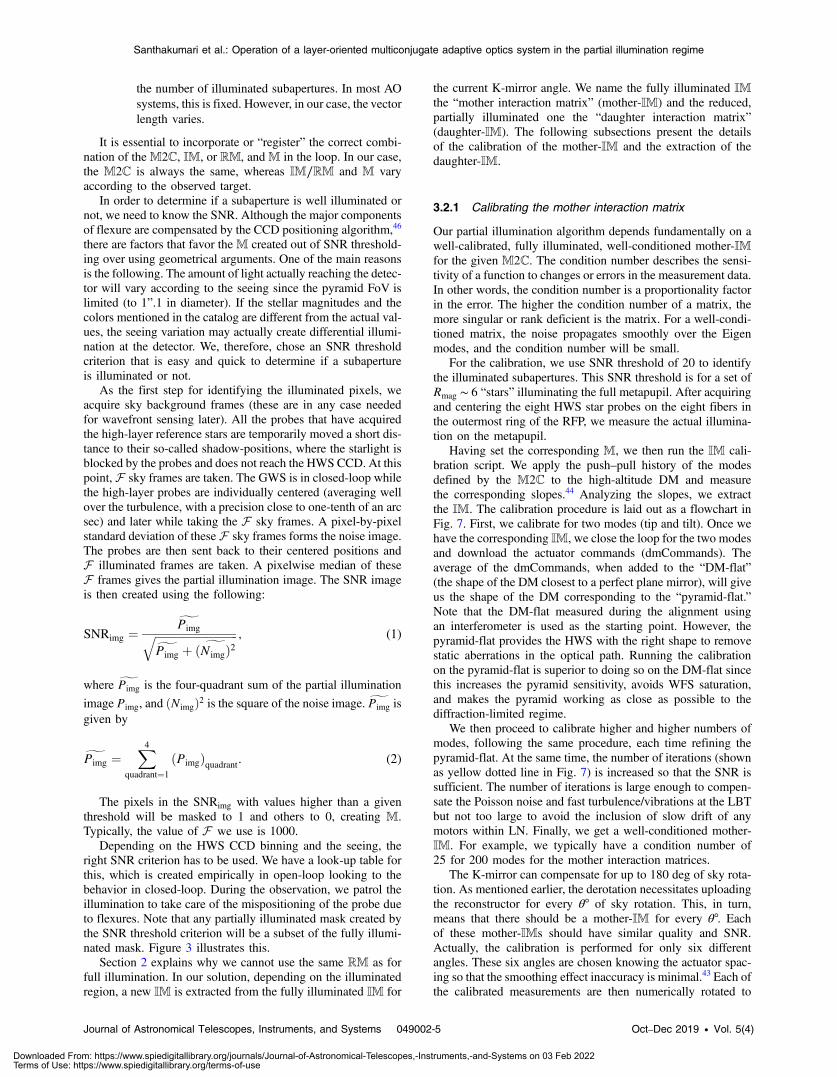
Having set the corresponding M, we then run the IM cali-bration script. We apply the push–pull history of the modesdefined by the M2C to the high-altitude DM and measurethe corresponding slopes.44 Analyzing the slopes, we extractthe IM. The calibration procedure is laid out as a flowchart inFig. 7. First, we calibrate for two modes (tip and tilt). Once wehave the corresponding IM, we close the loop for the two modesand download the actuator commands (dmCommands). Theaverage of the dmCommands, when added to the “DM-flat”(the shape of the DM closest to a perfect plane mirror), will giveus the shape of the DM corresponding to the “pyramid-flat.”Note that the DM-flat measured during the alignment usingan interferometer is used as the starting point. However, thepyramid-flat provides the HWS with the right shape to removestatic aberrations in the optical path. Running the calibrationon the pyramid-flat is superior to doing so on the DM-flat sincethis increases the pyramid sensitivity, avoids WFS saturation,and makes the pyramid working as close as possible to thediffraction-limited regime.

We then proceed to calibrate higher and higher numbers ofmodes, following the same procedure, each time refining thepyramid-flat. At the same time, the number of iterations (shownas yellow dotted line in Fig. 7) is increased so that the SNR issufficient. The number of iterations is large enough to compen-sate the Poisson noise and fast turbulence/vibrations at the LBTbut not too large to avoid the inclusion of slow drift of anymotors within LN. Finally, we get a well-conditioned mother-IM. For example, we typically have a condition number of25 for 200 modes for the mother interaction matrices.

The K-mirror can compensate for up to 180 deg of sky rota-tion. As mentioned earlier, the derotation necessitates uploadingthe reconstructor for every θ° of sky rotation. This, in turn,means that there should be a mother-IM for every θ°. Eachof these mother-IMs should have similar quality and SNR.Actually, the calibration is performed for only six differentangles. These six angles are chosen knowing the actuator spac-ing so that the smoothing effect inaccuracy is minimal.43 Each ofthe calibrated measurements are then numerically rotated to




each integral degree. The average of the six numerically rotatedmeasurements forms the final mother-IM for each angle.

3.2.2 Extracting the daughter interaction matrix

As described in Sec. 3.2 above, there will be a uniqueM for eachasterism. It is essential to have the correct IMmatching theM toclose the loop. Calibrating a new IM for each asterism wouldconsume a lot of observing time. To avoid this, we came up withthe following algorithm.

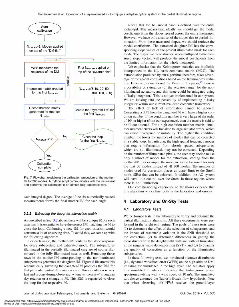
For each angle, the mother-IM contains the slope responsefor every subaperture and calibrated mode. The subaperturesilluminated in the partially illuminated case are of course illu-minated in the fully illuminated case as well. Removing thoserows in the mother-IM corresponding to the nonilluminatedsubapertures generates the daughter-IM. Figure 8 illustrates thisschematically. Inverting the daughter-IM produces the RM forthat particular partial illumination case. This calculation is veryfast and is done during observing, whenever there is θ° change insky rotation or a change in M. This RM is registered to closethe loop for the respective M.

Recall that the KL modal base is defined over the entiremetapupil. This means that, ideally, we should get the modalcoefficients from the slopes spread across the entire metapupil.However, we have only a subset of the slopes due to partial illu-mination. From these measured slopes, we should retrieve themodal coefficients. The extracted daughter-IM has the corre-sponding slope values of the present illuminated mask for eachmode. The respective reconstructor, when multiplied to the mea-sured slope vector, will produce the modal coefficients fromthe limited information for the whole metapupil.

We emphasize that the Kolmogorov statistics are implicitlyincorporated in the KL basis command matrix (M2C). Theextrapolation produced by our algorithm, therefore, takes advan-tage of the spatial correlations based on the Kolmogorov statis-tics. However, as mentioned by Véran in his paper,47 there isa possibility of saturation (of the actuator range) for the non-illuminated actuators, and this issue could be mitigated usinga “leaky integrator.” This is not yet implemented in our system.We are looking into the possibility of implementing a leakyintegrator within our current real-time computer framework.

The effect of lack of information cannot be ignored.Generating a RM from the daughter-IM will have a higher con-dition number. If the condition number is very large of the orderof 103 or higher (from our experience), then the matrix is said tobe ill-conditioned. For a high condition number matrix, smallmeasurement errors will translate to large actuator errors, whichcan cause divergence or instability. The higher the conditionnumber, the lower the number of modes that can be correctedin a stable loop. In particular, the high spatial frequency modesthat require information from closely spaced subapertures,which are not illuminated, may not be corrected. Dependingon the number of illuminated pixels, the user may decide to useonly a subset of modes for the extraction, starting from themother-IM. For example, the user can decide to correct for onlythe first 50 modes instead of all 200 modes. The number ofmodes used for correction places an upper limit to the Strehlratios (SRs) that can be achieved. In addition, the AO systemwill have little control over the Strehl in those regions wherethere is no illumination.

Our commissioning experience so far shows evidence thatthis algorithm works fine, both in the laboratory and on-sky.

4 Laboratory and On-Sky Tests

4.1 Laboratory Tests

We performed tests in the laboratory to verify and optimize thepartial illumination algorithm. All these experiments were per-formed in the bright-end regime. The goals of these tests were(1) to determine the effect of the selection of subapertures andthe impact of reasonable variation in the SNR threshold onthe correction, (2) to determine differences in getting thereconstructor from the daughter-IM with and without truncationin the singular value decomposition (SVD), and (3) to quantifythe quality of correction as a function of the illuminatedsubapertures.

In these following tests, we introduced a known disturbance[i.e., dynamic wavefront error (WFE)] on the high-altitude DM,imitating the turbulence in the high layer. The actuators applythis simulated turbulence following the Kolmogorov powerspectrum evolving with a wind speed of 10 m/s. The simulatedturbulence assumed the Taylor’s frozen flow hypothesis. Notethat when observing, the HWS receives the ground-layer

Fig. 7 Flowchart explaining the calibration procedure of the mother-IM for 200 modes. A Python script communicates with the instrumentand performs the calibration in an almost fully automatic way.




corrected wavefront. We selected a disturbance with a root meansquare (RMS) WFE of ∼550 nm after the ground-layer correc-tion. Later, we obtained similar residual RMS WFE valuesafter the ground-layer correction on good seeing conditions(0”.7 in V-band).

4.1.1 Impact of reasonable variation in the SNR thresholdon the correction

The SNR threshold will define if a subaperture within the meta-pupil is illuminated or not. We wanted to verify how sensitivethe quality of the correction is to the SNR threshold. In particu-lar, the impact of losing the outermost subapertures is due to theSNR threshold value for a bright asterism. This verification isnecessary since the quality of the correction can otherwise varya lot, and the stability of the loop may be affected.

For this test, we considered two cases: (1) eight stars aster-ism, corresponding to full illumination and (2) three stars aster-ism, corresponding to a partial illumination scenario. For bothcases, all of the stars were of Rmag ∼ 6 equivalent brightness.A dynamic WFE of 536 nm was applied to the high-altitudeDM to check the correction performance.

Each calibrated mode has its own gain, and together, thesevalues form the gain vector. Typically, we split the modes intothree groups—tip and tilt (modes 1 and 2), modes from 3 to 50,and modes higher than 50. Each of these groups were given anindividual constant gain value while closing the loop. For eachSNR threshold value trial, we optimized the gain vector to pro-duce the best, stable correction.

The quality of correction is quantified by the residual RMSmodal coefficients and by the residual RMS WFE. The RMSmodal coefficients can be estimated in two ways: (a) directlyfrom the residual wavefront slopes (by multiplying with theRM) and (2) from the dmCommands computed over the full

metapupil (by multiplying with the M2C). We used the secondone as it provides the residual over the entire metapupil and notjust the illuminated part. The RMS WFE is evaluated from themodal coefficients, as the quadrature sum of the RMS modalcoefficients.

Different SNR threshold values result in slightly differentmasks, differing, of course, in the number of subaperturesilluminated. The reasonable SNR threshold range was definedsuch that the geometrical projection of the stars on the HWSCCD and that on the sky are very close, and only the subaper-tures at the edges of the pupils were affected. In the full illumi-nation case, the SNR threshold range was 10 to 25, for whichthe number of selected subapertures ranged from 616 to 588.Similarly, for the partial illumination case, the SNR thresholdrange was 5 to 20. The corresponding number of subaperturesranged from 528 to 484.

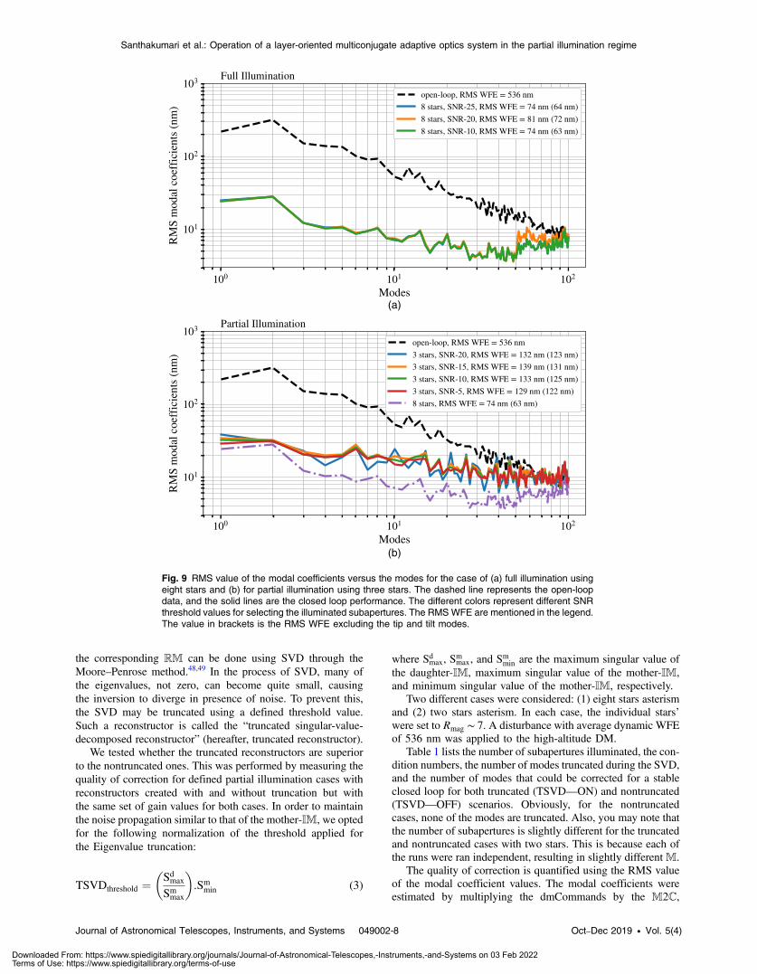
The effect of the different SNR thresholds on the correctionfor the two cases appears in Fig. 9, where the RMS value ofthe modal coefficients is plotted against the modes. The blackdashed line is the open-loop with an RMS WFE of 536 nm.The solid lines, in different colors, represent the performancefor different reasonable SNR threshold values. For both the fulland partial illumination cases, there is a clear improvement,independent of the SNR threshold, reducing the WFE to ∼65and 125 nm, respectively. This means that for the bright-endregimes, the correction is not sensitive on the actual SNR thresh-old value used, as long as it is within a reasonable range, for bothfull and partial illumination scenarios.

4.1.2 Partial illumination reconstructor with and withouttruncation in the singular value decomposition

Section 3.2.2 describes the extraction of the daughter-IM fromthe respective mother-IM. The inverse of the daughter-IM to get

Fig. 8 A schematic diagram explaining the extraction of the daughter-IM from the mother-IM. On the left,the fully illuminated metapupil and the corresponding IM can be seen. On the right, the partiallyilluminated metapupil appears along with the daughter-IM extracted out of the mother-IM.




the corresponding RM can be done using SVD through theMoore–Penrose method.48,49 In the process of SVD, many ofthe eigenvalues, not zero, can become quite small, causingthe inversion to diverge in presence of noise. To prevent this,the SVD may be truncated using a defined threshold value.Such a reconstructor is called the “truncated singular-value-decomposed reconstructor” (hereafter, truncated reconstructor).

We tested whether the truncated reconstructors are superiorto the nontruncated ones. This was performed by measuring thequality of correction for defined partial illumination cases withreconstructors created with and without truncation but withthe same set of gain values for both cases. In order to maintainthe noise propagation similar to that of the mother-IM, we optedfor the following normalization of the threshold applied forthe Eigenvalue truncation:

EQ-TARGET;temp:intralink-;e003;63;105TSVDthreshold ¼�Sdmax

Smmax

�:Smmin (3)

where Sdmax, Smmax, and Smmin are the maximum singular value ofthe daughter-IM, maximum singular value of the mother-IM,and minimum singular value of the mother-IM, respectively.

Two different cases were considered: (1) eight stars asterismand (2) two stars asterism. In each case, the individual stars’were set to Rmag ∼ 7. A disturbance with average dynamic WFEof 536 nm was applied to the high-altitude DM.

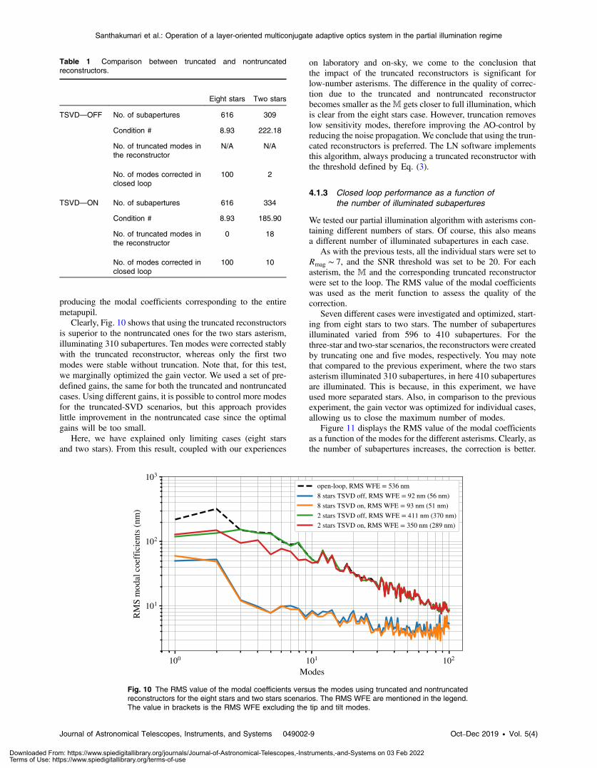
Table 1 lists the number of subapertures illuminated, the con-dition numbers, the number of modes truncated during the SVD,and the number of modes that could be corrected for a stableclosed loop for both truncated (TSVD—ON) and nontruncated(TSVD—OFF) scenarios. Obviously, for the nontruncatedcases, none of the modes are truncated. Also, you may note thatthe number of subapertures is slightly different for the truncatedand nontruncated cases with two stars. This is because each ofthe runs were ran independent, resulting in slightly different M.

The quality of correction is quantified using the RMS valueof the modal coefficient values. The modal coefficients wereestimated by multiplying the dmCommands by the M2C,

(a)

(b)

Fig. 9 RMS value of the modal coefficients versus the modes for the case of (a) full illumination usingeight stars and (b) for partial illumination using three stars. The dashed line represents the open-loopdata, and the solid lines are the closed loop performance. The different colors represent different SNRthreshold values for selecting the illuminated subapertures. The RMSWFE are mentioned in the legend.The value in brackets is the RMS WFE excluding the tip and tilt modes.




producing the modal coefficients corresponding to the entiremetapupil.

Clearly, Fig. 10 shows that using the truncated reconstructorsis superior to the nontruncated ones for the two stars asterism,illuminating 310 subapertures. Ten modes were corrected stablywith the truncated reconstructor, whereas only the first twomodes were stable without truncation. Note that, for this test,we marginally optimized the gain vector. We used a set of pre-defined gains, the same for both the truncated and nontruncatedcases. Using different gains, it is possible to control more modesfor the truncated-SVD scenarios, but this approach provideslittle improvement in the nontruncated case since the optimalgains will be too small.

Here, we have explained only limiting cases (eight starsand two stars). From this result, coupled with our experiences

on laboratory and on-sky, we come to the conclusion thatthe impact of the truncated reconstructors is significant forlow-number asterisms. The difference in the quality of correc-tion due to the truncated and nontruncated reconstructorbecomes smaller as theM gets closer to full illumination, whichis clear from the eight stars case. However, truncation removeslow sensitivity modes, therefore improving the AO-control byreducing the noise propagation. We conclude that using the trun-cated reconstructors is preferred. The LN software implementsthis algorithm, always producing a truncated reconstructor withthe threshold defined by Eq. (3).

4.1.3 Closed loop performance as a function ofthe number of illuminated subapertures

We tested our partial illumination algorithm with asterisms con-taining different numbers of stars. Of course, this also meansa different number of illuminated subapertures in each case.

As with the previous tests, all the individual stars were set toRmag ∼ 7, and the SNR threshold was set to be 20. For eachasterism, the M and the corresponding truncated reconstructorwere set to the loop. The RMS value of the modal coefficientswas used as the merit function to assess the quality of thecorrection.

Seven different cases were investigated and optimized, start-ing from eight stars to two stars. The number of subaperturesilluminated varied from 596 to 410 subapertures. For thethree-star and two-star scenarios, the reconstructors were createdby truncating one and five modes, respectively. You may notethat compared to the previous experiment, where the two starsasterism illuminated 310 subapertures, in here 410 subaperturesare illuminated. This is because, in this experiment, we haveused more separated stars. Also, in comparison to the previousexperiment, the gain vector was optimized for individual cases,allowing us to close the maximum number of modes.

Figure 11 displays the RMS value of the modal coefficientsas a function of the modes for the different asterisms. Clearly, asthe number of subapertures increases, the correction is better.

Table 1 Comparison between truncated and nontruncatedreconstructors.

Eight stars Two stars

TSVD—OFF No. of subapertures 616 309

Condition # 8.93 222.18

No. of truncated modes inthe reconstructor

N/A N/A

No. of modes corrected inclosed loop

100 2

TSVD—ON No. of subapertures 616 334

Condition # 8.93 185.90

No. of truncated modes inthe reconstructor

0 18

No. of modes corrected inclosed loop

100 10

Fig. 10 The RMS value of the modal coefficients versus the modes using truncated and nontruncatedreconstructors for the eight stars and two stars scenarios. The RMS WFE are mentioned in the legend.The value in brackets is the RMS WFE excluding the tip and tilt modes.




However, clustering and jump of the performance may be notedfrom the plot. This is because the modal basis is defined over theentire metapupil, as mentioned earlier. Some specific modesmay not be adequately seen by the WFS, depending on the non-illuminated regions of the metapupil. Controlling these modes ispossible with lower gain values. For this experiment, we havenot individually tuned the gain values for individual modes.The gain values are split into three sets, as mentioned earlier,optimizing to produce the best performance for each asterismscenario. Note, however, that within each set, the gain value hasthe same scalar value. We are able to set relatively higher gainvalues and have the loop stable when theM is closer to full, evenfor the higher order modes. In contrast, for the two and threestars asterisms, with correspondingly fewer illuminated subaper-tures, we could only set relatively low gain values for the higherorder modes (modes > 50).

In contrast to Fig. 10, note that all 100 modes were correctedfor the two stars asterism as well. This is due to the fact that wecarefully optimized the gain vector, thereby allowing a stableloop. In addition, in this case, the two stars were illuminatingdifferent regions of the metapupil and illuminating more numberof subapertures. Although the correction is relatively poor forthe two stars asterism, the fact that there is decent correction,which confirms that the partial illumination algorithm works.

4.2 On-Sky Tests

The final assessment of the performances of any AO systemshould come from on-sky testing. We have tested our implemen-tation of the partial illumination solution in this way during LNcommissioning. The goals were to verify the software compat-ibility of our solution with the rest of the LN MCAO system, totest the creation of the partial illumination mask, to verify theextraction of the daughter-IM and the uploading of the truncatedreconstructor for the current K-mirror angle, and to check theHWS closed-loop performance with partial illumination.

During the second (June 2017) and third (January 2018) LNcommissioning runs, we demonstrated the basic operation andfunctionality of the partial illumination code. This includedthe software compatibility of our solution with the high-layer

wavefront sensing service and LNMCAO software architecture,in general, creation of the partial illumination, and the extractionof the daughter-IM.

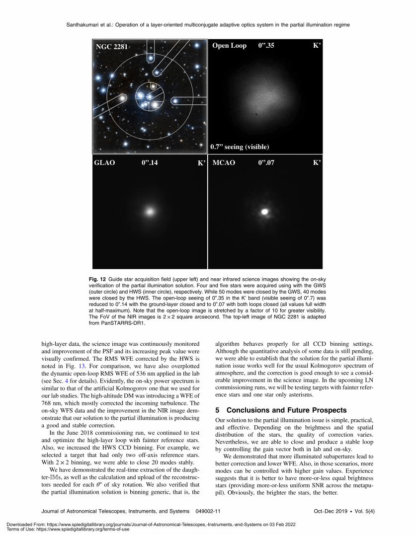
During the fourth commissioning run (April 2018), we suc-cessfully tested the CCD tracking algorithm that maintains theoptical conjugation while observing. Also, both ground- andhigh-layer loops were stably closed, providing considerableimprovement of the science image. One of the science targetswas NGC 2281. A total of nine stars were acquired to measurethe atmospheric turbulence. Figure 12 shows the asterism ofstars and the processed NIR images of the central star. Theground-layer was closed using 50 modes. The ground-layeradaptive optics (GLAO) image measured a SR of ∼7.7%(K-band). 497 out of 616 subapertures within the metapupilwere illuminated using five stars acquired by the HWS. Notethat the central star, NGC 2281, was also one of the high-layerreference stars. We were able to close the high-layer loop stablywith 40 modes, starting from a stable, ground-layer correctedwavefront. We measured the SR of the MCAO image to be∼22% (K-band). The peak of the PSF (in K-band) jumpedby a factor of ∼2.8 from GLAO to MCAO.

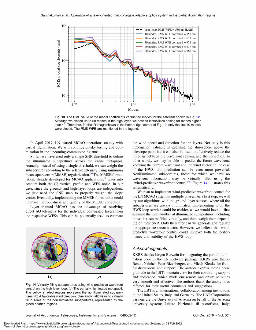
For estimating the on-sky, partial illumination performance,we downloaded a set of dmCommands each time that we closedthe high-layer loop with different number of modes, each timeoptimizing the gain vector. Note that these data were taken veryclosely spaced in time, and we assume the atmosphere remainedmore or less the same then. From the dmCommands, we esti-mated the modal coefficients. Figure 13 shows the RMS value ofthe modal coefficients as a function of the modes for the sametarget. We overplotted each sets of data to check if there isany performance degradation while closing higher number ofmodes. As we close higher number of modes, starting from10 to 50, the low-order modes are always corrected by thesimilar amount. There is no degradation in performance in thelow-order modes while the high-spatial frequency modes arealso corrected.

We remind that the acquisition of the NIR data (Fig. 12) andthe WFS data used to make the plot in Fig. 13 were taken simul-taneously or in very closely spaced time. While acquiring the

Fig. 11 The RMS value of the modal coefficients versus themodes for varying number of stars. The RMSWFE arementioned in the legend. The value in brackets is the RMSWFE excluding the tip and tilt modes.




high-layer data, the science image was continuously monitoredand improvement of the PSF and its increasing peak value werevisually confirmed. The RMS WFE corrected by the HWS isnoted in Fig. 13. For comparison, we have also overplottedthe dynamic open-loop RMS WFE of 536 nm applied in the lab(see Sec. 4 for details). Evidently, the on-sky power spectrum issimilar to that of the artificial Kolmogorov one that we used forour lab studies. The high-altitude DMwas introducing aWFE of768 nm, which mostly corrected the incoming turbulence. Theon-sky WFS data and the improvement in the NIR image dem-onstrate that our solution to the partial illumination is producinga good and stable correction.

In the June 2018 commissioning run, we continued to testand optimize the high-layer loop with fainter reference stars.Also, we increased the HWS CCD binning. For example, weselected a target that had only two off-axis reference stars.With 2 × 2 binning, we were able to close 20 modes stably.

We have demonstrated the real-time extraction of the daugh-ter-IMs, as well as the calculation and upload of the reconstruc-tors needed for each θ° of sky rotation. We also verified thatthe partial illumination solution is binning generic, that is, the

algorithm behaves properly for all CCD binning settings.Although the quantitative analysis of some data is still pending,we were able to establish that the solution for the partial illumi-nation issue works well for the usual Kolmogorov spectrum ofatmosphere, and the correction is good enough to see a consid-erable improvement in the science image. In the upcoming LNcommissioning runs, we will be testing targets with fainter refer-ence stars and one star only asterisms.

5 Conclusions and Future ProspectsOur solution to the partial illumination issue is simple, practical,and effective. Depending on the brightness and the spatialdistribution of the stars, the quality of correction varies.Nevertheless, we are able to close and produce a stable loopby controlling the gain vector both in lab and on-sky.

We demonstrated that more illuminated subapertures lead tobetter correction and lower WFE. Also, in those scenarios, moremodes can be controlled with higher gain values. Experiencesuggests that it is better to have more-or-less equal brightnessstars (providing more-or-less uniform SNR across the metapu-pil). Obviously, the brighter the stars, the better.

Fig. 12 Guide star acquisition field (upper left) and near infrared science images showing the on-skyverification of the partial illumination solution. Four and five stars were acquired using with the GWS(outer circle) and HWS (inner circle), respectively. While 50 modes were closed by the GWS, 40 modeswere closed by the HWS. The open-loop seeing of 0”.35 in the K’ band (visible seeing of 0”.7) wasreduced to 0”.14 with the ground-layer closed and to 0”.07 with both loops closed (all values full widthat half-maximum). Note that the open-loop image is stretched by a factor of 10 for greater visibility.The FoV of the NIR images is 2 × 2 square arcsecond. The top-left image of NGC 2281 is adaptedfrom PanSTARRS-DR1.




In April 2017, LN started MCAO operations on-sky withpartial illumination. We will continue on-sky testing and opti-mization in the upcoming commissioning runs.

So far, we have used only a single SNR threshold to definethe illuminated subapertures across the entire metapupil.Actually, instead of using a single threshold, we can weight thesubapertures according to the relative intensity using minimummean square error (MMSE) regularization.50 The MMSE formu-lation, already developed for MCAO applications,51 takes intoaccount both the C2

n vertical profile and WFS noise. In ourcase, since the ground- and high-layer loops are independent,we just need the SNR map to properly weight the slopevector. Eventually, implementing the MMSE formulation couldimprove the robustness and quality of the MCAO correction.

Layer-oriented MCAO has the advantage of receivingdirect AO telemetry for the individual conjugated layers fromthe respective WFSs. This can be potentially used to estimate

the wind speed and direction for the layers. Not only is thisinformation valuable in profiling the atmosphere above thetelescope pupil but it can also be used to effectively reduce thetime-lag between the wavefront sensing and the correction. Inother words, we may be able to predict the future wavefront,knowing the current wavefront and the wind vector. In the caseof the HWS, this prediction can be even more powerful.Nonilluminated subapertures, those for which we have nowavefront information, may be virtually filled using the“wind-predictive wavefront control.”34 Figure 14 illustrates thisschematically.

We plan to implement wind-predictive wavefront control forthe LNMCAO system in multiple phases. As a first step, we willtry our algorithms with the ground-layer sensors, where all thesubapertures are always illuminated. Implementing it on theHWS loop service could be trickier, as we would have to firstestimate the total number of illuminated subapertures, includingthose that can be filled virtually, and then, weigh them depend-ing on their SNR. Only thereafter can we generate and registerthe appropriate reconstructor. However, we believe that wind-predictive wavefront control could improve both the perfor-mance and stability of the HWS loop.

AcknowledgmentsKKRS thanks Jürgen Berwein for integrating the partial illumi-nation code to the LN software package. KKRS also thanksBenoit Neichel, Peter Bizenberger, and Micah Klettke for fruit-ful discussions and support. The authors express their sinceregratitude to the LBT mountain crew for their continuing supportand dedication, which made our remote and onsite activitiesvery smooth and effective. The authors thank the anonymousreferees for their useful comments and suggestions.

The LBT is an international collaboration among institutionsin the United States, Italy, and Germany. The LBT Corporationpartners are the University of Arizona on behalf of the Arizonauniversity system; Istituto Nazionale di Astrofisica, Italy;

Fig. 14 Virtually filling subapertures using wind-predictive wavefrontcontrol on the high layer loop. (a) The partially illuminated metapupil.The yellow shaded regions represent the nonilluminated subaper-tures. (b) A favorable wind direction (blue arrow) allows us to virtuallyfill in some of the nonilluminated subapertures, represented by thegreen shaded regions.

Fig. 13 The RMS value of the modal coefficients versus the modes for the asterism shown in Fig. 12.Although we closed up to 50 modes in the high layer, we noticed instabilities arising for modes higherthan 40. Therefore, for the IR image shown in the bottom-right corner of Fig. 12, only the first 40 modeswere closed. The RMS WFE are mentioned in the legend.




LBT Beteiligungsgesellschaft, Germany, representing the MaxPlanck Society, the Astrophysical Institute Potsdam, andHeidelberg University; The Ohio State University; TheResearch Corporation, on behalf of the University of NotreDame, University of Minnesota, and University of Virginia.

This work has made use of data from the European SpaceAgency (ESA) mission Gaia,52 processed by the Gaia DataProcessing and Analysis Consortium (DPAC).53 Funding for theDPAC has been provided by national institutions, in particular,the institutions participating in the Gaia Multilateral Agreement.

This research made use of Astropy, a community-developedcore Python package for Astronomy, and the IPython package.Furthermore, the author used the following python packagesextensively within the partial illumination code: NumPy,Matplotlib, and SciPy. This research has made use of NASA’sAstrophysics Data System Bibliographic Services.

References1. J. M. Beckers, “Increasing the size of the isoplanatic patch with multi-

conjugate adaptive optics,” in Eur. South. Obs. Conf. and WorkshopProc., M.-H. Ulrich, Ed., Vol. 30, p. 693 (1988).

2. J. M. Beckers, “Detailed compensation of atmospheric seeing usingmulticonjugate adaptive optics,” Proc. SPIE 1114, 215–217 (1989).

3. R. Ragazzoni, E. Marchetti, and F. Rigaut, “Modal tomography foradaptive optics,” Astron. Astrophys. 342, L53–L56 (1999).

4. R. Ragazzoni, E. Marchetti, and G. Valente, “Adaptive-optics correc-tions available for the whole sky,” Nature 403, 54–56 (2000).

5. E. Marchetti et al., “MAD the ESO multi-conjugate adaptive opticsdemonstrator,” Proc. SPIE 4839, 317–328 (2003).

6. E. Marchetti et al., “MAD: practical implementation of MCAO con-cepts,” C. R. Phys. 6, 1118–1128 (2005).

7. E. Marchetti, “MAD upgrade proposal: concept & correction perfor-mance,” in MAD and Beyond Workshop, ESO, Garching (2009).

8. S. Esposito et al., “AOF upgrade for VLT UT4: an 8 m class HST fromground,” Proc. SPIE 9909, 99093U (2016).

9. E. Diolaiti et al., “MAORY: adaptive optics module for the E-ELT,”Proc. SPIE 9909, 99092D (2016).

10. G. Herriot et al., “NFIRAOS: first facility AO system for the ThirtyMeter Telescope,” Proc. SPIE 9148, 914810 (2014).

11. F. Rigaut and B. Neichel, “Multiconjugate adaptive optics forastronomy,” Annu. Rev. Astron. Astrophys. 56(1), 277–314 (2018).

12. F. Rigaut et al., “Gemini multiconjugate adaptive optics system review -I. Design, trade-offs and integration,” Mon. Not. R. Astron. Soc. 437,2361–2375 (2014).

13. B. Neichel et al., “Gemini multiconjugate adaptive optics systemreview - II. Commissioning, operation and overall performance,”Mon. Not. R. Astron. Soc. 440, 1002–1019 (2014).

14. T. M. Herbst et al., “The LINC NIRVANA multi-conjugate adaptiveoptics imager,” in preparation (2019).

15. T. M. Herbst et al., “LINC-NIRVANA: a Fizeau beam combiner forthe large binocular telescope,” Proc. SPIE 4838, 456–465 (2003).

16. T. M. Herbst et al., “Novel adaptive optics on the pathway to ELTs:MCAO with LINC-NIRVANA on LBT,” in 2nd Int. Conf. Adapt.Opt. for Extrem. Large Telesc., p. 20, (2011).

17. T. M. Herbst et al., “Installation and commissioning of the LINC-NIRVANA near-infrared MCAO imager on LBT,” Proc. SPIE 10702,107020U (2018).

18. M. Tallon, R. Foy, and J. Vermin, “3-D wavefront sensing for multicon-jugate adaptive optics,” in Eur. South. Obs. Conf. and Workshop Proc.,Vol. 42, p. 517 (1992).

19. R. Ragazzoni, J. Farinato, and E. Marchetti, “Adaptive optics for 100-m-class telescopes: new challenges require new solutions,” Proc. SPIE4007, 1076–1087 (2000).

20. C. Arcidiacono et al., “Toward the first light of the layer oriented wave-front sensor for MAD,” Mem. Soc. Astron. Ital. 78, 708 (2007).

21. T. M. Herbst et al., “Commissioning multi-conjugate adaptive opticswith LINC-NIRVANA on LBT,” Proc. SPIE 10703, 107030B(2018).

22. R. Ragazzoni, “Pupil plane wavefront sensing with an oscillatingprism,” J. Mod. Opt. 43, 289–293 (1996).

23. R. Ragazzoni et al., “Multiple field of view layer-oriented adaptiveoptics. Nearly whole sky coverage on 8 m class telescopes and beyond,”Astron. Astrophys. 396, 731–744 (2002).

24. J. Farinato et al., “The multiple field of view layer oriented wavefrontsensing system of LINC-NIRVANA: two arcminutes of corrected fieldusing solely natural guide stars,” Proc. SPIE 7015, 70155J (2008).

25. C. Arcidiacono et al., “Sky coverage for layer-oriented MCAO:a detailed analytical and numerical study,” Proc. SPIE 5490, 563–573(2004).

26. A. Tokovinin and E. Viard, “Limiting precision of tomographic phaseestimation,” J. Opt. Soc. Am. A 18, 873–882 (2001).

27. R. Ragazzoni et al., “Multiple field of view layer oriented,” in Eur.South. Obs. Conf. and Workshop Proc., Vol. 58, p. 75 (2002).

28. A. Wirth et al., “Deformable mirror technologies at AOA Xinetics,”Proc. SPIE 8780, 87800M (2013).

29. R. Ragazzoni and J. Farinato, “Sensitivity of a pyramidic wave frontsensor in closed loop adaptive optics,” Astron. Astrophys. 350,L23–L26 (1999).

30. V. Viotto et al., “Expected gain in the pyramid wavefront sensor withlimited Strehl ratio,” Astron. Astrophys. 593, A100 (2016).

31. C. Vérinaud et al., “Layer oriented multi-conjugate adaptive opticssystems: performance analysis by numerical simulations,” Proc. SPIE4839, 524–535 (2003).

32. T. Bertram et al., “Wavefront sensing in a partially illuminated, rotatingpupil,” Proc. SPIE 9148, 91485M (2014).

33. K. K. R. Santhakumari et al., “Solving the MCAO partial illuminationissue and laboratory results,” Proc. SPIE 9909, 99096M (2016).

34. K. K. R. Santhakumari et al., “On-sky verification of a solution tothe MCAO partial illumination issue and wind-predictive wavefrontcontrol,” Proc. SPIE 10703, 107035L (2018).

35. F. Arenou et al., “Gaia data release 2. Catalogue validation,” Astron.Astrophys. 616, A17 (2018).

36. A. G. A. Brown et al., “Gaia data release 2. Summary of the contentsand survey properties,” Astron. Astrophys. 616, A1 (2018).

37. T. Prusti et al., “The Gaia mission,” Astron. Astrophys. 595, A1 (2016).38. M. Riello et al., “Gaia Data Release 2. Processing of the photometric

data,” Astron. Astrophys. 616, 16–24 (2018).39. D. S. Durie, “A compact derotator design,” Opt. Eng. 13, 119 (1974).40. A. Brunelli et al., “Tips and tricks for aligning an image derotator,”

Proc. SPIE 8446, 84464L (2012).41. J. Moreno-Ventas et al., “Optical integration and verification of

LINC-NIRVANA,” Proc. SPIE 9147, 91473V (2014).42. T. M. Herbst et al., “MCAO with LINC-NIRVANA at LBT: preparing

for first light,” Proc. SPIE 9909, 99092U (2016).43. C. Arcidiacono et al., “Numerical control matrix rotation for the LINC-

NIRVANA multiconjugate adaptive optics system,” Proc. SPIE 7736,77364J (2010).

44. C. Arcidiacono et al., “The calibration procedure of the LINC-NIRVANA ground and high layer WFS,” Proc. SPIE 10703, 107034R(2018).

45. J. W. Hardy, “Adaptive Optics for Astronomical Telescopes,” Phys.Today 53(4), 69 (1998).

46. M. Klettke et al., “CCD tracking for gravity flexure compensation onLINC NIRVANA,” in preparation (2019).

47. J.-P. Véran, “Control of the unilluminated deformable mirror actuatorsin an altitude-conjugated adaptive optics system,” J. Opt. Soc. Am. A 17,1325–1332 (2000).

48. E. H. Moore, “On the reciprocal of the general algebraic matrix,” Bull.Am. Math. Soc. 26, 394–395 (1920).

49. R. Penrose, “A generalized inverse for matrices,” Math. Proc.Cambridge Philos. Soc. 51(3), 406–413 (1955).

50. B. L. Ellerbroek, “First-order performance evaluation of adaptive-opticssystems for atmospheric-turbulence compensation in extended-field-of-view astronomical telescopes,” J. Opt. Soc. Am. A 11, 783–805 (1994).

51. T. Fusco et al., “Optimal wave-front reconstruction strategies formulticonjugate adaptive optics,” J. Opt. Soc. Am. A 18, 2527–2538(2001).

52. European Space Agency, https://www.cosmos.esa.int/gaia (2019).53. European Space Agency, https://www.cosmos.esa.int/web/gaia/dpac/

consortium (2019).




https://doi.org/10.1117/12.960826

https://doi.org/10.1038/47425

https://doi.org/10.1117/12.458859

https://doi.org/10.1016/j.crhy.2005.11.002

https://doi.org/10.1117/12.2234737

https://doi.org/10.1117/12.2234585

https://doi.org/10.1117/12.2055525

https://doi.org/10.1146/annurev-astro-091916-055320

https://doi.org/10.1093/mnras/stt2054

https://doi.org/10.1093/mnras/stu403

https://doi.org/10.1117/12.458876

https://doi.org/10.1117/12.2313368

https://doi.org/10.1117/12.390313

https://doi.org/10.1117/12.2313421

https://doi.org/10.1080/09500349608232742

https://doi.org/10.1051/0004-6361:20021406

https://doi.org/10.1117/12.790401

https://doi.org/10.1117/12.551839

https://doi.org/10.1364/JOSAA.18.000873

https://doi.org/10.1117/12.2018031

https://doi.org/10.1051/0004-6361/201528023

https://doi.org/10.1117/12.458965

https://doi.org/10.1117/12.2057384

https://doi.org/10.1117/12.2230683

https://doi.org/10.1117/12.2313235

https://doi.org/10.1051/0004-6361/201833234

https://doi.org/10.1051/0004-6361/201833234

https://doi.org/10.1051/0004-6361/201833051

https://doi.org/10.1051/0004-6361/201629272

https://doi.org/10.1051/0004-6361/201832712

https://doi.org/10.1117/12.7971671

https://doi.org/10.1117/12.926884

https://doi.org/10.1117/12.2057456

https://doi.org/10.1117/12.2232596

https://doi.org/10.1117/12.857347

https://doi.org/10.1117/12.2313152

https://doi.org/10.1063/1.883053

https://doi.org/10.1063/1.883053


https://doi.org/10.1017/S0305004100030401

https://doi.org/10.1017/S0305004100030401



https://www.cosmos.esa.int/gaia




https://www.cosmos.esa.int/web/gaia/dpac/consortium





Kalyan Kumar Radhakrishnan Santhakumari is a postdoctoral fel-low at the INAF-Astronomical Observatory of Padova, Italy. In 2017,he obtained a PhD degree in astronomy and astrophysics fromRuprecht-Karls-Universität Heidelberg, Germany, working on theadaptive optics system of the LINC-NIRVANA instrument at theMax Planck Institute for Astronomy, Heidelberg. He has experienceworking on the AO calibration strategies, commissioning AO systems,and presently, contributing to the various adaptive optics projects(LINC-NIRVANA, INGOT, MAVIS, and SHARK-NIR).

Carmelo Arcidiacono received the PhD in astronomy in 2005,became a staff researcher at the INAF on 2011, and is currently work-ing at the INAF-Astronomical Observatory of Padova. Since 2001, hehas been contributing to the development of astronomical instrumen-tation. His primary expertise is concerning adaptive optics, focusingon numerical simulations, laboratory testing, instrument commission-ing, data analysis, and science targets definition. He is the instrumentscientist of MAORY (ELT) and leads the Science Operation WorkingGroup.

Thomas Bertram received his PhD in physics from the University ofCologne, Germany, in 2007. In 2008, he joined the Max PlanckInstitute for Astronomy in Heidelberg, Germany, where he developsinstrumentation and adaptive optics systems for professional ground-based astronomical observatories. He is the system engineer forLINC-NIRVANA, and since 2016, the single conjugate adaptive opticssystem lead for METIS, the mid-infrared instrument for the ExtremelyLarge Telescope.

Florian Briegel received his master of computer science fromKarlsruhe Institute of Technology (former Technische UniversitätKarlsruhe) in 1992. In 1998, he joined the Max Planck Institute forAstronomy (MPIA) in Heidelberg, Germany, where he developsinstrumentation control and adaptive optics software for professionalground-based astronomical observatories. Since 2009, he is the headof the software development department at MPIA.

Thomas M. Herbst is a senior staff astronomer and research groupleader at the Max Planck Institute for Astronomy in Heidelberg.He received his PhD from Cornell University and completed a post-doctoral at the University of Hawaii before moving to the MPIA. Hisscience interests are in the field of high angular resolution astronomy,with an emphasis on star formation. He is the principal investigator ofthe LINC-NIRVANA instrument.

Roberto Ragazzoni received a degree in astronomy at the Universityof Padova in 1990. He worked at the Astronomical Observatoryof Padova (Italy), the Steward Observatory in Tucson (Arizona),the Center for Astrophysics of the UCSD (California), the MaxPlanck Institute for Astronomy in Heidelberg (Germany), and atthe Astrophysical Observatory of Arcetri in Florence (Italy). He wasawarded of the Wolfgang Paul Prize from the Alexander vonHumboldt Society in 2001. His main area of scientific interest isconceiving, building, and operating astronomical instrumentation forthe ground or the outer space. Currently, he is the director of theAstronomical Observatory of Padova.




Documents

Operation of a layer-oriented multiconjugate adaptive