Operation-Based Ship Design and Evaluation

Georg Eljardt1, Lars Greitsch

1 and Gabriele Mazza

2

ABSTRACT

This paper discusses a newly developed approach to ship design. It employs Monte Carlo simulations in

order to reproduce and prognosticate lifetime operation conditions of a projected (or existing) vessel. On

the basis of statistical environmental data in combination with direct calculations of the vessel’s propulsion

it is possible to benchmark different designs regarding e.g. fuel efficiency or rudder cavitation.

KEY WORDS Ship Design; Operation-Based; Evaluation; Optimisation; Rudder Cavitation

INTRODUCTION

When attempting to benchmark a specific ship design, it is usually very difficult to give realistic numbers regarding economics. The newly developed approach described in this paper illustrates a procedure on how to gain the information needed for providing an economic prognosis. It is also described how the approach can be used for other design- and safety-relevant issues. In times of high fuel prices and declining charter rates it becomes more and more interesting to exploit all possibilities regarding the design’s optimisation. This includes fuel efficiency but also other operational aspects like e.g. the risk of rudder cavitation. Modern ship designs must meet high demands. Even though a good portion of the worldwide built vessels is manufactured in serial production, an increasing number is tailored to the customer’s specific needs. This does not only mean the machinery, outfitting and equipment but also the adjustment of the vessel’s hull form and propulsion concept (e.g. special rudder designs, etc.). The innovation of the described procedure is the deployment of the Monte Carlo Method (Sobol, 1984). With its help and following the below described scheme, it is now possible to simulate the operation profile of a vessel according to a specific trade, taking into account the cargo amount, the routing and the mostly anticipated weather conditions. Because of optimised calculating times, this task can be performed for the extent of a vessel’s lifetime. The major requirement for a successful adaption is information about the voyage profile. This includes forecasts of the draft and speed distributions. Environmental information can be generated from hindcast or observed data (previous vessels, etc.). The collected data is prepared for statistical analysis. Practically, this means that regression polynomials are defined for cumulative distribution functions (CDFs) of each parameter. Using these regression polynomials, it is now possible to apply the Monte Carlo Algorithm in order to access the CDFs during simulation. In order to draw a conclusion on the economics, the simulated power demand distribution can be transferred directly to its counter value in US-$ for bunker oil. Other applications can use the calculations as well, when implementing interfaces at other stages, e.g. required effective rudder angles in order to judge the risk of rudder cavitation.

DATA PREPARATION The data for the first application of the algorithm is derived from Noon-to-Noon-Reports. This means practically, that for each day at sea, there is one set of measured and observed data. In particular the following values are used for the simulation:

- Draft at forward and aft perpendicular: FPT and APT [m] (measured, respectively interpolated)

- Trim: APFP TTt −= [m]

- Vessel speed: Sv [kn] (measured and averaged)

1 Hamburg University of Technology, Germany 2 Det Norske Veritas, Norway

- Apparent wind speed: windv [BF] (observed, respectively taken from forecast)

- Relative wind sector: (observed)

Figure 1: Relative wind sectors

- Sea state: according to Douglas Sea State Scale (observed) The data sources have been verified to be adequately accurate by Eljardt (2006). Other sources are also conceivable (e.g. hindcasted data from wave buoys, etc.). During the next step the data is processed in order to ensure the exchangeability and applicability for other combinations of vessels and operating areas. Therefore ship specific and environmental data are separated. Additionally, the ship specific data is normalised regarding the design values (e.g. design draft TD and design speed vD):

- Drafts: T )][%( DT

- Vessel speed Sv )][%( Dv

Exemplary the measured values and the corresponding probability density function for a 7500-TEU-class vessel are pictured in Figure 2. The grey bars represent the measurement’s probabilities )( SvP and the red curve indicates the regression

polynomial (5th grade).

Figure 2: Probability density function, speed through water (8200TEU)

Figure 3 shows the associated cumulative distribution function )( SvF and its corresponding regression polynomial, which is

subsequently used by the Monte Carlo algorithm.

Figure 3: Cumulative distribution function, speed through water (8200TEU)

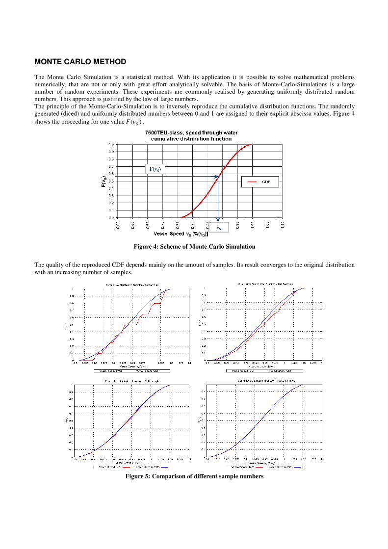
MONTE CARLO METHOD The Monte Carlo Simulation is a statistical method. With its application it is possible to solve mathematical problems numerically, that are not or only with great effort analytically solvable. The basis of Monte-Carlo-Simulations is a large number of random experiments. These experiments are commonly realised by generating uniformly distributed random numbers. This approach is justified by the law of large numbers. The principle of the Monte-Carlo-Simulation is to inversely reproduce the cumulative distribution functions. The randomly generated (diced) and uniformly distributed numbers between 0 and 1 are assigned to their explicit abscissa values. Figure 4 shows the proceeding for one value )( SvF .

Figure 4: Scheme of Monte Carlo Simulation

The quality of the reproduced CDF depends mainly on the amount of samples. Its result converges to the original distribution with an increasing number of samples.

Figure 5: Comparison of different sample numbers

OVERVIEW OF ALGORITHM Figure 6 gives an overview of the program cycle (MonteProp algorithm):

Starting with an existing ship design, the best matching Noon-to-Noon and environmental data have to be selected. Applying the Monte Carlo Method, the necessary vessel specific and environmental parameters are determined. For each of these operating points the equilibrium condition is simulated. Already implemented manoeuvring algorithms incorporate the vessel’s propulsion. Additional resistances due to environmental conditions are considered, applying empiric and direct calculation methods.

Stillwater Resistance: The vessel’s actual resistance is computed basing on previously generated resistance curves. Either they are available through model tests or they have been computed, using common methods (e.g. via a suitable vessel of comparison or standard series). According to ITTC 57 the total resistance is:

RFT RRR +=

The frictional resistance RF depends on the vessel’s speed and its actual wetted surface. It is calculated directly. The residual resistance mainly represents the wave making resistance. Its coefficient cR is only available for the given resistance curves, which are commonly recorded for conditions on even keel when performing model tests. The influence of trim on the wave making resistance is taken into account as described and validated by Eljardt (2006) for container vessels. For the MonteProp algorithm, Eljardt’s proceeding of splitting and recombining cR has been modified in order to cover different vessel types and a wider trim range.

Existing Ship Design Floating Condition, Environment, Propulsion Plant from Logbook

(Noon-to-Noon Data)

Voyage Profile as Stochastic Distribution (through Monte-Carlo-Simulations)

Computation of Equilibrium Condition for Given Operating Point, Using Manoeuvring

Algorithms (Drift- and Rudder Angle), including aligned Environmental Conditions

Computation of Added Resistances and Required Power Output

Interface for Various Applications

Evaluation and Optimisation of Given and Revised Designs

Prediction of Risk for Rudder Cavitation

…

Detailed numerical model, including hydrostatics, resistance and propulsion

Figure 6: Flowchart of MonteProp-algorithm

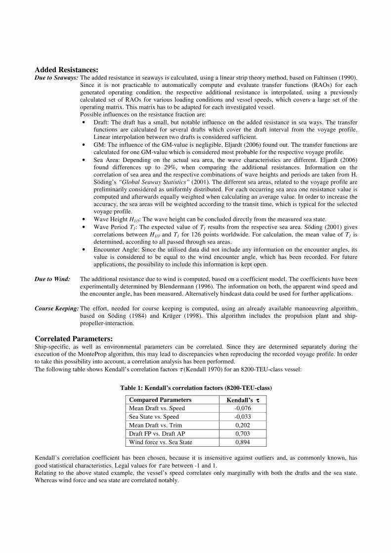
Added Resistances: Due to Seaways: The added resistance in seaways is calculated, using a linear strip theory method, based on Faltinsen (1990).

Since it is not practicable to automatically compute and evaluate transfer functions (RAOs) for each generated operating condition, the respective additional resistance is interpolated, using a previously calculated set of RAOs for various loading conditions and vessel speeds, which covers a large set of the operating matrix. This matrix has to be adapted for each investigated vessel.

Possible influences on the resistance fraction are: • Draft: The draft has a small, but notable influence on the added resistance in sea ways. The transfer

functions are calculated for several drafts which cover the draft interval from the voyage profile. Linear interpolation between two drafts is considered sufficient.

• GM: The influence of the GM-value is negligible, Eljardt (2006) found out. The transfer functions are calculated for one GM-value which is considered most probable for the respective voyage profile.

• Sea Area: Depending on the actual sea area, the wave characteristics are different. Eljardt (2006) found differences up to 29%, when comparing the additional resistances. Information on the correlation of sea area and the respective combinations of wave heights and periods are taken from H. Söding’s “Global Seaway Statistics” (2001). The different sea areas, related to the voyage profile are preliminarily considered as uniformly distributed. For each occurring sea area one resistance value is computed and afterwards equally weighted when calculating an average value. In order to increase the accuracy, the sea areas will be weighted according to the transit time, which is typical for the selected voyage profile.

• Wave Height H1/3: The wave height can be concluded directly from the measured sea state. • Wave Period T1: The expected value of T1 results from the respective sea area. Söding (2001) gives

correlations between H1/3 and T1 for 126 points worldwide. For calculation, the mean value of T1 is determined, according to all passed through sea areas.

• Encounter Angle: Since the utilised data did not include any information on the encounter angles, its value is considered to be equal to the wind encounter angle, which has been recorded. For future applications, the possibility to include this information is kept open.

Due to Wind: The additional resistance due to wind is computed, based on a coefficient model. The coefficients have been

experimentally determined by Blendermann (1996). The information on both, the apparent wind speed and the encounter angle, has been measured. Alternatively hindcast data could be used for further applications.

Course Keeping: The effort, needed for course keeping is computed, using an already available manoeuvring algorithm,

based on Söding (1984) and Krüger (1998). This algorithm includes the propulsion plant and ship-propeller-interaction.

Correlated Parameters: Ship-specific, as well as environmental parameters can be correlated. Since they are determined separately during the execution of the MonteProp algorithm, this may lead to discrepancies when reproducing the recorded voyage profile. In order to take this possibility into account, a correlation analysis has been performed. The following table shows Kendall’s correlation factors τ (Kendall 1970) for an 8200-TEU-class vessel:

Table 1: Kendall’s correlation factors (8200-TEU-class)

Compared Parameters Kendall’s ττττ

Mean Draft vs. Speed -0,076

Sea State vs. Speed -0,033

Mean Draft vs. Trim 0,202

Draft FP vs. Draft AP 0,703

Wind force vs. Sea State 0,894 Kendall’s correlation coefficient has been chosen, because it is insensitive against outliers and, as commonly known, has good statistical characteristics. Legal values for τ are between -1 and 1. Relating to the above stated example, the vessel’s speed correlates only marginally with both the drafts and the sea state. Whereas wind force and sea state are correlated notably.

Wind Force vs. Sea State: When comparing the cumulative distribution functions of parameters, great resemblance in shape can be observed. Figure 6

shows both CDFs after the wind force CDF has been reduced by a constant factor of 1BF.

Figure 6: Reduced Wind Force vs. Recorded Sea State

TFP vs. TAP / TAVG vs. Trim In order to determine the most practicable method to reproduce the draft and trim CDFs correctly, different dicing sequences have been implemented and compared with the original distributions.

a) Subsequent dicing of the drafts, afterwards check, whether trim is in measured trim range. If not, the second draft is diced again.

b) Subsequent dicing of one draft (TAP) and a trim, afterwards it is checked, whether TFP is in given draft range. If not, the trim will be diced again.

Both proceedings result in slightly deviating CDFs for the subsequently diced parameters. Therefore it was decided to modify the dicing sequence in order to increase the accuracy:

c) After TAP is diced, a trim distribution is chosen depending on its value. From this CDF, a trim value is derived. Like in b) it is subsequently checked, whether TFP is in its given range, if not a new trim value is diced. In the case of the 8200-TEU-class vessel, 6 different draft intervals have been picked and the respective trim distribution functions have been determined. The two representative CDFs shown in Figure 7 point out how different the trim distribution can be, depending on the draft interval ∆T (∆T2 < ∆T4):

Figure 7: Different Trim CDFs, depending on TAP interval (8200-TEU-class)

Utilizing the above-described procedure, the correlation of the second draft is acknowledged more precisely when

following c), but the trim CDF is reproduced worse than acc. to b), see Figure 8 below:

b) c)

Figure 8: Comparison of Draft and Trim CDFs, diced acc. to b) and c)

Since TAP is diced first, both CDFs are reproduced equally congruent.

In conclusion, it was decided to remain with only one trim CDF and dicing sequence b). The correlation between the two drafts (and therefore the influence of the trim distribution) is higher than between averaged draft and trim. Sequence b) also saves calculating time, since fewer combinations have to be eliminated because of illegal draft combinations. Nevertheless, this problem has to be considered again, when implementing the dicing sequence for other vessel types and/or voyage profiles.

VALIDATION OF ALGORITHM The implemented MonteProp-algorithm has been validated, using recorded measurements of the main engine’s power output. This parameter was recorded with the help of a shaft power measuring system and can be used directly for the comparison. Eljardt (2006) investigated the accuracy of this method and proved it to be sufficient. If all subsequently executed methods provide reliable results the simulated shaft power distribution should be mostly congruent with the recorded one. Herewith the correctness of the algorithm would be proved.

Figure 9: Comparison of Simulated and Measured Shaft Power CDF

The diagram, shown in Figure 9, compares the simulated and the measured shaft power CDFs of the 8200-TEU-class vessel. The function’s congruence is satisfactory, when considering the applied input data, its simplifications and the utilized methods with its incorporated numeric models. Since not all characteristics of the original CDF are congruent, there is still room for improvement and adaption of the various method interfaces. In the time until IMDC 2009, the validation process will be extended, using measurements of a fast single-screw RoRo-Ferry and other Container Vessels.

RESULTS A first benchmarking analysis has been performed, using the 8200-TEU-class vessel as a reference.

Figure 10: Frame Plan of Reference Vessel 8200-TEU-Class

The most important main particulars are:

Table 2: Main Particulars 8200TEU Reference Vessel

Length over all, LOA 334.00m Breadth, B 42.80m Draft Design, TD 13.00m Design Speed, vD 25.3kn DWT 100,800mt

The following figure shows the probability density functions of the required main engine power output, resulting from different resistance curve sets. The blue probability distribution represents the initial design, the green PDF is simulated, using reduced resistance curves for design and intermediate draft, accepting an increased resistance on full scantling draft:

Figure 11: Shaft Power PDF for Different Resistance Curve Sets

The changed resistance curve compilation results in a shifted centre of gravity (COG), which is marked by a vertical bar. If its value declines, this means, during the lifetime, the averaged engine power demand and as a direct result the overall fuel consumption decreases. Figure 12 shows both resistance curve sets. The first set contains the four model test curves. The second set consists of the original ballast curve, the reduced curves for intermediate and design draft curves and concluding the increased resistance curve on full scantling draft. This compilation is intended to reproduce a realistic optimisation result. An improvement on a certain draft interval incorporates a worsening for other drafts. Lange (2005) showed that notable resistance reductions are achievable, even with contemporary container ship designs. The results were proved with CFD calculations, using the potential flow code KELVIN, developed by Söding (1999). Potential flow codes are less suitable to predict absolute resistance values, but they showed to be fairly reliable when predicting the effect of design changes in relation to the initial design.

Figure 12: Resistance Curves – Model Test Results & Optimized Set

On the basis of Lange’s Diploma Thesis (2005) a hullform optimisation will be executed until IMDC 2009.

BENCHMARKING OF RUDDER DESIGNS REGARDING THE CAVITATION RISK Based on the results of the above explained Monte-Carlo driven manoeuvring simulation an evaluation of different aspects of the ship design is possible. A useful application of this approach is the benchmarking of different rudder designs regarding the cavitation risk within the operational profile. Usually a rudder design for example is, if any, only tested against rudder cavitation for a few rudder angles under design conditions. To get an idea of the expectant cavitation risk level of the rudder design, the above mentioned method is able to provide the expectant operation conditions. Afterwards the determination of the cavitation risk itself is based on this operational profile. Figure 13 shows exemplary the operational profile of a roll-on roll-off ferry with a design speed vD of 23 knots. The data is taken from measurements during 11 months of operation (Greitsch 2008).

Figure 13 - Frequency Distribution of Rudder Angles and Ship Speeds

Considering the frequency distributions of rudder angles and vessel speeds it is noticeable that the rudder angles are Gaussian distributed as expected. On the other hand the vessel sails most of the time with average speed values about 5 knots below design speed. In addition, there is a small accumulation of occurred vessel speeds in the range of 7.5 knots, which indicates slow speed manoeuvring. Figure 14 shows the cumulative density function of the operational profile of the ferry (black lines) and the above mentioned 8200TEU container vessel (red lines). Comparing the operational profiles of the two vessels, it is obvious that especially the speed profiles of the vessels differ in terms of the slow speed rate due to a high rate of estuary trading in the case of the ferry.

Figure 14 – Comparison of the Operational Profiles

The parameters of the operational profile can be considered independent because there is no significant correlation between the ship speeds and the rudder angles in the investigated cases. The calculated correlation factors are shown in Table 3.

Table 3 – Calculated Correlation Factors

8200TEU container vessel Roll-on roll-off ferry Correlation factor τ (Kendall) -0.22 -0.11

The cavitation prognosis is carried out with a panel code based on the potential flow theory (Söding 1998) and (Krüger 1998). This allows very fast calculations and therefore the analysis of a large number of observed operation cases in a finite time period. The used CFD code takes into account the wake field of the observed vessel and the propeller slipstream calculated with the lifting line method. The downstream velocities are calculated by the use of the Lerbs’ induction factors. As a conservative criterion the cavitation is calculated by comparing the local pressure with the vapour pressure of the passing water at the observed location (Krüger 2002). The interpretation of the results is carried out by a cavitation coefficient ccav as a saltus function which has the value 0 for non-cavitating situations of this panel and the value 1 in case of cavitation on the observed panel. In order to benchmark the cavitation risk for different regions on the rudder the cavitation occurrence on each panel is weighted by the frequency of the operation situation. Therefor the operational profile is classified into m classes of rudder angles δ and n classes of combinations of vessel speeds vs und propeller thrusts T. The thrust demand for the different operating situations includes the additional demand regarding the environmental influences like wind and sea state. The calculation of all combinations of rudder angles and fixed pairs of vessel speeds and propeller thrusts leads to a safety against cavitation Scav for each panel:

)),()((1 ,

1,,

1jjsi

n

j

jicav

m

i

cav TvffcS ⋅⋅−= ∑∑==

δ [1]

A value of Scav=1 specifies a 100 percent safety against cavitation for the observed panel in the range of operation situations. Resulting from the saltus function there can be no safety greater than 1. In the same manner a value of Scav=0 indicates, that the observed panel would cavitate in all operation situations. To demonstrate the ability of the method to benchmark different rudder design with the safety index, the cavitation safety distribution of two different rudder designs are calculated for the determined operational profile. The visualization of the calculated safety against cavitation is shown in Figure 15 and Figure 16. Both rudder versions are carried out as symmetric rudders with a tapered leading edge.

Figure 15 – Cavitation Safety Distribution – Design A

The two different rudder designs differ only in the used profile type. Design A is based on NACA 4-digit profiles and is representative for a rather poor design. Design B is modeled with profiles from the NACA-64 series. It is obvious, that both design stages only show a cavitation risk at the upper leading edge due to the rotation effect imposed by the right turning propeller. In this case the influence of the different profile shapes does not affect the minimum safety level of about 60% safety against cavitation within the whole operational profile, but the size of the area, which shows this reduced safety level. By contrast a rudder shape modification in terms of asymmetric profile shapes, like twisted leading edges, leads to an increased safety level, whereas the area of possible cavitation stays nearly constant. Comparative calculations of different twisted rudders using the example of the roll-on roll-off ferry were presented by Greitsch (2008).

Figure 16 - Cavitation Safety Distribution – Design B

DNV – CLASS AND BEYOND The design approach described in the paper has various involvement connected with the life cycle of a vessel. Some involvement is connected with the traditional work of a classification society, some belongs to the beyond class DNV capabilities. The possibilities of predicting the risk of cavitation on the rudder may imply different rudder strength requirements. Different cargo and ballast distribution or evolved weather routing tools would influence the fatigue life of the vessel as well as the possibility of having different slamming probability. Moreover DNV has tools allowing computational analyses to estimate the vessel loads as well as the hull resistance permitting an early evaluation of the economical impact of any design modification. These tools can help to verify the evaluations of the work carried out by the authors.

CONCLUSIONS This paper showed a new approach to benchmark different ship designs, keeping a clear focus on the operation. It has been proved that it is possible to simulate a complete lifecycle of a projected vessel, using fore- and hindcasted operation data (ship-specific and environmental). The simulation results, regarding the power demand, are available in rather short computation time. The use of an entire manoeuvring simulation leads to a complete database of operational data. On the basis of this simulation it is possible to implement various successive methods in order to evaluate and optimise the design regarding operational efficiency and also ship safety. In addition it is now possible to reliably number the achievable savings or contrary the additional expenditures of an inferior design on a lifetime basis. The determination of the rudder cavitation risk, as shown, allows the comparison of different rudder designs within the expected operational profile of the vessel.

REFERENCES BERTRAM, V., “Practical Ship Hydrodynamics”, Oxford: Butterworth-Heinemann, 2002

BLENDERMANN, W., “Wind Loading of Ships – Collected Data from Wind Tunnel Tests in Uniform Flow”, Inst. f. Schiffbau der Universität Hamburg – Bericht Nr. 574, 1996

BRIX, J. E., “Manoeuvring Technical Manual”, Hamburg: Seehafen Verlag, 1993

ELJARDT, G., “Development of a Fuel Oil Consumption Monitoring System”, Diploma Thesis TUHH, Hamburg, 2006 (to be obtained from the author)

FALTINSEN, O. M. “Sea Loads on Ships and Offshore Structures”, Cambridge; New York: Cambridge University Press, 1990

GREITSCH, L., “Prognosis of Rudder Cavitation Risk in Ship Operation”, Numerical Towing Tank Symposium, Brest, 2008

KENDALL, M.G., “Rank Correlation Methods”, London: Griffin, 1970

KRÜGER, S., “A Panel Method for Predicting Ship-Propeller Interaction in Potential Flow”, Ship Technology Research Vol. 45, Hamburg, 1998

KRÜGER, S., “Manövriersimulation auf der Basis von Großausführungsmessungen”, JSTG Vol. 92, Berlin: Springer Verlag, 1998

KRÜGER, S., “Kavitation an Halbschweberudern schneller Fähren”, TU Hamburg Harburg – Technical Report, 2002

LANGE, N., “Widerstandsoptimierung eines PanMax-Containerschiffes”, Diploma Thesis TUHH, Hamburg, 2005 (to be obtained from the author)

SCHLICHTING, O., “Schiffswiderstand auf beschränkter Wassertiefe”, JSTG Vol. 35, Berlin: Strauß, Vetter & Co., 1934

SOBOL, I. M., “The Monte Carlo Method”, Moscow: Mir Publishers, 1984

SÖDING, H., “Bewertung der Manövriereigenschaften im Entwurfsstadium”, JSTG Vol. 78, Berlin: Springer Verlag, 1984

SÖDING, H., “Limits of Potential Theory in Rudder Flow Predictions”, Ship Technology Research Vol. 45, Hamburg, 1998

SÖDING, H., “Das Wellenwiderstands-Programm Kelvin”, Inst. f. Schiffbau der Universität Hamburg, 1999

SÖDING, H., “Global Seaway Statistics”, Inst. f. Schiffbau der Universität Hamburg – Bericht Nr. 610, 2001