openEMS a free and open source equivalentcircuit (EC) … · this unwanted numerical slow-down. The performance of the cylindrical EC FDTD implementation is presented in Section 5

INTERNATIONAL JOURNAL OF NUMERICAL MODELLING: ELECTRONIC NETWORKS, DEVICES AND FIELDSInt. J. Numer. Model. 2012Published online in Wiley Online Library (wileyonlinelibrary.com). DOI: 10.1002/jnm.1875

openEMS – a free and open source equivalent-circuit (EC) FDTDsimulation platform supporting cylindrical coordinates suitable for

the analysis of traveling wave MRI applications

Thorsten Liebig!;!, Andreas Rennings, Sebastian Held and Daniel Erni

General and Theoretical Electrical Engineering (ATE), Faculty of Engineering, University of Duisburg-Essen, andCENIDE - Center for Nanointegration Duisburg-Essen, D-47057 Duisburg, Germany

SUMMARY

In this paper, we present a free and open source platform by using the equivalent-circuit finite-difference time-domain (FDTD) method adapted to cylindrical coordinates to efficiently model cylindrically shaped objects. Wewill address the special characteristics of a cylindrical FDTD mesh such as the mesh singularity at r D 0 anddiscuss how cylindrical subgrids for small radii can reduce the simulation time considerably. Furthermore, wewill demonstrate the applicability and advantages of this cylindrical equivalent-circuit FDTD method to evaluatenew types of conformal ring antennas used in the context of high-field (7T) traveling wave magnetic resonanceimaging (MRI). Copyright © 2012 John Wiley & Sons, Ltd.

Received 2 March 2012; Revised 10 July 2012; Accepted 3 October 2012

KEY WORDS: FDTD; EC FDTD; cylindrical mesh; multigrid; traveling wave MRI

1. INTRODUCTION

The finite-difference time-domain (FDTD) method is one of the most successful explicit and directnumerical methods to solve large and complex electromagnetic field problems [1,2]. Its greatest benefitis the simple and straightforward approach allowing a memory and computationally efficient imple-mentation. The conventional field-based version of the FDTD method [1, 2] relies on both the electricand magnetic field components involving the typical leapfrogged multiply-and-add updating schemefor the well-known time evolution. An alternative approach is the use of state variables such as voltagesand currents instead of field quantities where the FDTD algorithm is then operating in the framework ofa corresponding passive equivalent circuit (EC). Such an EC representation is attractive because it bearsa very intuitive access to the implementation of material dispersion. The first mention of EC FDTDappears, to our knowledge, in the publications of Gwarek et al. [3] and Craddock et al. [4]. Initialimplementations of the proposed EC FDTD algorithm have been carried out for a regular Cartesianmesh, as it has been initially described in [5, 6] and more extensively in [7, 8]. Following Maxwell’sequations, the proper EC formulation is directly deducible from its differential form (which is certainlyconstitutive for the conventional FDTD scheme) or from its integral form, where the latter defines thevery starting point of our EC FDTD scheme as well as for other methods such as the well-establishedfinite-integral technique (FIT) [9, 10]. In either case, the EC FDTD algorithm can easily be translatedback and forth to the conventional FDTD formulation and therefore retains most of its advantages anddisadvantages, concerning, for example, numerical accuracy and stability.

!Correspondence to: Thorsten Liebig, General and Theoretical Electrical Engineering (ATE), Faculty of Engineering, Universityof Duisburg-Essen, and CENIDE - Center for Nanointegration Duisburg-Essen, Bismarckstr. 81, D-47057 Duisburg, Germany.!E-mail: [email protected]

Copyright © 2012 John Wiley & Sons, Ltd

( )

2 T. LIEBIG ET AL.

It is worth noting that the EC FDTD formulation has clear benefits such as a reduced numericaleffort inside the iteration loop because of a reduced number of multiplications (which is intrinsic tothe representation with state variables such as voltages and currents) and the aforementioned intuitiveincorporation of (highly) dispersive materials. For example, materials that are represented by multi-polar Drude/Lorentz type models [7, 8] can be easily implemented along corresponding extensions ofthe associated EC in the form of small tailored filter sections, which mimics the material dispersionunderlying, for example, plasmonic structures [11, 12], wide band-conducting sheet models [6], oreven more challenging material properties such as biological tissue [13]. An additional virtue of the ECFDTD formulation is its affinity to an energy-based stability criterion [7, 8] that tends to be less strictthan the usually applied Courant–Friedrich–Levy (CFL) stability criterion. Interestingly, this alterna-tive criterion is in principle also applicable to the conventional FDTD scheme offering thus a promisefor potentially larger time steps.

In the following, we will show that an adaption of our EC FDTD algorithm to a cylindricalmesh can be realized with only minimal changes to the EC FDTD operator coefficients allow-ing the use of a generic (and potentially highly optimized) EC FDTD iteration engine whileenabling all well-known FDTD features (e.g., perfectly matched layer (PML) boundary conditions,Mur-absorbing boundary conditions, dispersive material models, and conducting sheet models) atvirtually unaltered numerical efficiency. Please note that our cylindrical EC FDTD implementa-tion is more general than the body of revolution version of FDTD provided, for example, by otherFDTD simulation packages such as MEEP [14] because the body of revolution representation isrestricted to rotationally symmetric problems, whereas our proposed method qualifies as a full vec-torial three-dimensional (3D) EC FDTD scheme adapted to cylindrical r-coordinates, ˛-coordinates,and ´-coordinates.

Cylindrical FDTD implementations—and in particular for magnetic resonance imaging (MRI)applications—have already been carried out, for example, by Trakic et al. [15] for the analysisof transient eddy currents stemming from switching magnetic field gradients as well as byChi et al. [16] for the comprehensive analysis of radio-frequency (RF) field-tissue interactions. Inaddition, Wang et al. [17] proposed a parallelization scheme for an earlier FDTD version support-ing both Cartesian and cylindrical meshes, which relies on a distributed memory architecture whileadapting the message-passing interface (MPI) library. Chi et al. [16] was also offering a numerical reg-ularization scheme for handling the polar-axis singularity apparent in the cylindrical implementation,using Ampère’s and Faraday’s laws as an indirect access to the field quantities in the singularity. Alter-native measures based on corresponding coordinate transformations are proposed by Kancleris [18].The authors [16] also speculates about the need for subgridding that may possibly become an issueto be considered because of the costly mesh refinement inherent to the morphology of the cylindricaldiscretization. In our paper, we will demonstrate that subgridding is less an option than an inevitablefeature to be included in any cylindrical FDTD implementation because of the severe constraints posedby the CFL limit (or a similar energy-based criterion [7, 8]).

The remainder of the paper is organized as follows: after an introduction into the EC FDTD formu-lation for the Cartesian grid in Section 2, we will reiterate the EC FDTD formulation for the cylindricalYee cell in Section 3 while investigating two emerging special cases of the staggered grid that onlyoccur in a cylindrical mesh and, hence, how to handle these cases effectively. This also includes theregularization of the polar-axis singularity in the EC formulation following a similar approach as in[16]. In Section 4, we will address the issue of the reduced FDTD time step due to the mesh refinementpresent in any regular cylindrical grid and introduce an efficient subgridding strategy to counteractthis unwanted numerical slow-down. The performance of the cylindrical EC FDTD implementationis presented in Section 5 along two examples, namely a simple benchmark problem and a showcasefrom our ongoing MRI research. In the framework of novel scanner schemes such as the high-fieldtraveling wave (TW) MRI [19], where the RF magnetic field exposure is provided by propagating elec-tromagnetic modes along the cylindrical MRI bore, we have analyzed thin ring antennas, on the basisof composite right/left-handed (CRLH) electromagnetic metamaterials [20] for molding the resultingwave fields [21, 22]. As these excitation antennas are conforming to the inner surface of the MRIbore, the resulting simulation problem becomes highly challenging because of the thin sophisticatedfeatures that are embedded in the large bore volume. We can show that the cylindrical EC FDTD

Copyright © 2012 John Wiley & Sons, LtdDOI: 10.1002/jnm

Int. J. Numer. Model. (2012)

openEMS—A FREE AND OPEN SOURCE EC FDTD SIMULATION PLATFORM 3

implementation turns out to be ideally suited to demonstrate the applicability of the metamaterial ringantennas as a holistic excitation and control scheme in traveling wave MRI.

Practical information regarding the proper implementation of the free and open source EC FDTDsimulation platform openEMS [23] is provided in Section 6. This includes software issues as well asperformance measures together with a short description of the user-friendly Matlab/Octave scriptinginterface. The interface is designed to setup, control, and evaluate the EC FDTD simulation and alsoacts as a simple graphical user interface (GUI) in the sense of a two-dimensional (2D)/3D structuralviewer. Hence, openEMS is made available for public review, free use, and participative enhancement.A brief conclusion together with an outlook is finally drawn in Section 7.

2. THE EC FDTD FORMULATION IN CARTESIAN COORDINATES

The EC FDTD scheme in Cartesian coordinates is derived from Maxwell’s equations in integral form,

I@ QA

EH ! dEs D C ddt

“QA" EE ! d EQA C

“QA! EE ! d EQA (1)

I@A

EE ! dEs D " ddt

“A

" EH ! d EA "“

A

# EH ! d EA (2)

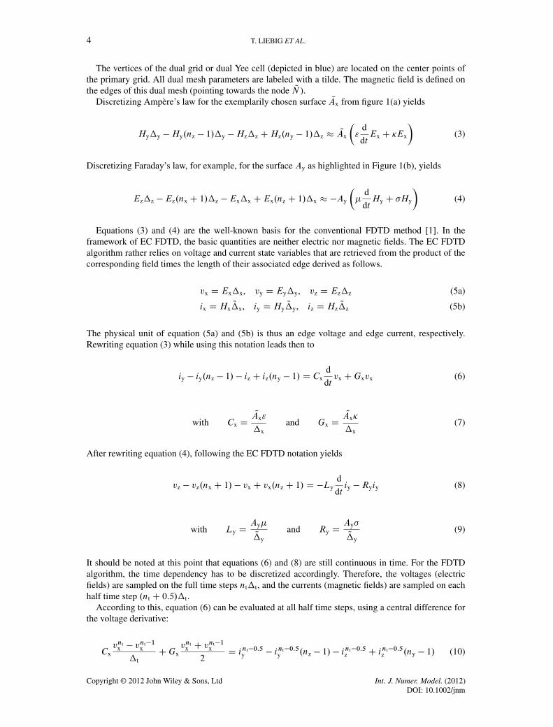
where all material properties, (permitivity ", permeability ", electric conductivity !, and mag-netic conductivity #) are for clarity reasons considered nondispersive (i.e., frequency independent).These time-continuous and space-continuous equations have to be discretized using the well-knownYee cell [1] depicted in Figure 1.

The so-called primary grid (shown in red) is introduced by the user (or software) according to thegiven simulation structure. The electric field is defined on the edges originating on the primary node(N in Figure 1) of the primary grid, where the length of an edge, for example, in the x-direction,is labeled as $x. It should be noted that the proposed scheme fully supports a graded mesh in anydirection, which makes the length of the edges depend on the position inside the mesh. For a betterreadability, a notation such as $x.nx/ was omitted.

The faces of the primary Yee cell, for example, normal to the y-axis, are labeled Ay (cf. Figure 1(b)).

(a) (b)

Figure 1. Yee cell (a) highlighting Ampère’s law for the electric field in x-direction through surface QAx and inassociation with the surrounding magnetic field components in y-direction and ´-direction and (b) highlightingFaraday’s law for the magnetic field in y-direction through surface Ay and in association to the surrounding

electric field components in x-direction and ´-direction.



4 T. LIEBIG ET AL.

The vertices of the dual grid or dual Yee cell (depicted in blue) are located on the center points ofthe primary grid. All dual mesh parameters are labeled with a tilde. The magnetic field is defined onthe edges of this dual mesh (pointing towards the node QN ).

Discretizing Ampère’s law for the exemplarily chosen surface QAx from figure 1(a) yields

Hy$y " Hy.nz " 1/$y " Hz$z C Hz.ny " 1/$z # QAx

!"

ddt

Ex C !Ex

"(3)

Discretizing Faraday’s law, for example, for the surface Ay as highlighted in Figure 1(b), yields

Ez$z " Ez.nx C 1/$z " Ex$x C Ex.nz C 1/$x # "Ay

!"

ddt

Hy C #Hy

"(4)

Equations (3) and (4) are the well-known basis for the conventional FDTD method [1]. In theframework of EC FDTD, the basic quantities are neither electric nor magnetic fields. The EC FDTDalgorithm rather relies on voltage and current state variables that are retrieved from the product of thecorresponding field times the length of their associated edge derived as follows.

vx D Ex$x, vy D Ey$y, vz D Ez$z (5a)

ix D Hx Q$x, iy D Hy Q$y, iz D Hz Q$z (5b)

The physical unit of equation (5a) and (5b) is thus an edge voltage and edge current, respectively.Rewriting equation (3) while using this notation leads then to

iy " iy.nz " 1/ " iz C iz.ny " 1/ D Cxddt

vx C Gxvx (6)

with Cx DQAx"

$xand Gx D

QAx!

$x(7)

After rewriting equation (4), following the EC FDTD notation yields

vz " vz.nx C 1/ " vx C vx.nz C 1/ D "Lyddt

iy " Ryiy (8)

with Ly D Ay"

Q$yand Ry D Ay#

Q$y(9)

It should be noted at this point that equations (6) and (8) are still continuous in time. For the FDTDalgorithm, the time dependency has to be discretized accordingly. Therefore, the voltages (electricfields) are sampled on the full time steps nt$t, and the currents (magnetic fields) are sampled on eachhalf time step .nt C 0:5/$t.

According to this, equation (6) can be evaluated at all half time steps, using a central difference forthe voltage derivative:

Cxvnt

x " vnt"1x

$tC Gx

vntx C vnt"1

x

2D int"0:5

y " int"0:5y .nz " 1/ " int"0:5

z C int"0:5z .ny " 1/ (10)




Assuming that the voltages and currents prior to the current time step nt are known, this yields the firstupdate equation for, for example, the voltage vx:

vntx D 2Cx " $tGx

2Cx C $tGxvnt"1

x C 2$t

2Cx C $tGx

#int"0:5y " int"0:5

y .nz " 1/ " int"0:5z C int"0:5

z .ny " 1/$

(11)

In practice this means that no additional data have to be stored, and equation (11) will access the latestvalue of vx that is of time step nt " 1 and overwrite it to be the current voltage at time step nt.

When the discretized time scheme is applied to equation (8), one obtains the expression:

LyintC0:5y " int"0:5

y

$tC Ry

intC0:5y C int"0:5

y

2D vnt

z " vntz .nx C 1/ " vnt

x C vntx .nz C 1/ (12)

Again, given the voltages and currents prior to the time step nt C 0:5, equation (12) yields the secondupdate equation for, for example, the current iy:

intC0:5y D 2Ly " $tRy

2Ly C $tRyint"0:5y " 2$t

2Lx C $tRy

%vnt

z " vntz .nx C 1/ " vnt

x C vntx .nz C 1/

&(13)

The EC FDTD algorithm iteratively updates both sets of equations (11) and (13) until a particulartermination criterion is met such as a complete dissipation of energy from the simulation domain or asteady state is reached in case of a sinusoidal excitation.

As mentioned in the introduction, the major advantage of the EC FDTD over the conventional FDTDmethod is its higher computational efficiency that can be recognized, for example, in voltage updateequation (11). The EC FDTD needs only two coefficients and two multiplications for each update,compared with the three coefficients and multiplications for the conventional FDTD scheme. Thisoverall reduction pays off with respect to a considerable speed and memory improvement of 33%.

It is worth mentioning that the EC FDTD bears some similarities to the so-called FIT [9], whichcan be viewed as a powerful extension of the FDTD scheme towards unstructured meshes. In FIT, fouradditional state variables are operational from the corresponding integral relations involving electricand magnetic flux densities as well as the current and charge densities. Referring to the smaller numberof state variables, EC FDTD is believed to be numerically less expensive. It is although still supportinga high level of accuracy (compared with conventional FDTD) owing to the well-adapted sampling andaveraging of material boundaries in the Yee cell that comes along with the EC form associated to thecorresponding state variable.

3. THE EC FDTD FORMULATION IN CYLINDRICAL COORDINATES

The EC FDTD formulation for cylindrical coordinates is mostly identical to the Cartesian implemen-tation as derived in Section 2. Figure 2 illustrates the Yee cell for the particular geometries. As for theCartesian grid, Maxwell’s equations (1) and (2) are evaluated on the surfaces and edges of the cylindri-cal Yee cell. The derivation of the final update/iteration equations is identical to the Cartesian case. Theupdate equations for the two exemplary chosen voltage respective current state variable (cf. Figure 2)are therefore written as

vntr D 2Cr " $tGr

2Cr C $tGrvnt"1

r C 2$t

2Cr$tGr

%int"0:5˛ " int"0:5

˛ .nz " 1/ " int"0:5z C int"0:5

z .n˛ " 1/&

(14)



6 T. LIEBIG ET AL.

(a) (b)

Figure 2. Yee cell (a) highlighting Ampère’s law for the electric field in r-direction through surface QAr andin association to the surrounding magnetic field components in ˛-direction and ´-direction and (b) highlightingFaraday’s law for the magnetic field in ˛-direction through surface A˛ and in association to the surrounding

electric field components in r-direction and ´-direction.

with Cr DQAr"

$rand Gr D

QAr!

$r(15)

intC0:5˛ D 2L˛ " $tR˛

2L˛ C $tR˛int"0:5˛ " 2$t

2Lr C $tR˛

%vnt

z " vntz .nr C 1/ " vnt

r C vntr .nz C 1/

&(16)

with L˛ D A˛"

Q$˛ Qrand R˛ D A˛#

Q$˛ Qr(17)

Comparing the EC FDTD update equations for the Cartesian mesh in equations (11) and (13) tothe cylindrical mesh update equations (14) and (16) reveals the identical formulation for the updatecoefficients. The only difference between the Cartesian and cylindrical formulation emerges in thecalculation of the surface areas Ad , QAd (with d 2 r; ˛; z) and edge lengths $d , Q$d needed to evaluatethe EC FDTD quantities Cd , Gd , Ld , and Rd . As well as for the Cartesian mesh, this formulationallows for an arbitrary mesh grading in r-direction, ˛-direction, or ´-direction, if the appropriate meshposition is considered to calculate this quantities. Furthermore, it is important to note that the edgelengths in ˛-direction are a product of the respective angular widths $˛ , Q$˛ and the edge radii r , Qr(cf. equation (17)).

The mesh shown in Figure 3(a) is an example for a typical cylindrical mesh, but as distinguishedfrom the Cartesian mesh, the cylindrical mesh encompasses two special cases that have to be handled

(a) (b)

Figure 3. Yee cells of the staggered grid in a cylindrical coordinate system with (a) an “open” and with (b) a“closed” ˛-mesh.




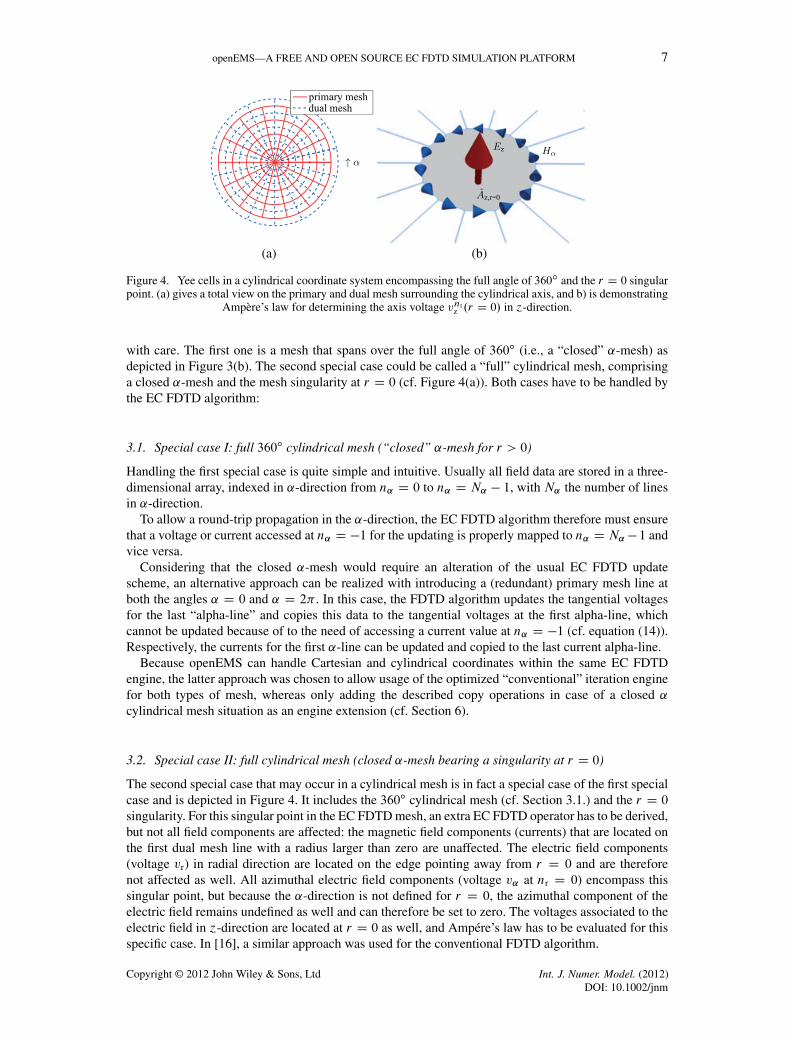
(a) (b)

Figure 4. Yee cells in a cylindrical coordinate system encompassing the full angle of 360ı and the r D 0 singularpoint. (a) gives a total view on the primary and dual mesh surrounding the cylindrical axis, and b) is demonstrating

Ampère’s law for determining the axis voltage vntz .r D 0/ in ´-direction.

with care. The first one is a mesh that spans over the full angle of 360ı (i.e., a “closed” ˛-mesh) asdepicted in Figure 3(b). The second special case could be called a “full” cylindrical mesh, comprisinga closed ˛-mesh and the mesh singularity at r D 0 (cf. Figure 4(a)). Both cases have to be handled bythe EC FDTD algorithm:

3.1. Special case I: full 360ı cylindrical mesh (“closed” ˛-mesh for r > 0)

Handling the first special case is quite simple and intuitive. Usually all field data are stored in a three-dimensional array, indexed in ˛-direction from n˛ D 0 to n˛ D N˛ " 1, with N˛ the number of linesin ˛-direction.

To allow a round-trip propagation in the ˛-direction, the EC FDTD algorithm therefore must ensurethat a voltage or current accessed at n˛ D "1 for the updating is properly mapped to n˛ D N˛ " 1 andvice versa.

Considering that the closed ˛-mesh would require an alteration of the usual EC FDTD updatescheme, an alternative approach can be realized with introducing a (redundant) primary mesh line atboth the angles ˛ D 0 and ˛ D 2% . In this case, the FDTD algorithm updates the tangential voltagesfor the last “alpha-line” and copies this data to the tangential voltages at the first alpha-line, whichcannot be updated because of to the need of accessing a current value at n˛ D "1 (cf. equation (14)).Respectively, the currents for the first ˛-line can be updated and copied to the last current alpha-line.

Because openEMS can handle Cartesian and cylindrical coordinates within the same EC FDTDengine, the latter approach was chosen to allow usage of the optimized “conventional” iteration enginefor both types of mesh, whereas only adding the described copy operations in case of a closed ˛cylindrical mesh situation as an engine extension (cf. Section 6).

3.2. Special case II: full cylindrical mesh (closed ˛-mesh bearing a singularity at r D 0)

The second special case that may occur in a cylindrical mesh is in fact a special case of the first specialcase and is depicted in Figure 4. It includes the 360ı cylindrical mesh (cf. Section 3.1.) and the r D 0singularity. For this singular point in the EC FDTD mesh, an extra EC FDTD operator has to be derived,but not all field components are affected: the magnetic field components (currents) that are located onthe first dual mesh line with a radius larger than zero are unaffected. The electric field components(voltage vr) in radial direction are located on the edge pointing away from r D 0 and are thereforenot affected as well. All azimuthal electric field components (voltage v˛ at nr D 0) encompass thissingular point, but because the ˛-direction is not defined for r D 0, the azimuthal component of theelectric field remains undefined as well and can therefore be set to zero. The voltages associated to theelectric field in ´-direction are located at r D 0 as well, and Ampére’s law has to be evaluated for thisspecific case. In [16], a similar approach was used for the conventional FDTD algorithm.



8 T. LIEBIG ET AL.

As visualized in Figure 4, the singular point is surrounded by dual mesh lines in ˛-direction.Therefore, Ampère’s law can be used again to find an update equation for vnt

z at the specific point r D0.Evaluating equation (1) in a discretized manner for the surface QAz,rD0 as shown in Figure 4(b) yields

N˛"1Xn˛D0

H˛$˛ Qr D QAz,r=0

!"

ddt

Ez C !Ez

"(18)

A further discretization in the time domain yields an expression that can be rewritten as an EC FDTDupdate equations as follows:

vntz .r D 0/ D 2Cz,r=0 " $tGz,r=0

2Cz,r=0 C $tGz,r=0vnt"1

z,r=0 C 2$t

2Cz,r=0 C $tGz,r=0

N˛"1Xn˛D0

int"0:5˛ (19)

with Cz,r=0 D " QAz,r=0

$zand Gz,r=0 D ! QAz,r=0

$z(20)

This additional update equation for the voltage vntz .r D 0/ along the cylindrical axis has to be evaluated

after performing the conventional voltage updates (equations (14) and (16)).

3.3. Handling known FDTD features in cylindrical coordinates

There is a number of well-known and useful extensions added to the original FDTD algorithm overthe last decades; of which, the most important ones are the absorbing boundary conditions to mimic,for example, free space surroundings for radiating structures. As shown in Section 3, the differencesbetween the Cartesian and the cylindrical FDTD formulation merely occurs in the evaluation of therelevant geometrical measures within the Yee cell, namely the edge lengths, the surface areas, or thevolume. Therefore, the implementation of additional FDTD features such as PML boundary condi-tions or dispersive material models into the cylindrical mesh is equally straightforward as for thestandard Cartesian formulation. In the openEMS package (cf. Section 6), all these features have beenincluded without special reference to the different mesh configurations because these extensions are allassignable to the generic EC FDTD iteration engine. Hence, the PML boundary conditions, dispersivematerial models, and so on work “out of the box” for both, Cartesian and cylindrical mesh, becausethe specific mesh characteristic is properly encapsulated in the openEMS implementation by using theC++ (object-oriented) inheritance concepts.

4. TIME STEP AND MULTIGRID APPROACH

In conventional FDTD schemes, the assignment of the maximal allowed time step is usually based onthe CFL stability criterion [1], which in our case has been translated into the framework of EC FDTD[8, 11]. Although derived for the Cartesian mesh, numerous practical examples have proven the latterto be applicable to the cylindrical mesh as well. A rigorous stability proof for the cylindrical EC FDTDscheme is currently investigated and will be published elsewhere.

The largest possible time steps are highly desirable because they allow for less iterations and hence afaster simulation. Following the aforementioned stability criteria, the maximal time step is predefinedby the dimensions of the smallest Yee cell. In a homogeneous Cartesian mesh, all cells are supposedto have the same size, whereas in a cylindrical mesh, the cell size is inevitably depending on the radialposition of each cell (cf. Figures 4(a) and 6(b)). The mesh resolution in the azimuthal ˛-direction is




therefore chosen to have an acceptable cell size with respect to the outermost cells in the radial direc-tion. This results in very thin cells for smaller radii and therefore in an unhandy small time step, wherethe latter may become the major drawback of a cylindrical EC FDTD implementation in compari-son with its Cartesian counterpart. A possible solution to this problem is the use of a new multigridapproach for the cylindrical EC FDTD. Whereas for conventional (i.e., Cartesian) FDTD schemes, themultigrid approach is commonly adopted for achieving a local enhancement in the mesh resolution(and therefore the possible accuracy), the situation is reversed for the cylindrical mesh, where the sub-grid is used to reduce the exaggerated resolution along the radial direction towards the origin. Figure 5illustrates a full cylindrical mesh together with the subgrid for increasing the cell size around the origin.The enlarged subgrid was setup while omitting every second radial line of the primary mesh yieldingan increase of the relevant cell size by a factor of two and hence a correspondingly increased time step.

For large computational domains, the multigrid approach can be nested several times. The exampleshown in Figure 6(a) employs a three-staged subgrid to keep the average cell size as uniform as possible(cf. the regular grid in Figure 6(b)) resulting in an increase of the time step by a factor of 23 = 8. Thecorresponding speedup even outperforms this factor of 8 because of the reduced overall number of Yeecells. To benefit from all these speedup contributions, a careful design of the multistaged subgrids isstill mandatory because subgridding is only effective if the smallest grid size is enlarged accordingly,while coarsening the mesh resolution towards the origin. For example, this means that any additionalsubgrid to the mesh shown in Figure 6(a) would only slightly (or not at all) increase the time step, giventhat the smallest cell is already located in the original mesh instead in any of the subsequent subgrids.When following such reasoning, we obtain a twofold interrelated meshing condition, first with respectto the uniformity of the average cell size and second a limit for the recommendable number of stagesin the nested subgrids.

An important issue of the multigrid approach is an emergent numerical overhead stemming fromnecessary field transfers and interpolations at the interfaces between the different (sub)grids. In case ofthe electric field strengths (i.e., edge voltages) this is quite intuitive. The fields in ´-direction are locatedat the same positions and just need to be copied between the different engines. In the ˛-direction twoadjacent edge voltages can be added to obtain the edge voltage in the coarser subgrid. Looking at the

Figure 5. Primary mesh in a cylindrical coordinate system with a subgrid around the singular point in the center.

(a) (b)

Figure 6. Comparison of a mesh in a cylindrical coordinate system with three nested subgrids (a) and the originalmesh without any subgrid (b).



10 T. LIEBIG ET AL.

!2.5 !2 !1.5 !1 !0.5 0 0.5 1 1.5 2 2.5!1

!0.5

0

0.5

1

!2.5 !2 !1.5 !1 !0.5 0 0.5 1 1.5 2 2.50

1

2

3

4

5

(a)

(b)

(c)

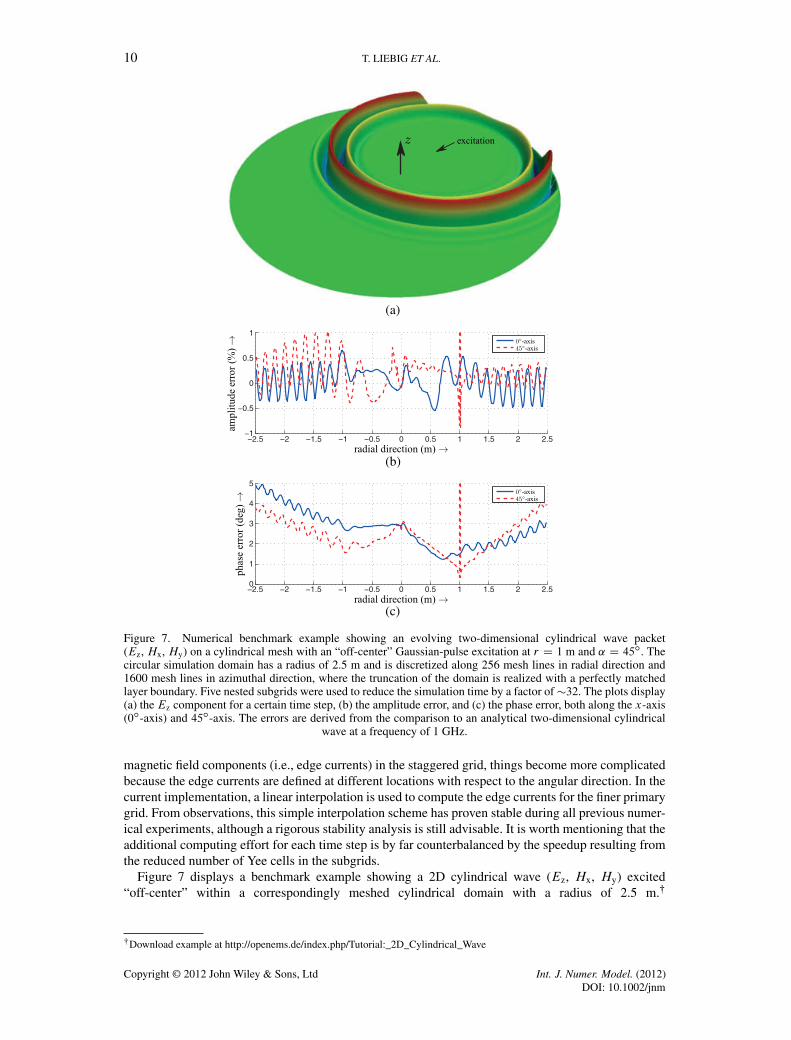
Figure 7. Numerical benchmark example showing an evolving two-dimensional cylindrical wave packet(Ez, Hx, Hy) on a cylindrical mesh with an “off-center” Gaussian-pulse excitation at r D 1 m and ˛ D 45ı. Thecircular simulation domain has a radius of 2.5 m and is discretized along 256 mesh lines in radial direction and1600 mesh lines in azimuthal direction, where the truncation of the domain is realized with a perfectly matchedlayer boundary. Five nested subgrids were used to reduce the simulation time by a factor of $32. The plots display(a) the Ez component for a certain time step, (b) the amplitude error, and (c) the phase error, both along the x-axis(0ı-axis) and 45ı-axis. The errors are derived from the comparison to an analytical two-dimensional cylindrical

wave at a frequency of 1 GHz.

magnetic field components (i.e., edge currents) in the staggered grid, things become more complicatedbecause the edge currents are defined at different locations with respect to the angular direction. In thecurrent implementation, a linear interpolation is used to compute the edge currents for the finer primarygrid. From observations, this simple interpolation scheme has proven stable during all previous numer-ical experiments, although a rigorous stability analysis is still advisable. It is worth mentioning that theadditional computing effort for each time step is by far counterbalanced by the speedup resulting fromthe reduced number of Yee cells in the subgrids.

Figure 7 displays a benchmark example showing a 2D cylindrical wave (Ez, Hx, Hy) excited“off-center” within a correspondingly meshed cylindrical domain with a radius of 2.5 m.!

!Download example at http://openems.de/index.php/Tutorial:_2D_Cylindrical_Wave



http://openems.de/index.php/Tutorial:_2D_Cylindrical_Wave


When supporting an excitation bandwidth, for example, within the spectral range of 0–2 GHz, themesh resolution has to be chosen accordingly—namely with respect to the outmost boundary of thecylindrical domain—leading to 1600 azimuthal mesh lines. This outmost boundary is actually repre-sented by a PML for the truncation of the overall simulation domain in the radial direction. To studythe scaling behavior, five subgrid stages were introduced where the resulting numerical performance isthen compared with the initial one on the basis of the full cylindrical mesh. An increase in the time stepby a factor of 31.94 was deduced from simulations, which is obviously very close to the theoreticallyachievable maximum of 25 D 32 rendering our FDTD scheme very efficient.

For further validation, we compared the 1 GHz spectral component of an evolving wave packet withthe analytical representation of a corresponding 2D cylindrical wave train. A very good agreement canbe deduced from Figure 7(b)–(c)), yielding an amplitude error (cf. Figure 7(b)) that is below 1% withinthe entire simulation domain (except at the singular excitation point). The phase error (cf. Figure 7(c))is very small as well, especially when considering that this error is still below 5ı at the furthest domainboundary where the wave has already traveled a distance of several wavelengths (& # 0:3 m). Asthe error figures also contain contributions owing to numerical dispersion, one can conclude that ourmultiple subgridding strategy is perfectly apt to retain the accuracy needed in highly efficient 3Dcomputational electromagnetics analysis.

5. A SHOWCASE IN HIGH-FIELD (7T) MAGNETIC RESONANCE IMAGING

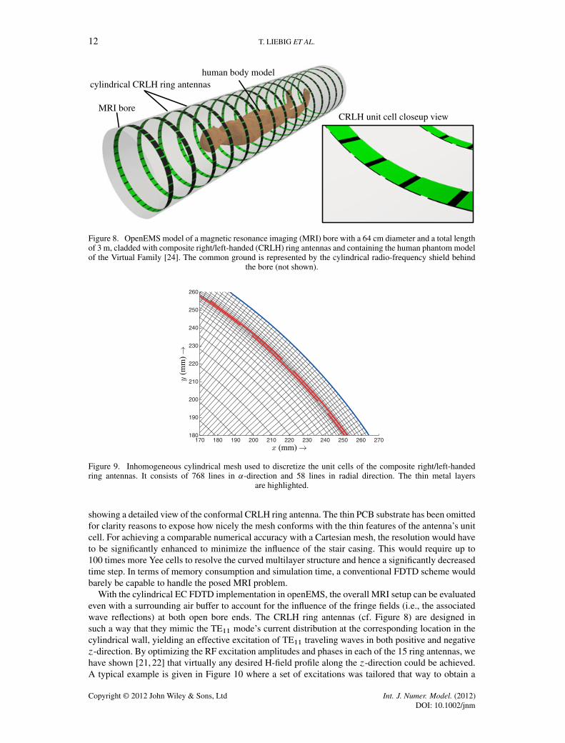
The development of the cylindrical EC FDTD algorithm has been mainly motivated by our ongoingresearch in the realm of high-field MRI [21,22]. Many devices used in this particular context confine toa cylindrical shape, such as the bore of the MRI scanner and the birdcage coils, where the latter has toconform to the cylindrical geometry within the scanner because of spatial constraints. The RF coils playan essential part in the resonant excitation of the nuclei at their corresponding Larmor frequency. TheMRI bore is surrounded by a conducting RF shield to provide a decoupling between the RF system andthe gradient coils, which are responsible for addressing the spatial information in the analyzed tissuevolume. From a distinct RF viewpoint, the MRI scanner simply boils down to a large cylindrical metalshield having a typical diameter of 64 cm and a length around 3 m. This shield encloses the patient’sbody, where the magnetic RF field is delivered and received inside the shield by using the aforemen-tioned resonant coils or antenna structures. In numerical terms, the RF system of the MRI scannerdefines a highly challenging problem, given that the large cylindrical volume may usually host struc-tures of very small and thin feature sizes. The RF aspect of the MRI scanner system is pronounced evenfurther in the framework of a novel approach that has been recently presented by Brunner et al. [19].Here, the RF magnetic field is distributed by a circularly polarized traveling TE11 wave while exploit-ing the bore’s RF shield in the very sense of a circular waveguide. To mold this traveling wave fieldaccordingly, we have proposed (following our statement in [22]) “an adaptive RF antenna system con-sisting of multiple ‘flat’ CRLH metamaterial ring antennas that fully conform to the inner surface ofthe MRI bore, and hence yields no drawback in terms of patient’s comfort” (cf. Figure 8).

A proper choice for the numerical analysis of such traveling wave MRI scenario would preferablyrely on an unstructured mesh that underlies, for example, the finite-element method, to handle the“small” conformal structures. When addressing the around one cubic meter of space inside the MRIbore together with the tiny features of a conformal CRLH antenna, finite-element method is ruled outbecause of the exceeding computational costs. In contrast, direct solvers as the FDTD method areknown to be highly memory efficient for extensive simulation domains and resolutions because thecomputational costs scale linearly with the number of cells.

Figure 8 depicts the traveling wave MRI model for the cylindrical EC FDTD simulation, where theMRI bore is populated with an equidistant arrangement of 15 conformal CRLH ring antennas. Eachring antenna consists of 32 periodic substructures (i.e., unit cells) implemented by two metal layers,which extends on both sides of a printed circuit board (PCB) substrate with a thickness of 1.28 mm(cf. inset of Figure 8). The PCB rings are then placed 10 mm apart from the ground layer representedby the cylindrical RF shield. The suitability of the graded cylindrical meshing is displayed in Figure 9



12 T. LIEBIG ET AL.

MRI bore

cylindrical CRLH ring antennashuman body model

CRLH unit cell closeup view

Figure 8. OpenEMS model of a magnetic resonance imaging (MRI) bore with a 64 cm diameter and a total lengthof 3 m, cladded with composite right/left-handed (CRLH) ring antennas and containing the human phantom modelof the Virtual Family [24]. The common ground is represented by the cylindrical radio-frequency shield behind

the bore (not shown).

170 180 190 200 210 220 230 240 250 260 270180

190

200

210

220

230

240

250

260

Figure 9. Inhomogeneous cylindrical mesh used to discretize the unit cells of the composite right/left-handedring antennas. It consists of 768 lines in ˛-direction and 58 lines in radial direction. The thin metal layers

are highlighted.

showing a detailed view of the conformal CRLH ring antenna. The thin PCB substrate has been omittedfor clarity reasons to expose how nicely the mesh conforms with the thin features of the antenna’s unitcell. For achieving a comparable numerical accuracy with a Cartesian mesh, the resolution would haveto be significantly enhanced to minimize the influence of the stair casing. This would require up to100 times more Yee cells to resolve the curved multilayer structure and hence a significantly decreasedtime step. In terms of memory consumption and simulation time, a conventional FDTD scheme wouldbarely be capable to handle the posed MRI problem.

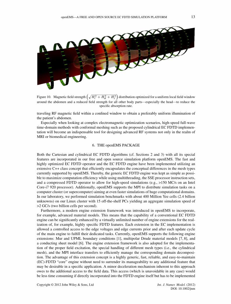
With the cylindrical EC FDTD implementation in openEMS, the overall MRI setup can be evaluatedeven with a surrounding air buffer to account for the influence of the fringe fields (i.e., the associatedwave reflections) at both open bore ends. The CRLH ring antennas (cf. Figure 8) are designed insuch a way that they mimic the TE11 mode’s current distribution at the corresponding location in thecylindrical wall, yielding an effective excitation of TE11 traveling waves in both positive and negative´-direction. By optimizing the RF excitation amplitudes and phases in each of the 15 ring antennas, wehave shown [21, 22] that virtually any desired H-field profile along the ´-direction could be achieved.A typical example is given in Figure 10 where a set of excitations was tailored that way to obtain a




Figure 10. Magnetic field strength#p

H 2r C H 2

˛ C H 2z

$distribution optimized for a uniform local field window

around the abdomen and a reduced field strength for all other body parts—especially the head—to reduce thespecific absorption rate.

traveling RF magnetic field within a confined window to obtain a preferably uniform illumination ofthe patient’s abdomen.

Especially when looking at complex electromagnetic optimization scenarios, high-speed full-wavetime-domain methods with conformal meshing such as the proposed cylindrical EC FDTD implemen-tation will become an indispensable tool for designing advanced RF systems not only in the realm ofMRI or biomedical engineering.

6. THE openEMS PACKAGE

Both the Cartesian and cylindrical EC FDTD algorithms (cf. Sections 2 and 3) with all its specialfeatures are incorporated in our free and open source simulation platform openEMS. The fast andhighly optimized EC FDTD operator and the EC FDTD engine have been implemented utilizing anextensive C++ class concept that efficiently encapsulates the conceptual differences in the mesh typescurrently supported by openEMS. Thereby, the generic EC FDTD engine was kept as simple as possi-ble to maximize computation efficiency while using multithreading, the SSE processor instruction sets,and a compressed FDTD operator to allow for high-speed simulations (e.g., >150 MC/s on an IntelCore-i7 920 processor). Additionally, openEMS supports the MPI to distribute simulation tasks on acomputer cluster (or supercomputer) aiming at even faster simulations of huge computational domains.In our laboratory, we performed simulation benchmarks with about 400 Million Yee cells (2.4 billionunknowns) on our Linux cluster with 15 off-the-shelf PCs yielding an aggregate simulation speed of>2 GC/s (two billion cells per second).

Furthermore, a modern engine extension framework was introduced in openEMS to incorporate,for example, advanced material models. This means that the capability of a conventional EC FDTDengine can be significantly enhanced by a virtually unlimited number of engine extensions for the real-ization of, for example, highly specific FDTD features. Each extension in the EC implementation isallowed a controlled access to the edge voltages and edge currents prior and after each update cycleof the main engine to fulfill their dedicated tasks. Currently, openEMS supports the following engineextensions: Mur and UPML boundary conditions [1], multipolar Drude material models [7, 8], anda conducting sheet model [6]. The engine extension framework is also adopted for the implementa-tion of the proper field excitation, the special handling of different mesh types (i.e., the cylindricalmesh), and the MPI interface transfers to efficiently manage the corresponding domain decomposi-tion. The advantage of this extension concept is a highly generic, fast, reliable, and easy-to-maintain(EC)-FDTD “core” engine without need to surrender its manageability to any additional feature thatmay be desirable in a specific application. A minor deceleration mechanism inherent to this approachowes to the additional access to the field data. This access (which is unavoidable in any case) wouldbe less time consuming if directly incorporated into the FDTD engine itself but has to be implemented



14 T. LIEBIG ET AL.

Figure 11. Three-dimensional view in the graphical user interface for openEMS (AppCSXCAD) showinga composite right/left-handed leaky wave antenna with eight unit cells. This tutorial example is available at

http://openEMS.de.

at the expense of the intended modularity. Currently, the benefits of the generic engine outweigh thisdisadvantage. For future implementations, a combined approach may become feasible if often-usedextensions (e.g., the UPML) are incorporated into the generic engines, whereas keeping other featuresas optional engine extension.

In the current implementation, OpenEMS does not rely on a highly sophisticated GUI to setup andvisualize FDTD simulation tasks as provided by most of the commercially available FDTD softwarepackages. Instead, openEMS comes with an easy-to-use Matlab interface, where even complex struc-tures are efficiently setup employing the Matlab scripting language. In addition, the user can gainaccess to all field components produced by openEMS, which allows for a high flexibility especiallywith respect to further postprocessing such as visualization. Hence, a simple GUI is made available tovisualize and review the structure in a 2D or 3D view (cf. example in Figure 11).

The Matlab interface allows to perform extensive numerical (structural) optimizations, for exam-ple, by using tailored smart search heuristics or the optimization toolbox provided by Matlab. As analternative to Matlab, the free and open source platform GNU Octave") is also recommended.

We hope to encourage and create a community who contributes new features, extensions, andenhancements to openEMS. Some of these improvements could be provided by, for example, scruti-nizing or extending the documentation, creating new tutorial examples or new (dispersive) materialmodels. Further contributions could be, for example, an enhanced and automated mesh generator orcombining openEMS with other (free) software projects, such as a circuit designer (e.g., Agilent ADS#

or Qucs‘).The complete source code, the corresponding binaries, and the installation instructions (Linux and

Windows) together with a comprehensive documentation as well with a growing collection of tutorialexamples are made available at http://openEMS.de.

"GNU Octave: http://www.gnu.org/software/octave/#Advanced Design System (ADS): www.agilent.com/find/eesof-ads‘Quite Universal Circuit Simulator: http://qucs.sourceforge.net/



http://openEMS.de

http://openEMS.de

http://www.gnu.org/software/octave/

www.agilent.com/find/eesof-ads

http://qucs.sourceforge.net/


7. CONCLUSIONS AND OUTLOOK

We have presented an EC FDTD algorithm initially for the conventional Cartesian mesh and demon-strated the high affinity of this EC FDTD formulation to a cylindrical mesh implementation, where thelatter just boils down to a different computation of the mesh specific edge lengths and cell areas. Thus,the very efficient and straightforward implementation of a generic EC FDTD engine has become pos-sible, which supports both types of meshes and was made available within our free and open sourcesimulation platform openEMS. Two special cases of the full cylindrical mesh (namely a 360ı cylin-drical mesh with and without the r D 0 singularity) have been discussed while providing solutions toboth the azimuthal round-trip wave propagation and the appropriate handling of the polar-axis singu-larity by using a particularly tailored EC FDTD operator. To address the time-stepping issue that goesalong with the decrease in cell size when progressing towards the polar-axis singularity, we showedthat it is mandatory to choose appropriate subgridding schemes to keep up with a practical simula-tion speed. Hence, the consistent use of cascaded subgrids within the cylindrical mesh enables theuser to maintain large enough time steps so that the simulation speed remains virtually unaffected bythe evolution of the cell sizes in the neighborhood of the r D 0 singularity. Compared with the cum-bersome computation within a conventional cylindrical mesh, our new subgridding strategy (i.e., thepiecewise decrement of the azimuthal grid resolution while approaching the singularity) was capableto provide a speedup by a factor of 2 for each cascaded subgrid. One of our main motivations forthe development of an efficient cylindrical EC FDTD has been addressed in Section 5 in conjunctionwith our current MRI research. Within a simulation showcase that is ideally suited to highlight theadvantage of inhomogeneous cylindrical meshing, we analyzed a very flexible traveling wave excita-tion scheme consisting of multiple conformal metamaterial ring antennas. These “flat” ring antennaswere mounted on the inner bore surface of a high-field (7T) MRI scanner, defining highly sophisti-cated features within the large bore volume. The huge size contrasts inherent to this structure are onlytractable with a FDTD scheme that supports cylindrical meshing in conjunction with multiple cas-caded subgrids. In this regard, the openEMS platform is unique compared with other FDTD packagessuch as MEEP [14] and virtually all of the commercial solvers. Especially the capabilities to createa simple structural sweep using the openEMS Matlab interface greatly supports the optimization andevaluation of the envisioned “MetaBore” concepts presented in [21, 22]. The inclusion of highly spe-cific material models with complex dispersion relations is straightforward because they just confine tocorresponding extensions assigned to the generic FDTD engine. Owing to the flexibility provided byopenEMS, the meshing and material descriptions are easily adaptable to conform applications muchdifferent than our case study, namely biological tissue and composite modeling (bioelectromagnetics),optical antennas and plasmonics (nanophotonics), and multiwalled nanotubes and nanotransmissionlines (nanoelectromagnetics). The openEMS platform is now ready for use and—above all—open tothe community to contribute many additional and exciting new engine extensions making openEMS avaluable collective venture that hopefully becomes beneficial to all dedicated users.

REFERENCES

1. Taflove A, Hagness S. Computa-tional Electrodynamics: The Finite-difference Time-domain Method,3rd edn. Artech House: Norwood,MA, 2005.

2. Kunz K. The Finite DifferenceTime Domain Method for Elec-tromagnetics. CRC Press: BocaRaton, USA, 1993.

3. Gwarek WK. Analysis of anarbitrarily-shaped planar circuit –a time-domain approach. IEEETransactions Microwave Theoryand Techniques 1985; MTT-33(10):1067–1072.

4. Craddock IJ, Railton CJ,McGeehan JP. Derivation andapplication of a passive equivalentcircuit for the finite differencetime domain algorithm. IEEEMicrowave and Guided WaveLetters 1996; 6(1):40–42.

5. Lauer A, Wolff I. Stable andefficient ABCs for graded meshFDTD simulations, IEEE MTT-SInternational Microwave Sympo-sium Digest, Vol. 2, Baltimore,MD, 1998; 461–464.

6. Lauer A, Wolff I. A conductingsheet model for efficient wideband FDTD analysis of planarwaveguides and circuits, IEEE

MTT-S International MicrowaveSymposium Digest, Vol. 4,Anaheim, CA, 1999; 1589–1592,DOI: 10.1109/MWSYM.1999.780262.

7. Rennings A, Lauer A, Caloz C,Wolf I. Equivalent Circuit (EC)FDTD Method for DispersiveMaterials: Derivation, StabilityCriteria and Application Exam-ples, Springer Proceedings inPhysics, vol. 121. Springer-Verlag:Berlin, 2008; 211–238.

8. Rennings A. Elektromagnetischezeitbereichssimulationen innova-tiver antennen auf basis vonmetamaterialien. PhD Thesis,



16 T. LIEBIG ET AL.

University of Duisburg-Essen,September 2008.

9. Weiland T. Time domain electro-magnetic field computation withfinite difference methods. Inter-national Journal of NumericalModelling: Electronic Networks,Devices and Fields July 1996;9(4):295–319.

10. van Rienen U. Numerical Methodsin Computational Electrodynam-ics – Linear Systems and PracticalApplications. Springer: Berlin,2001.

11. Rennings A, Mosig J, Caloz C,Erni D, Waldow P. Equivalentcircuit (EC) FDTD methodfor the modeling of surfacePlasmon based couplers. Journalof Computational and TheoreticalNanoscience April 2008; 5(4):690–703.

12. Rennings A, Mosig J, Gupta S,Caloz C, Kashyap R, Erni D,Waldow P. Ultra-compact powersplitter based on coupled surfacePlasmons, International Sympo-sium on Signals, Systems andElectronics, 2007. ISSSE ’07,Montréal, Québec, Canada, 2007;471–474. DOI: 10.1109/ISSSE.2007.4294515.

13. Huclova S, Erni D, Fröhlich J.Modelling effective dielectricproperties of materials contain-ing diverse types of biologicalcells. Journal of Physics D:Applied Physics September 2010;43(36):365 405–1–10.

14. Oskooi AF, Roundy D, IbanescuM, Bermel P, Joannopoulos JD,Johnson SG. MEEP: a flexiblefree-software package for electro-magnetic simulations by theFDTD method. Computer Physics

Communications January 2010;181:687–702. DOI: 10.1016/j.cpc.2009.11.008.

15. Trakic A, Wang H, Liu F,Lopez HS, Crozier S. Analy-sis of transient Eddy currentsin MRI using a cylindricalFDTD method. Applied Super-conductivity, IEEE Transactionson September 2006; 16(3):1924–1936. DOI: 10.1109/TASC.2006.874000.

16. Chi J, Liu F, Xia L, Shao T,Crozier S. An improved cylin-drical FDTD algorithm and itsapplication to field-tissue inter-action study in MRI. IEEE Tran-sactions on Magnetics February2011; 47(2):466–470. DOI: 10.1109/TMAG.2010.100098.

17. Wang H, Trakic A, Xia L, Liu F,Crozier S. An MRI-dedicated par-allel FDTD scheme. Conceptsin Magnetic Resonance Part B:Magnetic Resonance Engineering2007; 31B(3):147–161. DOI: 10.1002/cmr.b.20092.

18. Kancleris Z. Handling of singu-larity in finite-difference time-domain procedure for solvingMaxwell’s equations in cylin-drical coordinate system. IEEETransactions on Antennas andPropagation February 2008;56(2):610–613, DOI 10.1109/TAP.2007.915478.

19. Brunner DO, Zanche ND,Fröhlich J, Paska J, PruessmannKP. Travelling-wave nuclear mag-netic resonance. Nature February2009; 457:994–998.

20. Caloz C, Itoh T. ElectromagneticMetamaterials: Transmission LineTheory and Microwave Applica-tions: The Engineering Approach.

Wiley-Interscience: New York,2006.

21. Erni D, Liebig T, Rennings A,Koster NHL, Fröhlich J. Highlyadaptive RF excitation schemebased on conformal resonantCRLH metamaterial ring antennasfor 7-Tesla traveling-wave mag-netic resonance imaging, 33thAnnual International Conferenceof the IEEE Engineering inMedicine and Biology Society(IEEE EMBS 2011), Bosten, MA,USA, 2011; 554–558.

22. Liebig T, Erni D, Rennings A,Koster NHL, Fröhlich J. Meta-Bore - a fully adaptive RF fieldcontrol scheme based on confor-mal metamaterial ring antennasfor high-field traveling-wave MRI.Magnetic Resonance in Physics,Biology and Medecine (MAGMA);24:37–38. Special Supplement onthe European Society for Mag-netic Resonance in Medicineand Biology 28th Annual Sci-ence Meeting (ESMRMB 2011),paper 49 (talk and poster), pp. 22,October 6-8, Leipzig, Germany,2011.

23. Liebig T. openEMS - OpenElectromagnetic Field Solver.Available at: http://openEMS.de.[Accessed on: 10/07/2012].

24. Christ A, Kainz W, Hahn EG,Honegger K, Zefferer M, NeufeldE, Rascher W, Janka R, Bautz W,Chen J, et al. The Virtual Family– development of surface-basedanatomical models of two adultsand two children for dosimetricsimulations. Physics in Medicineand Biology January 2010; 55:N23–N38. DOI: 10.1088/0031-9155/55/2/N01.

AUTHORS’ BIOGRAPHIES:

Thorsten Liebig received his diploma degree in electrical engineering from theUniversity of Duisburg Essen in 2007. Since October 2007, he is a PhD student atthe Laboratory for General and Theoretical Electrical Engineering at the University ofDuisburg-Essen, Germany (http://www.ate.uni-due.de/). His current research includesapplied electromagnetics and electromagnetic metamaterials for applications in MRIimaging, as well as numerical methods for computational electromagnetics. He isa creator and main developer of the free and open-source equivalent-circuit FDTDsimulation platform openEMS (http://openEMS.de/).




Andreas Rennings studied electrical engineering at the University of Duisburg-Essen,Germany. He carried out his diploma work at the Microwave Electronics Laboratoryof the University of California at Los Angeles. He received his Dipl.-Ing. and Dr.-Ing.degrees from the University of Duisburg-Essen in 2000 and 2008, respectively. From2006 to 2008, he was with IMST GmbH in Kamp-Lintfort, Germany, where he workedas an RF engineer. Since then, he is a senior scientist at the Laboratory for General andTheoretical Electrical Engineering of the University of Duisburg-Essen, where he is aproject leader in the field of bioelectromagnetics and med-tech. His general researchinterests include all aspects of theoretical and applied electromagnetics, currently witha focus on medical applications. He has authored and co-authored over 60 conferenceand journal papers and one book chapter and filed eight patents. He received severalawards, including the second price within the student paper competition of the 2005

IEEE Antennas and Propagation Society International Symposium and the VDE-Promotionspreis 2009 for hisdoctoral thesis.

Sebastian Held studied electrical engineering at the University of Duisburg-Essen,Germany. He carried out his diploma work at the Institute of Microwave and RFTechnology and received his Dipl.-Ing. degree in 2004. There he worked until 2009 asa research assistant in the field of antennas and RF circuit design. In 2009, he joined theLaboratory for General and Theoretical Electrical Engineering where he was involvedin the development of active electromagnetic metamaterial antennas for automotiveapplications. Since 2011, he is with SIM Scientific Instruments Manufacturer GmbHat Oberhausen, Germany, where he works as a hardware and software engineer.

Daniel Erni received his diploma degrees from the University of Applied Sciencesin Rapperswil in 1986 and from ETH Zürich in 1990, both in electrical engineering.Since 1990, he has been working at the Laboratory for Electromagnetic Fields andMicrowave Electronics, ETH Zürich, where he obtained his PhD degree in 1996. From1995-2006, he has been the founder and head of the Communication Photonics Groupat ETH Zürich. Since October 2006, he is a full professor for General and TheoreticalElectrical Engineering at the University of Duisburg-Essen, Germany (http://www.ate.uni-due.de/). His current research includes advanced data transmission schemes(i.e., O-MIMO) in board-level optical interconnects, optical on-chip interconnects,ultra-dense integrated optics, nanophotonics, plasmonics, quantum optics, electromag-netic and optical metamaterials, and applied electromagnetics (cf. electromagneticmetamaterials for applications in MRI imaging). On the system level, he has pioneered

the introduction of numerical structural optimization into dense integrated optics device design. Further researchinterests include science and technology studies as well as the history and philosophy of science with a distinctfocus on the epistemology in engineering sciences. He is a member of the editorial board of the Journal ofComputational and Theoretical Nanoscience and edited the 2009 Special Issue on Functional Nanophotonicsand Nanoelectromagnetics. He is a fellow of the Electromagnetics Academy, a member of the Center forNanointegration Duisburg-Essen, and an associated member of the Swiss Electromagnetics Research Centre, aswell as a member of the Swiss Physical Society, the German Physical Society, the Optical Society of America,and the IEEE.



http://www.ate.uni-due.de/

http://www.ate.uni-due.de/

Documents

openEMS a free and open source equivalentcircuit (EC) … · this unwanted numerical slow-down. The performance of the cylindrical EC FDTD implementation is presented in Section 5