Open to manipulation and pro­cyclical:  a detailed analysis of Germany’s ‘debt brake’ 

Achim Truger

Berlin School of Economics and Law

and

Henner Will (†)

Macroecomomic Policy Institute (IMK) at Hans-Boeckler-Foundation, Duesseldorf, Germany

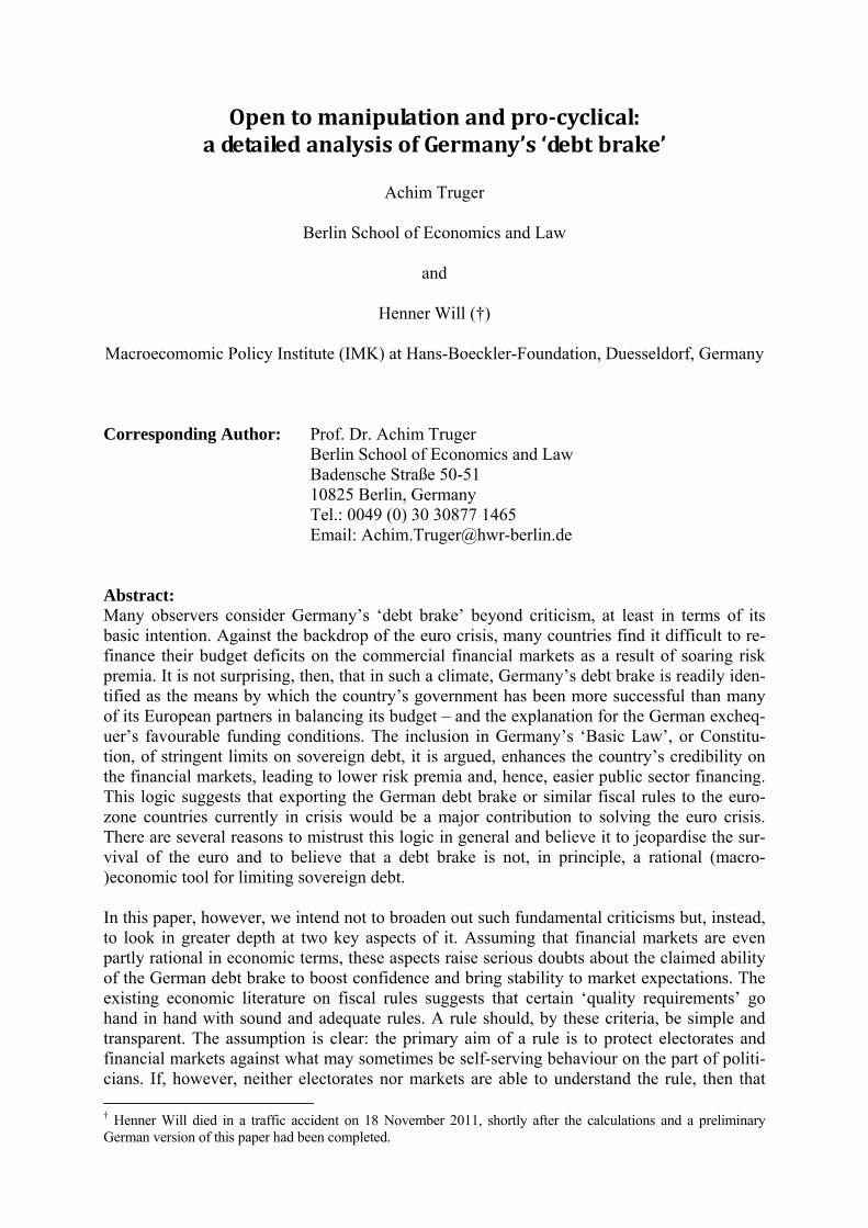
Corresponding Author: Prof. Dr. Achim Truger Berlin School of Economics and Law Badensche Straße 50-51 10825 Berlin, Germany Tel.: 0049 (0) 30 30877 1465 Email: Achim.Truger@hwr-berlin.de Abstract: Many observers consider Germany’s ‘debt brake’ beyond criticism, at least in terms of its basic intention. Against the backdrop of the euro crisis, many countries find it difficult to re-finance their budget deficits on the commercial financial markets as a result of soaring risk premia. It is not surprising, then, that in such a climate, Germany’s debt brake is readily iden-tified as the means by which the country’s government has been more successful than many of its European partners in balancing its budget – and the explanation for the German excheq-uer’s favourable funding conditions. The inclusion in Germany’s ‘Basic Law’, or Constitu-tion, of stringent limits on sovereign debt, it is argued, enhances the country’s credibility on the financial markets, leading to lower risk premia and, hence, easier public sector financing. This logic suggests that exporting the German debt brake or similar fiscal rules to the euro-zone countries currently in crisis would be a major contribution to solving the euro crisis. There are several reasons to mistrust this logic in general and believe it to jeopardise the sur-vival of the euro and to believe that a debt brake is not, in principle, a rational (macro-)economic tool for limiting sovereign debt. In this paper, however, we intend not to broaden out such fundamental criticisms but, instead, to look in greater depth at two key aspects of it. Assuming that financial markets are even partly rational in economic terms, these aspects raise serious doubts about the claimed ability of the German debt brake to boost confidence and bring stability to market expectations. The existing economic literature on fiscal rules suggests that certain ‘quality requirements’ go hand in hand with sound and adequate rules. A rule should, by these criteria, be simple and transparent. The assumption is clear: the primary aim of a rule is to protect electorates and financial markets against what may sometimes be self-serving behaviour on the part of politi-cians. If, however, neither electorates nor markets are able to understand the rule, then that † Henner Will died in a traffic accident on 18 November 2011, shortly after the calculations and a preliminary German version of this paper had been completed.

 

2

rule is not particularly useful. As we shall set out in this paper, the rule currently being ap-plied by the German government is, regrettably, neither simple nor transparent. Calculating structural deficits is a highly complex process, and since the German government has with-held some information, there has been a period when not even experts were able to make those calculations. Such calculations are also extremely sensitive to changing specifications, so outcomes are open to political manipulation. The inherently pro-cyclical nature of the German rule, and the concomitant risk of a policy that will exacerbate a crisis, are unlikely to secure the long-term confidence of the financial markets. The paper will be structured as follows. Section 2 will begin with a short account of some of the principal conceptual problems of a debt brake from a fiscal policy and macroeconomic view. Sections 3, 4 and 5 will comprise the technical detailed analysis and use the authors’ own simulated calculations to demonstrate that the methodology used by the government of the Federal Republic (the Bund) on the basis of the European Commission’s cyclical adjust-ment method is very open to manipulation and produces pro-cyclical outcomes. Section 3 will show the enormous scope for interpretation opened up by the method. Section 4 will provide an overview of how the German government is actually using the resulting margins to give itself budgetary leeway in the transitional period up to 2016. Section 5 will illustrate in detail the problem of the European Commission method’s pro-cyclical susceptibility to revision. A dynamic simulation will provide the first explicit illustration of the budget balancing method for two economic scenarios explicitly linked to the authors’ own tax revenue estimates, to demonstrate the impact of the debt brake on budget targets during the transitional period up to 2016. It will show that the margins that appear currently to exist will be progressively eroded by any downturn in the economy. Ultimately, further discretionary consolidation measures beyond the government’s plan to cut spending – its ‘Future Package’ – will be required to meet the targets set out under the debt brake. Section 6 will finally draw some brief conclu-sions.

 

3

Open to manipulation and pro-cyclical: a detailed analysis of Germany’s ‘debt brake’

Achim Truger and Henner Will

1. Introduction

Many observers consider Germany’s ‘debt brake’ beyond criticism, at least in terms of its

basic intention. Against the backdrop of the euro crisis, many countries still find it increas-

ingly difficult to refinance their budget deficits on the commercial financial markets as a re-

sult of soaring risk premia. Add that to the disastrous economic and social impact of the aus-

terity policies their governments are imposing, and you have the perfect conditions for esca-

lating anxiety about sovereign debt. It is not surprising, then, that in such a climate, Ger-

many’s debt brake is readily identified as the means by which the country’s government has

been more successful than many of its European partners in balancing its budget – and the

explanation for the German exchequer’s favourable funding conditions. The inclusion in

Germany’s ‘Basic Law’, or Constitution, of stringent limits on sovereign debt, it is argued,

enhances the country’s credibility on the financial markets, leading to lower risk premia and,

hence, easier public sector financing (see Heinemann et al. 2011). This logic suggests that

exporting the German debt brake or similar fiscal rules to the eurozone countries currently in

crisis would be a major contribution to solving the euro crisis (see GD 2011, p. 51). We con-

sider that logic to be fundamentally flawed and believe that it would jeopardise the survival of

the euro for three major reasons. First, it is misleadingly reductive in tracing the cause of the

euro crisis back to unstable fiscal policy in the countries currently experiencing difficulties.

Second, it almost completely ignores the effect of imbalances in foreign trade and the respon-

sibility of the eurozone countries that are (still) currently strong in economic terms. Third, it

remains bizarrely attached to the long-discredited assumption that financial markets are ra-

tional (see Horn et al. 2010a, 2010b, 2011a, 2011b, 2011c; IMK/OFCE/WIFO 2011). We also

believe that a debt brake is not, in principle, a rational (macro-)economic tool for limiting

sovereign debt (see Horn et al. 2008, 2009; Truger/Will 2009; Truger et al. 2009, 2011; Horn

et al 2011a).

In this paper, however, we intend not to broaden out this fundamental criticism but, instead, to

look in greater depth at two key aspects of it. Assuming that financial markets are even partly

rational in economic terms, these aspects raise serious doubts about the claimed ability of the

German debt brake to boost confidence and bring stability to market expectations. The exist-

ing economic literature on fiscal rules suggests that certain ‘quality requirements’ go hand in

 

4

hand with sound and adequate rules. A rule should, by these criteria, be simple and transpar-

ent (see Kopits/Symanski 1998). The assumption is clear: the primary aim of a rule is to pro-

tect electorates and financial markets against what may sometimes be self-serving behaviour

on the part of politicians. If, however, neither electorates nor markets are able to understand

the rule, then that rule is not particularly useful. As we shall set out in this paper, the rule cur-

rently being applied by the German government is, regrettably, neither simple nor transparent.

Calculating structural deficits is a highly complex process, and since the German government

has withheld some information, there has been a period when not even experts were able to

make those calculations. Such calculations are also extremely sensitive to changing specifica-

tions, so outcomes are open to political manipulation. The inherently pro-cyclical nature of

the German rule, and the concomitant risk of a policy that will exacerbate a crisis, are unlikely

to secure the long-term confidence of the financial markets.

The paper is structured as follows. Section 2 begins with a short account of some of the prin-

cipal conceptual problems of a debt brake from a fiscal policy and macroeconomic view. Sec-

tions 3, 4 and 5 comprise the technical detailed analysis and use the authors’ own simulated

calculations to demonstrate that the methodology used by the government of the Federal Re-

public (the Bund) on the basis of the European Commission’s cyclical adjustment method is

very open to manipulation and produces pro-cyclical outcomes. Section 3 shows the enor-

mous scope for interpretation opened up by the method. Section 4 then provides an overview

of how the German government is actually using the resulting margins to give itself budgetary

leeway in the transitional period up to 2016. Section 5 illustrates in detail the problem of the

European Commission method’s pro-cyclical susceptibility to revision. A dynamic simulation

provides the first explicit illustration of the budget balancing method for two economic sce-

narios explicitly linked to the authors’ own tax revenue estimates, to demonstrate the impact

of the debt brake on budget targets during the transitional period up to 2016. It shows that the

margins that appear currently to exist will be progressively eroded by any downturn in the

economy. Ultimately, further discretionary consolidation measures beyond the government’s

plan to cut spending – its ‘Future Package’ – will be required to meet the targets set out under

the debt brake. Section 6, finally, draws some brief conclusions.

 

5

2. Fundamental problems of the debt brake from a fiscal policy and macroeconomic

perspective

2.1 The key characteristics of Germany’s debt brake

The debt brake written into Germany’s Constitution in 2009 essentially comprises three ele-

ments. The structural component imposes strict limits on structural government deficits –

0.35% of GDP for the federal level (the Bund) and 0.0% for the federal states or Länder. The

cyclical component increases or decreases these limits in accordance with the country’s eco-

nomic situation. An exception clause, finally, permits the rules to be broken in exceptional

circumstances. The Bund also has an ‘adjustment account’, which ensures the debt brake ap-

plies not only when the country’s budget is drawn up but also when it is implemented. Transi-

tional periods for complying with these limits on structural debt are written into the legisla-

tion: 2016 for the Bund and 2020 for the Länder. The legislation also provides for consolida-

tion aid for five Länder (Berlin, Bremen, Saarland, Saxony-Anhalt, and Schleswig-Holstein),

which imposes strict constraints. The debt brake targets, in fact, go a little further than is nec-

essary to enable Germany to meet its medium-term national budget targets: under the preven-

tive arm of the European Growth and Stability Pact, Germany is allowed a structural deficit

equivalent to 0.5% of GDP.

2.2 Fundamental problems with the debt brake from a fiscal policy and macro-

economic perspective

We shall not go into the detail of Germany’s fiscal policy before the debt brake was intro-

duced. Suffice it to say that this policy has been traditionally pro-cyclical for more than 30

years and that between 2000 and the crisis in 2009, its dangerous mix of continual tax cuts

and the rigid pursuit of a balanced budget caused severe damage to growth and employment,

substantially widened existing inequalities in income distribution, and weakened the country’s

public finances (Truger 2004, 2009, 2010; Truger/Teichmann 2011). There was, therefore,

good reason for a change of course. However, the change of course represented by the debt

brake can be criticised on at least five grounds.

First, the capping – now anchored in the German Constitution – of structural government net

borrowing at 0.35% of GDP for the Bund and the banning of all structural deficits by the

Länder is, economically speaking, completely arbitrary. It means that with average annual

growth in nominal GDP of 3%, the long-term result is a national debt-to-GDP ratio of just

11.7%. We do not contest that there are arguments for some ceiling on the debt ratio, but re-

 

6

cent empirical research indicates that the critical threshold beyond which a government deficit

can harm growth is 80% or even 90%.2 We fear that by imposing artificial limits on what is

traditionally the safest form of investment, the debt brake will instead deprive capital markets

of a crucial stability factor and a vital benchmark. It is unclear into which forms of invest-

ment, and to which countries, the traditionally high excess savings of the German private sec-

tor (including the assets of private pension schemes) will be diverted in future, but it is likely

that this measure will render the financial markets considerably less stable in the long term.

Second, by using a debt brake, Germany’s fiscal policy is ignoring a broadly accepted eco-

nomic yardstick for the scale of national deficits – the ‘Golden Rule’ – and thus turning its

back on 60 years of theoretical common sense. This Golden Rule, or the ‘pay-as-you-use’

principle, is a growth-oriented rule for new borrowing that permits new structural borrowing

beyond the cycle equivalent to net public investment. The idea behind the rule is to involve

several generations in financing public capital accumulation, since future generations will

benefit in terms of greater prosperity from the productive investments made now (see Mus-

grave 1959; SVR 2007). It is true that the old rules governing borrowing by both the Bund

and the Länder in the constitution were imperfect: they were unable to distinguish between

gross and net investment and, moreover, they failed to include all forms of economically rele-

vant investment. However, there was no discussion around a more workable definition or an

estimate of depreciation – just as there was not with the Maastricht criteria or the European

Stability and Growth Pact – and the government ignored recommendations made by the

Council of Economic Experts (SVR 2007), a body not exactly known to endorse runaway

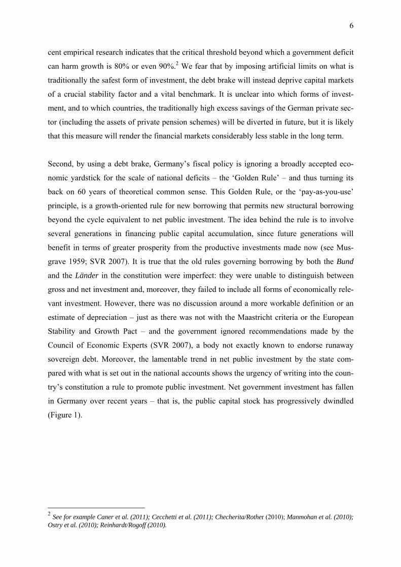
sovereign debt. Moreover, the lamentable trend in net public investment by the state com-

pared with what is set out in the national accounts shows the urgency of writing into the coun-

try’s constitution a rule to promote public investment. Net government investment has fallen

in Germany over recent years – that is, the public capital stock has progressively dwindled

(Figure 1).

2 See for example Caner et al. (2011); Cecchetti et al. (2011); Checherita/Rother (2010); Manmohan et al. (2010); Ostry et al. (2010); Reinhardt/Rogoff (2010).

 

7

Figure 1: government net investment in billion EUR and in % of GDP,

Germany (1980-2010)

Source: AMECO (autumn 2010)

Third, possibly the most serious problem associated with the debt brake is that it was intro-

duced at a time when public budgets were markedly underfinanced in structural terms, as they

have for many years come under repeated strain from tax cuts. The long-term tax reductions

adopted in the wake of the global economic and financial crisis and Germany’s ‘Growth Ac-

celeration Act’ were in the dimension of almost EUR 30 billion a year (Truger/Teichmann

2011). Where the governments are expected to balance its budget in structural terms – or to

come very close to doing so – on a given date without already having closed the revenue gap,

their budget policy faces years of stringent pressure on spending. In macroeconomic terms,

this is an extremely risky course of action with potentially negative impact on growth and

employment as adjustments are made, including – and particularly – against the backdrop of

the precarious economic situation in the eurozone as a whole, and it will unquestionably go

hand in hand with substantial cuts in the provision of public goods, services and welfare. And

if this then leads (as it almost inevitably will) to the necessary central investment being

scrapped or cut in future years, the much-vaunted principle of ‘generational fairness’ is

greatly damaged. Moreover, substantial spending cuts cannot be justified because expenditure

policy in the past has been wasteful: On the contrary, the debt brake affects German public

sector budgets after a period of extremely moderate expenditure growth (Truger/Teichmann

2011). The decision taken jointly by both houses of the German parliament to implement the

debt brake and couple it for a limited period with generous, long-term tax relief (including the

reinstatement of tax relief on their journey to work for commuters, the two-stage reduction in

 

8

the rate of income tax, the ‘Citizen Relief Act’ – which makes contributions to health insur-

ance schemes tax-deductible – and the so called Growth Acceleration Act) was, therefore,

worse than negligent in terms both of economic impact and of national policy. For these rea-

sons alone, it would have been sensible from a macroeconomic stance – but ultimately also in

budgetary terms – not to anchor the debt brake in Germany’s Constitution.

There are two further areas of criticism, and this paper explores those in greater detail.

Fourth, the impact of the debt brake is also, of course, critically dependent on its precise tech-

nical design and on how the underlying cyclical adjustment method and the applicable budget

sensitivities are selected. Although the Bund has already opted for the method used by the

European Commission as part of its own budget monitoring, the decision as to the details of

implementation is taken by the Ministries for Finance and Economics, so the mechanism is

anything but transparent and is open to manipulation. As far as the Länder are concerned, for

many of them implementation is still an open question. And since, under Article 109 of the

Basic Law, there is considerable scope for local input, Germany could by 2020 have no fewer

than 17 different debt brakes, one for the Bund and one for each of the Länder, all with widely

differing designs and effects.

Fifthly, and finally, the debt brake will ultimately have a pro-cyclical effect because of the

way the commonly used cyclical adjustment method works and will, as a result, destabilise

economic development. During times of downturn, too much consolidation will be required

while, conversely, too little will be required during periods of recovery.

The last two areas of criticism will be explored in greater detail in this paper.

3. Vulnerability to manipulation in theory: the problem of determining structural

deficits

3.1 Introduction to determining structural deficits

The debt brake provides for public sector budgets to breathe with the economy; in other

words, the automatic stabilisers must be allowed to operate freely. A calculation therefore

needs to be made as to which changes in the deficit can be attributed solely to cyclical factors

and, hence, the automatic stabilisers, and which part of the deficit is structural and must,

therefore, be capped under the debt brake. When a cyclical adjustment method is used, this

usually determines the notional economic situation (output potential or output trend). The

mismatch between this notional situation and the actual situation is known as the ‘output gap’.

Where this is positive, the state of the economy dictates that surpluses are achieved, but where

 

9

it is negative, economic deficits are permitted. The calculation of the scale of the permissible

deficit or surplus is then based on the product of the output gap and the budget sensitivity.

The latter reflects the impact of changes in the economic cycle on the government budget and

is calculated empirically (Girouard/André 2005). The structural deficit is then calculated after

deducting the previously calculated the cyclical deficit.

Germany’s Ministry of Finance follows the following specific formula in calculating the Fed-

eral Republic’s debt brake:

(1)

The structural deficit as a percentage of potential nominal GDP is, therefore,

the total deficit (revenue minus expenditure ) set against potential nominal GDP

minus the cyclical deficit, which in turn is the product of elasticity of revenue ( ) and elas-

ticity of expenditure ( ) of the automatic stabilisers (budget sensitivity) and of the nominal

output gap .

However, there are many possible ways of calculating output gap and budget sensitivity, and

these produce radically divergent results in terms of calculating the structural deficit and,

hence, determining budgetary policy. Determining output potential has already proved both

difficult and unreliable (Horn et al. 2007). As well as univariate methods, such as the

Hodrick-Prescott filter –proposed by the Council of Economic Experts – and the modified

Hodrick-Prescott filter, which is used in Switzerland (Bruchez 2003), a wide range of diverse

multivariate estimation methods are also available, such as that used by the European Com-

mission.

3.2 The European Commission’s method for determining potential

Germany’s legislation implementing the debt brake –the Article 115 Act – has opted “by

means of a statutory instrument and without the consent of the Bundesrat, [to] stipulate the

details of the procedure for determining the cyclical component in conformity with the cycli-

cal adjustment method applied within the framework of the European Stability and Growth

Pact. The procedure shall be reviewed and developed further on a regular basis taking the

current state of knowledge into account.”3

The European Commission estimates output potential by means of a Cobb-Douglas-

production function. This is derived from potential labour input (the product of the working

3 Para. 5(4) of Article 115 of the law of 10 August 2009 (German Federal Gazette (BGBl.) I, pp.2702 and 2704)

 

10

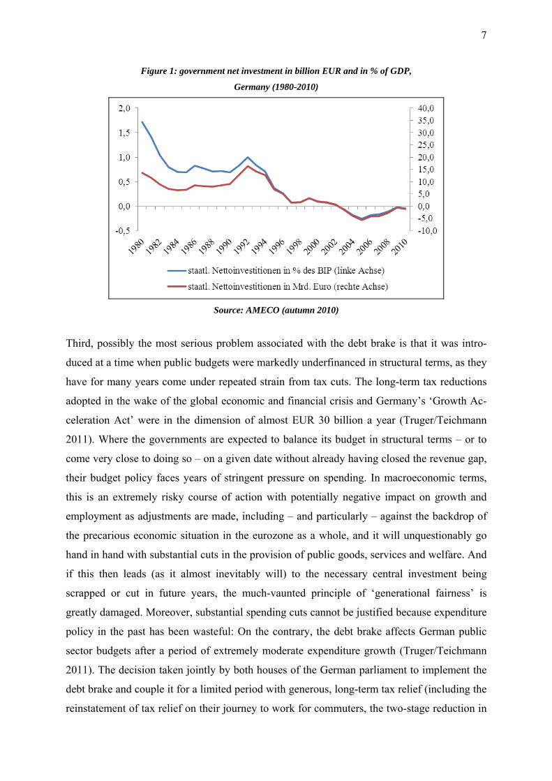
age population, the participation rate and per capita hours of work minus structural unem-

ployment), capital input (the product of the gross investment rate of the potential and the po-

tential minus a constant depreciation) and total factor productivity or TFP (in the former

method, this was expressed as a Solow residual with Hodrick-Prescott filtering, while in the

new process, it is expressed as Kalman-filtered capacity utilisation) (see D’Auria et al. 2010).

The individual elements can be portrayed formally as follows:

(2)

(3)

(4)

with YPOT as the output potential, LPOT as the labour potential, K as capital accumulation, TFP

as the total factor productivity, BEA as working age population, E as employees, U as the

unemployed, (E+U)/BEA as the participation rate, NAWRU as the non-accelerating wage rate

of unemployment, H/E as per capita hours of work, I/YPOT as the gross asset investment ratio

related to output potential, and δ as the rate of depreciation.

The estimate of potential is a medium-term projection based on short-term forecasts (one to

two years). All the elements in the formulae used are forecast separately: demographic trends,

the participation rate, structural unemployment, per capita hours of work, the investment ratio,

the rate of depreciation (usually a constant), and the TFP, either as a filtered Solow residual or

as Kalman-filtered capacity utilisation. The model solution is derived using statistical soft-

ware. The estimate is calculated for all EU Member States using semi-standardised specifica-

tions but with different details. The specifications are normally adjusted every six months.

3.3 The “current state of knowledge”4

The formulation “in conformity with” used in the Article 115 Act suggests at first glance that

the German government is applying the European Commission’s method very precisely.

Comparison with the “current state of knowledge” shows, however, that the government has

in fact left itself a generous margin for interpretation. However, even if it were to comply to

the letter with the European Commission method, this would not shed much light on what is

actually happening: in 2010, the Commission itself amended its calculation method twice in

twelve months (Table 1). First, in its spring forecast, it outlined a modified method (III – new

TFP, spring), which identifies total factor productivity as less sensitive to cyclical factors than 4 The analysis below is based on calculations similar to those already outlined in Horn et al. (2011a).

 

11

under the old method (I – old TFP, spring). However, in its autumn forecast, the European

Commission made a further modification to the new method (IV – new TFP, autumn), in

which the variables represented by the participation rate and per capita hours of work were

adjusted. Despite this, it also reflected the old method in its autumn modifications (II – old

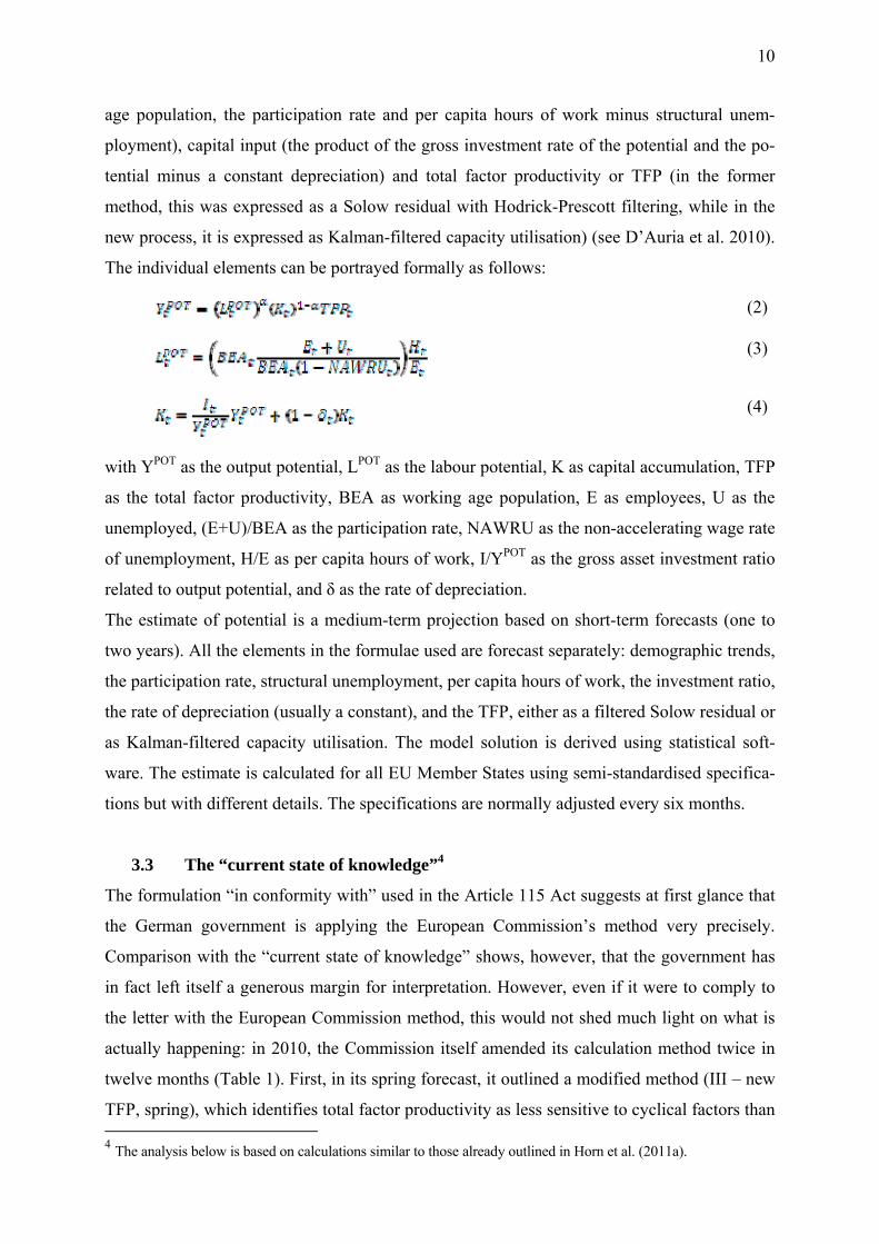
TFP, autumn). This means that for 2010, a key year in terms of determining the adjustment

path to the final structural deficit target in 2016, there were no fewer than four different EU

methods for cyclical adjustment. Accordingly, for any given budget sensitivity, four cyclical

components and correspondingly four structural deficits could be calculated, each with a

markedly different impact on budget policy.

Table 1: Descriptions of the EU Commission methods 2010

EU Commission Methods

No. Description changes from I

I old method ,

spring version

–

II old method,

autumn version

Per-capita-working hours with slightly descreasing trend, slight decrease in

participation

III new method,

spring version

Exogenous estimation of total factor productivity

IV new method,

autumn version

Exogenous estimation of total factor productivity; Per-capita-working hours

with slightly descreasing trend, slight decrease in participation

Source: EU Commission

The impact of these four different methods of calculation should not be underestimated. With

total net borrowing of EUR 44.8 billion, and assuming a budget sensitivity of 0.248, the 2010

structural component ranges from EUR 19 billion to EUR 35 billion, depending on the

method and the version applied (Table 3, reference scenarios).

The output gap and cyclical component values calculated by the German government in for-

mulating its 2011 budget do not match any of these values, even though the assumptions relat-

ing to growth were compatible with those of the European Commission. Without providing

detailed data relating to its assumptions, the German government announced an output gap for

2011 of -0.6% of GDP (using the old EU method) and a cyclical component of EUR -2.5 bil-

lion. These figures were, thus, outside the range of estimates produced by the four versions of

the European Commission method, showing that the government did not slavishly apply any

 

12

version of the European Commission method(s).

In fact, there is considerably greater scope for further modification. The Joint Economic Fore-

cast in autumn 2010 did exactly that, making explicit reference to the European Commission

method, though unfortunately not applying it transparently (GD 2010, p.44). Although the

Joint Economic Forecast results cannot be reproduced because some data have been withheld,

the changes that have been published can be interpreted as in line with the “current state of

knowledge”. Thus, we introduce similar modifications and the estimates calculated for output

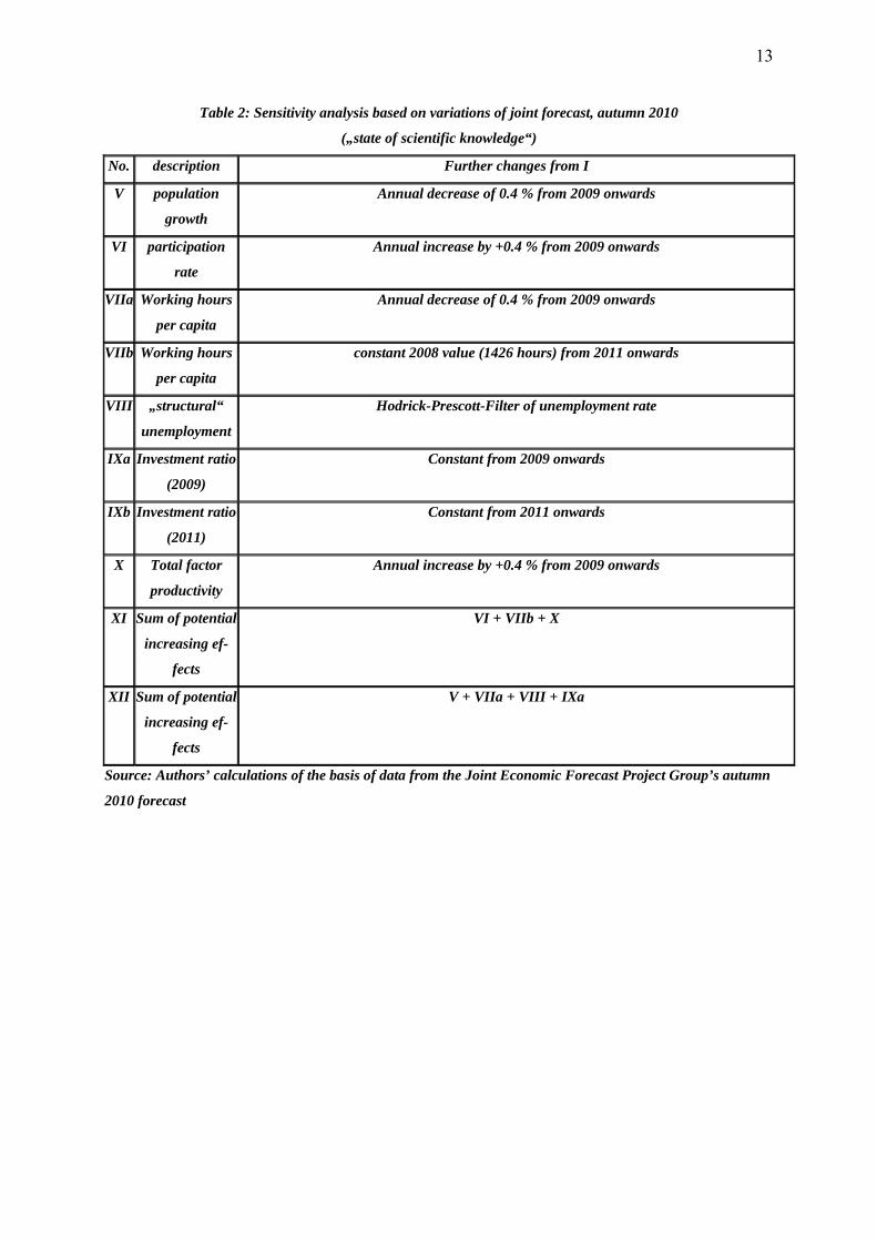
gap and structural deficit can be regarded as permissible under the German debt brake. Table

2 contains details of the modifications, while Table 3a reproduces the output gaps and Table

3b the structural deficits. First, the data for the four reference ranges from Table 1 are listed,

with a distinction made between two different datasets (spring and autumn). Then each refer-

ence is modified in accordance with the changes in Table 2 and the new calculation – again,

differentiated according to dataset – is presented. This produces a total of eight modifications,

four calculation methods and two datasets (4 x 2 x 8), or 64 different figures for output gap

and structural deficit. To these must be added the eight unmodified reference ranges (4 x 2 =

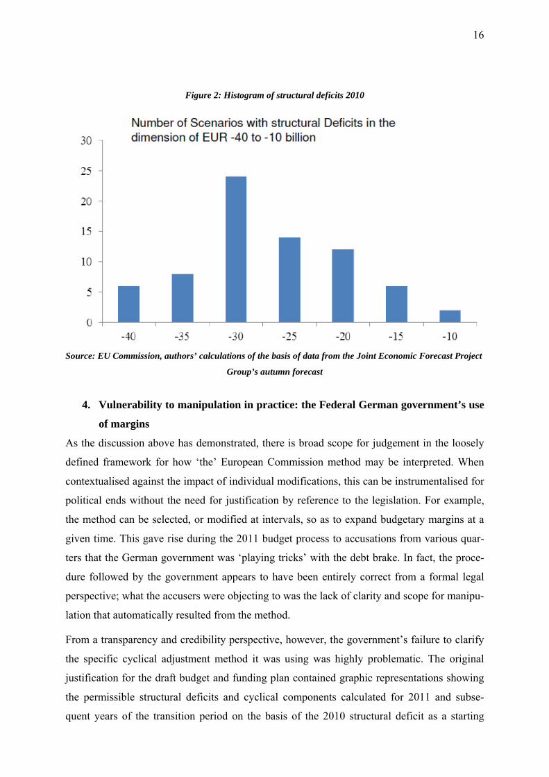
8), resulting in a total of 72 different structural deficits. Figure 2, finally, illustrates the distri-

bution of the structural deficits. These calculations show that, assuming actual net borrowing

of EUR 44.8 billion, the structural component of the budget deficit ranges from EUR -44 bil-

lion to EUR -13 billion, with a mean of EUR -30 billion. Obviously, this is anything but a

precise method.

 

13

Table 2: Sensitivity analysis based on variations of joint forecast, autumn 2010

(„state of scientific knowledge“)

No. description Further changes from I

V population

growth

Annual decrease of 0.4 % from 2009 onwards

VI participation

rate

Annual increase by +0.4 % from 2009 onwards

VIIa Working hours

per capita

Annual decrease of 0.4 % from 2009 onwards

VIIb Working hours

per capita

constant 2008 value (1426 hours) from 2011 onwards

VIII „structural“

unemployment

Hodrick-Prescott-Filter of unemployment rate

IXa Investment ratio

(2009)

Constant from 2009 onwards

IXb Investment ratio

(2011)

Constant from 2011 onwards

X Total factor

productivity

Annual increase by +0.4 % from 2009 onwards

XI Sum of potential

increasing ef-

fects

VI + VIIb + X

XII Sum of potential

increasing ef-

fects

V + VIIa + VIII + IXa

Source: Authors’ calculations of the basis of data from the Joint Economic Forecast Project Group’s autumn

2010 forecast

 

14

Table 3a:Output gap estimates for 2010

I - Old TFP Spring II - Old TFP Autumn III -New TFP Spring IV – New TFP Autumn Reference, Spring data

-2.65 -2.40 -3.86 -3.62 Reference, autumn data

-1.47 -1.34 -1.82 -1.69

Modification V, Spring data -2.65 -2.4 -3.86 -3.62

Modification V autumn data -1.21 -1.08 -1.57 -1.44

Modification VIa Spring data -2.65 -2.66 -3.86 -3.87

Modification VIa autumn data -1.47 -1.48 -1.82 -1.83

Modification VIb Spring data -2.37 -2.36 -3.59 -3.58

Modification VIb autumn data -1.12 -1.11 -1.48 -1.47

Modification VII Spring data -2.52 -2.26 -3.74 -3.48

Modification VII autumn data -1.56 -1.44 -1.92 -1.8

Modification VIII – Spring data -2.12 -1.87 -3.34 -3.09

Modification VIII autumn data -0.57 -0.44 -0.93 -0.8

Modification IX Spring data -2.65 -2.4 -3.86 -3.62

Modification IX autumn data -1,47 -1,34 -1,82 -1,69

Modification X Spring data -1,84 -1,83 -3,06 -3,05

Modification X autumn data 0,04 0,04 -0,32 -0,32

Modification XI Spring data -3,52 -3,28 -4,74 -4,49

Modification XI autumn data -1,94 -1,81 -2,61 -2,48

Source: EU Commission, authors’ calculations of the basis of data from the Joint Economic Forecast Project

Group’s autumn forecast

 

15

Table 3b: Structural deficits 2010

I – Old TFP Spring II - Old TFP Autumn III – New TFP Spring IV - New TFP Autumn Reference, Spring data

-27.14 -28.77 -19.13 -20.74 Referenz. Autumn data

-34.76 -35.59 -32.52 -33.35

Modification V Spring data -27.1 -28.8 -19.1 -20.7

Modification V Autumn data -36.4 -37.2 -34.1 -35.0

Modification VIa Spring data -27.1 -27.1 -19.1 -19.1

Modification VIa Autumn data -34.8 -34.7 -32.5 -32.5

Modification VIb Spring data -29.0 -29.0 -20.9 -21.0

Modification VIb Autumn data -37.0 -37.0 -34.7 -34.8

Modification VII Spring data -28.0 -29.7 -19.9 -21.7

Modification VII Autumn data -34.2 -35.0 -31.9 -32.6

Modification VIII Spring data -30.6 -32.2 -22.6 -24.3

Modification Autumn data -40.4 -41.3 -38.2 -39.0

Modification IX Spring data -27.1 -28.8 -19.1 -20.7

Modification IX Autumn data -34.8 -35.6 -32.5 -33.4

Modification X Spring data -32.4 -32.5 -24.4 -24.5

Modification X Autumn data -44.2 -44.2 -42.0 -42.0

Modification XI Spring data -21.4 -23.0 -13.2 -14.9

Modification XI Autumn data -31.7 -32.6 -27.4 -28.2

Source: EU Commission, authors’ calculations of the basis of data from the Joint Economic Forecast Project

Group’s autumn forecast

 

16

Figure 2: Histogram of structural deficits 2010

Source: EU Commission, authors’ calculations of the basis of data from the Joint Economic Forecast Project

Group’s autumn forecast

4. Vulnerability to manipulation in practice: the Federal German government’s use

of margins

As the discussion above has demonstrated, there is broad scope for judgement in the loosely

defined framework for how ‘the’ European Commission method may be interpreted. When

contextualised against the impact of individual modifications, this can be instrumentalised for

political ends without the need for justification by reference to the legislation. For example,

the method can be selected, or modified at intervals, so as to expand budgetary margins at a

given time. This gave rise during the 2011 budget process to accusations from various quar-

ters that the German government was ‘playing tricks’ with the debt brake. In fact, the proce-

dure followed by the government appears to have been entirely correct from a formal legal

perspective; what the accusers were objecting to was the lack of clarity and scope for manipu-

lation that automatically resulted from the method.

From a transparency and credibility perspective, however, the government’s failure to clarify

the specific cyclical adjustment method it was using was highly problematic. The original

justification for the draft budget and funding plan contained graphic representations showing

the permissible structural deficits and cyclical components calculated for 2011 and subse-

quent years of the transition period on the basis of the 2010 structural deficit as a starting

 

17

point. However, there were no concrete data relating to the method used; not even the term

‘budget sensitivity’ featured, let alone explanations of how it was determined. The govern-

ment belatedly, and at the urging of some of the MPs on the Budget Committee, provided

some additional information, yet even here – as Section 3 makes clear – the information was

decidedly thin on detail.

The conversion of the funding to the German Labour Agency (Bundesagentur für Arbeit),

from a loan to a direct, non-repayable grant in 2010 was deliberate manipulation to widen the

budgetary scope, originally with the aim of implementing as fully as possible the tax cuts set

out in the coalition agreement. A loan would have been deficit-irrelevant under the debt

brake, since the payment to the agency would have been offset by a corresponding asset – the

claim on the agency. However, converting that loan into a grant increased the actual 2010

deficit and, hence, also increased the structural deficit for the year. This structural deficit was

then used to calculate the permissible deficit for each year in the transitional period, during

which the deficit must be reduced by equal stages of one sixth of the initial value each year

until, in 2016, the deficit has been reduced to the permissible maximum of 0.35% of GDP

(around EUR 10 billion). This adroit increase in the base value for the deficit increased the

starting point for this chain of reductions, also allowing higher permissible structural deficits

during the transitional period (something referred to by some critics as the ‘ski jump effect’).

Meanwhile, the higher 2010 deficit then disappeared automatically in 2011 because of the

way the funding was designed and without any real measures to balance the budget being

necessary.

The margins created by this manipulation have now all but disappeared for two reasons. First,

favourable employment trends mean that the Bundesagentur für Arbeit’s funding requirement

has fallen from more than EUR 16 billion to just EUR 6.9 billion. Second, the government

has designed its measures to reflect budget sensitivities very consistently by setting a higher

value of 0.248 for 2010, which also included that part of the cyclical components accounted

for by the Bundesagentur für Arbeit, whereas for subsequent years, the value was a lower

0.16, which related solely to the budget of the Bund. The resulting higher cyclical component

for 2010 reduced the initial structural deficit by just over EUR 4 billion, so the residual higher

base value is minimal. Moreover, the government reduced that higher base value by using the

permissible – but unconventional – statistical device of recording one-off revenue from auc-

tions of mobile telephony licences (over EUR 4 billion) as a “structural deficit reduction”.

This, at least, was not a repeat of the ‘ski jump effect’, although this does not change the fact

that the German government originally tried to use exactly that device and other accounting

 

18

tricks to create budgetary margins for its planned fiscal policy.

In fact, the ‘ski jump effect’ did then operate in another context. In its 2011 budget, the gov-

ernment set its tax revenue estimates and the overarching calculation of cyclical components

and structural deficits against the upturn in the economy – but not the corresponding estimates

for 2010. In strict legal terms, it was not required to, but this is a loophole in the rules, which

omit to specify how, when, and on the basis of precisely which data the initial structural defi-

cit for 2010 is determined. This trick enabled the government not just to comply fully with the

debt brake in its 2011 targets but actually to overshoot it by just under EUR 5 billion.

One further curious fact was that, by its own admission, the government had used the old EU

method for its 2011 budget calculations, since – it claimed – it was unable to move to the new

method for technical reasons. That is more than improbable, given that the new method had

been in the public domain since spring 2010, and once the European Commission had put the

details online, moving over to the autumn version of it would have taken a few hours or one

working day at most. Following identification of the basic parameters for the 2012 national

budget, the government then gained further room for manoeuvre by belatedly moving its cal-

culation of the output gap to the new EU method, resulting in an increase in the estimated

negative output gap for 2011 from 0.6% of GDP to 1.0% of GDP, even though at the same

time the 2011 GDP growth forecast was itself increased from 1.8% to 2.3%. This switch of

method meant, paradoxically, that the upturn in the economy produced a marked increase in

that part of the deficit permissible on cyclical grounds.

Overall, then, the past conduct of the German government clearly confirms suspicions that

using such a technically complex method virtually inevitably produces a lack of transparency

and scope for manipulation. Although the Ministry of Finance (BMF) eventually published its

data and results following persistent criticism from spring 20115, it still falls well short of

achieving the transparency demonstrated by the European Commission, which publishes the

entire scheme for its calculations, including datasets, online. As far as exploiting the ‘ski jump

effect’ is concerned, the government failed to make a retrospective correction, despite mas-

sive protests by influential institutions including the Council of Economic Experts and the

Bundesbank (see SVR 2010; Deutsche Bundesbank 2011), an apparently justifiable decision,

given the associated negative macroeconomic and public finance effects (IMK/OFCE/WIFO

2011), although not exactly a model of transparent and credible implementation of fiscal

rules. 5http://www.bundesfinanzministerium.de/nn_4322/DE/Wirtschaft__und__Verwaltung/Finanz__und__Wirtschaftspolitik/Wirtschaftspolitik/1103311a7001.html?__nnn=true

 

19

5. The risk of pro-cyclical policy

5.1 The underlying problem of all deficit rules: budget deficits are endogenous

and mostly immune to political control

The debt brake sets a ceiling on structural deficits of 0.35% for the Bund and of 0.0% for the

Länder. As in the Stability and Growth Pact, these ceilings are tied to binding targets for defi-

cits as a percentage of economic output. This can be summarised in the following simple

mathematical formula:

const.deficitett

YA)(YE

Deficitt

tttt ==

−= arg

(5)

We shall, for the moment, leave aside the question of whether this target deficit is a general

one or a structural one – that is, whether it has been adjusted for cyclical factors. What is

more important is the functional dependence of revenue (E) on economic output (Y), while

expenditure (A) is less markedly dependent and, therefore, not portrayed as functionally de-

pendent.

During an economic upturn (when Y increases), there are two main effects. First, the denomi-

nator of the fraction rises and so the deficit falls automatically when revenue and expenditure

reach a certain level. Second, however, state revenue in particular rises, so when expenditure

reaches a certain level, the deficit also falls in absolute terms as expressed in the numerator.

Both effects reduce or increase the actual deficit in an upturn and a downturn respectively. If a

government aims to reach its target deficit in each period, this means that during an upturn,

expenditure may also rise, whereas it has to be cut during a downturn. This runs counter to the

fundamental aim of a fiscal rule, which is to avoid pro-cyclical growth in expenditure. More-

over, estimates for both GDP and revenue are usually beset with uncertainty, with the result

that it is very difficult to ensure compliance with the rule even when managing the current

year’s budget. And even when the budget calculations are complete, there are still often major

revisions of the data – such as the GDP figure – which bring further ex-post uncertainty. If the

German debt brake calculations use potential, rather than actual, GDP data to determine the

target deficit, then this reduces the problem of the pro-cyclical nature of the tool but does not,

as the next section explains, do away with it completely (for a fuller account see Ander-

son/Minarik 2006).

 

20

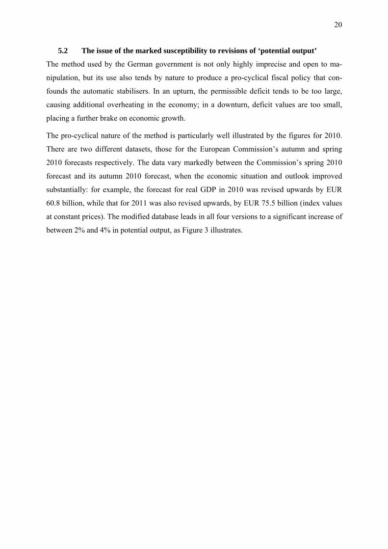
5.2 The issue of the marked susceptibility to revisions of ‘potential output’

The method used by the German government is not only highly imprecise and open to ma-

nipulation, but its use also tends by nature to produce a pro-cyclical fiscal policy that con-

founds the automatic stabilisers. In an upturn, the permissible deficit tends to be too large,

causing additional overheating in the economy; in a downturn, deficit values are too small,

placing a further brake on economic growth.

The pro-cyclical nature of the method is particularly well illustrated by the figures for 2010.

There are two different datasets, those for the European Commission’s autumn and spring

2010 forecasts respectively. The data vary markedly between the Commission’s spring 2010

forecast and its autumn 2010 forecast, when the economic situation and outlook improved

substantially: for example, the forecast for real GDP in 2010 was revised upwards by EUR

60.8 billion, while that for 2011 was also revised upwards, by EUR 75.5 billion (index values

at constant prices). The modified database leads in all four versions to a significant increase of

between 2% and 4% in potential output, as Figure 3 illustrates.

 

21

Figure 3: Amended output potential as a result of a change of data against the background of a constant

specification

Source: EU Commission, authors’ own calculations

 

22

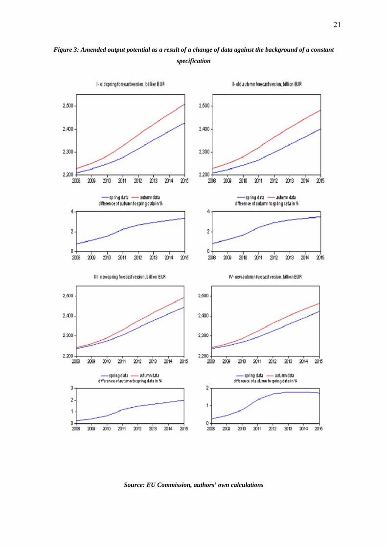
Table 4: Pro-cyclical revision and weakening of the automatic stabilisers

Source: EU Commission, authors’ own calculations

Depending on the method, this has substantial and quantifiable impact on the estimate for

nominal GDP and output potential. The method that is least dependent on cyclical factors is

the spring version of the new method: in this version, the EUR 46.9 billion increase in the

GDP forecast in 2010 and the EUR 73.1 billion increase for 2011 produce changes in the es-

timated potential of EUR -5 billion and EUR 18 billion respectively. The autumn version of

the old method is, by contrast, the one most dependent on cyclical factors: EUR 20.5 billion

and EUR 49.7 billion respectively – that is, more than 50% and more than 70% of the in-

crease in GDP respectively – are added to potential, meaning that potential itself rises mark-

edly because the economy is doing better.

The extent to which potential is reliant on cyclical factors is, however, not merely an aca-

demic detail but is of direct practical relevance for Germany’s budget policy in the context of

the debt brake: on the basis of the new potential values, and in combination with the new

GDP values, output gap values must be recalculated which, when multiplied by the relevant

budget sensitivity figure (0.248 in 2010 and 0.16 in 2011), produce a further change in the

cyclical components. This change ranges from EUR 6.6 billion (2010) to EUR 3.7 billion

(2011) in the autumn version of the old method and from EUR 12.9 billion (2010) to EUR 8.8

billion (2011) in the spring version of the new method. Hence, the forecast economic upturn

produces radically different reductions in the permitted cyclical deficit, depending on the ver-

sion used.

 

23

The cyclically determined figure for budget consolidation derived in this way does not, how-

ever, equate with the actual cyclically determined impact of the higher growth forecast on

public budgets, which depends directly on the forecast growth in actual GDP against constant

potential and is, therefore, markedly higher. In a period of economic recovery, this results in

the cyclically determined budget consolidation varying according to the method and version

used; fiscal policy prevents the automatic stabilisers from having their full effect and, for this

reason, is too expansive in pro-cyclical terms or conversely, in a downturn, produces an ex-

cessively contractionary pro-cyclical effect.

In the simulations we have carried out, the effect is of a very relevant magnitude. In the case

of the pro-cyclical autumn version of the old method, the Bund would have excessive margins

for 2010 and 2011 of EUR 17 billion, while in the case of the least pro-cyclical spring version

of the new method, the margins would still be just under EUR 7.5 billion. This picture is re-

versed in the case of a downturn: in such a situation, the budget would have too little eco-

nomic room for manoeuvre and this would pro-cyclically strengthen the downturn, with the

automatic stabilisers weakened by between 15% and 70%, depending on the version.

5.3 Simulating a future economic downturn6

The issue of the impact of such a debt brake on the future of federal budget policy becomes

particularly significant in the event that Germany undergoes another period of weak economic

growth, which is currently far from unlikely. To the best of the authors’ knowledge, there are

no ex-ante simulations of the impact such a scenario would have within the framework of a

debt brake. The only simulations there have been are at European level and have been carried

out in conjunction with simulations of the issue of estimating potential output (D’Auria 2010).

It is incomprehensible that such research has been neglected in Germany when a constitu-

tional rule is being introduced. From an economic perspective, it is particularly vital during a

period of economic crisis that the automatic stabilisers can function appropriately, not least

because it is otherwise impossible to take discretionary measures without invoking the ‘ex-

ception clause’.

The structural deficit for 2011 is currently markedly below the maximum permissible deficit

under the government’s deficit reduction course, but, as we have shown, this can be attributed

to two main factors. First, the German government has so far benefited from favourable eco-

nomic trends arising from the pro-cyclical bias in the cyclical adjustment process. Second, the

initial deficit set out in the deficit reduction plan in spring 2010 was determined on the basis

6 The following analysis is based on calculations carried out as part of the IMK’s estimate of tax revenues in May 2011: Truger et al (2011).

 

24

of a modest economic outlook and the old TFP method, which was very high at 2.2% (the ‘ski

jump effect’). Since then, the German government has not needed to make use of the credit

line available to it and, in fact, the resulting margins have widened consistently. Were there to

be a further economic downturn, however, these positive trends could easily be reversed, as

the simulation demonstrates.

The simulation can be divided into various stages. First, the macroeconomic framework for a

further downturn (IMK risk scenario) compared to a reference scenario (IMK basic scenario)

was established, followed by a fiscal estimate, producing a required net borrowing value for

the country’s medium-term budgetary planning against a backdrop of otherwise identical ex-

penditure and revenue conditions. Then the cyclical components according to the debt brake

procedure were calculated dynamically, using the changing supporting periods, so that the

cyclical elements could be deducted from the total deficit.

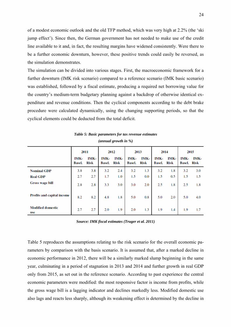
Table 5: Basic parameters for tax revenue estimates

(annual growth in %)

Source: IMK fiscal estimates (Truger et al. 2011)

Table 5 reproduces the assumptions relating to the risk scenario for the overall economic pa-

rameters by comparison with the basis scenario. It is assumed that, after a marked decline in

economic performance in 2012, there will be a similarly marked slump beginning in the same

year, culminating in a period of stagnation in 2013 and 2014 and further growth in real GDP

only from 2015, as set out in the reference scenario. According to past experience the central

economic parameters were modified: the most responsive factor is income from profits, while

the gross wage bill is a lagging indicator and declines markedly less. Modified domestic use

also lags and reacts less sharply, although its weakening effect is determined by the decline in

 

25

consumer spending. By contrast, it is assumed that government spending and public invest-

ment are not adjusted – an optimistic assumption, given past experience.

Table 6 reproduces the fiscal revenue estimates generated by the BMF and the IMK basic and

risk scenarios. In the interests of simplification, the risk scenario provides details of only the

most important taxes shared by all levels of government (tax on personal and corporate in-

come, value added tax) and business tax: in the case of purely federal taxes (mostly indirect

taxes) and local tax (excluding business tax) a 0.5 elasticity compared with nominal GDP has

been assumed. Import duty figures assume a slight fall on the basis of an expected fall in im-

ports.

Table 6: Outcome of tax revenue estimates for the Federal level in EUR billion

Source: Working Group on Tax Estimates; IMK tax revenue estimates

As expected, this produces a significant drop in revenue for the Bund by comparison with the

basic scenario. In the first year of lower economic growth – 2012 – the drop in revenue is

relatively modest, at EUR 3.3 billion, but then, as a result of a severe slump in the economy, it

rises rapidly to EUR 13.5 billion in 2014 and EUR 17.0 billion in 2015. By 2015, the cumula-

tive loss of revenue compared with the basic scenario totals EUR 42.6 billion. This would

dramatically worsen prospects for the Bund.

The basic parameters used by the German government to draw up the country’s budget and

finance trends to 2015 and the calculations for debt brake targets produce an annual margin of

about EUR 10 billion for the period from 2012 to 2014. On the basis of an assumed rise in

expenditure and as yet inadequately quantified budget-balancing measures, the margin in

2015 falls to just under EUR 9 billion (Figure 4). It is important to stress that the resulting

margins have not been ‘created’ by, for example, particular additional discretionary budget

consolidation measures by the government but, as already indicated, are the result particularly

 

26

of an upturn in the economy and the legitimate exploitation of the scope for manipulation –

the ‘ski jump effect’ and the change of method for calculating TFP. The resulting margins

have led to radically differing proposals for fiscal policy. In some cases, there have been calls

for additional tax cuts, while the opposition SPD in the Bundestag, the German Federal Audit

Office (Bundesrechnungshof), and the Bundesbank have all called for the margins to be

scrapped by means of a retrospective recalculation of the basic deficit and/or for the govern-

ment to revert to the old EU method.

A different recommendation would be to use the margins as a buffer against the possible

threat of a medium-term economic downturn. The justification for this can be illustrated per-

fectly by using the impact on the federal budget of the assumed risk scenario: this needs to

take into account not only of the effects on the country’s tax revenues of the assumed weaken-

ing in economic growth outlined above but also of the complex repercussions of economic

development on the permissible deficits under the debt brake.

In order to include these effects, we adopted the following methodology. First, basic scenario

calculations were made for output potential, output gap and cyclical components for the years

2012 to 2015, based as closely as possible on published BMF data.7 Then, using the same

method, we made the same calculations for the risk scenario. This assumes that when it draws

up its budget, the German government knows the likely economic trends for the year for

which it is drawing up a budget and for the following year, in accordance with the rules set

out in the risk scenario. The result is that the economic outlook worsens steadily compared

with the basic scenario and the estimates for potential output, the output gap and cyclical

components are adjusted year by year. For the purposes of simplification, we have excluded

possible forecasting errors and, hence, necessary posting to the control account.

7 The BMF publishes only time series, which do not enable meaningful conclusions to be drawn about the specifi-cations. It is also unclear which values were generated during the estimating process and which were exogenous and added subsequently. The series published since the spring of 2011 represent progress compared with the BMF’s approach in 2009 and 2010, when not even data series were published. It is unclear, however, why the BMF persists in refusing to publish the data and specifications on which its forecasts are based, as the European Commission does, and so make it possible to scrutinise its forecasts rigorously.

 

27

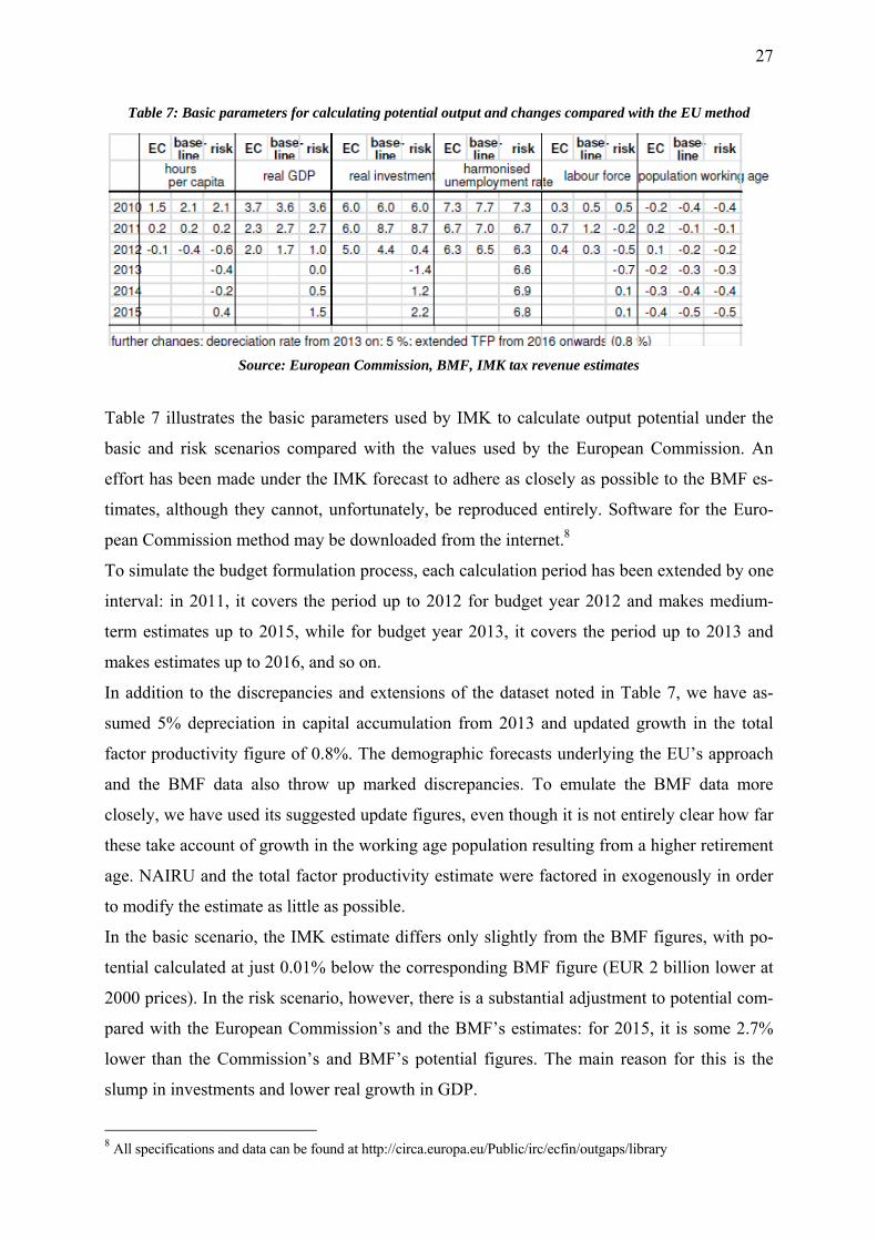
Table 7: Basic parameters for calculating potential output and changes compared with the EU method

Source: European Commission, BMF, IMK tax revenue estimates

Table 7 illustrates the basic parameters used by IMK to calculate output potential under the

basic and risk scenarios compared with the values used by the European Commission. An

effort has been made under the IMK forecast to adhere as closely as possible to the BMF es-

timates, although they cannot, unfortunately, be reproduced entirely. Software for the Euro-

pean Commission method may be downloaded from the internet.8

To simulate the budget formulation process, each calculation period has been extended by one

interval: in 2011, it covers the period up to 2012 for budget year 2012 and makes medium-

term estimates up to 2015, while for budget year 2013, it covers the period up to 2013 and

makes estimates up to 2016, and so on.

In addition to the discrepancies and extensions of the dataset noted in Table 7, we have as-

sumed 5% depreciation in capital accumulation from 2013 and updated growth in the total

factor productivity figure of 0.8%. The demographic forecasts underlying the EU’s approach

and the BMF data also throw up marked discrepancies. To emulate the BMF data more

closely, we have used its suggested update figures, even though it is not entirely clear how far

these take account of growth in the working age population resulting from a higher retirement

age. NAIRU and the total factor productivity estimate were factored in exogenously in order

to modify the estimate as little as possible.

In the basic scenario, the IMK estimate differs only slightly from the BMF figures, with po-

tential calculated at just 0.01% below the corresponding BMF figure (EUR 2 billion lower at

2000 prices). In the risk scenario, however, there is a substantial adjustment to potential com-

pared with the European Commission’s and the BMF’s estimates: for 2015, it is some 2.7%

lower than the Commission’s and BMF’s potential figures. The main reason for this is the

slump in investments and lower real growth in GDP.

8 All specifications and data can be found at http://circa.europa.eu/Public/irc/ecfin/outgaps/library

 

28

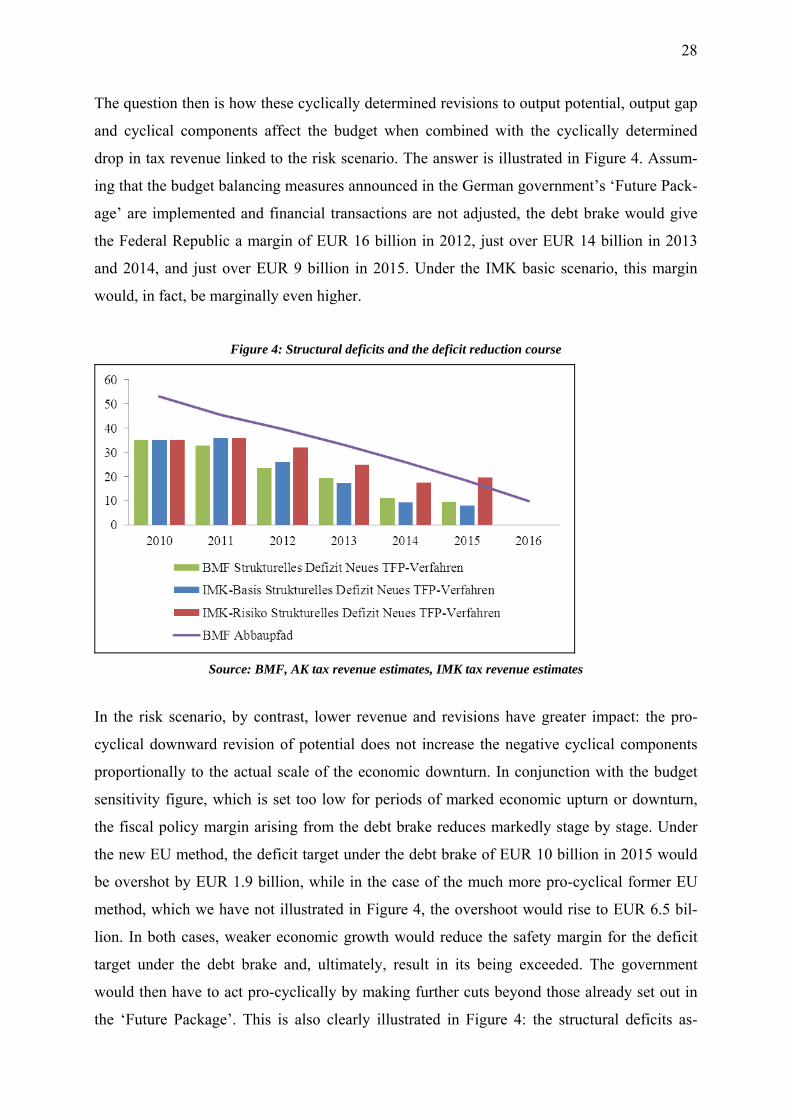
The question then is how these cyclically determined revisions to output potential, output gap

and cyclical components affect the budget when combined with the cyclically determined

drop in tax revenue linked to the risk scenario. The answer is illustrated in Figure 4. Assum-

ing that the budget balancing measures announced in the German government’s ‘Future Pack-

age’ are implemented and financial transactions are not adjusted, the debt brake would give

the Federal Republic a margin of EUR 16 billion in 2012, just over EUR 14 billion in 2013

and 2014, and just over EUR 9 billion in 2015. Under the IMK basic scenario, this margin

would, in fact, be marginally even higher.

Figure 4: Structural deficits and the deficit reduction course

Source: BMF, AK tax revenue estimates, IMK tax revenue estimates

In the risk scenario, by contrast, lower revenue and revisions have greater impact: the pro-

cyclical downward revision of potential does not increase the negative cyclical components

proportionally to the actual scale of the economic downturn. In conjunction with the budget

sensitivity figure, which is set too low for periods of marked economic upturn or downturn,

the fiscal policy margin arising from the debt brake reduces markedly stage by stage. Under

the new EU method, the deficit target under the debt brake of EUR 10 billion in 2015 would

be overshot by EUR 1.9 billion, while in the case of the much more pro-cyclical former EU

method, which we have not illustrated in Figure 4, the overshoot would rise to EUR 6.5 bil-

lion. In both cases, weaker economic growth would reduce the safety margin for the deficit

target under the debt brake and, ultimately, result in its being exceeded. The government

would then have to act pro-cyclically by making further cuts beyond those already set out in

the ‘Future Package’. This is also clearly illustrated in Figure 4: the structural deficits as-

 

29

sumed in the IMK risk scenario for 2015 (here, the new TFP method) exceed the deficit re-

duction course targets. If there were also to be tax cuts – as looks increasingly likely from

2013 – then the discretionary adjustments and cuts would have to be correspondingly greater.

Given the gathering economic gloom, that would be a serious mistake. The fact that the most

recent tax revenue estimate (November 2011) assumes a modest increase in revenue for the

medium term (2013 and beyond) is based on the assumption of prompt economic recovery in

2013. Were this not to materialise, or if the downturn in the following year were to be more

marked than assumed, then revenue would rapidly drop.

6. Conclusions

This paper has considered in concrete terms the effect of the German government’s detailed

debt brake, to show that the method chosen for calculating the structural deficit is extremely

complex and, for that reason alone, highly opaque and open to manipulation. The German

government has actually exacerbated the resulting lack of transparency by failing to provide

proper information and has used the existing scope for intervention in a technically adroit way

to broaden its margins in budgetary terms. Its satisfaction with this outcome may, however, be

short-lived, because on the basis of the pro-cyclical approach stipulated in the technical pro-

cedure, the margins would rapidly disappear again if there were to be a major economic

downturn – and this would be a certainty if combined with further tax cuts. In the worst case,

Germany’s fiscal policy would then become even more restrictive right in the midst of a

Europe-wide economic crisis. Ingolf Deubel, former Finance Minister of the Rhineland-

Palatinate and one of the founding fathers of the debt brake in the Second Federalism Reform

Commission, has now conceded that, although he is

“a trained public finance economist and econometrician, I […] did not have a com-

plete overview of the consequences of this implementing legislation for the German

government’s budget when I voted for it in the Bundesrat. […] Knowing what I know

today, I would now strongly counsel the government against defining such a vague

process so precisely and restrictively.” Deubel (2010, p.2).

There is not much one can add to that argument. It is less than clear how a rule of this kind

governing deficits and the German government’s initial concrete application of it will seri-

ously boost the confidence of the financial markets in Germany’s fiscal policy. Those who,

nonetheless, justify a debt brake by citing such beneficial effects must either be assuming that

 

30

the financial markets are economically irrational or themselves be using arguments that lack

an economic rationale.

References

Anderson, B., Minarik, J.J. (2006): Design Choices for Fiscal Policy Rules, OECD journal on budgeting, vol. 5, no. 4, 2006, pp.159-208.

Bruchez, P.-A. (2003): A Modification of the HP Filter Aiming at Reducing the End-Point Bias, Swiss Financial Administration, Working Paper ÖT/2003/3, Bern.

Caner, M., Grennes, T., Koehler-Geib, F. (2011): Finding the Tipping-Point – When Sovereign Debt Turns bad, World Bank Policy Research Paper 5391.

Cecchetti, S.G., Mohanty, M.S., Zampolli, F. (2011): The real effects of debt, BIS Working Paper.

Checherita, C., Rother, P. (2010): The Impact of High and Growing Debt on Economic Growth. An Empirical Investigation for the Euro Area, ECB Working Paper no. 1237, Frankfurt.

D’Auria, F., Denis, C., Havik, K., McMorrow, K., Planas, C., Raciborski, R., Röger, R., Rossi, A. (2010): The Production Function Methodology for Calculating Potential Growth Rates and Output Gaps. European Commission, Economic Papers 420, Brussels.

Deubel, I. (2010): Konjunkturausregulierung und Länderhaushalte. Ein Beitrag zur prakti-schen Umsetzung der Schuldenbremse und des Konsolidierungshilfengesetzes, Bad Kreuznach.

Deutsche Bundesbank, Anforderungen an die Konjunkturbereinigung im Rahmen der neuen Schuldenregel, Januar 2011, monthly report, pp.59-64.

GD [Projektgruppe Gemeinschaftsdiagnose: project group joint forecast] (2010): Herbstgutachten. Deutschland im Aufschwung. Wirtschaftspolitik vor wichtigen Entscheidungen, Munich.

GD [Projektgruppe Gemeinschaftsdiagnose: project group joint forecast] (2011): Herbstgutach-ten. Europäische Schuldenkrise belastet deutsche Konjunktur, Munich, 2011.

Girouard, N., André, C. (2005): Measuring Cyclically-Adjusted Budget Balances for OECD Countries, OECD Working Paper no. 434, Paris.

Heinemann, F., Moessinger, M.-D., Osterloh, S. (2011): Nationale Fiskalregeln – Ein Instrument zur Vorbeugung von Vertrauenskrisen? Summary of a research study by the Cen-tre for Economic Research, Mannheim; August 2011 monthly report of the Germany Minis-try of Finance (BMF), pp.58-66.

Horn, G., Logeay, C., Tober, S. (2007): Estimating Germany’s Potential Output, IMK Work-ing Paper no. 2/2007, Duesseldorf.

Horn, G., Niechoj, T. Proaño, C., Truger, A., Vesper, D., Zwiener, R. (2008): Die Schulden-bremse – eine Wachstumsbremse? IMK Report no. 29, 2008.

Horn, G., Truger, A., Proaño, C. (2009): IMK Policy Brief, 2009.

Horn, G., Tober, S., van Treeck,T., Truger, A. (2010a): Euroraum vor der Zerreißprobe? IMK Report, Nr. 48.

 

31

Horn, A., Niechoj, T., Tober, S., van Treeck, T., Truger, A. (2010b): Reform des Stabilitäts- und Wachstumspakts: Nicht nur öffentliche, auch private Verschuldung zählt. IMK Report, Nr. 51, Juli 2010.

Horn, G., Lindner, F., Niechoj, T., Sturn, S., Tober, S., Truger, A., Will, H. (2011a): Herausforderungen für die Wirtschaftspolitik 2011. IMK Report, no. 59, 2011.

Horn, G., Lindner, F., Niechoj, T. (2011b): Schuldenschnitt für Griechenland - ein gefährli-cher Irrweg für den Euroraum. IMK Report, Nr. 63.

Horn, G., Lindner, F., Niechoj, T., Truger, A., Will, H. (2011c): Voraussetzungen einer er-folgreichen Konsolidierung Griechenlands, IMK Report, Nr. 66.

IMF [International Monetary Fund] (2011): Modernizing the Framework for Fiscal Policy and Public Debt Sustainability Analysis, IMF Policy Papers, Washington.

IMK, OFCE, WIFO, Der Euroraum im Umbruch. Erste gemeinsame Diagnose des Makro-Konsortiums. IMK Report, no. 61, April 2011.

Kopits, G., Symansky, S. (1998): Fiscal Policy Rules, IMF Occasional Paper no. 162, Wash-ington.

Kumar, M.S., Woo, J. (2010): Public Debt and Growth, IMF Working Paper no. 10/174, Wash-ington.

Musgrave, R.A. (1959): The Theory of Public Finance. A Study in Public Economy, New York et al.: McGraw-Hill.

Ostry, J.D., Ghosh, A.R., Kim, J.I., Qureshi, M.S. (2010): Fiscal Space, IMF Staff Position Note 10/11, Washington.

Reinhardt, C.M., Rogoff, K.S. (2010): Growth in a Time of Debt, NBER Working Paper no. 15639, Washington.

SVR [Sachverständigenrat zur Begutachtung der gesamtwirtschaftlichen Entwicklung, Ger-man Council of Economic Experts] (2007): Staatsverschuldung wirksam begrenzen. Study on behalf of the Federal Minister for Economics and Technology, Wiesbaden.

SVR (2010): Chancen für einen stabilen Aufschwung. Annual report 2010/2011, Wiesbaden.

Truger, A. (2004): Rot-grüne Steuerreformen, Finanzpolitik und makroökonomische Perfor-mance – was ist schief gelaufen?, in: Hein, E., Heise, A. und Truger, A. (eds.): Finanzpoli-tik in der Kontroverse, Marburg (Metropolis), pp.169-208.

Truger, A. (2009): Ökonomische und soziale Kosten von Steuersenkungen. Prokla 154 (1/2009), pp.27-46.

Truger, A. (2010): Schwerer Rückfall in alte Obsessionen – Zur aktuellen deutschen Finanzpo-litik, Intervention. European Journal of Economics and Economic Policies 1/2010, pp.11-24.

Truger, A., Teichmann, D. (2011): Zur Reform des Einkommensteuertarifs. Ein Reader der Parlamentarischen Linken in der SPD-Bundestagsfraktion, Berlin / Düsseldorf.

 

32

Truger, A., Will, H. (2009): Finanzpolitische und makroökonomische Risiken der Schulden-bremse in Schleswig-Holstein. Evidence given by the Hans Böckler Foundation’s Macro-economic Policy Institute (IMK) during written consultation carried out by the Home and Legal Affairs Committee of the regional parliament for Schleswig-Holstein on the motion from the CDU and SPD groups on “Balancing the budget; cutting new borrowing to zero” (publication 16/2771, para. 4), IMK Policy Brief.

Truger, A., Will, H., Köhrsen, J. (2009): Die Schuldenbremse: Eine schwere Bürde für die Finanzpolitik. Evidence given by the Hans Böckler Foundation’s Macroeconomic Policy Institute (IMK) during the public consultation carried out by the regional parliament for North Rhine Westphalia on 17 September 2009, IMK Policy Brief, 2009.

Truger, A., Will, H., Teichmann, D. (2011): IMK Steuerschätzung 2011-2015. Kräftige Mehreinnahmen: kein Grund für finanzpolitischen Übermut, IMK Report no. 62, 2011.