Embed Size (px)
Citation preview
Open Research OnlineThe Open University’s repository of research publicationsand other research outputs
The 2dF-SDSS LRG and QSO Survey: thespectroscopic QSO catalogueJournal ItemHow to cite:
Croom, Scott M.; Richards, Gordon T.; Shanks, Tom; Boyle, Brian J.; Sharp, Robert G.; Bland-Hawthorn,Joss; Bridges, Terry; Brunner, Robert J.; Cannon, Russell; Carson, Daniel; Chiu, Kuenley; Colless, Matthew; Couch,Warrick; De Propris, Roberto; Drinkwater, Michael J.; Edge, Alastair; Fine, Stephen; Loveday, Jon; Miller, Lance;Myers, Adam D.; Nichol, Robert C.; Outram, Phil; Pimbblet, Kevin; Roseboom, Isaac; Ross, Nicholas; Schneider,Donald P.; Smith, Allyn; Stoughton, Chris; Strauss, Michael A. and Wake, David (2009). The 2dF-SDSS LRG andQSO Survey: the spectroscopic QSO catalogue. Monthly Notices of the Royal Astronomical Society, 392(1) pp.19–44.
For guidance on citations see FAQs.
c© 2008 The Authors
Version: Version of Record
Link(s) to article on publisher’s website:http://dx.doi.org/10.1111/j.1365-2966.2008.14052.x
Copyright and Moral Rights for the articles on this site are retained by the individual authors and/or other copyrightowners. For more information on Open Research Online’s data policy on reuse of materials please consult the policiespage.
oro.open.ac.uk
Mon. Not. R. Astron. Soc. 392, 19–44 (2009) doi:10.1111/j.1365-2966.2008.14052.x
The 2dF-SDSS LRG and QSO Survey: the spectroscopic QSO catalogue
Scott M. Croom,1,2� Gordon T. Richards,3 Tom Shanks,4 Brian J. Boyle,5
Robert G. Sharp,2 Joss Bland-Hawthorn,1,2 Terry Bridges,2 Robert J. Brunner,6
Russell Cannon,2 Daniel Carson,7 Kuenley Chiu,8 Matthew Colless,2 Warrick Couch,9
Roberto De Propris,10 Michael J. Drinkwater,11 Alastair Edge,4 Stephen Fine,1
Jon Loveday,12 Lance Miller,13 Adam D. Myers,6 Robert C. Nichol,7 Phil Outram,4
Kevin Pimbblet,11 Isaac Roseboom,11,12 Nicholas Ross,4,14 Donald P. Schneider,14
Allyn Smith,15 Chris Stoughton,16 Michael A. Strauss17 and David Wake4
1Institute of Astronomy, School of Physics, University of Sydney, NSW 2006, Australia2Anglo-Australian Observatory, PO Box 296, Epping, NSW 1710, Australia3Department of Physics, Drexel University, Philadelphia, PA 19104, USA4Department of Physics, University of Durham, South Road, Durham DH1 3LE5Australia Telescope National Facility, PO Box 76, Epping, NSW 1710, Australia6Department of Astronomy, University of Illinois at Urbana-Champaign, Urbana, IL 61801, USA7Institute of Cosmology and Gravitation, Mercantile House, Hampshire Terrace, University of Portsmouth, Portsmouth PO1 2EG8School of Physics, University of Exeter, Stocker Road, Exeter EX4 4QL9Centre for Astrophysics & Supercomputing, Swinburne University of Technology, PO Box 218, Hawthorn, VIC 3122, Australia10Cerro Tololo Inter-American Observatory, Casilla 603, La Serena, Chile11Department of Physics, University of Queensland, Brisbane, QLD 4072, Australia12Astronomy Centre, University of Sussex, Falmer, Brighton BN1 9QJ13Department of Physics, Oxford University, 1 Keble Road, Oxford OX1 3RH14Department of Astronomy and Astrophysics, 525 Davey Laboratory, Pennsylvania State University, University Park, PA 16802, USA15Department of Physics and Astronomy, University of Wyoming, PO Box 3905, Laramie, WY 82071, USA16Fermi National Accelerator Laboratory, PO Box 500, Batavia, IL 60510, USA17Princeton University Observatory, Peyton Hall, Princeton, NJ 08544, USA
Accepted 2008 October 1. Received 2008 October 1; in original form 2008 July 29
ABSTRACT
We present the final spectroscopic QSO catalogue from the 2dF-SDSS LRG (luminous redgalaxy) and QSO (2SLAQ) survey. This is a deep, 18 < g < 21.85 (extinction corrected),sample aimed at probing in detail the faint end of the broad line active galactic nuclei luminositydistribution at z � 2.6. The candidate QSOs were selected from SDSS photometry and observedspectroscopically with the 2dF spectrograph on the Anglo-Australian Telescope. This samplecovers an area of 191.9 deg2 and contains new spectra of 16 326 objects, of which 8764 areQSOs and 7623 are newly discovered [the remainder were previously identified by the 2dFQSO Redshift Survey (2QZ) and SDSS]. The full QSO sample (including objects previouslyobserved in the SDSS and 2QZ surveys) contains 12 702 QSOs. The new 2SLAQ spectroscopicdata set also contains 2343 Galactic stars, including 362 white dwarfs, and 2924 narrowemission-line galaxies with a median redshift of z = 0.22.
We present detailed completeness estimates for the survey, based on modelling of QSOcolours, including host-galaxy contributions. This calculation shows that at g � 21.85 QSOcolours are significantly affected by the presence of a host galaxy up to redshift z ∼ 1 in theSDSS ugriz bands. In particular, we see a significant reddening of the objects in g − i towardsthe fainter g-band magnitudes. This reddening is consistent with the QSO host galaxies beingdominated by a stellar population of age at least 2–3 Gyr.
�E-mail: [email protected]
C© 2008 The Authors. Journal compilation C© 2008 RAS
at Oxford Journals on Septem
ber 19, 2013http://m
nras.oxfordjournals.org/D
ownloaded from

20 S. M. Croom et al.
The full catalogue, including completeness estimates, is available on-line athttp://www.2slaq.info/.
Key words: catalogues – surveys – white dwarfs – galaxies: active – quasars: general –galaxies: Seyfert.
1 IN T RO D U C T I O N
The last decade has seen the coming of age of extremely high mul-tiplex fibre spectroscopy, as implemented by the 2-degree Field(2dF) instrument (Lewis et al. 2002) and the Sloan Digital SkySurvey (SDSS; York et al. 2000). These new facilities have al-lowed order of magnitude increases in sample sizes over the previ-ous generation of surveys. The 2dF QSO Redshift Survey (2QZ;Croom et al. 2001a, 2004, hereafter C04) and the SDSS QSOsurvey (Schneider et al. 2007) have allowed precise measurementof the evolution of QSOs (e.g. Boyle et al. 2000; C04; Richardset al. 2006), QSO clustering (e.g. Croom et al. 2001b, 2005;Shen et al. 2007), spectral properties (e.g. Vanden Berk et al. 2001;Croom et al. 2002; Richards et al. 2002a; Corbett et al. 2003) anda range of other significant results. The published sample sizes(∼25 000 QSOs in 2QZ; ∼80 000 QSOs in SDSS) are large enoughthat in many cases measurements are now limited by systematicuncertainties rather than random errors.
However, one of the important limitations of the 2QZ and SDSSsurveys are their relative depths. The SDSS QSO survey is limitedto i = 19.1, or i = 20.2 for the high-redshift sample (Richardset al. 2002b), which does not reach the break in the QSO lumi-nosity function (LF). 2QZ is somewhat deeper, limited in the bluerbJ band to bJ < 20.85. The 2QZ clearly shows the break in theQSO LF, typically reaching ∼1 mag fainter than the break at z < 2.The observed break in the LF is a gradual flattening towards faintmagnitudes; as a result the constraints from the 2QZ on the ac-tual slope of the faint end are fairly uncertain, as evidenced by thedifference between the results from the first release (Boyle et al.2000) and the final release (C04). In comparison, X-ray surveys,in particular, using Chandra (e.g. Giacconi et al. 2002; Alexan-der et al. 2003) and XMM–Newton (e.g. Hasinger et al. 2001;Worsley et al. 2004; Barcons et al. 2007), reach to fainter depths,but over a much smaller area. The largest samples contain ∼1000objects over a few square degrees. These surveys have demonstratedthat the pure luminosity evolution that appears to model theevolution of the most extensive optical samples (e.g. 2QZ, SDSS)fails to trace the evolution of the faint active galactic nuclei (AGN)populations at L < L∗. It now appears that the activity in faintAGN peaks at a lower redshift than that of more luminous AGN(e.g. Hasinger, Miyaji & Schmidt 2005); this process has been de-scribed as AGN downsizing (e.g. Barger et al. 2005). Whether thedownsizing is due to lower mass black holes (BHs) being moreactive at low redshift (e.g. Heckman et al. 2004) or massive BHsat lower rates of accretion (e.g. Babic et al. 2007) remains unclear.Both effects are likely to play a role.
Substantial advances have been made in the theoretical under-standing of AGN formation and the connection to galaxy formation(e.g. Hopkins et al. 2005a). This work has largely been driven bythe observational evidence that most massive galaxies with bulgescontain supermassive BHs (SMBHs) (e.g. Tremaine et al. 2002).SMBH accretion is thought to be triggered (at least for moderate
to high-luminosity AGN) by the merger of gas-rich galaxies; whilethe time-scale for the merger may be as long as ∼1 Gyr, duringthe majority of this time the accretion is obscured from view. It isonly when the AGN finally expels the surrounding gas and dustthat it shines like a quasar for a brief period (∼100 Myr), beforeexhausting its fuel supply (e.g. Di Matteo, Springel & Hernquist2005). This feedback of the AGN into the host also heats (and pos-sibly expels) the gas in the galaxy, which suppresses star formationleading to ‘red and dead’ ellipticals or bulges. These models matcha number of previous observations and predict that the faint endof the QSO LF is largely composed of higher mass BHs at loweraccretion rates (i.e. below their peak luminosity; Hopkins et al.2005b).
The 2dF SDSS LRG (luminous red galaxy) and QSO (2SLAQ)survey was designed to survey optically faint AGN/QSOs within asufficiently large volume to obtain robust measurements of both theLF and QSO clustering. Throughout this paper, we will use the termQSO to refer to any broad line (type 1) AGN, irrespective of lumi-nosity. The QSO portion of the survey shared fibres with a relatedprogramme to target LRGs at z � 0.4–0.7 (Cannon et al. 2006). Boththe LRGs and QSOs were selected from single epoch SDSS imagingdata, and then observed spectroscopically with the 2dF instrumentat the Anglo-Australian Telescope (AAT). The 2SLAQ QSO samplehas already produced a preliminary QSO LF (Richards et al. 2005;hereafter R05), measured the clustering of QSOs as a function ofluminosity (da Angela et al. 2008) and studied the distribution ofQSO broad line widths (Fine et al. 2008). In this paper, we presentthe final spectroscopic QSO catalogue of the 2SLAQ sample. Wethen carry out a detailed analysis of the survey completeness. Theanalysis of the QSO LF from the final 2SLAQ sample is presentedin a companion paper (Croom et al., in preparation).
In Section 2, we discuss the selection of QSO candidates fromthe SDSS imaging data. This has largely been described by R05,but is summarized here for completeness. In Section 3, we presentthe spectroscopic observations, and in Section 4, we describe thecomposition and quality of the resulting catalogue. Section 5 con-tains our detailed completeness analysis. We summarize our resultsin Section 6. Throughout this paper, we will assume a cosmologywith H0 = 70 km s−1 Mpc−1, �m = 0.3 and �� = 0.7.
2 IM AG I N G DATA A N D Q S O SE L E C T I O N
2.1 The SDSS imaging data
The photometric measurements used as the basis for our catalogueare drawn from the Data Release 1 (DR1) processing (Stoughtonet al. 2002; Abazajian et al. 2003) of the SDSS imaging data. Theastrometric precision at the faint limit of the survey is ∼0.1 arcsec(Pier et al. 2003). The SDSS data are taken in five photometricpassbands (ugriz; Fukugita et al. 1996) using a large format CCDcamera (Gunn et al. 1998) on a special-purpose 2.5-m telescope(Gunn et al. 2006). The regions covered by the 2SLAQ survey were
C© 2008 The Authors. Journal compilation C© 2008 RAS, MNRAS 392, 19–44
at Oxford Journals on Septem
ber 19, 2013http://m
nras.oxfordjournals.org/D
ownloaded from
The 2SLAQ QSO catalogue 21
complete in DR1, so no further updates to more recent data releasesare required. Except where otherwise stated, all SDSS magnitudesdiscussed herein are ‘asinh’ point spread function (PSF) magnitudes(Lupton, Gunn & Szalay 1999) on the SDSS pseudo-AB magnitudesystem (Oke & Gunn 1983) that have been dereddened for Galacticextinction according to the model of Schlegel, Finkbeiner & Davis(1998). The SDSS Quasar Survey (Schneider et al. 2007) extends toi = 19.1 for z < 3 and i = 20.2 for z > 3; our work herein exploresthe z < 3 regime to g = 21.85 (i ∼ 21.63, based on the mediancolours of SDSS QSOs; e.g. Richards et al. 2001). At the faint limitof the 2SLAQ sample (21.75 < g < 21.85), the photometric errorsare typically �u = 0.20, �g = 0.07, �r = 0.08, �i = 0.11 and�z = 0.33.
2.2 Sample selection
2.2.1 Preliminary sample restrictions
Our quasar candidate sample was drawn from 10 SDSS imagingruns. Because of the slightly poorer image quality in the sixth rowof CCDs in the SDSS camera we did not include these data. Thusthe 2SLAQ survey regions are 2◦ wide rather than the usual 2.◦5 foran SDSS imaging run. We rejected any objects that met the ‘fatal’or ‘non-fatal’ error definitions of the SDSS quasar target selection(Richards et al. 2002a). Although our survey covers the southernequatorial Stripe 82 region which has been scanned multiple times(Adelman-McCarthy et al. 2008), the co-added data (Annis et al.2006) were not available at the time of our spectroscopic observa-tions and so single scan data were used.
We apply a limit to the (extinction corrected) i-band PSF mag-nitude of i < 22.0 and σi < 0.2. We also placed restrictions on theerrors in each of the other four bands: σu < 0.4, σg < 0.13, σr <
0.13 and σz < 0.6. Note that this selection of error constraints effec-tively limits the redshift to less than 3, as the Lyα forest suppressesthe u flux at higher redshifts.
2.2.2 Low-redshift colour cuts
Based on spectroscopic identifications (IDs) from SDSS and 2QZ ofthis initial set of objects, we implement additional colour cuts thatare designed to select faint ultraviolet-excess (UVX) QSOs withhigh efficiency and completeness at redshifts z � 2.6. An analysisof the completeness of the selection algorithm is given as a functionof redshift and magnitude in Section 5.2.
We reject hot white dwarfs using the following cuts, independentof magnitude. Specifically, we rejected objects that satisfy the con-dition: A AND [(B AND C AND D) OR E], where the letters referto the cuts:
A) −1.0 < u − g < 0.8
B) −0.8 < g − r < 0.0
C) −0.6 < r − i < −0.1
D) −1.0 < i − z < −0.1
E) −1.5 < g − i < −0.3.
(1)
These constraints are similar to the white dwarf cut applied byRichards et al. (2002a, their equation 2) except for the added cutwith respect to the g − i colour.
To efficiently target both bright and faint targets, we use differentcolour cuts as a function of g-band magnitude. The bright sample isrestricted to 18.0 < g < 21.15 and is designed to allow for overlapwith previous SDSS and 2dF spectroscopic observations. The faint
sample has 21.15 ≤ g < 21.85 and probes roughly 1 mag deeperthan 2QZ. These cuts are made in g, rather than the i band thatthe SDSS quasar survey uses, since we are concentrating on UVXquasars and would like to facilitate comparison with the resultsfrom the bJ-based 2QZ. At this depth, an i-band limited sample se-lected from single epoch SDSS data would also contain substantialstellar contamination. The combination of the g < 21.85 and i <
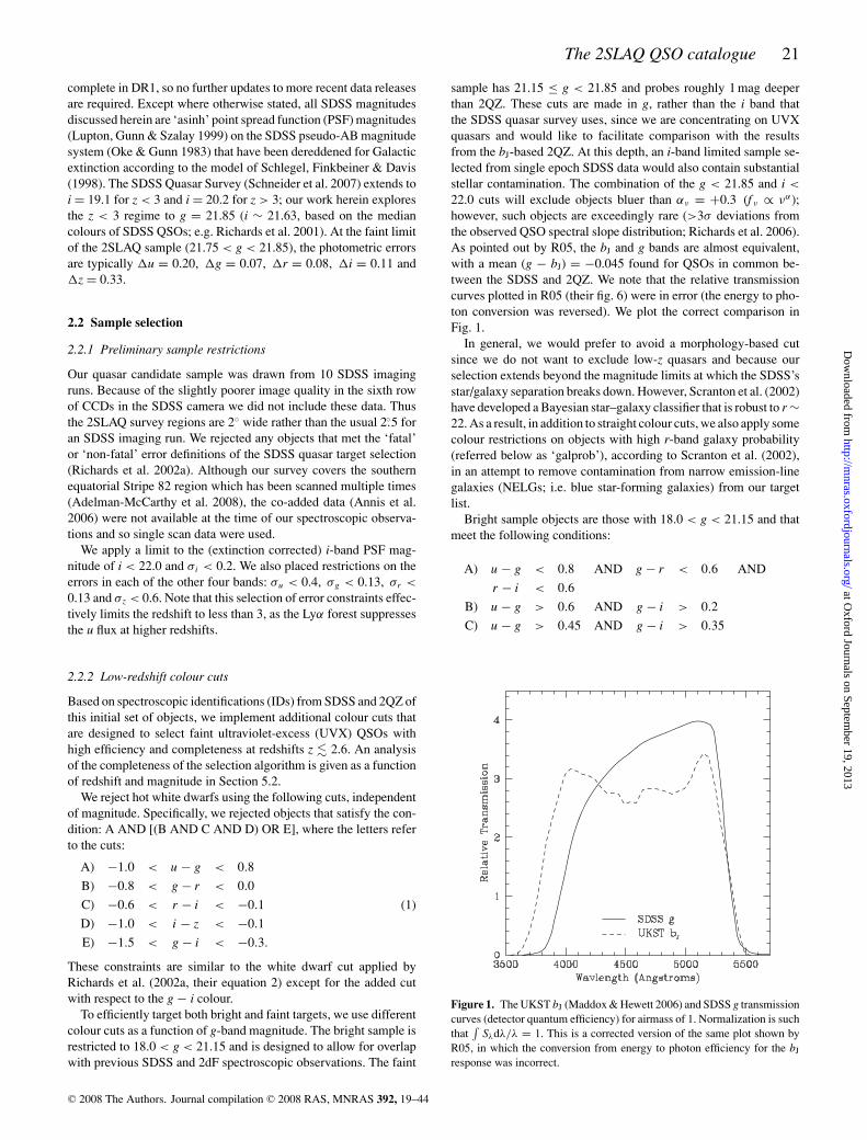
22.0 cuts will exclude objects bluer than αν = +0.3 (f ν ∝ να);however, such objects are exceedingly rare (>3σ deviations fromthe observed QSO spectral slope distribution; Richards et al. 2006).As pointed out by R05, the bJ and g bands are almost equivalent,with a mean (g − bJ) = −0.045 found for QSOs in common be-tween the SDSS and 2QZ. We note that the relative transmissioncurves plotted in R05 (their fig. 6) were in error (the energy to pho-ton conversion was reversed). We plot the correct comparison inFig. 1.
In general, we would prefer to avoid a morphology-based cutsince we do not want to exclude low-z quasars and because ourselection extends beyond the magnitude limits at which the SDSS’sstar/galaxy separation breaks down. However, Scranton et al. (2002)have developed a Bayesian star–galaxy classifier that is robust to r ∼22. As a result, in addition to straight colour cuts, we also apply somecolour restrictions on objects with high r-band galaxy probability(referred below as ‘galprob’), according to Scranton et al. (2002),in an attempt to remove contamination from narrow emission-linegalaxies (NELGs; i.e. blue star-forming galaxies) from our targetlist.
Bright sample objects are those with 18.0 < g < 21.15 and thatmeet the following conditions:
A) u − g < 0.8 AND g − r < 0.6 AND
r − i < 0.6
B) u − g > 0.6 AND g − i > 0.2
C) u − g > 0.45 AND g − i > 0.35
Figure 1. The UKST bJ (Maddox & Hewett 2006) and SDSS g transmissioncurves (detector quantum efficiency) for airmass of 1. Normalization is suchthat
∫Sλdλ/λ = 1. This is a corrected version of the same plot shown by
R05, in which the conversion from energy to photon efficiency for the bJ
response was incorrect.
C© 2008 The Authors. Journal compilation C© 2008 RAS, MNRAS 392, 19–44
at Oxford Journals on Septem
ber 19, 2013http://m
nras.oxfordjournals.org/D
ownloaded from
22 S. M. Croom et al.
D) galprob > 0.99 AND u − g > 0.2 AND
g − r > 0.25 AND r − i < 0.3
E) galprob > 0.99 AND u − g > 0.45
(2)
in the combination A AND (NOT B) AND (NOT C) AND (NOTD) AND (NOT E), where cut A selects UVX objects, cuts B andC eliminate faint F stars whose metallicity and errors push themblueward into the quasar regime and cuts D and E remove NELGsthat appear extended in the r band. Among the bright sample objects,those with g > 20.5 were given priority in terms of fibre assignment(see Section 3.2).
Faint sample objects are those with 21.15 ≤ g < 21.85 and thatmeet the following conditions:
A) u − g < 0.8 AND g − r < 0.5 AND
r − i < 0.6
B) u − g > 0.5 AND g − i > 0.15
C) u − g > 0.4 AND g − i > 0.3
D) u − g > 0.2 AND g − i > 0.45
E) galprob > 0.99 AND g − r > 0.3
(3)
in the combination A AND (NOT B) AND (NOT C) AND (NOTD) AND (NOT E), where cut A selects UVX objects, cuts B, C andD eliminate faint F stars whose metallicity and errors push themblueward into the quasar regime and cut E removes NELGs. Thesefaint cuts are more restrictive than the bright cuts to avoid significantcontamination from main-sequence stars that will enter the sampleas a result of larger errors at fainter magnitudes. The low-redshiftcolour cuts (u − g and g − i) are shown in Fig. 12 (see also fig. 1of R05).
2.2.3 High-redshift colour cuts
In addition to the main low-redshift (z � 2.6) sample describedabove, we also target a sample of higher redshift QSO candidates,analogous to the high-redshift sample selected in the main SDSSQSO survey which selected QSOs up to z � 5.4 at i < 20.2 (Richardset al. 2002a). The 2SLAQ high-redshift sample was limited toi < 21.0 and an additional constraint that σz < 0.4 was appliedto the z-band photometry. We then selected candidates in three red-shift intervals. QSO candidates at redshift �3.0–3.5 satisfied thefollowing cuts
σr < 0.13 AND
u > 20.6 AND
u − g > 1.5 AND
g − r < 1.2 AND
r − i < 0.3 AND
i − z > −1.0 AND
g − r < 0.44(u − g) − 0.76.
(4)
For the redshift range �3.5–4.5, this selection becomes
A) σr < 0.2
B) u − g > 1.5 OR u > 20.6
C) g − r > 0.7
D) g − r > 2.8 OR r − i < 0.44(g − r)
− 0.558
E) i − z < 0.25 AND i − z > −1.0,
(5)
in the combination A AND B AND C AND D AND E. For theredshifts above �4.5, we use
u > 21.5 AND
g > 21.0 AND
r − i > 0.6 AND
i − z > −1.0 AND
i − z < 0.52 (r − i) − 0.762.
(6)
These samples have a high degree of contamination from the stellarlocus due to photometric errors. These candidates were thereforetargeted at a lower priority than the main low-redshift sample, andwe do not present a detailed analysis of completeness for the high-redshift sample.
2.3 Survey area
The survey was targeted along the two equatorial regions fromthe SDSS imaging data. In the North Galactic Cap, we selectedfive disjoint regions along δ � 0◦ which contain the best qualityimaging data. These are denoted as regions a, b, c, d and e, aslisted in Table 1. In the South Galactic Cap, we targeted a singlecontiguous region, denoted as ‘s’. The 10 SDSS imaging runs usedare listed in Table 2, along with the 2SLAQ regions to which theycontribute. The 2SLAQ area completely overlaps with the brighterSDSS QSO survey (e.g. Schneider et al. 2007). There is partialoverlap with the 2QZ (C04) in the North Galactic Cap, with the2QZ covering the RA range 148◦ < αJ2000 < 223◦.
Table 1. Coordinates of the 2SLAQ survey regions.
2SLAQ RA (J2000) Dec. (J2000)region Min Max Min Max
a 123.0 144.0 −1.259 0.840b 150.0 168.0 −1.259 0.840c 185.0 193.0 −1.259 0.840d 197.0 214.0 −1.259 0.840e 218.0 230.0 −1.259 0.840s 309.0 59.70 −1.259 0.840
Table 2. SDSS imaging runs used for 2SLAQ targetselection. We list the run number, modified Julian date(MJD) of observation and the 2SLAQ regions thateach run contributes to. Note that runs can contributeto more than one 2SLAQ region.
SDSS run MJD 2SLAQ regions
752 51258 c, d, e756 51259 a, b, c, d, e1239 51607 a2141 51962 b2583 52172 s2659 52197 s2662 52197 s2738 52234 s3325 52522 s3388 52558 s
C© 2008 The Authors. Journal compilation C© 2008 RAS, MNRAS 392, 19–44
at Oxford Journals on Septem
ber 19, 2013http://m
nras.oxfordjournals.org/D
ownloaded from
The 2SLAQ QSO catalogue 23
3 SPECTRO SCOPIC OBSERVATIONS
3.1 Instrumental setup
Spectroscopic observations of the input catalogue were made withthe 2dF instrument at the AAT (Lewis et al. 2002). The 2dF instru-ment is a multifibre spectrograph which can obtain simultaneousspectra of up to 400 objects over a 2◦ diameter field of view, andis located at the prime focus of the telescope. Fibres are roboti-cally positioned within the field of view and fed to two identicalspectrographs (200 fibres each). Two field plates and a tumblingsystem allow one field to be observed while a second is beingconfigured, reducing downtime between fields to a minimum. Thespectrographs each contain a Tektronix 1024 × 1024 CCD with24 μm pixel.
Observations of QSOs and LRGs were combined by using 200fibres for each sample and sending these to separate spectrographs.QSO targets were sent to spectrograph 1 which contained a low-resolution 300B grating with a central wavelength of 5800 Å. LRGtargets were directed to spectrograph 2 with a higher resolution600V grating centred at 6150 Å (see Cannon et al. 2006 for furtherdetails of the LRG sample). The 300B grating produces a disper-sion of 4.3 Å pixel−1, giving an instrumental resolution of 9 Å. Thespectra covered the wavelength range 3700–7900 Å.
3.2 Target configuration and priority
The 2dF CONFIGURE program (Shortridge & Ramage 2003) was usedto allocate specific fibres to objects. This software takes an input listof prioritized positions (including guide fibres and target positions)and through an iterative scheme allocates fibres, producing a sec-ond file which is passed to the control software for the 2dF roboticpositioner. For the 2SLAQ observing programme, minor modifica-tions to the CONFIGURE software were made to allow (i) fibres fromdifferent spectrographs to be allocated to different samples and (ii)different central wavelengths for each spectrograph. We also car-ried out a detailed analysis of the spatial variation of configuredtarget density across the 2dF field. This showed that the algorithmcould, in certain circumstances, impart considerable structure onthe distribution of targets. The main effects seen were a deficit ofobjects near the centre of the field (<0.25◦ radius) in high-densityfields (where the number of targets is greater than the number offibres) and systematics related to the ordering of targets. To addressthese issues, the targets were randomized and randomly resampledso that the highest priority targets had a surface density of 70 deg−2.We note that these issues have since been fully addressed byMiszalski et al. (2006) using a simulated annealing algorithm; how-ever, 2SLAQ observations were carried out prior to this work.
Our most important targets were given higher priority in the fibreconfiguration process. These priorities are summarized in Table 3.LRGs were given highest priority because they have a lower surfacedensity than the QSO candidates. Our highest priority QSO targetshad g > 20.5 and were given a priority of 6. The surface densityof these targets was significantly higher than the ∼70 deg−2 thatcan be configured with the available fibres and so were randomlyresampled. The remaining g > 20.5 QSOs (not selected in therandom sampling) had their priority set to 5. The high-redshiftQSO candidates had their priorities set to 4 and the bright QSOcandidates (g < 20.5) had priority of 3. If a 2SLAQ-selected sourcealready had a high-quality spectroscopic observation from either2QZ or SDSS, its priority was set to 1 (lowest on a scale of 1–9)
Table 3. Configuration priorities for 2SLAQ targets.9 is the highest priority, while 1 is the lowest.
Sample Priority
Guide stars 9LRG (main) random 8LRG (main) remainder 7QSOs (g > 20.5) random 6QSOs (g > 20.5) remainder 5LRG(extras)+high-z QSOs 4QSOs (g < 20.5) 3Previously observed 1
in the 2dF configuration (i.e. it was observed only if no other targetwas available).
3.3 Tiling of 2dF fields
Given the geometry of the imaging area (strips between 10◦ and110◦ long, which are all 2◦ wide), it was sensible to employ asimple tiling pattern to cover the 2SLAQ regions. Each circular2dF field was spaced along the strip at intervals of 1.2◦ in RA.In some cases, field centres were shifted slightly to optimize theirpositions (e.g. at the end of survey regions). Some of the first fieldsobserved (2003 February–April) had a smaller spacing of 1◦. The1.2◦ spacing produced a near optimal balance between coverageand completeness for both the QSOs and LRGs. This approachalso provides some overlap between adjacent fields. The 2dF fieldof view has a radius of 1.05◦. For most observations, configuredobjects were constrained to lie within a circle of exactly 1.05◦ radius;however, early observations did not apply this constraint (2003February–September). As a result, 19 2SLAQ objects (including 10good quality QSOs) were observed marginally outside the nominalsurvey region bounded by the intersection of all the observed fieldseach with radius 1.05◦. This can be caused by the effects suchas atmospheric refraction which distorts the field of view at high
Table 4. 2SLAQ observed objects which are outside of the nominal surveylimits bounded by the intersection of 1.05◦ radius 2dF fields of view.
Name RA (J2000) Dec. (J2000)(◦) (◦)
J005128.22+004447.8 12.867619 0.746637J010159.56+004820.2 15.498189 0.805634J010423.79+004029.8 16.099131 0.674965J022526.32−011434.3 36.359680 −1.242874J081233.10+004643.0 123.137909 0.778604J081238.23+004713.2 123.159286 0.786992J081938.22−011052.6 124.909256 −1.181273J100705.00−010904.9 151.770844 −1.151354J123158.37+004635.6 187.993195 0.776566J123448.89+004752.3 188.703705 0.797856J134054.18+004911.9 205.225769 0.819972J143313.87−011501.2 218.307800 −1.250338J143620.20+004529.6 219.084152 0.758220J143922.06−011215.0 219.841934 −1.204170J144007.84+004156.2 220.032654 0.698939J211844.76+003134.4 319.686523 0.526249J211955.31+004301.6 319.980469 0.717123J212129.68+004827.1 320.373688 0.807553J214859.57+004439.5 327.248230 0.744307
C© 2008 The Authors. Journal compilation C© 2008 RAS, MNRAS 392, 19–44
at Oxford Journals on Septem
ber 19, 2013http://m
nras.oxfordjournals.org/D
ownloaded from
24 S. M. Croom et al.
airmass. These are included in the catalogue, but excluded in severalof the analyses below; the names of these sources are given inTable 4.
In order to maximize the yield from overlapping fields, se-quences of alternating fields were generally observed first, with theinterleaved overlapping fields observed in a second pass. On thissecond pass, all targets which obtained high-quality IDs (quality 1;see Section 3.6) from previous observations were given the lowestpriority (priority 1), so that a minimal number of objects with ac-ceptable spectroscopic data were repeated. Even allowing for this,3317 objects have repeated observations. Approximately half ofthese were because the original spectrum was of low quality. Theother half were repeated because there was no higher priority tar-get accessible. These repeated spectra are useful in making internalchecks of completeness and consistency.
There are also a number of physical constraints on the config-uration of 2dF fields. In the 2SLAQ survey, the most apparent ofthese is that fibres are arranged around the edge of the field platesin blocks of 10. These blocks of 10 fibres go to alternating spec-trographs, such that there is a triangular region directly in front ofeach fibre block going to spectrograph 2 that fibres from spectro-graph 1 cannot access. This is because 2dF fibres are limited to amaximum off-radial angle of 14◦. The 20 small inaccessible trian-gles amount to a total area of 0.43 deg2. As a number of differentsamples are configured together in each field, the distribution ofother targets also influences the angular selection function within
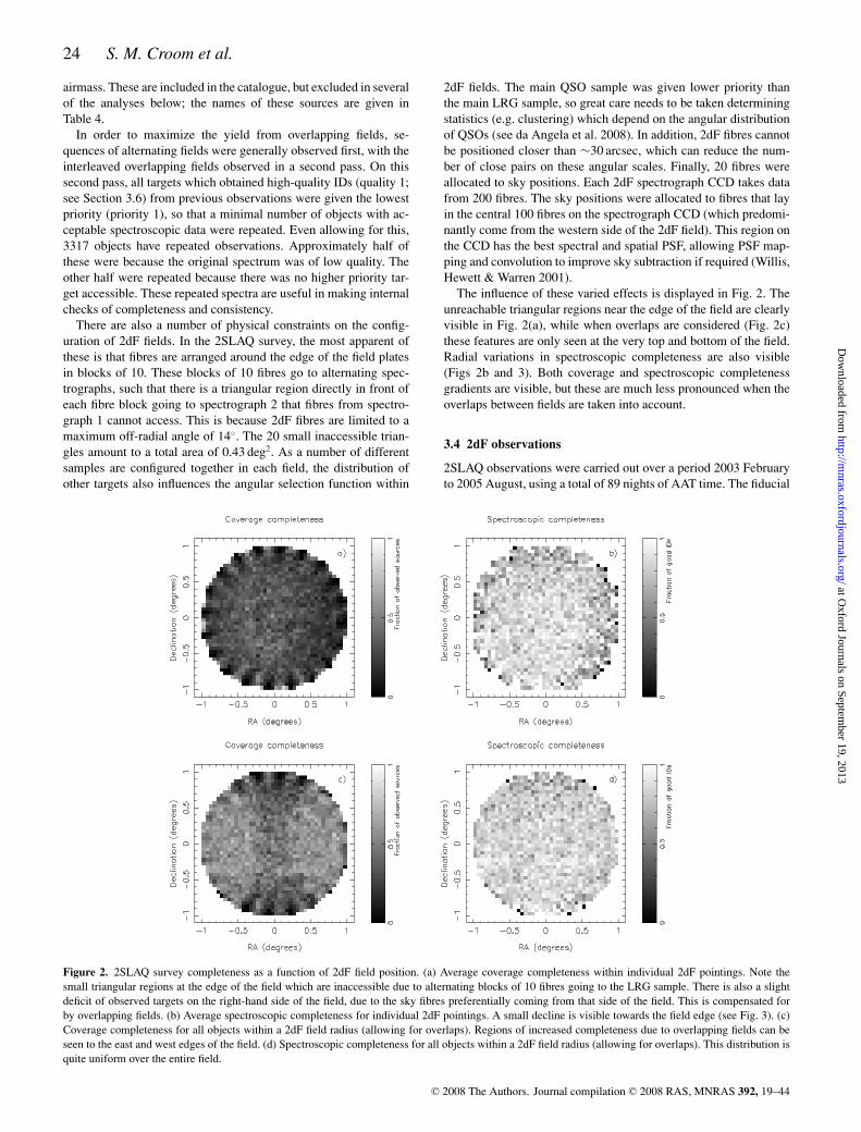
Figure 2. 2SLAQ survey completeness as a function of 2dF field position. (a) Average coverage completeness within individual 2dF pointings. Note thesmall triangular regions at the edge of the field which are inaccessible due to alternating blocks of 10 fibres going to the LRG sample. There is also a slightdeficit of observed targets on the right-hand side of the field, due to the sky fibres preferentially coming from that side of the field. This is compensated forby overlapping fields. (b) Average spectroscopic completeness for individual 2dF pointings. A small decline is visible towards the field edge (see Fig. 3). (c)Coverage completeness for all objects within a 2dF field radius (allowing for overlaps). Regions of increased completeness due to overlapping fields can beseen to the east and west edges of the field. (d) Spectroscopic completeness for all objects within a 2dF field radius (allowing for overlaps). This distribution isquite uniform over the entire field.
2dF fields. The main QSO sample was given lower priority thanthe main LRG sample, so great care needs to be taken determiningstatistics (e.g. clustering) which depend on the angular distributionof QSOs (see da Angela et al. 2008). In addition, 2dF fibres cannotbe positioned closer than ∼30 arcsec, which can reduce the num-ber of close pairs on these angular scales. Finally, 20 fibres wereallocated to sky positions. Each 2dF spectrograph CCD takes datafrom 200 fibres. The sky positions were allocated to fibres that layin the central 100 fibres on the spectrograph CCD (which predomi-nantly come from the western side of the 2dF field). This region onthe CCD has the best spectral and spatial PSF, allowing PSF map-ping and convolution to improve sky subtraction if required (Willis,Hewett & Warren 2001).
The influence of these varied effects is displayed in Fig. 2. Theunreachable triangular regions near the edge of the field are clearlyvisible in Fig. 2(a), while when overlaps are considered (Fig. 2c)these features are only seen at the very top and bottom of the field.Radial variations in spectroscopic completeness are also visible(Figs 2b and 3). Both coverage and spectroscopic completenessgradients are visible, but these are much less pronounced when theoverlaps between fields are taken into account.
3.4 2dF observations
2SLAQ observations were carried out over a period 2003 Februaryto 2005 August, using a total of 89 nights of AAT time. The fiducial
C© 2008 The Authors. Journal compilation C© 2008 RAS, MNRAS 392, 19–44
at Oxford Journals on Septem
ber 19, 2013http://m
nras.oxfordjournals.org/D
ownloaded from
The 2SLAQ QSO catalogue 25
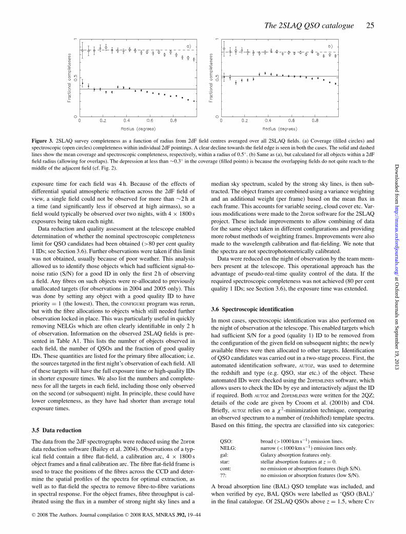
Figure 3. 2SLAQ survey completeness as a function of radius from 2dF field centres averaged over all 2SLAQ fields. (a) Coverage (filled circles) andspectroscopic (open circles) completeness within individual 2dF pointings. A clear decline towards the field edge is seen in both the cases. The solid and dashedlines show the mean coverage and spectroscopic completeness, respectively, within a radius of 0.5◦. (b) Same as (a), but calculated for all objects within a 2dFfield radius (allowing for overlaps). The depression at less than ∼0.3◦ in the coverage (filled points) is because the overlapping fields do not quite reach to themiddle of the adjacent field (cf. Fig. 2).
exposure time for each field was 4 h. Because of the effects ofdifferential spatial atmospheric refraction across the 2dF field ofview, a single field could not be observed for more than ∼2 h ata time (and significantly less if observed at high airmass), so afield would typically be observed over two nights, with 4 × 1800 sexposures being taken each night.
Data reduction and quality assessment at the telescope enableddetermination of whether the nominal spectroscopic completenesslimit for QSO candidates had been obtained (>80 per cent quality1 IDs; see Section 3.6). Further observations were taken if this limitwas not obtained, usually because of poor weather. This analysisallowed us to identify those objects which had sufficient signal-to-noise ratio (S/N) for a good ID in only the first 2 h of observinga field. Any fibres on such objects were re-allocated to previouslyunallocated targets (for observations in 2004 and 2005 only). Thiswas done by setting any object with a good quality ID to havepriority = 1 (the lowest). Then, the CONFIGURE program was rerun,but with the fibre allocations to objects which still needed furtherobservation locked in place. This was particularly useful in quicklyremoving NELGs which are often clearly identifiable in only 2 hof observation. Information on the observed 2SLAQ fields is pre-sented in Table A1. This lists the number of objects observed ineach field, the number of QSOs and the fraction of good qualityIDs. These quantities are listed for the primary fibre allocation; i.e.the sources targeted in the first night’s observation of each field. Allof these targets will have the full exposure time or high-quality IDsin shorter exposure times. We also list the numbers and complete-ness for all the targets in each field, including those only observedon the second (or subsequent) night. In principle, these could havelower completeness, as they have had shorter than average totalexposure times.
3.5 Data reduction
The data from the 2dF spectrographs were reduced using the 2DFDR
data reduction software (Bailey et al. 2004). Observations of a typ-ical field contain a fibre flat-field, a calibration arc, 4 × 1800 sobject frames and a final calibration arc. The fibre flat-field frame isused to trace the positions of the fibres across the CCD and deter-mine the spatial profiles of the spectra for optimal extraction, aswell as to flat-field the spectra to remove fibre-to-fibre variationsin spectral response. For the object frames, fibre throughput is cal-ibrated using the flux in a number of strong night sky lines and a
median sky spectrum, scaled by the strong sky lines, is then sub-tracted. The object frames are combined using a variance weightingand an additional weight (per frame) based on the mean flux ineach frame. This accounts for variable seeing, cloud cover etc. Var-ious modifications were made to the 2DFDR software for the 2SLAQproject. These include improvements to allow combining of datafor the same object taken in different configurations and providingmore robust methods of weighting frames. Improvements were alsomade to the wavelength calibration and flat-fielding. We note thatthe spectra are not spectrophotometrically calibrated.
Data were reduced on the night of observation by the team mem-bers present at the telescope. This operational approach has theadvantage of pseudo-real-time quality control of the data. If therequired spectroscopic completeness was not achieved (80 per centquality 1 IDs; see Section 3.6), the exposure time was extended.
3.6 Spectroscopic identification
In most cases, spectroscopic identification was also performed onthe night of observation at the telescope. This enabled targets whichhad sufficient S/N for a good (quality 1) ID to be removed fromthe configuration of the given field on subsequent nights; the newlyavailable fibres were then allocated to other targets. Identificationof QSO candidates was carried out in a two-stage process. First, theautomated identification software, AUTOZ, was used to determinethe redshift and type (e.g. QSO, star etc.) of the object. Theseautomated IDs were checked using the 2DFEMLINES software, whichallows users to check the IDs by eye and interactively adjust the IDif required. Both AUTOZ and 2DFEMLINES were written for the 2QZ;details of the code are given by Croom et al. (2001b) and C04.Briefly, AUTOZ relies on a χ 2-minimization technique, comparingan observed spectrum to a number of (redshifted) template spectra.Based on this fitting, the spectra are classified into six categories:
QSO: broad (>1000 km s−1) emission lines.NELG: narrow (<1000 km s−1) emission lines only.gal: Galaxy absorption features only.star: stellar absorption features at z = 0.cont: no emission or absorption features (high S/N).??: no emission or absorption features (low S/N).
A broad absorption line (BAL) QSO template was included, andwhen verified by eye, BAL QSOs were labelled as ‘QSO (BAL)’in the final catalogue. Of 2SLAQ QSOs above z = 1.5, where C IV
C© 2008 The Authors. Journal compilation C© 2008 RAS, MNRAS 392, 19–44
at Oxford Journals on Septem
ber 19, 2013http://m
nras.oxfordjournals.org/D
ownloaded from
26 S. M. Croom et al.
is visible in the observed spectrum, 171/4591 (3.7 per cent) areclassified as BALs. This is a lower limit to the total BAL fractionas we have not performed a consistent and quantitative analysis forBALs [e.g. using the BALnicity index of Weymann et al. (1991)].As a part of the ID process, each spectrum is assigned a quality forthe ID and redshift as follows:
Quality 1: high-quality ID or redshift.Quality 2: poor-quality ID or redshift.Quality 3: no ID or redshift assignment.
The quality flag was determined independently for the ID and red-shift of an object. For example, a quality 1 QSO ID could havea quality 1 or 2 redshift. A quality 1 ID is assigned if multiplespectral features are seen. QSOs with only a strong broad Mg II
emission line are also given a quality 1 ID. A quality 2 ID is givenif there is only a single spectral feature, or features of only marginalsignificance. The reliability of the different qualities is assessedbelow.
4 TH E 2 S L AQ Q S O C ATA L O G U E
In this section, we discuss the 2SLAQ QSO catalogue. The formatof the catalogue is given in Table 5. It is available in electronic formfrom http://www.2slaq.info/. A second table which contains detailsof multiply observed sources is also available. The format for thislist is given by Table 6. The catalogue includes SDSS photometry(PSF magnitudes) and star–galaxy classification. Note that some ofthe SDSS values, such as SDSSid number, are specific to DR1, andcan change in subsequent data releases. Where available, we alsoinclude SDSS and 2QZ spectroscopic IDs for 2SLAQ sources. Forthe 2SLAQ spectroscopy, we list the best measured redshift, theobject ID (e.g. QSO, NELG etc.) and the redshift/ID quality. Forobjects with repeated observations, the catalogue lists the parame-ters for the best spectrum, which is selected based on redshift/IDquality and S/N. As part of the data release, we also provide theparameters for all other repeated observations. We include a numberof observational details such as date, field, fibre number and S/N(averaged in the 4000 to 5000 Å band). Objects which were onlyconfigured in a field on the second or subsequent nights have beengiven fibre numbers greater than 200. The dmag entry is the dif-ference between the observed fibre magnitude (at 4000 to 5000 Å)and the SDSS PSF magnitude in the g band. This is zero pointed tothe mean difference in each field, and so gives an estimate of whichobjects were brighter or fainter than their SDSS photometry wouldpredict. We matched to the ROSAT All Sky Survey (RASS; Vogeset al. 1999, 2000) with a maximum matching radius of 30 arcsec.Non-matches are indicated by zero flux in the RASS column. Wealso searched for matches to the Faint Images of the Radio Sky atTwenty-cm (FIRST) radio survey (Becker, White & Helfand 1995).Given that the radio morphologies can often be complex and ex-tended, we first made a list of all 2SLAQ sources which had a radiomatch within 1 arcmin. Each of these matches was then examinedby eye to determine whether it was a true match. If multiple compo-nents were present, the flux from these was summed. The FIRSTextflag is then set based on the morphology, either unresolved (1), sin-gle extended source (2) or multiple source (3). The flag is set to zerofor a non-detection. The final entry in the catalogue is reserved forany comments that are made on the 2SLAQ spectrum in the processof manual checking of the data.
As well as the catalogue, we also make public all the spectra ofobjects targeted as part of 2SLAQ observations. These are availableas individual FITS format spectra and include repeated observations.
A small fraction of spectra have bad ‘fringing’ caused by a damagedfibre, showing up as a strong oscillation as a function of wavelength.These are noted as such in the comments field of the catalogue.Access to the spectra is via the web site http://www.2slaq.info/.
We now discuss the catalogue composition and the robustness ofthe IDs and redshifts.
4.1 Catalogue composition
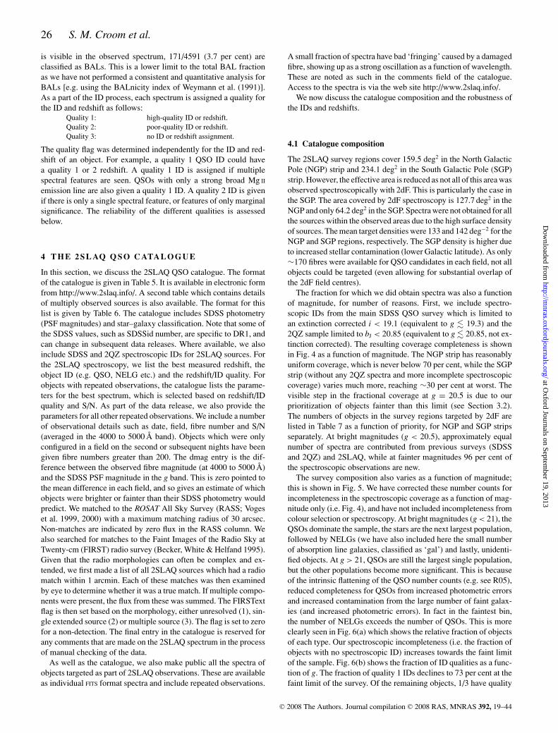
The 2SLAQ survey regions cover 159.5 deg2 in the North GalacticPole (NGP) strip and 234.1 deg2 in the South Galactic Pole (SGP)strip. However, the effective area is reduced as not all of this area wasobserved spectroscopically with 2dF. This is particularly the case inthe SGP. The area covered by 2dF spectroscopy is 127.7 deg2 in theNGP and only 64.2 deg2 in the SGP. Spectra were not obtained for allthe sources within the observed areas due to the high surface densityof sources. The mean target densities were 133 and 142 deg−2 for theNGP and SGP regions, respectively. The SGP density is higher dueto increased stellar contamination (lower Galactic latitude). As only∼170 fibres were available for QSO candidates in each field, not allobjects could be targeted (even allowing for substantial overlap ofthe 2dF field centres).
The fraction for which we did obtain spectra was also a functionof magnitude, for number of reasons. First, we include spectro-scopic IDs from the main SDSS QSO survey which is limited toan extinction corrected i < 19.1 (equivalent to g � 19.3) and the2QZ sample limited to bJ < 20.85 (equivalent to g � 20.85, not ex-tinction corrected). The resulting coverage completeness is shownin Fig. 4 as a function of magnitude. The NGP strip has reasonablyuniform coverage, which is never below 70 per cent, while the SGPstrip (without any 2QZ spectra and more incomplete spectroscopiccoverage) varies much more, reaching ∼30 per cent at worst. Thevisible step in the fractional coverage at g = 20.5 is due to ourprioritization of objects fainter than this limit (see Section 3.2).The numbers of objects in the survey regions targeted by 2dF arelisted in Table 7 as a function of priority, for NGP and SGP stripsseparately. At bright magnitudes (g < 20.5), approximately equalnumber of spectra are contributed from previous surveys (SDSSand 2QZ) and 2SLAQ, while at fainter magnitudes 96 per cent ofthe spectroscopic observations are new.
The survey composition also varies as a function of magnitude;this is shown in Fig. 5. We have corrected these number counts forincompleteness in the spectroscopic coverage as a function of mag-nitude only (i.e. Fig. 4), and have not included incompleteness fromcolour selection or spectroscopy. At bright magnitudes (g < 21), theQSOs dominate the sample, the stars are the next largest population,followed by NELGs (we have also included here the small numberof absorption line galaxies, classified as ‘gal’) and lastly, unidenti-fied objects. At g > 21, QSOs are still the largest single population,but the other populations become more significant. This is becauseof the intrinsic flattening of the QSO number counts (e.g. see R05),reduced completeness for QSOs from increased photometric errorsand increased contamination from the large number of faint galax-ies (and increased photometric errors). In fact in the faintest bin,the number of NELGs exceeds the number of QSOs. This is moreclearly seen in Fig. 6(a) which shows the relative fraction of objectsof each type. Our spectroscopic incompleteness (i.e. the fraction ofobjects with no spectroscopic ID) increases towards the faint limitof the sample. Fig. 6(b) shows the fraction of ID qualities as a func-tion of g. The fraction of quality 1 IDs declines to 73 per cent at thefaint limit of the survey. Of the remaining objects, 1/3 have quality
C© 2008 The Authors. Journal compilation C© 2008 RAS, MNRAS 392, 19–44
at Oxford Journals on Septem
ber 19, 2013http://m
nras.oxfordjournals.org/D
ownloaded from
The 2SLAQ QSO catalogue 27
Table 5. Format for the 2SLAQ QSO catalogue. The format entries are based on the standard FORTRAN format descriptors. The full tableis available in the electronic version of the journal.
Field Format Description
Name a19 IAU format object namePriority i1 Configuration priority for 2dFRA f10.6 RA J2000 in decimal degreesDec. f10.6 Dec J2000 in decimal degreesSDSSrun i4 SDSS run numberSDSSrerun i2 SDSS rerun numberSDSScamcol i1 SDSS camera columnSDSSfield i3 SDSS fieldSDSSid i4 SDSS object id within a fieldSDSSrow f8.3 SDSS CCD Y position (pixel)SDSScol f8.3 SDSS CCD X position (pixel)um f6.3 SDSS PSF magnitude in u band (no extinction correction)gm f6.3 SDSS PSF magnitude in g band (no extinction correction)rm f6.3 SDSS PSF magnitude in r band (no extinction correction)im f6.3 SDSS PSF magnitude in i band (no extinction correction)zm f6.3 SDSS PSF magnitude in z band (no extinction correction)umerr f5.3 SDSS PSF magnitude error in u bandgmerr f5.3 SDSS PSF magnitude error in g bandrmerr f5.3 SDSS PSF magnitude error in r bandimerr f5.3 SDSS PSF magnitude error in i bandzmerr f5.3 SDSS PSF magnitude error in z bandumred f5.3 Extinction in u band (mag)gmred f5.3 Extinction in g band (mag)rmred f5.3 Extinction in r band (mag)imred f5.3 Extinction in i band (mag)zmred f5.3 Extinction in z band (mag)sg f8.5 SDSS Bayesian star–galaxy classification probabilitymorph i1 SDSS Object image morphology classification 3 = galaxy, 6 = starzemsdss f7.4 SDSS spectroscopic redshifttypesdss a7 SDSS spectroscopic ID typequalsdss f6.4 SDSS spectroscopic qualitybj f5.2 2QZ bJ magnitude (Smith et al. 2005)zem2df f7.4 2QZ spectroscopic redshift (C04)type2df a8 2QZ spectroscopic ID type (C04)qual2df i2 2QZ spectroscopic ID/redshift quality (C04)name2df a19 2QZ IAU format namez f7.4 2SLAQ spectroscopic redshiftqual i2 2SLAQ spectroscopic quality (ID quality × 10 + redshift quality)ID a10 2SLAQ spectroscopic ID (i.e. QSO, NELG, star etc.)date i6 2SLAQ spectroscopic observation date (YYMMDD)fld a3 2SLAQ spectroscopic fieldfib i3 2SLAQ spectroscopic fibre numberS/N f7.2 2SLAQ spectroscopic S/N in a 4000–5000 Å banddmag f6.2 2SLAQ (gm mag) - (fibre mag) relative to mean z.p. in fieldRASS f7.4 RASS X-ray flux, (×10−13 erg s −1 cm−2)FIRST f6.1 FIRST 1.4 GHz Radio flux (mJy)FIRSText i1 FIRST morphology; 0 = no detection, 1 = unresolved, 2 = extended, 3 = multiplecomment a20 2SLAQ comment on spectrum
2 IDs and 2/3 have quality 3 IDs (the poorest). For most analysesin this paper, only quality 1 IDs are used.
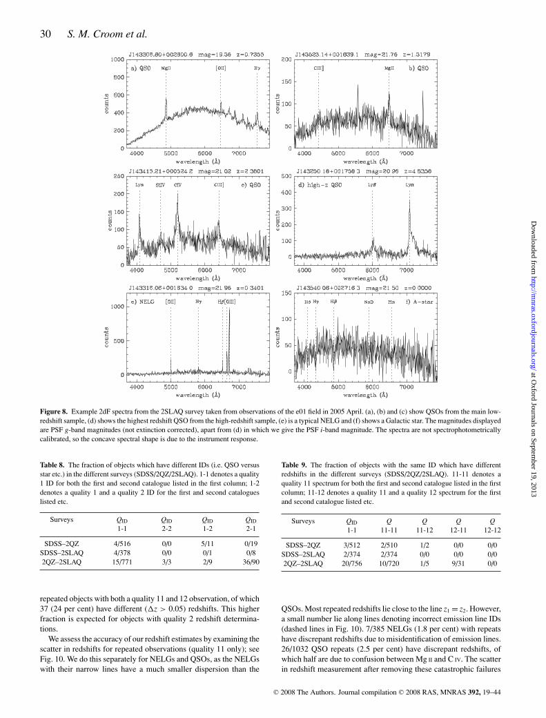
The redshift distribution of the main low-redshift QSO sampleis shown in Fig. 7 as the solid line. The number of QSOs is rela-tively constant between z � 0.8 and 2.2, declining towards lowerand higher redshift. The high-redshift sample (Section 2.2.3) pri-marily samples the redshift range between z � 2.8 and 4.0, with thehighest redshift QSO being J143250.16+001756.3 at z = 4.8356.The NELGs (including some absorption line galaxies) are peakedat low redshift, with a tail of objects to z � 1. Example 2SLAQ
spectra, including a range of QSO redshifts and magnitudes as wellas a NELG and a Galactic star, are shown in Fig. 8.
4.2 Repeatability of identifications and redshifts
A critical test of the quality of the catalogue is to assess the reli-ability and repeatability of our IDs and redshifts. We can do thisboth internally, using repeated observations, and externally usingcomparisons to other catalogues. In particular, we have 2SLAQspectra for objects which also have SDSS and 2QZ spectra
C© 2008 The Authors. Journal compilation C© 2008 RAS, MNRAS 392, 19–44
at Oxford Journals on Septem
ber 19, 2013http://m
nras.oxfordjournals.org/D
ownloaded from
28 S. M. Croom et al.
Table 6. Format for the 2SLAQ QSO repeated objects catalogue. This lists the observational details and IDs for each object thatwas observed multiple times. One observation is given per line and they are given in order of the date of observation. The formatentries are based on the standard FORTRAN format descriptors. The full table is available in the electronic version of the journal.
Field Format Description
Name a19 IAU format object namez f7.4 2SLAQ spectroscopic redshiftqual i2 2SLAQ spectroscopic quality (ID quality × 10 + redshift quality)ID a10 2SLAQ spectroscopic ID (i.e. QSO, NELG, star etc.)date i6 2SLAQ spectroscopic observation date (YYMMDD)fld a3 2SLAQ spectroscopic fieldfib i3 2SLAQ spectroscopic fibre numberS/N f7.2 2SLAQ spectroscopic S/N in a 4000–5000 Å banddmag f6.2 2SLAQ (gm mag) - (fibre mag) relative to mean z.p. in fieldobs i1 Number of observation for this object.Comment a20 2SLAQ comment on spectrum
Figure 4. The fractional spectroscopic coverage as a function of g-bandmagnitude (extinction corrected) for the NGP (solid histogram) and SGP(dashed histogram) strips of the 2SLAQ QSO sample. Error bars are Poisso-nian. In this plot, we include objects which have previously been identifiedby the 2QZ and SDSS surveys. The lower coverage in the SGP strip isbecause a smaller fraction of overlapping fields were observed in this strip.Also this region does not include 2QZ objects. The increase towards brightmagnitudes is due to the inclusion of SDSS IDs and the step at g = 20.5 isdue to our prioritization of sources fainter than this limit.
available. In this external check, it is worth noting that the over-lap between SDSS/2QZ and 2SLAQ is only at the bright endof the sample, where IDs are inherently more reliable. Secondly,the 2QZ is only nominally an external check, as the data acqui-sition, reduction and analysis for 2QZ and 2SLAQ are almostidentical.
We start by assessing the relative reliability of the IDs betweensurveys. In Table 8, we list the number of objects with differentquality IDs in more than one sample, compared to the number forwhich that ID disagrees between samples. For good quality IDs(QID = 1) in two samples, we find that 4/516 objects disagree be-tween SDSS and 2QZ (0.8 ± 0.4 per cent), 4/378 between SDSSand 2SLAQ (1.1 ± 0.5 per cent) and 15/771 between 2QZ and2SLAQ (2.0 ± 0.5 per cent). By visually examining the spectra,we find that for all four SDSS-2QZ discrepancies the SDSS IDis correct. For the SDSS-2SLAQ comparison we find the SDSSID to be corrected in three cases and the 2SLAQ ID to be cor-rect in one case. All four objects have the same redshift in both
Table 7. The number of objects within 2SLAQ 2dF fields (Nobj) as a functionof priority. We shown this separately for the NGP and SGP strips. We alsolist the number of objects in the same regions with spectroscopy fromSDSS (DR4), 2QZ and 2SLAQ as well as the total number of objects withspectroscopic observations (Nobs). Because some objects were observed bymore than one of SDSS, 2QZ and 2SLAQ, Nobs is not equal to the sum of theother columns. Also, we do not include the 19 objects that are outside ourformal 2SLAQ limits (see Table 4). Fobs is the fraction of objects observed,i.e. Nobs/Nobj. Aobs is the effective area for each sample i.e. (surveyed area)×Fobs.
Pri. Nobj NSDSS N2QZ N2SLAQ Nobs Fobs Aobs
(deg2)
3-NGP 4795 1054 2351 2015 3893 0.812 102.604-NGP 795 18 1 459 474 0.576 75.345-NGP 4567 0 62 3321 3338 0.731 92.366-NGP 6908 6 501 5733 6042 0.875 110.53
3-SGP 2351 553 0 561 1051 0.447 28.384-SGP 23 5 0 7 12 0.522 33.125-SGP 2884 0 0 1584 1584 0.549 34.866-SGP 3413 17 0 2627 2642 0.774 49.13
samples, and the disagreement is due to classification as NELGor QSO. For the 2QZ-2SLAQ comparison, we found five casesin which the 2QZ ID was correct and 10 cases were the 2SLAQID was correct. Of these 10, eight were low S/N objects in 2QZwrongly classified as stars. If we compare lower quality IDs, we findthat, as expected, the repeatability is poorer (final three columns inTable 8).
Next, we check the external reliability of the redshift estimates.We search for objects identified in more than one sample that havethe same ID (with QID = 1) but a redshift difference of greater than�z = 0.05 (chosen to include only those objects with catastrophicfailures in redshift). This resulted in 3/512 for the SDSS-2QZ com-parison, 2/374 for the SDSS-2SLAQ comparison and 20/756 in the2QZ-2SLAQ comparison. However for a number of objects, the red-shift was flagged as uncertain (i.e. Qz = 2). If we limit ourselves toobjects with Q = 11 (i.e. QID = 1 and Qz = 1) then the fractions are2/510, 2/374 and 10/720, respectively (see Table 9). Visual assess-ment of the spectra for which there were discrepant redshifts showedthat the surveys scored 2-1 (SDSS-2QZ), 2-0 (SDSS-2SLAQ) and
C© 2008 The Authors. Journal compilation C© 2008 RAS, MNRAS 392, 19–44
at Oxford Journals on Septem
ber 19, 2013http://m
nras.oxfordjournals.org/D
ownloaded from
The 2SLAQ QSO catalogue 29
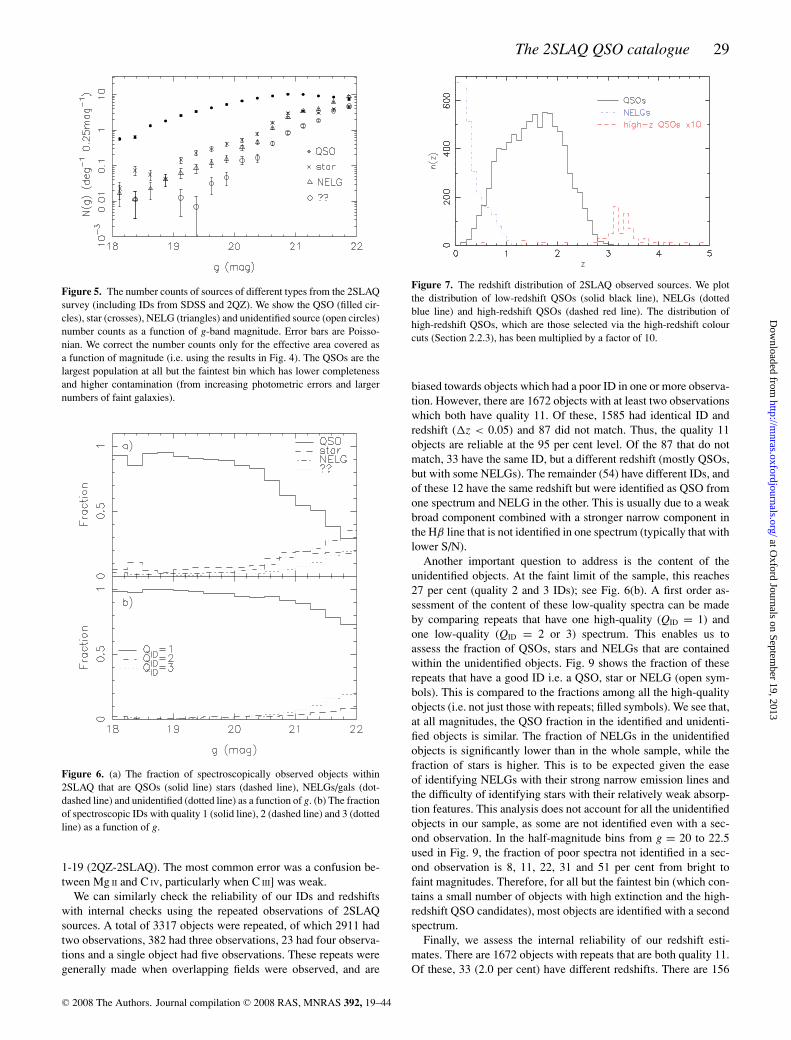
Figure 5. The number counts of sources of different types from the 2SLAQsurvey (including IDs from SDSS and 2QZ). We show the QSO (filled cir-cles), star (crosses), NELG (triangles) and unidentified source (open circles)number counts as a function of g-band magnitude. Error bars are Poisso-nian. We correct the number counts only for the effective area covered asa function of magnitude (i.e. using the results in Fig. 4). The QSOs are thelargest population at all but the faintest bin which has lower completenessand higher contamination (from increasing photometric errors and largernumbers of faint galaxies).
Figure 6. (a) The fraction of spectroscopically observed objects within2SLAQ that are QSOs (solid line) stars (dashed line), NELGs/gals (dot-dashed line) and unidentified (dotted line) as a function of g. (b) The fractionof spectroscopic IDs with quality 1 (solid line), 2 (dashed line) and 3 (dottedline) as a function of g.
1-19 (2QZ-2SLAQ). The most common error was a confusion be-tween Mg II and C IV, particularly when C III] was weak.
We can similarly check the reliability of our IDs and redshiftswith internal checks using the repeated observations of 2SLAQsources. A total of 3317 objects were repeated, of which 2911 hadtwo observations, 382 had three observations, 23 had four observa-tions and a single object had five observations. These repeats weregenerally made when overlapping fields were observed, and are
Figure 7. The redshift distribution of 2SLAQ observed sources. We plotthe distribution of low-redshift QSOs (solid black line), NELGs (dottedblue line) and high-redshift QSOs (dashed red line). The distribution ofhigh-redshift QSOs, which are those selected via the high-redshift colourcuts (Section 2.2.3), has been multiplied by a factor of 10.
biased towards objects which had a poor ID in one or more observa-tion. However, there are 1672 objects with at least two observationswhich both have quality 11. Of these, 1585 had identical ID andredshift (�z < 0.05) and 87 did not match. Thus, the quality 11objects are reliable at the 95 per cent level. Of the 87 that do notmatch, 33 have the same ID, but a different redshift (mostly QSOs,but with some NELGs). The remainder (54) have different IDs, andof these 12 have the same redshift but were identified as QSO fromone spectrum and NELG in the other. This is usually due to a weakbroad component combined with a stronger narrow component inthe Hβ line that is not identified in one spectrum (typically that withlower S/N).
Another important question to address is the content of theunidentified objects. At the faint limit of the sample, this reaches27 per cent (quality 2 and 3 IDs); see Fig. 6(b). A first order as-sessment of the content of these low-quality spectra can be madeby comparing repeats that have one high-quality (QID = 1) andone low-quality (QID = 2 or 3) spectrum. This enables us toassess the fraction of QSOs, stars and NELGs that are containedwithin the unidentified objects. Fig. 9 shows the fraction of theserepeats that have a good ID i.e. a QSO, star or NELG (open sym-bols). This is compared to the fractions among all the high-qualityobjects (i.e. not just those with repeats; filled symbols). We see that,at all magnitudes, the QSO fraction in the identified and unidenti-fied objects is similar. The fraction of NELGs in the unidentifiedobjects is significantly lower than in the whole sample, while thefraction of stars is higher. This is to be expected given the easeof identifying NELGs with their strong narrow emission lines andthe difficulty of identifying stars with their relatively weak absorp-tion features. This analysis does not account for all the unidentifiedobjects in our sample, as some are not identified even with a sec-ond observation. In the half-magnitude bins from g = 20 to 22.5used in Fig. 9, the fraction of poor spectra not identified in a sec-ond observation is 8, 11, 22, 31 and 51 per cent from bright tofaint magnitudes. Therefore, for all but the faintest bin (which con-tains a small number of objects with high extinction and the high-redshift QSO candidates), most objects are identified with a secondspectrum.
Finally, we assess the internal reliability of our redshift esti-mates. There are 1672 objects with repeats that are both quality 11.Of these, 33 (2.0 per cent) have different redshifts. There are 156
C© 2008 The Authors. Journal compilation C© 2008 RAS, MNRAS 392, 19–44
at Oxford Journals on Septem
ber 19, 2013http://m
nras.oxfordjournals.org/D
ownloaded from
30 S. M. Croom et al.
Figure 8. Example 2dF spectra from the 2SLAQ survey taken from observations of the e01 field in 2005 April. (a), (b) and (c) show QSOs from the main low-redshift sample, (d) shows the highest redshift QSO from the high-redshift sample, (e) is a typical NELG and (f) shows a Galactic star. The magnitudes displayedare PSF g-band magnitudes (not extinction corrected), apart from (d) in which we give the PSF i-band magnitude. The spectra are not spectrophotometricallycalibrated, so the concave spectral shape is due to the instrument response.
Table 8. The fraction of objects which have different IDs (i.e. QSO versusstar etc.) in the different surveys (SDSS/2QZ/2SLAQ). 1-1 denotes a quality1 ID for both the first and second catalogue listed in the first column; 1-2denotes a quality 1 and a quality 2 ID for the first and second catalogueslisted etc.
Surveys QID QID QID QID
1-1 2-2 1-2 2-1
SDSS–2QZ 4/516 0/0 5/11 0/19SDSS–2SLAQ 4/378 0/0 0/1 0/82QZ–2SLAQ 15/771 3/3 2/9 36/90
repeated objects with both a quality 11 and 12 observation, of which37 (24 per cent) have different (�z > 0.05) redshifts. This higherfraction is expected for objects with quality 2 redshift determina-tions.
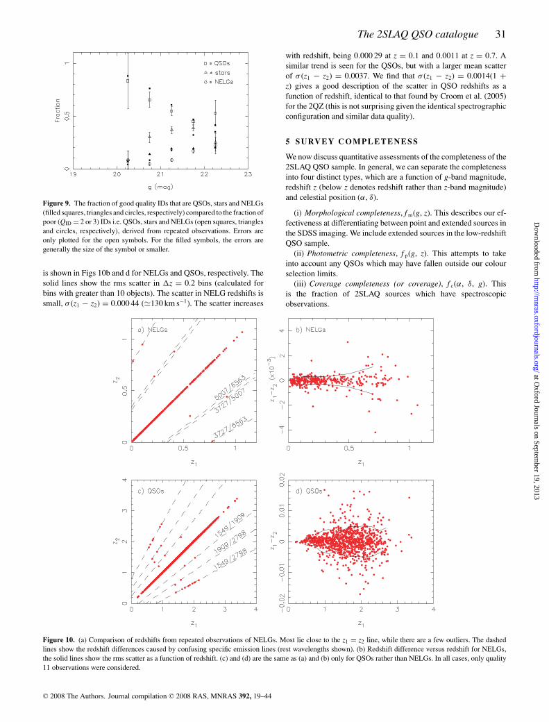
We assess the accuracy of our redshift estimates by examining thescatter in redshifts for repeated observations (quality 11 only); seeFig. 10. We do this separately for NELGs and QSOs, as the NELGswith their narrow lines have a much smaller dispersion than the
Table 9. The fraction of objects with the same ID which have differentredshifts in the different surveys (SDSS/2QZ/2SLAQ). 11-11 denotes aquality 11 spectrum for both the first and second catalogue listed in the firstcolumn; 11-12 denotes a quality 11 and a quality 12 spectrum for the firstand second catalogue listed etc.
Surveys QID Q Q Q Q1-1 11-11 11-12 12-11 12-12
SDSS–2QZ 3/512 2/510 1/2 0/0 0/0SDSS–2SLAQ 2/374 2/374 0/0 0/0 0/02QZ–2SLAQ 20/756 10/720 1/5 9/31 0/0
QSOs. Most repeated redshifts lie close to the line z1 = z2. However,a small number lie along lines denoting incorrect emission line IDs(dashed lines in Fig. 10). 7/385 NELGs (1.8 per cent) with repeatshave discrepant redshifts due to misidentification of emission lines.26/1032 QSO repeats (2.5 per cent) have discrepant redshifts, ofwhich half are due to confusion between Mg II and C IV. The scatterin redshift measurement after removing these catastrophic failures
C© 2008 The Authors. Journal compilation C© 2008 RAS, MNRAS 392, 19–44
at Oxford Journals on Septem
ber 19, 2013http://m
nras.oxfordjournals.org/D
ownloaded from
The 2SLAQ QSO catalogue 31
Figure 9. The fraction of good quality IDs that are QSOs, stars and NELGs(filled squares, triangles and circles, respectively) compared to the fraction ofpoor (QID = 2 or 3) IDs i.e. QSOs, stars and NELGs (open squares, trianglesand circles, respectively), derived from repeated observations. Errors areonly plotted for the open symbols. For the filled symbols, the errors aregenerally the size of the symbol or smaller.
is shown in Figs 10b and d for NELGs and QSOs, respectively. Thesolid lines show the rms scatter in �z = 0.2 bins (calculated forbins with greater than 10 objects). The scatter in NELG redshifts issmall, σ (z1 − z2) = 0.000 44 (�130 km s−1). The scatter increases
Figure 10. (a) Comparison of redshifts from repeated observations of NELGs. Most lie close to the z1 = z2 line, while there are a few outliers. The dashedlines show the redshift differences caused by confusing specific emission lines (rest wavelengths shown). (b) Redshift difference versus redshift for NELGs,the solid lines show the rms scatter as a function of redshift. (c) and (d) are the same as (a) and (b) only for QSOs rather than NELGs. In all cases, only quality11 observations were considered.
with redshift, being 0.000 29 at z = 0.1 and 0.0011 at z = 0.7. Asimilar trend is seen for the QSOs, but with a larger mean scatterof σ (z1 − z2) = 0.0037. We find that σ (z1 − z2) = 0.0014(1 +z) gives a good description of the scatter in QSO redshifts as afunction of redshift, identical to that found by Croom et al. (2005)for the 2QZ (this is not surprising given the identical spectrographicconfiguration and similar data quality).
5 SURVEY C OMPLETENESS
We now discuss quantitative assessments of the completeness of the2SLAQ QSO sample. In general, we can separate the completenessinto four distinct types, which are a function of g-band magnitude,redshift z (below z denotes redshift rather than z-band magnitude)and celestial position (α, δ).
(i) Morphological completeness, f m(g, z). This describes our ef-fectiveness at differentiating between point and extended sources inthe SDSS imaging. We include extended sources in the low-redshiftQSO sample.
(ii) Photometric completeness, f p(g, z). This attempts to takeinto account any QSOs which may have fallen outside our colourselection limits.
(iii) Coverage completeness (or coverage), f c(α, δ, g). Thisis the fraction of 2SLAQ sources which have spectroscopicobservations.
C© 2008 The Authors. Journal compilation C© 2008 RAS, MNRAS 392, 19–44
at Oxford Journals on Septem
ber 19, 2013http://m
nras.oxfordjournals.org/D
ownloaded from
32 S. M. Croom et al.
(iv) Spectroscopic completeness, f s(α, δ, g, z). This is the fractionof objects which have spectra with quality 1 IDs.
5.1 Morphological completeness
As discussed by R05, we initially included in our sample objectsthat the SDSS photometric pipeline (PHOTO; Lupton et al. 2001)classified as extended. This is because a significant number of pointsources are misclassified as extended at the faint limit of our sample(∼15 per cent; see fig. 5 of R05) and low-redshift QSOs can be gen-uinely extended. However, our first observing runs (2003 Marchand April) showed the sample contained large numbers of NELGs,of which many were extended. To reduce the contamination byNELGs, the final sample cuts were more restrictive and includedmorphology restrictions using the Bayesian star–galaxy classifier ofScranton et al. (2002). These are described, in detail, in Section 2.2.A total of 2144 objects were observed with the preliminary colourselection, of which 1021, 590, 283 and 250 were QSOs, NELGs,stars and ?? IDs, respectively. Of these sources, 284 were subse-quently rejected from the final catalogue on the basis of morphol-ogy, of which 262 were NELGs, nine QSOs, seven stars and sixunclassifiable. This morphological cut removed 44 per cent of theNELG contamination while only losing 0.9 per cent of the QSOs.The QSOs rejected by this cut are at low redshift, between z =0.12 and 0.84, and distributed uniformly within this interval. Thusat low redshift we do lose some QSOs due to the extended nature oftheir hosts. The seven stars rejected (all with g > 20.7) suggest thatat the faint limit the Bayesian star–galaxy classifier is not perfect,so that a small number of QSOs would be lost from the sample eventhough their true morphology was point like. Hence, the accuracy ofthe Bayesian star–galaxy classifier, together with our conservativecuts, means that the rejection of low-redshift QSOs is minimal, andwe will generally not correct for it in our analysis below.
As we incorporate 2QZ redshifts into the 2SLAQ catalogue, an-other issue to consider is that the 2QZ selection only included pointsources from Automated Plate Measurement (APM) scans of UnitedKingdom Schmidt Telescope (UKST) photographic plates. C04 andSmith et al. (2005) discuss the morphological selection of the 2QZin detail. There are two types of morphological incompleteness.The first is due to objects which are true point sources but whichthe APM software has classified as extended. From comparisonsto SDSS imaging data, Smith et al. (2005) show this to be a weakfunction of magnitude, rising from 6.4 per cent at the bright end and8.9 per cent at the faint end. Secondly, there are objects which aretruly extended (and classified as such from UKST plates), and there-fore missed by the 2QZ selection. C04 argue that this should onlybe a significant effect at z < 0.4 in the 2QZ given that the typicalsize of stellar images on UKST plates is 2–3 arcsec. In principle,the morphological bias of 2QZ objects could impact our 2SLAQcatalogue. This is because not all 2SLAQ selected targets have beenobserved spectroscopically, and those with 2QZ redshifts will pref-erentially be point sources. The vast majority of 2SLAQ sourceswith 2QZ spectra have g = 19.0 − 21.0; in this interval, the frac-tion of all QSOs which are classified as extended by SDSS (SDSStype = 3) was 10.3 ± 0.4 per cent. In contrast, 7.6 ± 0.6 per cent of2SLAQ QSOs which have 2QZ spectra are classified as extended.Therefore, 2.7 ± 0.7 per cent of QSOs may be missed if only tar-geted with 2QZ. Given the coverage completeness in the range∼70–80 per cent for the NGP (Fig. 4), the actual morpholog-ical bias introduced by the 2QZ selection will only be at the0.5–0.8 per cent level at worst. We therefore do not account forthis insignificant bias in our analysis below.
5.2 Photometric completeness
In order to determine the completeness of our sample, we constructa set of model QSO colours. In doing this, we aim to trace asaccurately as possible the underlying distribution, including theevolution of colour with redshift and a detailed consideration ofthe effects of host galaxies. These model colours are then passedthrough our selection algorithm to estimate the fraction of objectsselected. We use a modified version of the technique described byR05 (and Fan 1999), but unlike them, we also incorporate the impactof host galaxies.
5.2.1 Simulating QSO colours
We start by generating a set of QSO-only spectral energy distribu-tions (SEDs) (i.e. not including host-galaxy contributions) whichare well matched to the colours of bright (i < 18) SDSS QSOstaken from the DR3 catalogue (Schneider et al. 2005). These aresimilar to those generated by various other authors (e.g. Fan 1999;Richards et al. 2006). The underlying continuum is assumed to bea power law in frequency, ν, of the form fν ∝ ναν (equivalent to apower law in wavelength of fλ ∝ λ−[αν+2]). The power-law index,αν is normally distributed with a mean αν = −0.3 and a standarddeviation of 0.3. A mean of αν = −0.3 is slightly bluer than thatassumed by some other authors (e.g. Richards et al. (2006) used〈αν〉 = −0.5). We find that the bluer αν = −0.3, provides a bettermatch to the observed colours of bright QSOs. This may be becausethe measured redder slopes already include some contribution fromtheir host galaxy.
We then include an emission line component using the SDSSQSO composite (Vanden Berk et al. 2001). We divided the compos-ite spectrum by a fit to the continuum at λ < 5000 Å then subtracta second power-law redward of this limit. The composite is seen tohave a redder spectrum at λ > 5000 Å; probably due to contamina-tion of low-redshift QSOs by a host-galaxy contribution, which wewish to remove before creating our emission line spectrum. Hence,we subtract the continuum redward of this limit rather than divid-ing by it. All emission lines are assumed to have the same relativeequivalent width (EW), but the emission line spectrum is scaled bya factor that has a lognormal distribution with a mean of 1 and σ =0.48, consistent with the measurements made of the EW distribu-tion of 2QZ QSOs by Londish (2004). We also make a correction tothe flux around the Lyman-α line to account for absorption alreadypresent in the composite spectrum. To match the u − g colours ofQSOs at z ∼ 1.5–2.2 we boost the flux at λ = 1180–1290 Å by a fac-tor of 1.2. We add a Balmer continuum (BC) component to the QSOspectrum of the form given by equation (6) in Grandi (1982). Weuse a temperature of 12 000 K and the relative normalization of theBC component that is 0.05 of the underlying continuum at 3000 Å,which we find matches the observed colours of bright QSOs. Thisis somewhat lower than the 0.1 fraction used by Maddox & Hewett(2006) in their generation of simulated QSO spectra. We suspectthat this difference is due to the fact that the emission line spectrumwe use effectively contains some fraction of the BC component aswell.
Absorption bluewards of Lyman-α is added to the spectrum fol-lowing the recipe of Fan (1999) with some minor modifications.We calculate the contributions to the opacity for the first 10 transi-tions and use the accurate approximation of Tepper Garcıa (2006)to calculate Voigt profiles (although note that they have an errorin the equation in footnote 4 of their paper, and Q ≡ 1.5/x2 ratherthan Q ≡ 1.5x2). For each absorber, the Lyman limit absorption
C© 2008 The Authors. Journal compilation C© 2008 RAS, MNRAS 392, 19–44
at Oxford Journals on Septem
ber 19, 2013http://m
nras.oxfordjournals.org/D
ownloaded from
The 2SLAQ QSO catalogue 33
Table 10. Parameters of the assumed distribution of Lyman α forest, Lymanlimit and damped absorbers. The evolution of the absorbers is modelled bya power law of the form N(z) = N0(1 + z)γ and the H I column distributionis proportional to N−β
H . b is the Doppler width of the Voigt profile. Notethat these parameters are the same as those given by Fan (1999) with theexception of N0 for the Lyman α forest (Fan et al. used N0 = 50).
Absorption type log (NH) N0 γ β b(cm−2) (km s−1)
Lyman α forest 13.0–17.3 20.0 2.3 1.41 30Lyman limit 17.3–20.5 0.27 1.55 1.25 70
Damped Lyman α 20.5–22.0 0.04 1.3 1.48 70
was calculated using the prescription of Kennefick, Djorgovski &de Carvalho (1995). The forest, Lyman limit and damped absorbersare each distributed according to the values listed in Table 10, whichfollows closely the values listed by Fan (1999) except for the valueof N0 for the Lyman α forest. We find a better match to the QSOcolours with a lower value than Fan (1999).
Next, asinh magnitudes in the SDSS bands are calculated fromthe QSO SEDs, including the small corrections to transform fromtrue AB to the SDSS system (uAB = uSDSS + 0.04 and zAB = zSDSS +0.02) (Abazajian et al. 2004).
Finally, we add a Gaussian random error with a σ drawn from theSDSS PSF magnitude errors at the simulated magnitudes. This errorwas combined in quadrature with the uncertainties in the photomet-ric calibration (0.03 in u and z, and 0.02 in g, r and i). The colour–
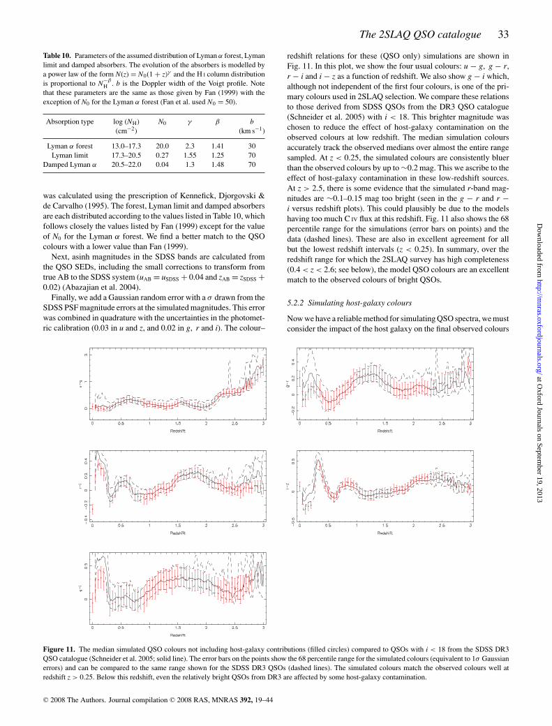
Figure 11. The median simulated QSO colours not including host-galaxy contributions (filled circles) compared to QSOs with i < 18 from the SDSS DR3QSO catalogue (Schneider et al. 2005; solid line). The error bars on the points show the 68 percentile range for the simulated colours (equivalent to 1σ Gaussianerrors) and can be compared to the same range shown for the SDSS DR3 QSOs (dashed lines). The simulated colours match the observed colours well atredshift z > 0.25. Below this redshift, even the relatively bright QSOs from DR3 are affected by some host-galaxy contamination.
redshift relations for these (QSO only) simulations are shown inFig. 11. In this plot, we show the four usual colours: u − g, g − r,r − i and i − z as a function of redshift. We also show g − i which,although not independent of the first four colours, is one of the pri-mary colours used in 2SLAQ selection. We compare these relationsto those derived from SDSS QSOs from the DR3 QSO catalogue(Schneider et al. 2005) with i < 18. This brighter magnitude waschosen to reduce the effect of host-galaxy contamination on theobserved colours at low redshift. The median simulation coloursaccurately track the observed medians over almost the entire rangesampled. At z < 0.25, the simulated colours are consistently bluerthan the observed colours by up to ∼0.2 mag. This we ascribe to theeffect of host-galaxy contamination in these low-redshift sources.At z > 2.5, there is some evidence that the simulated r-band mag-nitudes are ∼0.1–0.15 mag too bright (seen in the g − r and r −i versus redshift plots). This could plausibly be due to the modelshaving too much C IV flux at this redshift. Fig. 11 also shows the 68percentile range for the simulations (error bars on points) and thedata (dashed lines). These are also in excellent agreement for allbut the lowest redshift intervals (z < 0.25). In summary, over theredshift range for which the 2SLAQ survey has high completeness(0.4 < z < 2.6; see below), the model QSO colours are an excellentmatch to the observed colours of bright QSOs.
5.2.2 Simulating host-galaxy colours
Now we have a reliable method for simulating QSO spectra, we mustconsider the impact of the host galaxy on the final observed colours
C© 2008 The Authors. Journal compilation C© 2008 RAS, MNRAS 392, 19–44
at Oxford Journals on Septem
ber 19, 2013http://m
nras.oxfordjournals.org/D
ownloaded from
34 S. M. Croom et al.
of 2SLAQ objects. The 2SLAQ selection is based on SDSS PSFphotometry, so host-galaxy contributions are to some extent mini-mized, but at the faint flux limits we reach these PSF magnitudesstill contain significant host-galaxy contributions (e.g. Schneideret al. 2003). We start by considering the observed relation betweenLQSO and Lgal from the low-redshift host-galaxy analysis of Schade,Boyle & Letawsky (2000). Taking this data and fitting a relation
Mgal = A + BMQSO (7)
to all objects with point source detections in the B band brighterthan MB (AB) = −16, we obtain A = −17.1 ± 1.1 and B =0.21 ± 0.05 with a scatter, σ qg = 0.7 in Mgal. If we, instead, assumeno correlation between Mgal and MQSO, we find the mean Mgal(AB)is −21.3 with an rms scatter of 0.8. Within the luminosity rangethat Schade et al. probe, the Mgal–MQSO correlation is significant,but if brighter AGN are added to the sample, the relation appears toflatten (see fig. 13c of Schade et al.). With this in mind, below wewill investigate whether we can constrain the slope of the relationby comparing our simulations and 2SLAQ colours.
Our approach is to constrain as many parameters of the host-galaxy SED as possible from independent observations and thenuse the colour distribution of the 2SLAQ QSOs to adjust the otherparameters. In particular, we need to ensure that when we apply thecolour-selection criteria to our simulated QSOs that we obtain thesame colour distribution as for the real data. This is a necessary,but not sufficient, requirement to demonstrate that our simulationsaccurately model the colours of the underlying population.
Broad-band colours alone, especially when combined with a QSOSED, are not adequate to fully constrain the host-galaxy SEDs. Wetherefore consider a number of possible star formation scenariosand model SEDs using the Bruzual & Charlot (2003) populationsynthesis code. We assume a solar metallicity and Chabrier (2003)initial mass function (IMF) for all models, on the basis that high-redshift QSO metallicities are typically found to be high (Dietrichet al. 2003; Kurk et al. 2007), and that with only a small numberof broad-band colours we cannot hope to separate out the effects ofany metallicity or IMF variation.
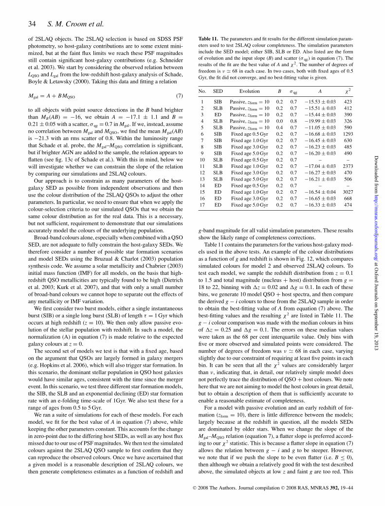
We first consider two burst models, either a single instantaneousburst (SIB) or a single long burst (SLB) of length τ = 1 Gyr whichoccurs at high redshift (z = 10). We then only allow passive evo-lution of the stellar population with redshift. In such a model, thenormalization (A) in equation (7) is made relative to the expectedgalaxy colours at z = 0.
The second set of models we test is that with a fixed age, basedon the argument that QSOs are largely formed in galaxy mergers(e.g. Hopkins et al. 2006), which will also trigger star formation. Inthis scenario, the dominant stellar population in QSO host galaxieswould have similar ages, consistent with the time since the mergerevent. In this scenario, we test three different star formation models,the SIB, the SLB and an exponential declining (ED) star formationrate with an e-folding time-scale of 1Gyr. We also test these for arange of ages from 0.5 to 5 Gyr.
We ran a suite of simulations for each of these models. For eachmodel, we fit for the best value of A in equation (7) above, whilekeeping the other parameters constant. This accounts for the changein zero-point due to the differing host SEDs, as well as any host fluxmissed due to our use of PSF magnitudes. We then test the simulatedcolours against the 2SLAQ QSO sample to first confirm that theycan reproduce the observed colours. Once we have ascertained thata given model is a reasonable description of 2SLAQ colours, wethen generate completeness estimates as a function of redshift and
Table 11. The parameters and fit results for the different simulation param-eters used to test 2SLAQ colour completeness. The simulation parametersinclude the SED model; either SIB, SLB or ED. Also listed are the formof evolution and the input slope (B) and scatter (σ qg) in equation (7). Theresults of the fit are the best value of A and χ2. The number of degrees offreedom is ν � 68 in each case. In two cases, both with fixed ages of 0.5Gyr, the fit did not converge, and no best-fitting value is given.
No. SED Evolution B σ qg A χ2
1 SIB Passive, zform = 10 0.2 0.7 −15.53 ± 0.03 4232 SLB Passive, zform = 10 0.2 0.7 −15.51 ± 0.03 4123 ED Passive, zform = 10 0.2 0.7 −15.44 ± 0.03 3904 SLB Passive, zform = 10 0.0 0.8 −19.99 ± 0.03 3265 SLB Passive, zform = 10 0.4 0.7 −11.05 ± 0.03 5906 SIB Fixed age 0.5 Gyr 0.2 0.7 −16.68 ± 0.03 12937 SIB Fixed age 1.0 Gyr 0.2 0.7 −16.45 ± 0.03 6308 SIB Fixed age 3.0 Gyr 0.2 0.7 −16.23 ± 0.03 4859 SIB Fixed age 5.0 Gyr 0.2 0.7 −16.20 ± 0.03 490
10 SLB Fixed age 0.5 Gyr 0.2 0.7 – –11 SLB Fixed age 1.0 Gyr 0.2 0.7 −17.04 ± 0.03 237312 SLB Fixed age 3.0 Gyr 0.2 0.7 −16.27 ± 0.03 47013 SLB Fixed age 5.0 Gyr 0.2 0.7 −16.21 ± 0.03 50614 ED Fixed age 0.5 Gyr 0.2 0.7 – –15 ED Fixed age 1.0 Gyr 0.2 0.7 −16.54 ± 0.04 302716 ED Fixed age 3.0 Gyr 0.2 0.7 −16.65 ± 0.03 66817 ED Fixed age 5.0 Gyr 0.2 0.7 −16.33 ± 0.03 474
g-band magnitude for all valid simulation parameters. These resultsshow the likely range of completeness corrections.
Table 11 contains the parameters for the various host-galaxy mod-els used in the above tests. An example of the colour distributionsas a function of g and redshift is shown in Fig. 12, which comparessimulated colours for model 2 and observed 2SLAQ colours. Totest each model, we sample the redshift distribution from z = 0.1to 1.5 and total magnitude (nucleus + host) distribution from g =18 to 22, binning with �z = 0.02 and �g = 0.1. In each of thesebins, we generate 10 model QSO + host spectra, and then comparethe derived g − i colours to those from the 2SLAQ sample in orderto obtain the best-fitting value of A from equation (7) above. Thebest-fitting values and the resulting χ 2 are listed in Table 11. Theg − i colour comparison was made with the median colours in binsof �z = 0.25 and �g = 0.1. The errors on these median valueswere taken as the 68 per cent interquartile value. Only bins withfive or more observed and simulated points were considered. Thenumber of degrees of freedom was ν � 68 in each case, varyingslightly due to our constraint of requiring at least five points in eachbin. It can be seen that all the χ 2 values are considerably largerthan ν, indicating that, in detail, our relatively simple model doesnot perfectly trace the distribution of QSO + host colours. We notehere that we are not aiming to model the host colours in great detail,but to obtain a description of them that is sufficiently accurate toenable a reasonable estimate of completeness.
For a model with passive evolution and an early redshift of for-mation (zform = 10), there is little difference between the models;largely because at the redshift in question, all the models SEDsare dominated by older stars. When we change the slope of theMgal–MQSO relation (equation 7), a flatter slope is preferred accord-ing to our χ 2 statistic. This is because a flatter slope in equation (7)allows the relation between g − i and g to be steeper. However,we note that if we push the slope to be even flatter (i.e. B ≤ 0),then although we obtain a relatively good fit with the test describedabove, the simulated objects at low z and faint g are too red. This
C© 2008 The Authors. Journal compilation C© 2008 RAS, MNRAS 392, 19–44
at Oxford Journals on Septem
ber 19, 2013http://m
nras.oxfordjournals.org/D
ownloaded from
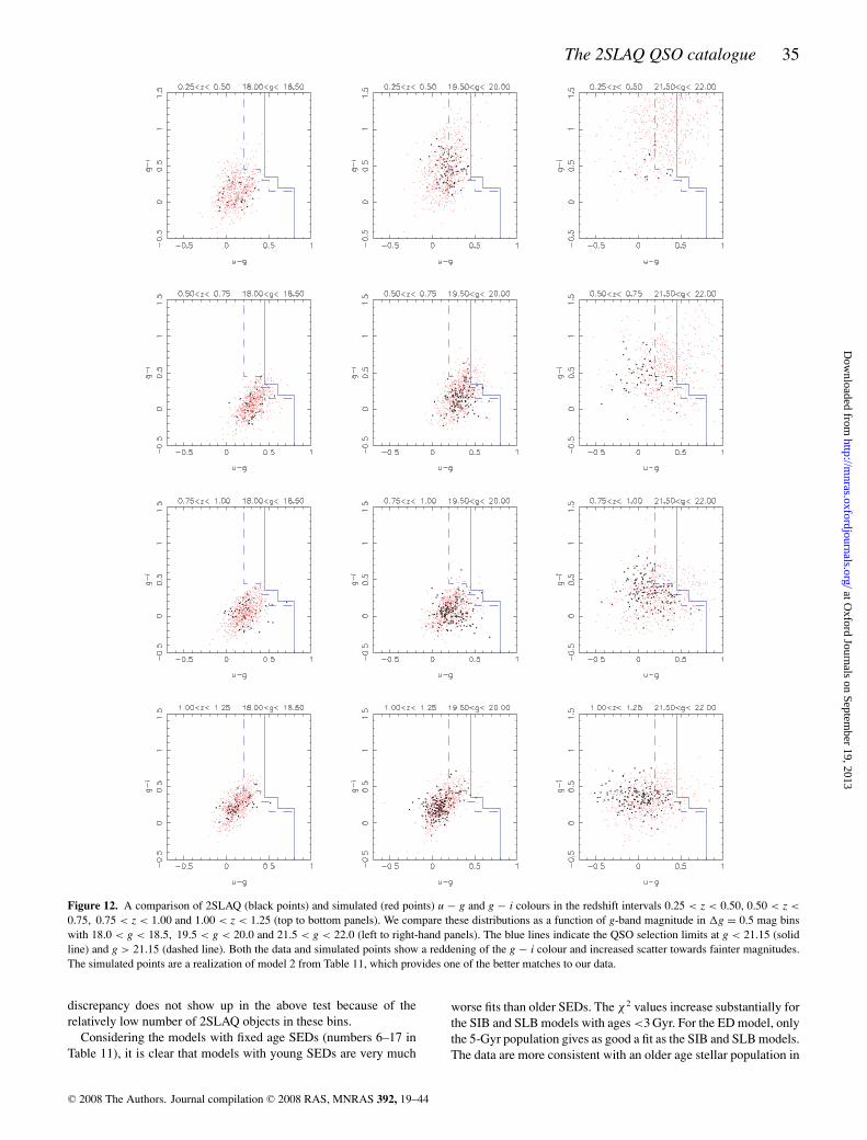
The 2SLAQ QSO catalogue 35
Figure 12. A comparison of 2SLAQ (black points) and simulated (red points) u − g and g − i colours in the redshift intervals 0.25 < z < 0.50, 0.50 < z <
0.75, 0.75 < z < 1.00 and 1.00 < z < 1.25 (top to bottom panels). We compare these distributions as a function of g-band magnitude in �g = 0.5 mag binswith 18.0 < g < 18.5, 19.5 < g < 20.0 and 21.5 < g < 22.0 (left to right-hand panels). The blue lines indicate the QSO selection limits at g < 21.15 (solidline) and g > 21.15 (dashed line). Both the data and simulated points show a reddening of the g − i colour and increased scatter towards fainter magnitudes.The simulated points are a realization of model 2 from Table 11, which provides one of the better matches to our data.
discrepancy does not show up in the above test because of therelatively low number of 2SLAQ objects in these bins.
Considering the models with fixed age SEDs (numbers 6–17 inTable 11), it is clear that models with young SEDs are very much
worse fits than older SEDs. The χ 2 values increase substantially forthe SIB and SLB models with ages <3 Gyr. For the ED model, onlythe 5-Gyr population gives as good a fit as the SIB and SLB models.The data are more consistent with an older age stellar population in
C© 2008 The Authors. Journal compilation C© 2008 RAS, MNRAS 392, 19–44
at Oxford Journals on Septem
ber 19, 2013http://m
nras.oxfordjournals.org/D
ownloaded from

36 S. M. Croom et al.
the host galaxies because of the red colours of faint 2SLAQ objectsin g − i. This can be seen in Fig 12, which shows the reddening of∼0.5 mag in g − i from g = 18.0 to 22.0, in the redshift interval0.50 < z < 0.75. A significant young and blue (<1 Gyr) stellarpopulation is inconsistent with the observed trend, as reflected inthe poorer χ 2 fits in Table 11. This could provide challenges formodels of QSO formation which rely on mergers to trigger QSOactivity and star formation (Hopkins et al. 2006), as it implies thatthe dominant stellar population is relatively old. However, giventhat the objects in question are at low redshift and low luminosity, itcould be that major mergers do not play such a significant role forthis faint population (Hopkins & Hernquist 2006). Indeed, variousobservations of more luminous QSO have found evidence that thehosts are bluer than typical galaxies, with relatively young stellarpopulations (e.g. Kirhakos et al. 1999; Zakamska et al. 2006). Atlow redshift (z < 0.3), Kauffmann et al. (2003) show that the stellarpopulations in the host galaxies of type II AGN are similar to non-active early-type galaxies, although at high luminosity the stellarpopulation becomes younger [as measured by the Dn(4000) index].Vanden Berk et al. (2006) find that hosts of SDSS quasars at z < 0.75span a wide range of spectral types, but at low host (and nuclear)luminosity the typical colours are similar to non-active early types.Our estimates of host galaxies properties seem broadly consistentwith this work.
The final step is to compare the completeness estimates fromthe different models in order to determine the uncertainty in ourcompleteness corrections. We simulate the redshift range 0.1 <
z < 3.0 and use 18 < g < 22. We use the bins �z = 0.02 and�g = 0.1 and increase the number of simulated objects to 200 perbin, so that our completeness estimates are not limited by shot noise.We find that the largest variation in estimated completeness from
Figure 13. A comparison of photometric completeness as a function of redshift for four different apparent magnitude slices with mean g-band magnitude (a)g = 18.525, (b) g = 19.525, (c) g = 20.525 and (d) g = 21.525. We compare models with different values of B (defined in equation 7), B = 0.0 (dashed redline), B = 0.2 (solid black line) and B = 0.4 (dotted blue line) which are models 4, 2 and 5, respectively in Table 11. At bright magnitudes and/or high redshift,all three models agree very well, while at faint magnitudes the models diverge below z ∼ 0.5.
within our suite of models is due to the variation in the parameterB in equation (7). In Fig. 13, we plot models 2, 4 and 5 fromTable 11 for four different g-band magnitude slices. It is only atfaint magnitudes and redshifts less than ∼0.5 that the completenessdepends on the model. To quantify this further, Fig. 14 plots themean fractional difference in the models, i.e. 0.5(C4 − C5)/C2,where C2 is the completeness in model 2 etc. We overlay contoursof constant absolute g-band magnitude (blue lines) from Mg =−24 (top panel) to −20 (bottom panel) (using the Cristiani & Vio1990 K-correction). Brighter than Mg � −21, the uncertainty on thecompleteness estimate is less than 20 per cent and by Mg � −21.5this uncertainty is less than 5 per cent.
Based on this, we adopt model 2 for our final colour completeness.This provides a reasonable match to the observed 2SLAQ QSOcolours as well as being midway between the models with thelargest variations (i.e. models 4 and 5). The completeness array forthis model is shown in Fig. 15. The step at g = 21.15, where wechange our colour selection limits, is clearly visible. In contrastto our previous estimates of the completeness of 2SLAQ selection(see R05), the completeness derived here declines much more atfaint magnitudes and low redshift. Table 12 contains the colourcompleteness array as a function of z and g. The full table is availablein the electronic version of the journal.
5.2.3 Correcting for host-galaxy flux
Our detailed simulations enable a relatively straightforward mech-anism to correct the photometry of the 2SLAQ QSOs for the con-tribution of their host galaxy. The photometry used to select targetsand calculate luminosities was based on SDSS PSF magnitudes, sothis should limit the contribution of the host to some extent, but
C© 2008 The Authors. Journal compilation C© 2008 RAS, MNRAS 392, 19–44
at Oxford Journals on Septem
ber 19, 2013http://m
nras.oxfordjournals.org/D
ownloaded from

The 2SLAQ QSO catalogue 37
Figure 14. The fractional difference between completeness estimates as-suming host-galaxy models 2, 4 and 5. We plot 0.5(C4 − C5)/C2 where C4
is the completeness in model 4 etc. The contours are at 0.1 intervals (0.1,0.3 . . . dashed red lines; 0.2, 0.4 . . . solid red lines), and the same data arealso plotted as a grey scale. The solid blue lines denote lines of constant ab-solute magnitude from Mg = −24 (top panel) to Mg = −20 (bottom panel)in 1.0 mag intervals. At Mg = −21, the uncertainty in the completeness isalways less than 20 per cent. Note the more limited redshift range comparedto Fig. 15 below.
Figure 15. The final photometric completeness map for the 2SLAQ sampleas a function of g and z assuming model 2. The contours are at 0.1 intervals(0.1, 0.3 . . . dashed red lines; 0.2, 0.4 . . . solid red lines), and the same dataare also plotted as a grey scale. The solid blue lines denote lines of constantabsolute magnitude from Mg = −24 (top panel) to Mg = −20 (bottompanel) in 1.0 mag intervals.
up to z � 1 there is some contribution from the host in the PSFmagnitudes. For each simulated source, we calculate the total PSFmagnitude (mtot, QSO + host) and the difference between total andthe QSO, mQSO − mtot. We can then derive the mean correction fromtotal to nuclear magnitude in the same g-band and redshift intervalsused to make the completeness correction array. Fig. 16 shows thefractional host contribution to the PSF flux in the g (top panel) andi (bottom panel) bands. In the g-band, which forms the flux limit ofthe 2SLAQ sample, the host contribution is less than 20 per cent atz > 0.4, even for the faintest sources. However, it is not until z ∼0.9 that the contribution falls below 20 per cent in the i-band. Thesecorrections can be applied to determine nuclear fluxes for 2SLAQsources. The host-galaxy contributions as a function of redshift andg- and i-band magnitude are listed in Table 12.
Table 12. The 2SLAQ colour completeness array. The completeness isgiven as a function of redshift, z, and g-band magnitude. We also list thehost-galaxy contribution as a magnitude difference, �host, in both the g andi bands. The first 10 rows are given here. The full table is available in theelectronic version of the journal.
z Mag. Completeness �host �hostg/i g (mag) i (mag)
0.200 18.275 0.92 0.19 0.810.200 18.525 0.85 0.23 0.990.200 18.775 0.79 0.27 1.110.200 19.025 0.69 0.31 1.260.200 19.275 0.62 0.36 1.410.200 19.525 0.52 0.40 1.550.200 19.775 0.40 0.46 1.730.200 20.025 0.31 0.53 1.910.200 20.275 0.23 0.60 2.100.200 20.525 0.14 0.68 2.29
Figure 16. Top panel: the fractional contribution of the host galaxy tothe total g-band PSF flux of 2SLAQ QSOs as a function of g and z (as-suming model 2 from Table 11). The contours are at 0.05 intervals (0.05,0.15 . . . dashed red lines; 0.1, 0.2 . . . solid red lines), and the data are alsoplotted as a grey scale. The solid blue lines denote lines of constant absolutemagnitude from Mg = −24 (top panel) to Mg = −20 (bottom panel) in1.0 mag intervals. Bottom panel: same as above, but showing the fractionalcontribution of the host galaxy to the total i-band PSF flux as a function ofredshift and i-band flux. At low redshift and faint i-band flux, these i-bandhost contributions are extrapolated from the comparison to the 2SLAQ data.This is because the combined QSO + host colours are relatively red, g −i ∼ 1, so that a source with i � 22 will be ∼1 mag fainter than the 2SLAQg-band limit.
C© 2008 The Authors. Journal compilation C© 2008 RAS, MNRAS 392, 19–44
at Oxford Journals on Septem
ber 19, 2013http://m
nras.oxfordjournals.org/D
ownloaded from
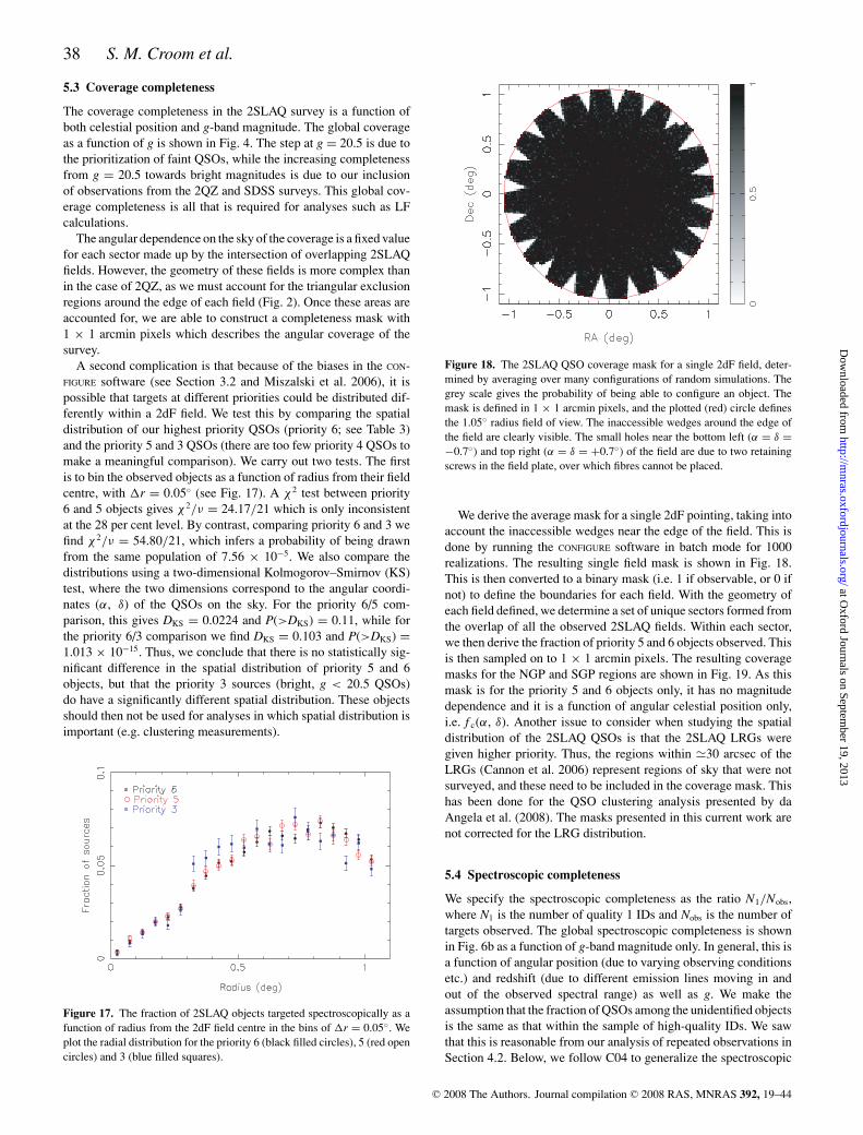
38 S. M. Croom et al.
5.3 Coverage completeness
The coverage completeness in the 2SLAQ survey is a function ofboth celestial position and g-band magnitude. The global coverageas a function of g is shown in Fig. 4. The step at g = 20.5 is due tothe prioritization of faint QSOs, while the increasing completenessfrom g = 20.5 towards bright magnitudes is due to our inclusionof observations from the 2QZ and SDSS surveys. This global cov-erage completeness is all that is required for analyses such as LFcalculations.
The angular dependence on the sky of the coverage is a fixed valuefor each sector made up by the intersection of overlapping 2SLAQfields. However, the geometry of these fields is more complex thanin the case of 2QZ, as we must account for the triangular exclusionregions around the edge of each field (Fig. 2). Once these areas areaccounted for, we are able to construct a completeness mask with1 × 1 arcmin pixels which describes the angular coverage of thesurvey.
A second complication is that because of the biases in the CON-FIGURE software (see Section 3.2 and Miszalski et al. 2006), it ispossible that targets at different priorities could be distributed dif-ferently within a 2dF field. We test this by comparing the spatialdistribution of our highest priority QSOs (priority 6; see Table 3)and the priority 5 and 3 QSOs (there are too few priority 4 QSOs tomake a meaningful comparison). We carry out two tests. The firstis to bin the observed objects as a function of radius from their fieldcentre, with �r = 0.05◦ (see Fig. 17). A χ 2 test between priority6 and 5 objects gives χ 2/ν = 24.17/21 which is only inconsistentat the 28 per cent level. By contrast, comparing priority 6 and 3 wefind χ 2/ν = 54.80/21, which infers a probability of being drawnfrom the same population of 7.56 × 10⁻⁵. We also compare thedistributions using a two-dimensional Kolmogorov–Smirnov (KS)test, where the two dimensions correspond to the angular coordi-nates (α, δ) of the QSOs on the sky. For the priority 6/5 com-parison, this gives DKS = 0.0224 and P(>DKS) = 0.11, while forthe priority 6/3 comparison we find DKS = 0.103 and P(>DKS) =1.013 × 10⁻¹⁵. Thus, we conclude that there is no statistically sig-nificant difference in the spatial distribution of priority 5 and 6objects, but that the priority 3 sources (bright, g < 20.5 QSOs)do have a significantly different spatial distribution. These objectsshould then not be used for analyses in which spatial distribution isimportant (e.g. clustering measurements).
Figure 17. The fraction of 2SLAQ objects targeted spectroscopically as afunction of radius from the 2dF field centre in the bins of �r = 0.05◦. Weplot the radial distribution for the priority 6 (black filled circles), 5 (red opencircles) and 3 (blue filled squares).
Figure 18. The 2SLAQ QSO coverage mask for a single 2dF field, deter-mined by averaging over many configurations of random simulations. Thegrey scale gives the probability of being able to configure an object. Themask is defined in 1 × 1 arcmin pixels, and the plotted (red) circle definesthe 1.05◦ radius field of view. The inaccessible wedges around the edge ofthe field are clearly visible. The small holes near the bottom left (α = δ =−0.7◦) and top right (α = δ = +0.7◦) of the field are due to two retainingscrews in the field plate, over which fibres cannot be placed.
We derive the average mask for a single 2dF pointing, taking intoaccount the inaccessible wedges near the edge of the field. This isdone by running the CONFIGURE software in batch mode for 1000realizations. The resulting single field mask is shown in Fig. 18.This is then converted to a binary mask (i.e. 1 if observable, or 0 ifnot) to define the boundaries for each field. With the geometry ofeach field defined, we determine a set of unique sectors formed fromthe overlap of all the observed 2SLAQ fields. Within each sector,we then derive the fraction of priority 5 and 6 objects observed. Thisis then sampled on to 1 × 1 arcmin pixels. The resulting coveragemasks for the NGP and SGP regions are shown in Fig. 19. As thismask is for the priority 5 and 6 objects only, it has no magnitudedependence and it is a function of angular celestial position only,i.e. f c(α, δ). Another issue to consider when studying the spatialdistribution of the 2SLAQ QSOs is that the 2SLAQ LRGs weregiven higher priority. Thus, the regions within �30 arcsec of theLRGs (Cannon et al. 2006) represent regions of sky that were notsurveyed, and these need to be included in the coverage mask. Thishas been done for the QSO clustering analysis presented by daAngela et al. (2008). The masks presented in this current work arenot corrected for the LRG distribution.
5.4 Spectroscopic completeness
We specify the spectroscopic completeness as the ratio N1/Nobs,where N1 is the number of quality 1 IDs and Nobs is the number oftargets observed. The global spectroscopic completeness is shownin Fig. 6b as a function of g-band magnitude only. In general, this isa function of angular position (due to varying observing conditionsetc.) and redshift (due to different emission lines moving in andout of the observed spectral range) as well as g. We make theassumption that the fraction of QSOs among the unidentified objectsis the same as that within the sample of high-quality IDs. We sawthat this is reasonable from our analysis of repeated observations inSection 4.2. Below, we follow C04 to generalize the spectroscopic
C© 2008 The Authors. Journal compilation C© 2008 RAS, MNRAS 392, 19–44
at Oxford Journals on Septem
ber 19, 2013http://m
nras.oxfordjournals.org/D
ownloaded from
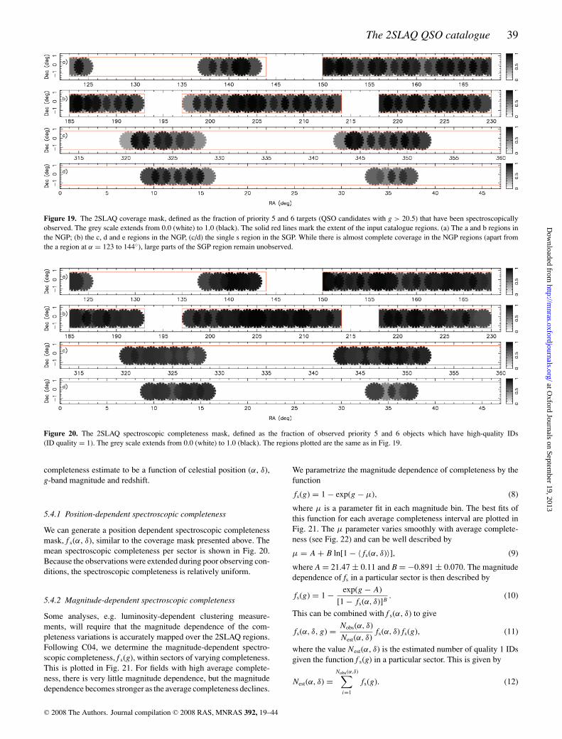
The 2SLAQ QSO catalogue 39
Figure 19. The 2SLAQ coverage mask, defined as the fraction of priority 5 and 6 targets (QSO candidates with g > 20.5) that have been spectroscopicallyobserved. The grey scale extends from 0.0 (white) to 1.0 (black). The solid red lines mark the extent of the input catalogue regions. (a) The a and b regions inthe NGP; (b) the c, d and e regions in the NGP, (c/d) the single s region in the SGP. While there is almost complete coverage in the NGP regions (apart fromthe a region at α = 123 to 144◦), large parts of the SGP region remain unobserved.
Figure 20. The 2SLAQ spectroscopic completeness mask, defined as the fraction of observed priority 5 and 6 objects which have high-quality IDs(ID quality = 1). The grey scale extends from 0.0 (white) to 1.0 (black). The regions plotted are the same as in Fig. 19.
completeness estimate to be a function of celestial position (α, δ),g-band magnitude and redshift.
5.4.1 Position-dependent spectroscopic completeness
We can generate a position dependent spectroscopic completenessmask, f s(α, δ), similar to the coverage mask presented above. Themean spectroscopic completeness per sector is shown in Fig. 20.Because the observations were extended during poor observing con-ditions, the spectroscopic completeness is relatively uniform.
5.4.2 Magnitude-dependent spectroscopic completeness
Some analyses, e.g. luminosity-dependent clustering measure-ments, will require that the magnitude dependence of the com-pleteness variations is accurately mapped over the 2SLAQ regions.Following C04, we determine the magnitude-dependent spectro-scopic completeness, f s(g), within sectors of varying completeness.This is plotted in Fig. 21. For fields with high average complete-ness, there is very little magnitude dependence, but the magnitudedependence becomes stronger as the average completeness declines.
We parametrize the magnitude dependence of completeness by thefunction
fs(g) = 1 − exp(g − μ), (8)
where μ is a parameter fit in each magnitude bin. The best fits ofthis function for each average completeness interval are plotted inFig. 21. The μ parameter varies smoothly with average complete-ness (see Fig. 22) and can be well described by
μ = A + B ln[1 − 〈fs(α, δ)〉], (9)
where A = 21.47 ± 0.11 and B = −0.891 ± 0.070. The magnitudedependence of fs in a particular sector is then described by
fs(g) = 1 − exp(g − A)
[1 − fs(α, δ)]B. (10)
This can be combined with f s(α, δ) to give
fs(α, δ, g) = Nobs(α, δ)
Nest(α, δ)fs(α, δ)fs(g), (11)
where the value Nest(α, δ) is the estimated number of quality 1 IDsgiven the function f s(g) in a particular sector. This is given by
Nest(α, δ) =Nobs(α,δ)∑
i=1
fs(g). (12)
C© 2008 The Authors. Journal compilation C© 2008 RAS, MNRAS 392, 19–44
at Oxford Journals on Septem
ber 19, 2013http://m
nras.oxfordjournals.org/D
ownloaded from
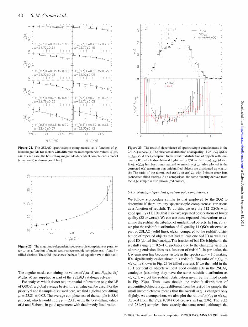
40 S. M. Croom et al.
Figure 21. The 2SLAQ spectroscopic completeness as a function of g-band magnitude for sectors with different mean completeness values, 〈f s(α,δ)〉. In each case, the best-fitting magnitude-dependent completeness model(equation 8) is shown (solid line).
Figure 22. The magnitude-dependent spectroscopic completeness parame-ter, μ, as a function of mean sector spectroscopic completeness, 〈f s(α, δ)〉(filled circles). The solid line shows the best fit of equation (9) to this data.
The angular masks containing the values of f s(α, δ) and Nobs(α, δ)/Nest(α, δ) are supplied as part of the 2SLAQ catalogue release.
For analyses which do not require spatial information (e.g. the LFof QSOs), a global average best-fitting μ value can be used. For thepriority 5 and 6 sample discussed here, we find a global best-fittingμ = 23.21 ± 0.03. The average completeness of the sample is 85.4per cent, which would imply μ = 23.18 using the best-fitting valuesof A and B above, in good agreement with the directly fitted value.
Figure 23. The redshift dependence of spectroscopic completeness in the2SLAQ survey. (a) The observed distribution of all quality 11 2SLAQ QSOs,n(z)all (solid line), compared to the redshift distribution of objects with low-quality IDs which also obtained high-quality QSO redshifts, n(z)bad (dottedline). n(z)all has been renormalized to match n(z)bad. Also plotted is thecorrected n(z) assuming that unidentified objects are distributed as n(z)bad.(b) The ratio of the normalized n(z)all to n(z)bad with Poisson error bars(connected filled circles). As a comparison, the same quantity derived fromthe 2QZ sample is also shown (red crosses).
5.4.3 Redshift-dependent spectroscopic completeness
We follow a procedure similar to that employed by the 2QZ todetermine if there are any spectroscopic completeness variationsas a function of redshift. To do this, we use the 512 QSOs withgood quality (11) IDs, that also have repeated observations of lowerquality (22 or worse). We can use these repeated observations to ex-amine the redshift distribution of unidentified objects. In Fig. 23(a),we plot the redshift distribution of all quality 11 QSOs observed aspart of 2SLAQ (solid line), n(z)all, compared to the redshift distri-bution of repeated objects that had at least one bad ID as well as agood ID (dotted line), n(z)bad. The fraction of bad IDs is higher in theredshift range z � 0.5–1.6, probably due to the changing visibilityof strong emission lines as a function of redshift. In particular, theC IV emission line becomes visible in the spectra at z ∼ 1.5 makingIDs significantly easier above this redshift. The ratio of n(z)all ton(z)bad is shown in Fig. 23(b) (filled circles). If we then add in the13.1 per cent of objects without good quality IDs in the 2SLAQcatalogue [assuming they have the same redshift distribution asn(z)bad], we get the redshift distribution given by the filled pointsin Fig. 23(a). Thus, even though the redshift distribution ofunidentified objects is quite different from the rest of the sample, thesmall incompleteness means that the overall n(z) is changed onlyslightly. As a comparison, we also plot the ratio of n(z)all to n(z)bad
derived from the 2QZ (C04) (red crosses in Fig. 23b). The 2QZand 2SLAQ samples show exactly the same trends, although the
C© 2008 The Authors. Journal compilation C© 2008 RAS, MNRAS 392, 19–44
at Oxford Journals on Septem
ber 19, 2013http://m
nras.oxfordjournals.org/D
ownloaded from

The 2SLAQ QSO catalogue 41
Table 13. Derived values for R(z) ≡ n(z)all/n(z)bad [and errors, σR(z)] thatcan be used to estimate the redshift dependence of spectroscopic incom-pleteness. Data are binned in �z = 0.1 bins.
z R(z) σR(z) z R(z) σR(z)
0.15 0.72 0.75 1.55 0.74 0.120.25 0.78 0.57 1.65 1.15 0.240.35 4.13 4.16 1.75 1.15 0.220.45 1.46 0.67 1.85 1.14 0.220.55 1.05 0.36 1.95 1.24 0.270.65 1.00 0.29 2.05 1.44 0.340.75 0.67 0.13 2.15 1.62 0.420.85 1.17 0.27 2.25 1.75 0.560.95 0.58 0.10 2.35 2.31 0.961.05 0.78 0.14 2.45 2.18 0.901.15 0.65 0.10 2.55 4.48 3.191.25 0.78 0.14 2.65 6.10 6.131.35 0.69 0.11 2.75 2.81 2.841.45 0.76 0.13
amplitude of the variations is somewhat higher for the 2SLAQ sam-ple. This could be due to the Baldwin (1977) effect, which causesemission lines to be stronger in lower luminosity QSOs.
Following the procedure used for the 2QZ, we define a functionR(z) such that
R(z) = n(z)all
n(z)bad, (13)
where both n(z)all and n(z)bad are normalized such that the sumof all redshift bins is equal to one. This is the value plotted inFig. 23(b) and also tabulated in Table 13. The angular and magnitudedependent completeness is then given by
fs(α, δ, g, z) ={
1 + 1
R(z)
[1
fs(α, δ, g)− 1
]}−1
. (14)
This relation can then be used to describe the variations in com-pleteness in a general sense for the 2SLAQ sample. We note thatin this analysis we have assumed that the redshift dependence isseparable from f s(α, δ, g). That is, we have assumed that the formof R(z) does not depend on angular position or g-band magnitude.
6 SU M M A RY
In this paper, we present the spectroscopic QSO catalogue fromthe 2SLAQ survey. This sample is flux limited at 18 < g < 21.85(extinction corrected), and covers an area of 191.9 deg2. We havetaken new spectra of 16326 objects, of which 8764 are QSOs. Ofthese, 7623 are newly discovered (the remainder were previouslyidentified by the 2QZ and SDSS surveys). The full QSO sample (in-cluding objects previously observed in the SDSS and 2QZ surveys)contains 12702 QSOs.
We present detailed completeness estimates for the survey, basedon modelling of QSO colours, including host-galaxy contributions.This calculation shows that at g � 21.85 QSO colours are signifi-cantly affected by the presence of a host galaxy up to z ∼ 1 in theSDSS ugriz bands. In particular, we see a significant reddening ofthe objects in g − i towards fainter g-band magnitudes. This impliesthat the host galaxies of these faint 2SLAQ QSOs are dominatedby an old (�2–3Gyr) stellar population and not a young starburstcomponent.
The primary aim of the 2SLAQ QSO sample is to study the lumi-nosity and spatial distribution of QSOs beyond the observed break
in the QSO LF. In this context, it is particularly important that de-tailed corrections for completeness (including host-galaxy effects)are carried out. If we can learn how to account for the contami-nation in optical samples, new larger area optical imaging surveys(e.g. LSST; Ivezic et al. 2008) will allow substantial improvementsin our characterization of the evolution of AGN.
The LF from the final 2SLAQ catalogue is presented in a com-panion paper (Croom et al. in preparation). The 2SLAQ QSO cata-logue, along with completeness estimates, is publically available athttp://www.2slaq.info/.
AC K N OW L E D G M E N T S
The 2SLAQ survey is based on the observations carried out with theAAT and as a part of the SDSS. We warmly thank all the present andformer staff of the Anglo-Australian Observatory for their work inbuilding and operating the 2dF facility. The 2QZ survey is based onthe observations made with the AAT and the UK Schmidt Telescope.
Funding for the SDSS and SDSS II has been provided by theAlfred P. Sloan Foundation, the Participating Institutions, the Na-tional Science Foundation, the US Department of Energy, theNational Aeronautics and Space Administration, the JapaneseMonbukagakusho, the Max Planck Society and the Higher Ed-ucation Funding Council for England. The SDSS Web Site ishttp://www.sdss.org/.
The SDSS is managed by the Astrophysical Research Consor-tium for the Participating Institutions. The Participating Institu-tions are the American Museum of Natural History, Astrophys-ical Institute Potsdam, University of Basel, University of Cam-bridge, Case Western Reserve University, University of Chicago,Drexel University, Fermilab, the Institute for Advanced Study, theJapan Participation Group, Johns Hopkins University, the JointInstitute for Nuclear Astrophysics, the Kavli Institute for Parti-cle Astrophysics and Cosmology, the Korean Scientist Group, theChinese Academy of Sciences (LAMOST), Los Alamos NationalLaboratory, the Max-Planck-Institute for Astronomy (MPIA), theMax-Planck-Institute for Astrophysics (MPA), New Mexico StateUniversity, Ohio State University, University of Pittsburgh, Univer-sity of Portsmouth, Princeton University, the United States NavalObservatory and the University of Washington.
SMC acknowledges the support of an Australian Research Coun-cil QEII Fellowship and a J G Russell Award from the AustralianAcademy of Science. NPR and DPS acknowledge the support ofNational Science Foundation grant AST06-07634.
REFERENCES
Abazajian K. et al., 2003, AJ, 126, 2081Abazajian K. et al., 2004, AJ, 128, 502Adelman-McCarthy J. K. et al., 2008, ApJS, 175, 297Alexander D. M. et al., 2003, AJ, 126, 539Annis J. T. et al., 2006, BAAS, 38, 1197Babic A., Miller L., Jarvis M. J., Turner T. J., Alexander D. M., Croom
S. M., 2007, A&A, 474, 755Bailey J., Croom S. M., Saunders W., Heald R. W., 2004, The 2dfdr
Data Reduction System Users Manual. Anglo-Australian Observatory,Sydney
Baldwin J. A., 1977, ApJ, 214, 679Barcons X. et al., 2007, A&A, 476, 1191Barger A. J., Cowie L. L., Mushotsky R. F., Yang Y., Wang W.-H., Steffen
A. T., Capak P., 2005, AJ, 129, 578Becker R. H., White R. L., Helfand D. J., 1995, ApJ, 450, 559Boyle B. J., Shanks T., Croom S. M., Smith R. J., Miller L., Loaring N.,
Heymans C., 2000, MNRAS, 317, 1014
C© 2008 The Authors. Journal compilation C© 2008 RAS, MNRAS 392, 19–44
at Oxford Journals on Septem
ber 19, 2013http://m
nras.oxfordjournals.org/D
ownloaded from

42 S. M. Croom et al.
Bruzual G., Charlot S., 2003, MNRAS, 344, 1000Cannon R. D. et al., 2006, MNRAS, 372, 425Corbett E. A. et al., 2003, MNRAS, 343, 705Cristiani S., Vio R., 1990, A&A, 227, 385Croom S. M., Smith R. J., Boyle B. J., Shanks T., Loaring N. S., Miller L.,
Lewis I. J., 2001a, MNRAS, 322, L29Croom S. M., Shanks T., Boyle B. J., Smith R. J., Miller L., Loaring N.,
Hoyle F., 2001b, MNRAS, 325, 483Croom S. M. et al., 2002, MNRAS, 337, 275Croom S. M., Smith R. J., Boyle B. J., Shanks T., Miller L., Outram P. J.,
Loaring N. S., 2004, MNRAS, 349, 1397 (C04)Croom S. M. et al., 2005, MNRAS, 356, 415da Angela J. et al., 2008, MNRAS, 383, 565Dietrich M. et al., 2003, ApJ, 589, 72Di Matteo T., Springel V., Hernquist L., 2005, Nat, 433, 604Fan X., 1999, AJ, 117, 2528Fine S. et al., 2008, MNRAS, 390, 1413Fukugita M., Ichikawa T., Gunn J. E., Doi M., Shimasaku K., Schneider D.
P., 1996, AJ, 111, 1748Giacconi R. et al., 2002, ApJS, 139, 369Grandi S. A., 1982, ApJ, 255, 25Gunn J. E. et al., 1998, AJ, 116, 3040Gunn J. E. et al., 2006, AJ, 131, 2332Hasinger G. et al., 2001, A&A, 365, L45Hasinger G., Miyaji T., Schmidt M., 2005, A&A, 441, 417Heckman T. M., Kauffmann G., Brinchmann J., Charlot S., Tremonti C.,
White S. D. M., 2004, ApJ, 613, 109Hopkins P. F., Hernquist L., 2006, ApJS, 166, 1Hopkins P. F., Hernquist L., Cox T. J., Di Matteo T., Martini P., Robertson
B., Springel V., 2005a, ApJ, 630, 705Hopkins P. F., Hernquist L., Cox T. J., Di Matteo T., Robertson B., Springel
V., 2005b, ApJ, 630, 716Hopkins P. F., Hernquist L., Cox T. J., Di Matteo T., Robertson B., Springel
V., 2006, ApJS, 163, 1Ivezic Z et al., 2008, preprint (arXiv:0805.2366)Kauffmann G. et al., 2003, MNRAS, 346, 1055Kennefick J. D., Djorgovski S. G., de Carvalho R. R., 1995, AJ, 110,
2553Kirhakos S., Bahcall J. N., Schneider D. P., Kristian J., 1999, ApJ, 520, 67Kurk J. D. et al., 2007, ApJ, 669, 32Lewis I. J. et al., 2002, MNRAS, 333, 279
Table A1. The observed 2dF field centres in the 2SLAQ survey with dates observed (month/year). Also listed are a number of statistics for the primary samplein each field (those objects targeted on the first night of observation) as well as statistics including all targeted objects (including those configured on subsequentnights). Nobs is the number of 2SLAQ QSO candidates observed; NQ is the number of good quality QSO IDs (ID quality 1); f1 is the fraction of good qualityIDs (quality 1) for all object types (i.e. QSOs, stars, galaxies etc.) as a percentage. Note that a small number of fields (i.e. b00 and c00) are not in the same RAorder as the remainder. Also, fields d09 and d10 have the same field centres.
Field RA Dec. Date Primary Allname (J2000) (J2000) (mm/yy) Nobs NQ f1 (per cent) Nobs NQ f1 (per cent)
a01 08 14 00 −00 12 35 03/03 168 78 84.5 168 78 84.5a02 08 18 00 −00 12 35 03/03 174 64 73.6 174 64 73.6a13 09 10 48 −00 12 35 03/05 169 102 80.5 238 142 79.8a14 09 15 36 −00 12 35 04/04 164 87 82.9 193 101 82.4a15 09 20 24 −00 12 35 04/04 165 97 92.1 243 144 89.7a16 09 25 12 −00 12 35 04/04 164 89 78.7 197 108 78.7
" " " 03/05 163 92 83.4 215 123 84.2a17 09 30 00 −00 12 35 03/04 170 92 90.0 238 133 89.1b00 10 02 00 −00 12 35 04/05 166 87 79.5 226 123 79.6
Londish D., 2004, PhD thesis, Univ. SydneyLupton R. H., Gunn J. E., Szalay A. S., 1999, AJ, 118, 1406Lupton R. H., Gunn J. E., Ivezic Z., Knapp G. R., Kent S., Yasuda N., 2001,
in Handen F. R., Jr, Primini F. A., Payne H. E., eds, ASP Conf. Ser.Vol. 238, Astronomical Data Analysis Software and Systems X. Astron.Soc. Pac., San Francisco, p. 269
Maddox N., Hewett P. C., 2006, MNRAS, 367, 717Miszalski B., Shortridge K., Saunders W., Parker Q. A., Croom S. M., 2006,
MNRAS, 371, 1537Oke J. B., Gunn J. E., 1983, ApJ, 266, 713Pier J. R., Munn J. A., Hindsley R. B., Hennessy G. S., Kent S. M., Lupton
R. H., Ivezic Z., 2003, AJ, 125, 1559Richards G. T. et al., 2001, AJ, 121, 2308Richards G. T. et al., 2002a, AJ, 123, 2945Richards G. T. et al., 2002b, AJ, 124, 1Richards G. T. et al., 2005, MNRAS, 360, 839 (R05)Richards G. T. et al., 2006, AJ, 131, 2766Schade D. J., Boyle B. J., Letawsky M., 2000, MNRAS, 315, 498Schlegel D. J., Finkbeiner D. P., Davis M., 1998, ApJ, 500, 525Schneider D. P. et al., 2003, AJ, 126, 2579Schneider D. P. et al., 2005, AJ, 130, 367Schneider D. P. et al., 2007, AJ, 134, 102Scranton R. et al., 2002, ApJ, 579, 48Shen Y. et al., 2007, AJ, 133, 2222Shortridge K., Ramage C., 2003, The 2dF/6dF Configure Users Manual.
Anglo-Australian Observatory, SydneySmith R. J., Croom S. M., Boyle B. J., Shanks T., Miller L., Loaring N. S.,
2005, MNRAS, 359, 57Stoughton C. et al., 2002, AJ, 123, 485Tepper Garcıa T., 2006, MNRAS, 369, 2025Tremaine S. et al., 2002, ApJ, 574, 740Vanden Berk D. E. et al., 2001, AJ, 122, 549Vanden Berk D. E. et al., 2006, AJ, 131, 84Voges W. et al., 1999, A&A, 349, 389Voges W. et al., 2000, Int. Astron. Union Circ., 7432Weymann R. J., Morris S. L., Foltz C. B., Hewett P. C., 1991, ApJ, 373, 23Willis J. P., Hewett P. C., Warren S. J., 2001, MNRAS, 325, 1002Worsley M. A., Fabian A. C., Barcons X., Mateos S., Hasinger G., Brunner
H., 2004, MNRAS, 352, L28York D. G. et al., 2000, AJ, 120, 1579Zakamska N. L. et al., 2006, AJ, 132, 1496
APPENDIX A : O BSERVED 2 SLAQ FIELD CENTRES
C© 2008 The Authors. Journal compilation C© 2008 RAS, MNRAS 392, 19–44
at Oxford Journals on Septem
ber 19, 2013http://m
nras.oxfordjournals.org/D
ownloaded from
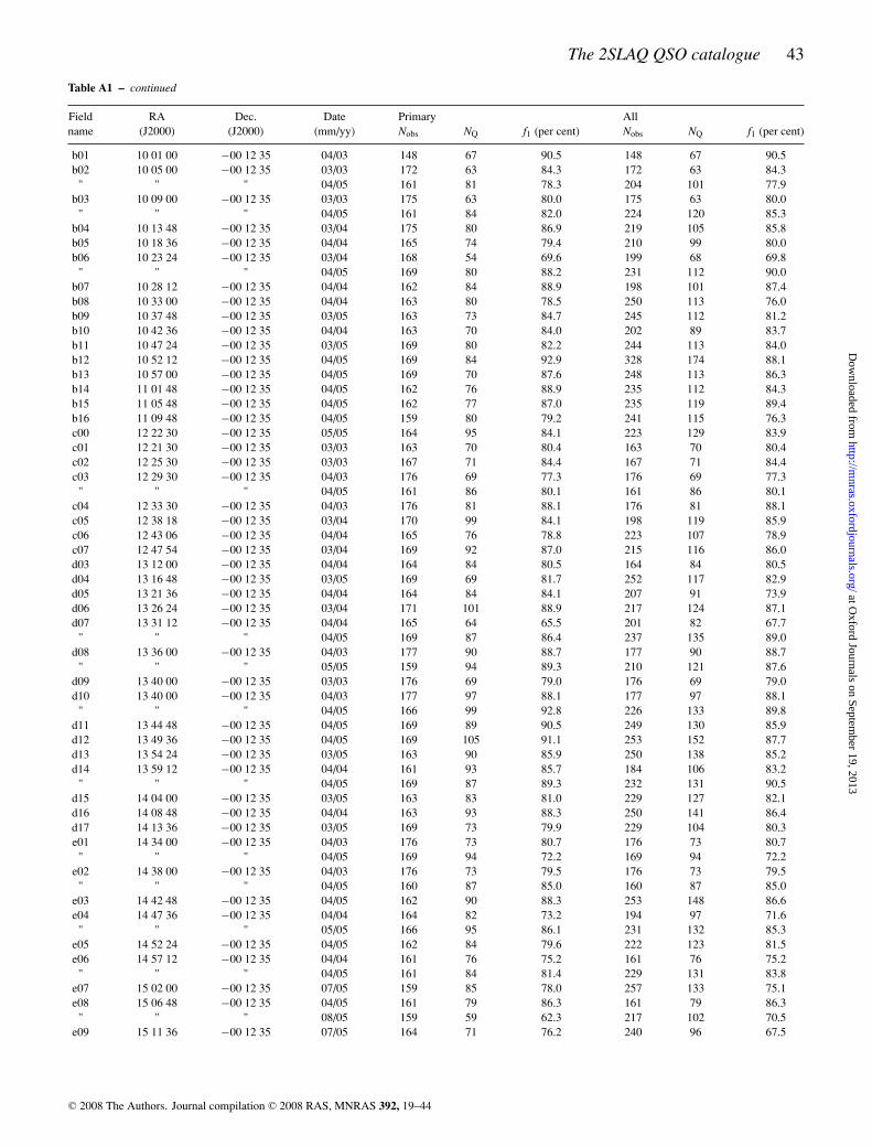
The 2SLAQ QSO catalogue 43
Table A1 – continued
Field RA Dec. Date Primary Allname (J2000) (J2000) (mm/yy) Nobs NQ f1 (per cent) Nobs NQ f1 (per cent)
b01 10 01 00 −00 12 35 04/03 148 67 90.5 148 67 90.5b02 10 05 00 −00 12 35 03/03 172 63 84.3 172 63 84.3
" " " 04/05 161 81 78.3 204 101 77.9b03 10 09 00 −00 12 35 03/03 175 63 80.0 175 63 80.0
" " " 04/05 161 84 82.0 224 120 85.3b04 10 13 48 −00 12 35 03/04 175 80 86.9 219 105 85.8b05 10 18 36 −00 12 35 04/04 165 74 79.4 210 99 80.0b06 10 23 24 −00 12 35 03/04 168 54 69.6 199 68 69.8
" " " 04/05 169 80 88.2 231 112 90.0b07 10 28 12 −00 12 35 04/04 162 84 88.9 198 101 87.4b08 10 33 00 −00 12 35 04/04 163 80 78.5 250 113 76.0b09 10 37 48 −00 12 35 03/05 163 73 84.7 245 112 81.2b10 10 42 36 −00 12 35 04/04 163 70 84.0 202 89 83.7b11 10 47 24 −00 12 35 03/05 169 80 82.2 244 113 84.0b12 10 52 12 −00 12 35 04/05 169 84 92.9 328 174 88.1b13 10 57 00 −00 12 35 04/05 169 70 87.6 248 113 86.3b14 11 01 48 −00 12 35 04/05 162 76 88.9 235 112 84.3b15 11 05 48 −00 12 35 04/05 162 77 87.0 235 119 89.4b16 11 09 48 −00 12 35 04/05 159 80 79.2 241 115 76.3c00 12 22 30 −00 12 35 05/05 164 95 84.1 223 129 83.9c01 12 21 30 −00 12 35 03/03 163 70 80.4 163 70 80.4c02 12 25 30 −00 12 35 03/03 167 71 84.4 167 71 84.4c03 12 29 30 −00 12 35 04/03 176 69 77.3 176 69 77.3
" " " 04/05 161 86 80.1 161 86 80.1c04 12 33 30 −00 12 35 04/03 176 81 88.1 176 81 88.1c05 12 38 18 −00 12 35 03/04 170 99 84.1 198 119 85.9c06 12 43 06 −00 12 35 04/04 165 76 78.8 223 107 78.9c07 12 47 54 −00 12 35 03/04 169 92 87.0 215 116 86.0d03 13 12 00 −00 12 35 04/04 164 84 80.5 164 84 80.5d04 13 16 48 −00 12 35 03/05 169 69 81.7 252 117 82.9d05 13 21 36 −00 12 35 04/04 164 84 84.1 207 91 73.9d06 13 26 24 −00 12 35 03/04 171 101 88.9 217 124 87.1d07 13 31 12 −00 12 35 04/04 165 64 65.5 201 82 67.7
" " " 04/05 169 87 86.4 237 135 89.0d08 13 36 00 −00 12 35 04/03 177 90 88.7 177 90 88.7
" " " 05/05 159 94 89.3 210 121 87.6d09 13 40 00 −00 12 35 03/03 176 69 79.0 176 69 79.0d10 13 40 00 −00 12 35 04/03 177 97 88.1 177 97 88.1
" " " 04/05 166 99 92.8 226 133 89.8d11 13 44 48 −00 12 35 04/05 169 89 90.5 249 130 85.9d12 13 49 36 −00 12 35 04/05 169 105 91.1 253 152 87.7d13 13 54 24 −00 12 35 03/05 163 90 85.9 250 138 85.2d14 13 59 12 −00 12 35 04/04 161 93 85.7 184 106 83.2
" " " 04/05 169 87 89.3 232 131 90.5d15 14 04 00 −00 12 35 03/05 163 83 81.0 229 127 82.1d16 14 08 48 −00 12 35 04/04 163 93 88.3 250 141 86.4d17 14 13 36 −00 12 35 03/05 169 73 79.9 229 104 80.3e01 14 34 00 −00 12 35 04/03 176 73 80.7 176 73 80.7
" " " 04/05 169 94 72.2 169 94 72.2e02 14 38 00 −00 12 35 04/03 176 73 79.5 176 73 79.5
" " " 04/05 160 87 85.0 160 87 85.0e03 14 42 48 −00 12 35 04/05 162 90 88.3 253 148 86.6e04 14 47 36 −00 12 35 04/04 164 82 73.2 194 97 71.6
" " " 05/05 166 95 86.1 231 132 85.3e05 14 52 24 −00 12 35 04/05 162 84 79.6 222 123 81.5e06 14 57 12 −00 12 35 04/04 161 76 75.2 161 76 75.2
" " " 04/05 161 84 81.4 229 131 83.8e07 15 02 00 −00 12 35 07/05 159 85 78.0 257 133 75.1e08 15 06 48 −00 12 35 04/05 161 79 86.3 161 79 86.3
" " " 08/05 159 59 62.3 217 102 70.5e09 15 11 36 −00 12 35 07/05 164 71 76.2 240 96 67.5
C© 2008 The Authors. Journal compilation C© 2008 RAS, MNRAS 392, 19–44
at Oxford Journals on Septem
ber 19, 2013http://m
nras.oxfordjournals.org/D
ownloaded from
44 S. M. Croom et al.
Table A1 – continued
Field RA Dec. Date Primary Allname (J2000) (J2000) (mm/yy) Nobs NQ f1 (per cent) Nobs NQ f1 (per cent)
e10 15 16 24 −00 12 35 08/05 164 65 64.0 198 87 68.7s06 21 21 36 −00 15 00 09/03 172 60 80.8 172 60 80.8s07 21 26 24 −00 15 00 10/04 168 56 67.9 243 88 66.7" " " 07/05 159 61 69.2 207 93 73.9
s08 21 31 12 −00 15 00 10/04 171 54 80.1 222 67 74.3s09 21 36 00 −00 15 00 10/04 168 32 39.3 168 32 39.3" " " 08/05 159 47 72.3 196 63 73.5
s10 21 40 48 −00 15 00 07/05 165 60 72.1 224 84 71.4s11 21 45 36 −00 15 00 07/05 164 61 72.0 224 82 68.3s12 21 50 24 −00 15 00 08/03 176 45 71.0 176 45 71.0s25 22 52 48 −00 15 00 08/03 176 87 85.2 176 87 85.2s26 22 57 36 −00 15 00 10/04 150 59 61.3 150 59 61.3" " " 08/05 164 81 68.3 164 81 68.3
s27 23 02 24 −00 15 00 09/03 175 82 80.0 175 82 80.0s28 23 07 12 −00 15 00 10/04 150 74 74.7 176 93 75.6s29 23 12 00 −00 15 00 10/04 156 81 88.5 215 112 89.8s30 23 16 48 −00 15 00 10/04 150 84 90.0 212 113 88.2s31 23 21 36 −00 15 00 07/05 159 89 84.3 208 113 83.7s32 23 26 24 −00 15 00 08/05 159 94 86.2 198 117 87.4s47 00 38 24 −00 15 00 08/05 164 86 80.5 234 131 79.5s48 00 43 12 −00 15 00 10/04 171 86 83.0 271 145 82.7s49 00 48 00 −00 15 00 10/04 168 69 60.7 168 69 60.7s50 00 52 48 −00 15 00 08/03 174 76 84.5 174 76 84.5s51 00 57 36 −00 15 00 10/04 167 79 85.0 228 108 85.1s52 01 02 24 −00 15 00 09/03 172 72 79.7 172 72 79.7s67 02 14 24 −00 15 00 10/04 156 72 82.7 241 100 74.3s68 02 19 12 −00 15 00 10/04 150 51 53.3 150 51 53.3s69 02 24 00 −00 15 00 09/03 173 52 64.7 173 52 64.7s70 02 28 48 −00 15 00 10/04 150 63 83.3 213 90 77.5
SUPPORTING INFORMATION
Additional Supporting Information may be found in the online ver-sion of this article.
Table 12. The 2SLAQ colour completeness array. The completenessis given as a function of redshift, z, and g-band magnitude. We alsolist the host-galaxy contribution as a magnitude difference, �hostin both the g and i bands.
Table S1. The 2SLAQ QSO catalogue. The entries in this catalogueare described in Table 5.
Table S2. The 2SLAQ QSO repeated objects catalogue. The entriesin this catalogue are described in Table 5.
Please note: Wiley-Blackwell are not responsible for the content orfunctionality of any supporting materials supplied by the authors.Any queries (other than missing material) should be directed to thecorresponding author for the article.
This paper has been typeset from a TEX/LATEX file prepared by the author.
C© 2008 The Authors. Journal compilation C© 2008 RAS, MNRAS 392, 19–44
at Oxford Journals on Septem
ber 19, 2013http://m
nras.oxfordjournals.org/D
ownloaded from