Open Research OnlineThe Open University’s repository of research publicationsand other research outputs

Latin Americans show wide-spread Converso ancestryand imprint of local Native ancestry on physicalappearanceJournal ItemHow to cite:

Chacón-Duque, Juan-Camilo; Adhikari, Kaustubh; Fuentes-Guajardo, Macarena; Mendoza-Revilla, Javier; Acuña-Alonzo, Victor; Barquera, Rodrigo; Quinto-Sánchez, Mirsha; Gómez-Valdés, Jorge; Everardo Martínez, Paola;Villamil-Ramírez, Hugo; Hünemeier, Tábita; Ramallo, Virginia; Silva de Cerqueira, Caio C.; Hurtado, Malena; Villegas,Valeria; Granja, Vanessa; Villena, Mercedes; Vásquez, René; Llop, Elena; Sandoval, José R.; Salazar-Granara, AlbertoA.; Parolin, Maria-Laura; Sandoval, Karla; Peñaloza-Espinosa, Rosenda I.; Rangel-Villalobos, Hector; Winkler, CherylA.; Klitz, William; Bravi, Claudio; Molina, Julio; Corach, Daniel; Barrantes, Ramiro; Gomes, Verónica; Resende,Carlos; Gusmão, Leonor; Amorim, Antonio; Xue, Yali; Dugoujon, Jean-Michel; Moral, Pedro; González-José, Rolando;Schuler-Faccini, Lavinia; Salzano, Francisco M.; Bortolini, Maria-Cátira; Canizales-Quinteros, Samuel; Poletti,Giovanni; Gallo, Carla; Bedoya, Gabriel; Rothhammer, Francisco; Balding, David; Hellenthal, Garrett and Ruiz-Linares,Andrés (2018). Latin Americans show wide-spread Converso ancestry and imprint of local Native ancestry on physicalappearance. Nature Communications, 9, article no. 5388.

For guidance on citations see FAQs.

c© 2018 The Author(s)

https://creativecommons.org/licenses/by/4.0/

Version: Supplementary Material

Link(s) to article on publisher’s website:http://dx.doi.org/doi:10.1038/s41467-018-07748-z

Copyright and Moral Rights for the articles on this site are retained by the individual authors and/or other copyrightowners. For more information on Open Research Online’s data policy on reuse of materials please consult the policiespage.

oro.open.ac.uk

Supplementary Information

Latin Americans show wide-spread Converso ancestry and

imprint of local Native ancestry on physical appearance

Chacón-Duque et al.

2

TABLE OF CONTENTS

SUPPLEMENTARY FIGURES 5

Supplementary Figure 1. Birthplace of the CANDELA individuals included in this study 5

Supplementary Figure 2. Approximate geographic location of the 117 reference

population samples used in this study 6

Supplementary Figure 3. Tree relating the 56 surrogate clusters defined by

fineSTRUCTURE and retained for ancestry inference 7

Supplementary Figure 4. Percentage of Native American ancestry sub-components for

377 Brazilians with >5% Native American ancestry, as inferred by SOURCEFIND 8

Supplementary Figure 5. Geographic distribution of Sub-Saharan African ancestry sub-

components in CANDELA individuals, as inferred by SOURCEFIND 9

Supplementary Figure 6. Differences in Sub-Saharan African sub-continental ancestry

between former Portuguese and Spanish colonies 10

Supplementary Figure 7. Geographic distribution of East Asian ancestry sub-components

in CANDELA individuals, as inferred by SOURCEFIND 11

Supplementary Figure 8. Unsupervised ADMIXTURE analysis from K=2 to K=10 12

Supplementary Figure 9. Principal Components Analysis 14

Supplementary Figure 10. Differences in allele frequencies between Mapuche and

Central Andean populations 19

Supplementary Figure 11. Average -log (p-values) for the differences in allele frequencies

between Mapuche and Central Andean populations across sets of six randomly selected

SNPs 20

Supplementary Figure 12. Global overview of the analysis strategy 21

Supplementary Figure 13. Overview of the analysis strategy for the definition of

homogeneous clusters of reference population individuals 22

Supplementary Figure 14. Example CANDELA individual for which GLOBETROTTER

infers admixture involving three sources at about the same time 23

SUPPLEMENTARY TABLES 24

Supplementary Table 1. 117 Reference population samples 24

Supplementary Table 2. Description of the decisions made on the clusters based on the

129 clusters generated by fineSTRUCTURE 28

Supplementary Table 3. Individuals from the 117 reference population samples included

in the 56 clusters defined by fineSTRUCTURE 35

Supplementary Table 4. Regression of Native American ancestry proportion on inferred

admixture date 37

3

Supplementary Table 5. Allele frequencies in the Central Andes and the Mapuche at

index SNPs associated with facial features in the CANDELA sample 38

Supplementary Table 6. Number of SNPs per GWAS hit matching the criteria to define

the sets of six randomly selected SNPs 39

Supplementary Table 7. Proportion of Self-copying in Native American surrogate

clusters 40

Supplementary Table 8. Proportion of inferred admixture events according to

GLOBETROTTER conclusion by different source groups 41

SUPPLEMENTARY NOTES 42

Supplementary Note 1. ADMIXTURE and Principal Components Analysis (PCA) 42

Supplementary Figure 15. Supervised ADMIXTURE analyses in the CANDELA 42

Supplementary Figure 16. Comparison of continental ancestry estimates for the

CANDELA sample obtained with SOURCEFIND and ADMIXTURE 43

Supplementary Note 2. Assessing the performance of NNLS, SOURCEFIND and

GLOBETROTTER through simulations 46

Simulations to assess the accuracy of sub-continental ancestry estimates 47

Supplementary Figure 17. Pyramid charts showing the distribution of simulated ancestry

proportions from each surrogate cluster across the 100 simulated individuals for scenario

(i) 48

Supplementary Figure 18. Pyramid charts showing the distribution of simulated ancestry

proportions from each surrogate cluster across the 100 simulated individuals for scenario

(ii) 50

Supplementary Figure 19. Pyramid charts showing the distribution of simulated ancestry

proportions from each surrogate cluster across the 100 simulated individuals for scenario

(iii) 51

Supplementary Figure 20. Pyramid charts showing the distribution of simulated ancestry

proportions from each surrogate cluster across the 100 simulated individuals for scenario

(iv) 52

Simulations to assess the accuracy of per individual estimation of time since admixture and

the effect of time since admixture on ancestry estimation 53

Supplementary Figure 21. GLOBETROTTER’s inferred dates (y-axis) across individuals,

for simulations mixing CentralSouthSpain and Quechua2 at the given proportions

(legend) and times (x-axis) 54

Supplementary Figure 22. SOURCEFIND's inferred proportion of ancestry related to

Iberian (IBR) and Native American (NAM) sources (y-axis) across individuals (circles),

for simulations mixing CentralSouthSpain and Quechua2 at the given proportions (x-axis)

and times (legend) 54

Supplementary Figure 23. Mean ancestry percentages in the simulated individuals

estimated by SOURCEFIND grouped by the number of generations since admixture 55

4

Supplementary Figure 24. GLOBETROTTER’s inferred dates (y-axis) across individuals,

for simulations with two sequential admixture events, at the given proportions (legend)

and times (x-axis). 56

Supplementary Figure 25. SOURCEFIND's inferred proportion of ancestry related to

Iberian (IBR) and Native American (NAM) sources (y-axis) across individuals (circles),

for simulations with two sequential admixture events, at the given proportions (x-axis)

and times (legend). 57

Supplementary Figure 26. Mean ancestry percentages in the simulated individuals for two

sequential admixture events estimated by SOURCEFIND, grouped by the number of

generations since admixture. 58

Assessing the reliability of East/South Mediterranean ancestry estimation 58

Supplementary Note 3. Average continental and sub-continental ancestry from

SOURCEFIND and ADMIXTURE 59

Supplementary Table 9. Average continental ancestry percentages estimated from

unsupervised ADMIXTURE at k=4, for each country and the overall CANDELA sample

59

Supplementary Table 10. Average continental ancestry percentages (corresponding to the

five major bio-geographical regions) obtained from SOURCEFIND, for each country and

the overall CANDELA sample 59

Supplementary Table 11. Average sub-continental ancestry percentages (for the 35

groups) obtained from SOURCEFIND, for each country and the overall CANDELA

sample 60

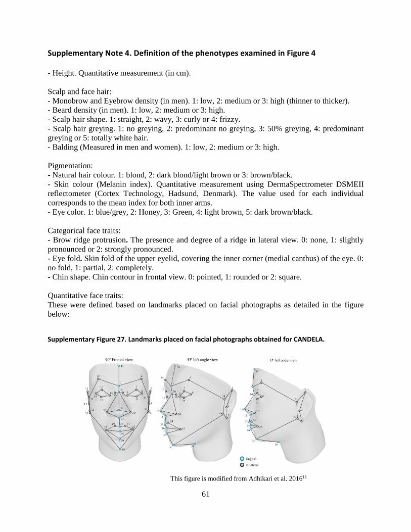
Supplementary Note 4. Definition of the phenotypes examined in Figure 4 61

Supplementary Figure 27. Landmarks placed on facial photographs obtained for

CANDELA. 61

Supplementary Figure 28. Ear traits characterized in the CANDELA dataset. 62

Supplementary Note 5. Correlation of regression p-values from different approaches to

the Central Andes - Mapuche ancestry contrast 63

Supplementary Table 12. Spearman’s rank correlations 63

Supplementary Note 6. Robustness of SOURCEFIND ancestry inference to the exclusion

CANDELA individuals used as reference samples 64

Supplementary Figure 29. Individual pie-maps showing SOURCEFIND analyses when

not including any CANDELA reference samples as surrogates or donors. 64

References 65

5

SUPPLEMENTARY FIGURES

Supplementary Figure 1. Birthplace of the CANDELA individuals included in this study

Circles are centred on birthplace with size proportional to the number of individuals born at that

location (scale provided on the left). A total of 6,589 individuals across five countries are shown.

6

Supplementary Figure 2. Approximate geographic location of the 117 reference population samples used in this study

Populations have been color-coded as: blue (38 Native American), red (42 European), yellow (15 East/South Mediterranean), green

(15 Sub-Saharan African) and purple (7 East Asians). Numbers inside the dots correspond to those used in Supplementary Table 1 with

additional information on these samples.

7

Supplementary Figure 3. Tree relating the 56 surrogate clusters defined by

fineSTRUCTURE and retained for ancestry inference

Brackets on the right indicate the 35 groups of clusters displayed in Figure 1.

8

Supplementary Figure 4. Percentage of Native American ancestry sub-components for

377 Brazilians with >5% Native American ancestry, as inferred by SOURCEFIND

The figure was made with ggplot2. The centre line corresponds to the median, the bounds of box

represent the first (𝑄1) and the third (𝑄3) quartiles, and the whiskers approximate to 𝑄1 -

1.5*Inter-Quartile Range and 𝑄3 + 1.5*Inter-Quartile Range. Outlying points are plotted

individually.

9

Supplementary Figure 5. Geographic distribution of Sub-Saharan African ancestry sub-

components in CANDELA individuals, as inferred by SOURCEFIND

This pie map follows the same convention of Figure 2. Each pie represents an individual, with pie

location corresponding to birthplace. Since many individuals share birthplace, jittering has been

performed based on pie size and how crowded an area is. Pie size is proportional to total ancestry

from all sources depicted in that specific figure, and only individuals with >5% of such total

ancestry are shown. Coloring of pies represents the proportion of each sub-continental component

estimated for each individual (color-coded as in Fig. 1).

10

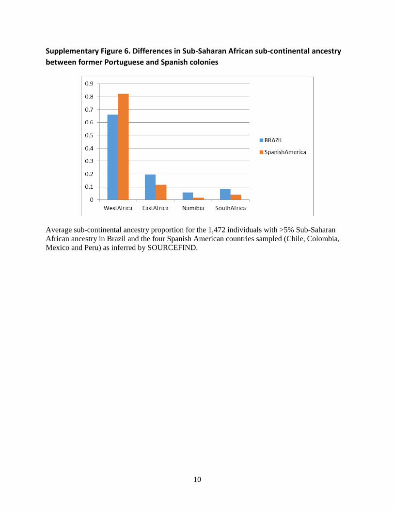
Supplementary Figure 6. Differences in Sub-Saharan African sub-continental ancestry

between former Portuguese and Spanish colonies

Average sub-continental ancestry proportion for the 1,472 individuals with >5% Sub-Saharan

African ancestry in Brazil and the four Spanish American countries sampled (Chile, Colombia,

Mexico and Peru) as inferred by SOURCEFIND.

11

Supplementary Figure 7. Geographic distribution of East Asian ancestry sub-

components in CANDELA individuals, as inferred by SOURCEFIND

This pie map follows the same convention of Figure 2. Each pie represents an individual, with pie

location corresponding to birthplace. Since many individuals share birthplace, jittering has been

performed based on pie size and how crowded an area is. Pie size is proportional to total ancestry

from all sources depicted in that specific figure, and only individuals with >5% of such total

ancestry are shown. Coloring of pies represents the proportion of each sub-continental component

estimated for each individual (color-coded as in Fig. 1).

12

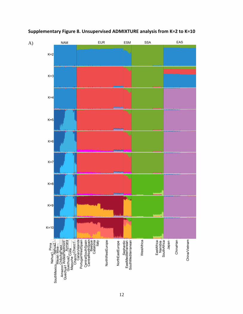
Supplementary Figure 8. Unsupervised ADMIXTURE analysis from K=2 to K=10

A)

13

B)

(A) 1,444 reference samples included in the 35 surrogate groups and (B) the 6,561 CANDELA

individuals included in the SOURCEFIND analyses. In (B) CANDELA individuals are shown on

the left, grouped by country of birthplace. On the right, the figure (A) is replicated but the

reference are grouped by major geographic region (NAM = Native American, EUR = European,

ESM = East/South Mediterranean, SSA = Sub-Saharan African, EAS = East Asian), sub-grouped

according to the 35 surrogate groups defined by fineSTRUCTURE (Supplementary Fig. 3).

14

Supplementary Figure 9. Principal Components Analysis

A)

B)

15

C)

D)

16

E)

F)

17

G)

H)

18

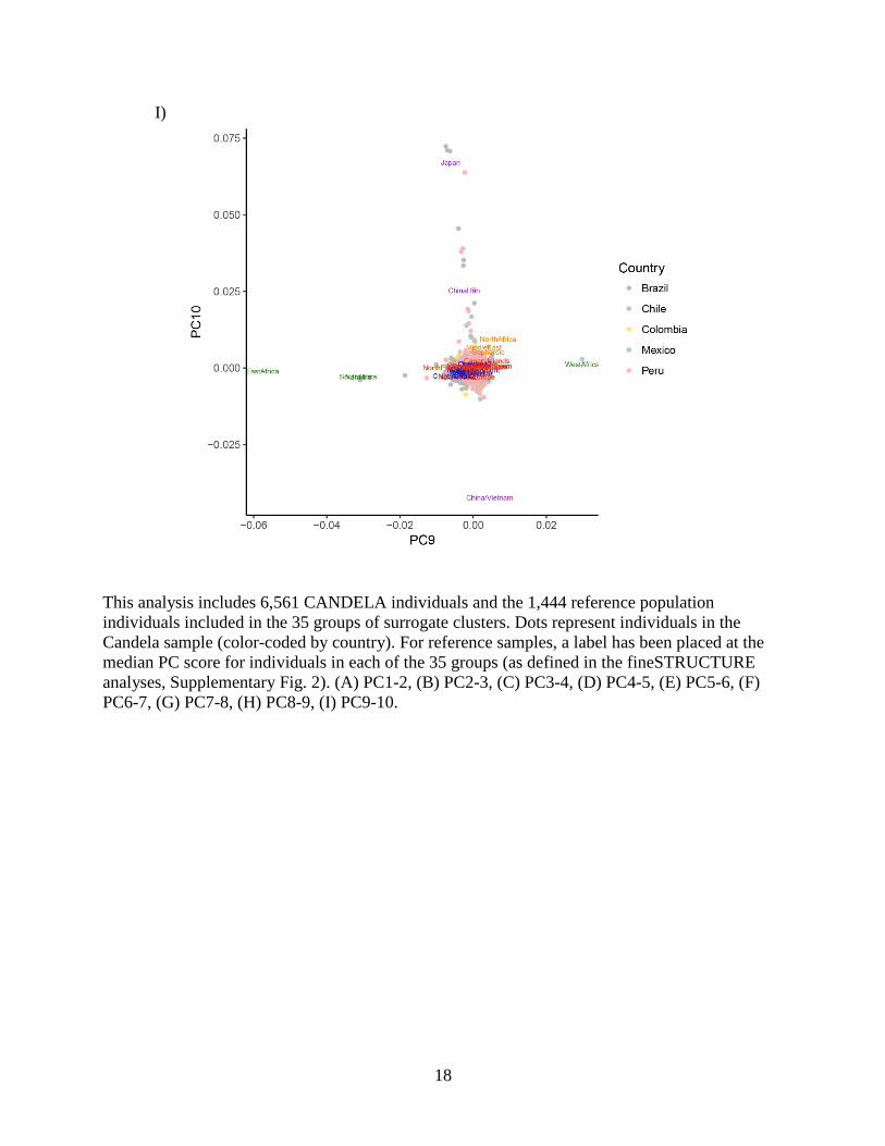
I)

This analysis includes 6,561 CANDELA individuals and the 1,444 reference population

individuals included in the 35 groups of surrogate clusters. Dots represent individuals in the

Candela sample (color-coded by country). For reference samples, a label has been placed at the

median PC score for individuals in each of the 35 groups (as defined in the fineSTRUCTURE

analyses, Supplementary Fig. 2). (A) PC1-2, (B) PC2-3, (C) PC3-4, (D) PC4-5, (E) PC5-6, (F)

PC6-7, (G) PC7-8, (H) PC8-9, (I) PC9-10.

19

Supplementary Figure 10. Differences in allele frequencies between Mapuche and

Central Andean populations

A two-sample t-test –log10(p-values) across all SNPs, when testing whether each SNP’s allele

frequency for inferred Mapuche segments is the same as that for inferred Central Andean

segments. Dashed blue lines denote the six GWAS hit SNPs associated with facial features, and

red lines the mean across these.

20

Supplementary Figure 11. Average -log (p-values) for the differences in allele

frequencies between Mapuche and Central Andean populations across sets of six

randomly selected SNPs

A)

B)

10,000 sets of six randomly selected SNPs that match the number of inferred Mapuche and

Central Andean segments at the six GWAS hit SNPs, plus match the minor allele frequency of

either the inferred (A) Central Andean or (B) Mapuche segments at the six GWAS hit SNPs.

Dashed red lines give the average -log10(p-value) across the six GWAS hit SNPs, and p-value

gives the proportion of random samples with average -log10(p-values) greater than the dashed

red line.

21

Supplementary Figure 12. Global overview of the analysis strategy

Yellow trapezoids represent the data used and/or generated, blue rectangles the implemented

analyses/approaches and Green diamonds the results obtained from the different

analyses/approaches.

22

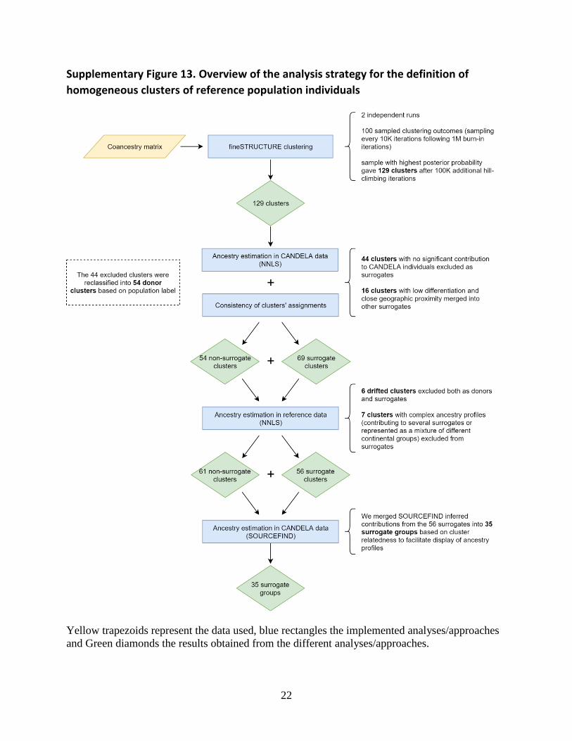
Supplementary Figure 13. Overview of the analysis strategy for the definition of

homogeneous clusters of reference population individuals

Yellow trapezoids represent the data used, blue rectangles the implemented analyses/approaches

and Green diamonds the results obtained from the different analyses/approaches.

23

Supplementary Figure 14. Example CANDELA individual for which GLOBETROTTER

infers admixture involving three sources at about the same time

A) B)

C)

Dots are the inferred relative probabilities that a pair of DNA segments in this individual are

inherited from: (A) Native American (NAM) and European (EUR) sources, (B) NAM and Sub-

Saharan African (SSA) sources, (C) EUR and SSA sources, as a function of the genetic distance

between the DNA segments. The fitted exponential curves result in an estimated admixture date

of 11 generations ago.

24

SUPPLEMENTARY TABLES

Supplementary Table 1. 117 Reference population samples

n Sample label Group* N (Pre-QC)

N (Post-QC)

Country of origin (.sample)

Data source (reference)

1 Pima NAM 2 2 Mexico.1 1

2 Nahua NAM 25 25 Mexico.2 This study

3 Mixe NAM 2 2 Mexico.3 1

4 Mixe.B NAM 16 16 Mexico.4 This study

5 Mixtec NAM 2 2 Mexico.5 1

6 Mixtec.B NAM 10 10 Mexico.6 This study

7 Zapotec NAM 2 2 Mexico.7 1

8 Zapotec.B NAM 12 12 Mexico.8 This study

9 Mayan NAM 2 2 Mexico.9 1

10 Kaqchikel NAM 8 8 Guatemala This study

11 Cabecar NAM 5 5 Costa.Rica.1 This study

12 Guaymi NAM 4 4 Costa.Rica.2 This study

13 Embera NAM 21 21 Colombia.1 This study

14 Waunana NAM 5 5 Colombia.2 This study

15 Wayuu NAM 3 3 Colombia.3 This study

16 Kogi NAM 6 6 Colombia.4 This study

17 Zenu NAM 7 7 Colombia.5 This study

18 Piapoco NAM 2 2 Colombia.6 1

19 Ticuna NAM 4 4 Colombia.7 This study

20 Inga NAM 3 3 Colombia.8 This study

21 Karitiana NAM 3 3 Brazil.1 1

22 Surui NAM 2 2 Brazil.2 1

23 Xavante NAM 4 4 Brazil.3 This study

24 Andoa NAM 20 20 Peru.1 This study

25 Aymara.A NAM 13 13 Bolivia.1 This study

26 Aymara.B NAM 4 4 Chile.1 This study

27 Quechua NAM 3 3 Peru.2 1

28 Quechua.B NAM 14 14 Bolivia.2 This study

29 Uros NAM 8 8 Peru.3 This study

30 Colla NAM 25 23 Argentina.1 2

31 Wichi NAM 25 19 Argentina.3 2

32 Wichi.B NAM 4 4 Argentina.4 This study

33 Toba NAM 4 4 Argentina.5 This study

34 Ache NAM 5 5 Paraguay This study

35 Guarani NAM 5 5 Argentina.6 This study

25

36 Chane NAM 2 2 Argentina.7 This study

37 Mapuche NAM 9 9 Argentina.2 This study

38 Huilliche NAM 10 10 Chile.2 This study

39 PRT.A EUR 18 18 Portugal.1 This study

40 PRT.B EUR 31 31 Portugal.2 This study

41 IBS-Galicia EUR 12 8 Spain.1 3

42 SP-CAN EUR 14 14 Spain.2 This study

43 IBS-Canarias EUR 3 2 Spain.3 3

44 SP-AND EUR 15 15 Spain.4 This study

45 IBS-Andalucia EUR 4 4 Spain.5 3

46 IBS-Extremadura EUR 12 8 Spain.6 3

47 IBS EUR 7 7 Spain.7 3

48 SP-CSP EUR 15 15 Spain.8 This study

49 IBS-Cast.Leon EUR 18 12 Spain.9 3

50 IBS-Cast.Mancha EUR 9 6 Spain.10 3

51 IBS-Murcia EUR 12 8 Spain.11 3

52 IBS-Valencia EUR 21 14 Spain.12 3

53 IBS-Aragon EUR 6 6 Spain.13 3

54 SP-CTL EUR 7 7 Spain.14 This study

55 IBS-Cataluna EUR 15 10 Spain.15 3

56 IBS-Baleares EUR 12 8 Spain.16 3

57 IBS-Cantabria EUR 9 6 Spain.17 3

58 SP-BAS EUR 14 14 Spain.18 This study

59 IBS-Pais.Vasco EUR 12 8 Spain.19 3

60 Basque EUR 2 2 France.1 1

61 French EUR 3 3 France.2 1

62 Bergamo EUR 2 2 Italy.1 1

63 Sardinian EUR 3 3 Italy.2 1

64 TSI EUR 107 106 Italy.3 3

65 Tuscan EUR 2 2 Italy.4 1

66 CEU EUR 99 91 NW.Europe 3

67 GBR-Kent EUR 38 31 UK.1 3

68 GBR-Cornwall EUR 32 29 UK.2 3

69 GBR-Corn-Devon EUR 1 1 UK.3 3

70 GBR-Scotland EUR 4 3 UK.4 3

71 Orcadian EUR 2 2 UK.5 1

72 GBR-Orkney EUR 26 21 UK.6 3

73 Bulgarian EUR 2 2 Bulgaria 1

74 Hungarian EUR 2 2 Hungary 1

75 Greek EUR 2 2 Greece.1 1

76 Crete EUR 2 2 Greece.2 1

26

77 Georgian EUR 2 2 Georgia 1

78 FIN EUR 99 99 Finland 3

79 Estonian EUR 2 2 Estonia 1

80 Russian EUR 2 2 Russia 1

81 MRC ESM 14 11 Morocco.1 This study

82 Moroccan_Jew# ESM 7 7 Morocco.2 This study

83 TUN ESM 14 14 Tunisia.1 This study

84 Tunisian_Jew# ESM 6 6 Tunisia.2 This study

85 LIB ESM 15 14 Libya.1 This study

86 Libyan_Jew# ESM 7 7 Libya.2 This study

87 JRD ESM 15 15 Jordan.1 This study

88 Sephardi_Jew# ESM 7 7 Turkey.1 This study

89 Turkish ESM 2 2 Turkey.2 1

90 BedouinB ESM 2 2 Israel.1 1

91 Druze ESM 2 2 Israel.2 1

92 Iraqi_Jew ESM 2 2 Iraq 1

93 Jordanian ESM 3 3 Jordan.2 1

94 Palestinian ESM 3 3 Palestine 1

95 Yemenite_Jew ESM 2 2 Yemen 1

96 YRI SSA 108 101 Nigeria.1 3

97 ESN SSA 99 95 Nigeria.2 3

98 GWD SSA 113 111 Gambia 3

99 MSL SSA 85 69 Sierra.Leone 3

100 LWK SSA 99 73 Kenya 3

101 Anuak SSA 21 3 Ethiopia 4

102 South_Sudanese SSA 21 8 South.Sudan 4

103 GuiGhanaKgal SSA 15 14 Botswana 5

104 Juhoansi SSA 18 15 Namibia.1 5

105 Karretjie SSA 20 3 South.Africa.1 5

106 Khomani SSA 39 4 South.Africa.2 5

107 Khwe SSA 17 14 Namibia.2 5

108 SEBantu SSA 20 19 South.Africa.3 5

109 SWBantu SSA 12 9 Namibia.3 5

110 Xun SSA 19 19 Angola 5

111 KHV EAS 99 95 Vietnam 3

112 CDX EAS 93 82 China.1 3

113 CHS-Hu_Nan EAS 102 66 China.2 3

114 CHS-Fu_Jian EAS 48 31 China.3 3

115 CHB EAS 103 101 China.4 3

116 Korean EAS 2 2 Korea 1

117 JPT EAS 104 104 Japan 3

27

Total 2359 2058

Note: Genotypes at SNPs shared between published datasets were reported to have been obtained

by full genome sequencing (1) or genotyping on the following platforms: (2) Illumina

OmniExpress, (3) Illumina Omni2.5M, (4) Illumina Omni1M, (5) Illumina Omni2.5M.

References: (1) Mallick S et al 20161, (2) Eichstaedt CA et al. 20142, (3) 1000 genomes project3,

(4) Pagani L et al. 20124 and (5) Schlebusch CM et al. 20125.

* NAM: Native American, EUR: European, ESM: East/South Mediterranean, SSA: Sub-Saharan

African, EAS: East Asian.

# Samples obtained from The National Laboratory for the Genetics of Israeli Populations

(http://yoran.tau.ac.il/nlgip/).

28

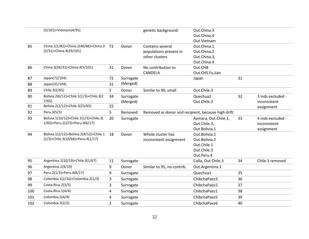
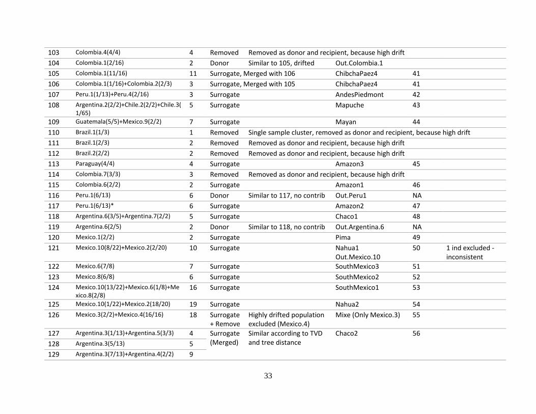
Supplementary Table 2. Description of the decisions made on the clusters based on the 129 clusters generated by

fineSTRUCTURE

fS Clust

Contains N Decision Explanation of decision Donor/Surrogate Surrog Additional notes

1 South.Sudan(1/8) 1 Donor Single sample cluster Out.SouthSudan

2 Ethiopia(3/3)+South.Sudan(7/8) 10 Surrogate EastAfrica1 1

3 Kenya(35/73) 35 Surrogate (Merged)

Similar according to TVD and tree distance

EastAfrica2 2 No clear assignment 4 Kenya(38/73) 38

5 Namibia.3(1/9) 1 Donor Single sample cluster Out.Namibia.3

6 Namibia.3(1/9)* 1 Donor Single sample cluster Out.Namibia.3

7 Namibia.3(6/9) 6 Surrogate Namibia 3

8 Namibia.2(1/14)+Namibia.3(1/9) 2 Donor Similar to 7, no contribution

Out.Namibia.2 Out.Namibia.3

9 South.Africa.3(1/19) 1 Donor Single sample cluster Out.South.Africa.3

10 Namibia.2(1/14) 1 Donor Single sample cluster Out.Namibia.2

11 Namibia.2(6/14) 6 Donor No contribution Out.Namibia.2

12 Namibia.2(5/14) 5 Donor No contribution Out.Namibia.2

13 South.Africa.3(10/19) 10 Surrogate (Merged)

Similar according to TVD and tree distance

SouthAfrica 4

14 South.Africa.3(8/19) 8

15 Gambia(3/111)+Sierra.Leone(1/69) 4 Donor Similar to 18, small Out.Gambia Out.SierraLeone

16 Gambia(10/111) 10 Donor Similar to 18, small Out.Gambia

17 Gambia(18/111) 18 Donor Similar to 18, small Out.Gambia

18 Gambia(29/111) 29 Surrogate (Merged)

Similar according to TVD and tree distance

WestAfrica1 5

19 Gambia(22/111) 22

20 Gambia(29/111)* 29 Donor Similar to 18, small Out.Gambia

21 Sierra.Leone(68/69) 68 Surrogate WestAfrica2 6

22 Nigeria.1(31/101)+Nigeria.2(1/95) 32 Surrogate (Merged)

Similar according to TVD and tree distance

WestAfrica3 Out.Nigeria.1 Out.Nigeria.2

7 2 Nigeria.2 and 1 inconsistent ind excluded

23 Nigeria.1(69/101)+Nigeria.2(1/95) 70

29

24 Nigeria.1(1/101)+Nigeria.2(93/95) 94 Donor Similar to 23 Out.Nigeria.1 Out.Nigeria.2

25 Botswana(1/14) 1 Donor Single sample cluster Out.Botswana

26 Botswana(1/14)* 1 Donor Single sample cluster Out.Botswana

27 Botswana(1/14)** 1 Donor Single sample cluster Out.Botswana

28 Botswana(3/14) 3 Donor No contribution Out.Botswana

29 South.Africa.1(1/3) 1 Donor Single sample cluster Out.South.Africa.1

30 South.Africa.2(1/4) 1 Donor Single sample cluster Out.South.Africa.2

31 Botswana(3/14)* 3 Donor No contribution Out.Botswana

32 Botswana(5/14) 5 Donor No contribution Out.Botswana

33 South.Africa.1(2/3)+South.Africa.2 (3/4)

5 Donor No contribution Out.South.Africa.1 Out.South.Africa.2

34 Angola(1/19)+Namibia.1(1/15) 2 Donor No contribution Out.Angola Out.Namibia.1

35 Angola(8/19) 8 Donor No contribution Out.Angola

36 Angola(10/19)+Namibia.2(1/14) 11 Donor No contribution Out.Angola Out.Namibia.2

37 Namibia.1(14/15) 14 Donor No contribution Out.Namibia.1

38 Jordan.1(1/15) 1 Donor Single sample cluster Out.Jordan.1

39 Israel.1(2/2)+Jordan.1(2/15) 4 Donor Similar to 41 Out.Israel.1 Out.Jordan.1

40 Jordan.1(2/15) 2 Donor Small cluster, similar 41 Out.Jordan.1

41 Jordan.1(7/15)+Yemen(2/2) 9 Surrogate EastMediterranean1 8

42 Jordan.1(1/15)+Jordan.2(3/3)+Palestine(3/3)

7 Surrogate EastMediterranean2 9

43 Turkey.2(2/2) 2 Donor Complex genetic profile Out.Turkey.2

44 Georgia(2/2)+Greece.1(1/2)+Greece.2(2/2)

5 Donor Complex genetic profile Out.Georgia Out.Greece.1 Out.Greece.2

45 Iraq(2/2)+Israel.2(2/2)+Jordan.1(2/15) 6 Donor Complex genetic profile Out.Iraq, Out.Israel.2 Out.Jordan.1

46 Morocco.2(7/7) 7 Surrogate Sephardic3 10

30

47 Libya.2(1/7)+Turkey.1(7/7) 8 Surrogate Sephardic1 11

48 Tunisia.2(4/6) 4 Surrogate (Merged)

Similar according to TVD and tree distance

Sephardic2 12

49 Libya.2(6/7)+Tunisia.2(2/6) 8

50 Libya.1(1/14)+Tunisia.1(2/14) 3 Surrogate (Merged)

Similar according to TVD and tree distance

SouthMediterranean1 13

51 Libya.1(11/14)+Tunisia.1(3/14) 14

52 Libya.1(2/14)+Tunisia.1(9/14) 11

53 Morocco.1(3/11) 3 Surrogate (Merged)

Similar according to TVD and tree distance

SouthMediterranean2 14

54 Morocco.1(8/11) 8

55 Spain.4(2/15) 2 Donor Similar to 56, small Out.Spain.4

56 Spain.10(4/6)+Spain.11(5/8)+Spain.12(3/14)+Spain.14(1/7)+Spain.2(1/14)+Spain.4(13/15)+Spain.5(4/4)+Spain.6(4/8)+Spain.7(4/7)+Spain.9(5/12)

44 Surrogate CentralSouthSpain Out.Spain.5 Out.Spain.10

15 2 inds excluded - inconsistent assignment

57 Spain.10(2/6)+Spain.12(6/14)+Spain.13(5/6)+Spain.17(6/6)+Spain.8(3/15)

22 Surrogate CentralNorthSpain Out.Spain.8 Out.Spain.12 Out.Spain.17

16 4 inds excluded - inconsistent assignment

58 Spain.8(12/15) 12 Donor Drifted, no contribution Out.Spain.8

59 Italy.2(3/3) 3 Donor Complex genetic profile Out.Italy.2

60 Spain.1(2/8)+Spain.11(1/8)+Spain.12(5/14)+Spain.13(1/6)+Spain.14(6/7)+Spain.15(10/10)+Spain.16(7/8)+Spain.7(3/7)+Spain.9(1/12)

36 Surrogate Catalonia Out.Spain.1 Out.Spain.11 Out.Spain.12

17 3 inds relocated to 56, 4 inds excluded - inconsistent

61 Portugal.2(1/31)+Spain.11(2/8)+Spain.2(13/14)+Spain.3(2/2)+Spain.6(1/8)

19 Surrogate CanaryIslands 18 1 ind relocated to 62

62 Portugal.1(18/18)+Portugal.2(30/31)+Spain.1(6/8)+Spain.16(1/8)+Spain.6(3/8)+Spain.9(6/12)

64 Surrogate Portugal/WestSpain Out.Spain.1 Out.Spain.9 Out.Spain.6 Out.Spain.16

19 3 inds relocated to 56, 9 inds excluded - inconsistent assignment

63 France.1(1/2)+Spain.18(1/14)+Spain.19(8/8)

10 Surrogate (Merged)

Similar according to TVD and tree distance

Basque 20

64 France.1(1/2)+Spain.18(13/14) 14

31

65 Bulgaria(2/2)+Greece.1(1/2)+Italy.1(2/2)+Italy.5(15/15)

20 Surrogate Italy1 Out.Greece.1

21 1 Greece.1 ind removed

66 Italy.3(31/106) 31 Surrogate Italy2 22

67 Italy.3(75/106)+Italy.4(2/2) 77 Donor No contribution Out.Italy.3,Out.Italy.4

68 UK.2(28/29) 28 Donor Similar to 69, no contrib. Out.UK.2

69 France.2(1/3)+NW.Europe(74/91)+UK.1(31/31)+UK.2(1/29)+UK.3(1/1)+UK.4(3/3)

111 Surrogate NorthWestEurope2 Out.UK.4 Out.NW.Europe Out.France.2

23 10 inds excluded - inconsistent assignment

70 Germany(6/37)+Hungary(1/2)+NW.Europe(10/91)

17 Donor Similar to 69, small contribution to CANDELA

Out.Germany Out.Hungary Out.NW.Europe

71 UK.5(2/2)+UK.6(21/21) 23 Donor No contribution Out.UK.5, Out.UK.6

72 France.2(2/3)+Germany(31/37)+Hungary(1/2)+NW.Europe(7/91)

41 Surrogate NorthWestEurope1 Out.Hungary Out.France.2 Out.NW.Europe

24 Non-Germany indivudals removed

73 Russia(2/2) 2 Surrogate NorthEastEurope1 25

74 Estonia(2/2)+Finland(7/99) 9 Surrogate NorthEastEurope2 26

75 Finland(29/99) 29 Surrogate (Merged)

Similar according to TVD and tree distance

NorthEastEurope3 27

76 Finland(41/99) 41

77 Finland(22/99) 22

78 China.1(2/82) 2 Donor Similar to 79, small Out.China.1

79 China.1(72/82) 72 Surrogate China/Vietnam1 28

80 China.1(7/82) 7 Donor Similar to 79, small Out.China.1

81 Vietnam(91/95) 91 Surrogate China/Vietnam2 29

82 Japan(1/104)+Korea(1/2) 2 Donor Samples represented by different clusters

Out.Japan Out.Korea

83 China.3(1/31)+China.4(64/101)+Korea(1/2)

66 Surrogate ChinaHan Out.China.3 Out.Korea

30 2 non China.4 inds removed

84 China.2(26/66)+China.3(2/31)+China.4 35 Donor Similar to 84, complex Out.China.2

32

(3/101)+Vietnam(4/95) genetic background Out.China.3 Out.China.4 Out.Vietnam

85 China.1(1/82)+China.2(40/66)+China.3(2/31)+China.4(29/101)

72 Donor Contains several populations present in other clusters

Out.China.1 Out.China.2 Out.China.3, Out.China.4

86 China.3(26/31)+China.4(5/101) 31 Donor No contribution to CANDELA

Out.CHB Out.CHS.Fu.Jian

87 Japan(72/104) 72 Surrogate (Merged)

Japan 31

88 Japan(31/104) 31

89 Chile.3(2/65) 2 Donor Similar to 90, small Out.Chile.3

90 Bolivia.2(6/12)+Chile.1(1/3)+Chile.3(27/65)

34 Surrogate (Merged)

Quechua2 Out.Chile.3

32 3 inds excluded - inconsistent assignment 91 Bolivia.2(2/12)+Chile.3(23/65) 25

92 Peru.3(5/5) 5 Removed Removed as donor and recipient, because high drift

93 Bolivia.1(10/12)+Chile.1(1/3)+Chile.3(1/65)+Peru.2(2/3)+Peru.4(6/17)

20 Surrogate Aymara, Out.Chile.1, Out.Chile.3, Out.Bolivia.1

33 4 inds excluded - inconsistent assignment

94 Bolivia.1(2/12)+Bolivia.2(4/12)+Chile.1(1/3)+Chile.3(10/66)+Peru.4(1/17)

18 Donor Whole cluster has inconsistent assignment

Out.Bolivia.1 Out.Bolivia.2 Out.Chile.1 Out.Chile.3 Out.Peru.4

95 Argentina.1(10/19)+Chile.3(1/67) 11 Surrogate Colla, Out.Chile.3 34 Chile.3 removed

96 Argentina.1(9/19) 9 Donor Similar to 95, no contrib. Out.Argentina.1

97 Peru.2(1/3)+Peru.4(8/17) 9 Surrogate Quechua1 35

98 Colombia.1(2/16)+Colombia.2(1/3) 3 Surrogate ChibchaPaez3 36

99 Costa.Rica.2(3/3) 3 Surrogate ChibchaPaez2 37

100 Costa.Rica.1(4/4) 4 Surrogate ChibchaPaez1 38

101 Colombia.5(4/4) 4 Surrogate ChibchaPaez5 39

102 Colombia.3(2/2) 2 Surrogate ChibchaPaez6 40

33

103 Colombia.4(4/4) 4 Removed Removed as donor and recipient, because high drift

104 Colombia.1(2/16) 2 Donor Similar to 105, drifted Out.Colombia.1

105 Colombia.1(11/16) 11 Surrogate, Merged with 106 ChibchaPaez4 41

106 Colombia.1(1/16)+Colombia.2(2/3) 3 Surrogate, Merged with 105 ChibchaPaez4 41

107 Peru.1(1/13)+Peru.4(2/16) 3 Surrogate AndesPiedmont 42

108 Argentina.2(2/2)+Chile.2(2/2)+Chile.3(1/65)

5 Surrogate Mapuche 43

109 Guatemala(5/5)+Mexico.9(2/2) 7 Surrogate Mayan 44

110 Brazil.1(1/3) 1 Removed Single sample cluster, removed as donor and recipient, because high drift

111 Brazil.1(2/3) 2 Removed Removed as donor and recipient, because high drift

112 Brazil.2(2/2) 2 Removed Removed as donor and recipient, because high drift

113 Paraguay(4/4) 4 Surrogate Amazon3 45

114 Colombia.7(3/3) 3 Removed Removed as donor and recipient, because high drift

115 Colombia.6(2/2) 2 Surrogate Amazon1 46

116 Peru.1(6/13) 6 Donor Similar to 117, no contrib Out.Peru1 NA

117 Peru.1(6/13)* 6 Surrogate Amazon2 47

118 Argentina.6(3/5)+Argentina.7(2/2) 5 Surrogate Chaco1 48

119 Argentina.6(2/5) 2 Donor Similar to 118, no contrib Out.Argentina.6 NA

120 Mexico.1(2/2) 2 Surrogate Pima 49

121 Mexico.10(8/22)+Mexico.2(2/20) 10 Surrogate Nahua1 Out.Mexico.10

50 1 ind excluded - inconsistent

122 Mexico.6(7/8) 7 Surrogate SouthMexico3 51

123 Mexico.8(6/8) 6 Surrogate SouthMexico2 52

124 Mexico.10(13/22)+Mexico.6(1/8)+Mexico.8(2/8)

16 Surrogate SouthMexico1 53

125 Mexico.10(1/22)+Mexico.2(18/20) 19 Surrogate Nahua2 54

126 Mexico.3(2/2)+Mexico.4(16/16) 18 Surrogate + Remove

Highly drifted population excluded (Mexico.4)

Mixe (Only Mexico.3) 55

127 Argentina.3(1/13)+Argentina.5(3/3) 4 Surrogate (Merged)

Similar according to TVD and tree distance

Chaco2 56

128 Argentina.3(5/13) 5

129 Argentina.3(7/13)+Argentina.4(2/2) 9

34

fS Clust: Cluster assigned by fineSTRUCTURE.

Decision: Some reference samples were used only as donors for the subsequent ancestry inference. Others are also used as surrogates

for the ancestral populations in SOURCEFIND analyses. Some were removed from the reference set.

Donor/Surrogate: This is the final grouping used for generating the copying vectors used for the sub-continental ancestry analyses.

Groups without the Out.* prefix are the ones selected as surrogates as described in Supplementary Table 3.

35

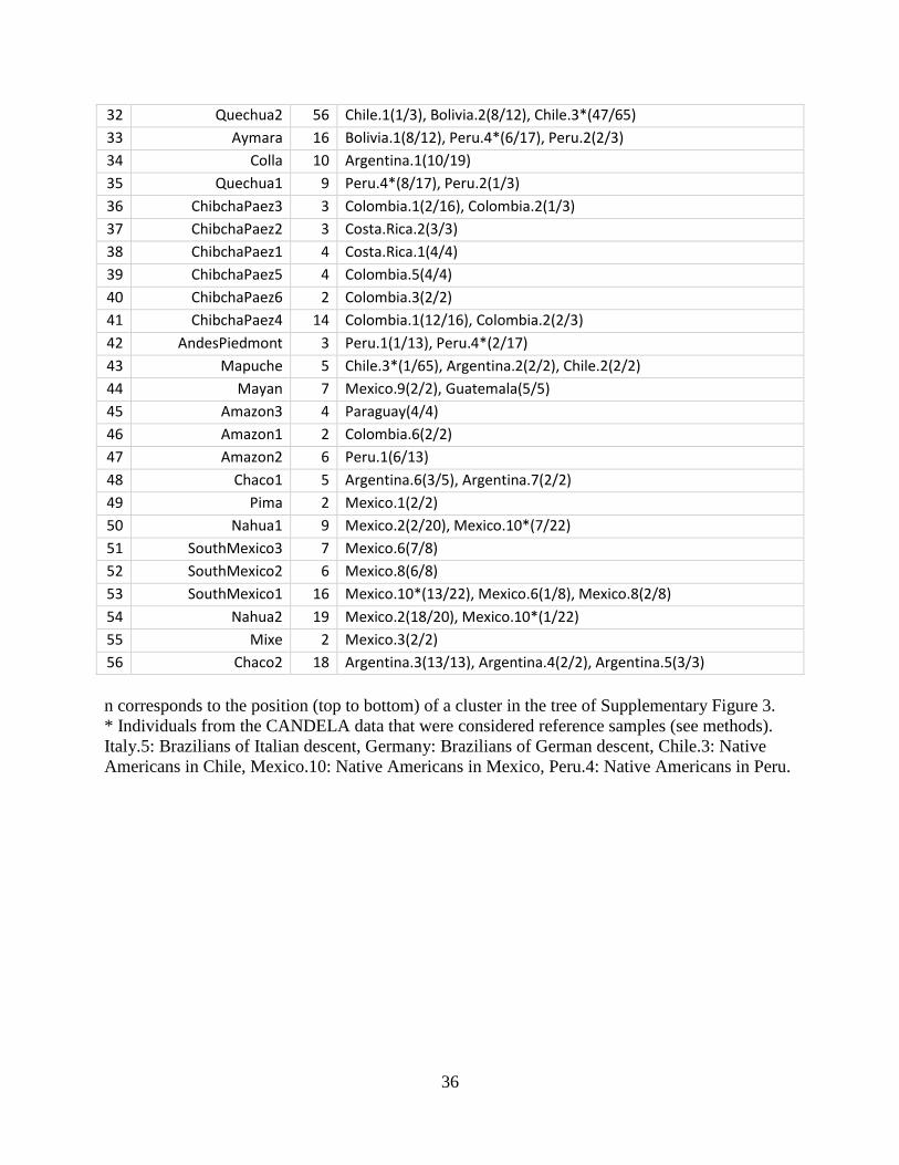
Supplementary Table 3. Individuals from the 117 reference population samples

included in the 56 clusters defined by fineSTRUCTURE

n Cluster label Size Individuals included (labels as in Supplementary Table 1)

1 EastAfrica1 10 Ethiopia(3/3), South.Sudan(7/8)

2 EastAfrica2 73 Kenya(73/73)

3 Namibia 6 Namibia.3(6/9)

4 SouthAfrica 18 South.Africa.3(18/19)

5 WestAfrica1 51 Gambia(51/111)

6 WestAfrica2 68 Sierra.Leone(68/69)

7 WestAfrica3 99 Nigeria.1(99/101)

8 EastMediterranean1 9 Jordan.1(7/15), Yemen(2/2)

9 EastMediterranean2 7 Jordan.1(1/15), Jordan.2(3/3), Palestine(3/3)

10 Sephardic3 7 Morocco.2(7/7)

11 Sephardic1 8 Libya.2(1/7), Turkey.1(7/7)

12 Sephardic2 12 Tunisia.2(6/6), Libya.2(6/7)

13 SouthMediterranean1

28 Tunisia.1(14/14), Libya.1(14/14)

14 SouthMediterranean2

11 Morocco.1(11/11)

15 CentralSouthSpain 48 Spain.2(1/14), Spain.4(13/15), Spain.5(3/4), Spain.6(4/8), Spain.7(4/7), Spain.9(9/12), Spain.10(3/6), Spain.11(5/8), Spain.12(5/14), Spain.14(1/7)

16 CentralNorthSpain 18 Spain.8(1/15), Spain.10(2/6), Spain.12(5/14), Spain.13(5/6), Spain.17(5/6)

17 Catalonia 29 Spain.7(3/7), Spain.12(2/14), Spain.13(1/6), Spain.14(6/7), Spain.15(10/10), Spain.16(7/8)

18 CanaryIslands 18 Spain.2(13/14), Spain.3(2/2), Spain.6(1/8), Spain.11(2/8)

19 Portugal/WestSpain 53 Portugal.1(18/18),Portugal.2(31/31), Spain.1(4/8)

20 Basque 24 Spain.18(14/14), Spain.19(8/8), France.1(2/2)

21 Italy1 19 Italy.5*(15/15), Italy.1(2/2), Bulgaria(2/2)

22 Italy2 31 Italy.3(31/106)

23 NorthWestEurope2 101 NW.Europe(68/91), UK.1(31/31), UK.2(1/29), UK.3(1/1)

24 NorthWestEurope1 31 Germany*(31/37)

25 NorthEastEurope1 2 Russia(2/2)

26 NorthEastEurope2 9 Finland(7/99), Estonia(2/2)

27 NorthEastEurope3 92 Finland (92/99)

28 China/Vietnam1 72 China.1(72/82)

29 China/Vietnam2 91 Vietnam(91/95)

30 ChinaHan 64 China.4(64/101)

31 Japan 103 Japan(103/104)

36

32 Quechua2 56 Chile.1(1/3), Bolivia.2(8/12), Chile.3*(47/65)

33 Aymara 16 Bolivia.1(8/12), Peru.4*(6/17), Peru.2(2/3)

34 Colla 10 Argentina.1(10/19)

35 Quechua1 9 Peru.4*(8/17), Peru.2(1/3)

36 ChibchaPaez3 3 Colombia.1(2/16), Colombia.2(1/3)

37 ChibchaPaez2 3 Costa.Rica.2(3/3)

38 ChibchaPaez1 4 Costa.Rica.1(4/4)

39 ChibchaPaez5 4 Colombia.5(4/4)

40 ChibchaPaez6 2 Colombia.3(2/2)

41 ChibchaPaez4 14 Colombia.1(12/16), Colombia.2(2/3)

42 AndesPiedmont 3 Peru.1(1/13), Peru.4*(2/17)

43 Mapuche 5 Chile.3*(1/65), Argentina.2(2/2), Chile.2(2/2)

44 Mayan 7 Mexico.9(2/2), Guatemala(5/5)

45 Amazon3 4 Paraguay(4/4)

46 Amazon1 2 Colombia.6(2/2)

47 Amazon2 6 Peru.1(6/13)

48 Chaco1 5 Argentina.6(3/5), Argentina.7(2/2)

49 Pima 2 Mexico.1(2/2)

50 Nahua1 9 Mexico.2(2/20), Mexico.10*(7/22)

51 SouthMexico3 7 Mexico.6(7/8)

52 SouthMexico2 6 Mexico.8(6/8)

53 SouthMexico1 16 Mexico.10*(13/22), Mexico.6(1/8), Mexico.8(2/8)

54 Nahua2 19 Mexico.2(18/20), Mexico.10*(1/22)

55 Mixe 2 Mexico.3(2/2)

56 Chaco2 18 Argentina.3(13/13), Argentina.4(2/2), Argentina.5(3/3)

n corresponds to the position (top to bottom) of a cluster in the tree of Supplementary Figure 3.

* Individuals from the CANDELA data that were considered reference samples (see methods).

Italy.5: Brazilians of Italian descent, Germany: Brazilians of German descent, Chile.3: Native

Americans in Chile, Mexico.10: Native Americans in Mexico, Peru.4: Native Americans in Peru.

37

Supplementary Table 4. Regression of Native American ancestry proportion on

inferred admixture date

(A) Analysis Nind Beta se(Beta) t-stat p-value

all 3,340 -1.41 0.14 -10.4 < 1e-15

0.05 < p < 0.95 3,244 -1.56 0.13 -11.7 < 1e-15

0.1 < p < 0.9 3,049 -1.52 0.13 -12.1 < 1e-15

0.2 < p < 0.8 2,534 -1.21 0.11 -11.2 < 1e-15

Simulations (all) 1,297 -0.12 0.17 -1.04 0.30

Simulations, multiple

events (all)

923 -0.11 0.03 -3.73 0.0002

(B) Analysis Nind Beta se(Beta) t-stat p-value

all 3,274 -1.45 0.15 -9.7 < 1e-15

0.05 < p < 0.95 3,189 -1.62 0.14 -11.2 < 1e-15

0.1 < p < 0.9 3,000 -1.60 0.14 -11.8 < 1e-15

0.2 < p < 0.8 2,495 -1.29 0.12 -11.2 < 1e-15

Simulations (all) 1,083 -0.27 0.25 -1.1 0.28

Simulations, multiple

events (all)

832 -0.10 0.04 -2.63 0.009

(A) All individuals. (B) Individuals inferred to have a single date of admixture between 5-17

generations ago.

Inferred coefficients (Beta), standard errors (se(Beta)), t-statistics (t-stat) and p-values for a

simple linear regression of total % Native American ancestry on inferred admixture date, for

individuals inferred to have a single date of admixture between two sources best represented by

European and Native American surrogates. To test robustness, we restricted the regression to

individuals (Nind) whose inferred proportions p of Native and European ancestry each met the

given criterion.

Simulations (all) refers to the simulations described in Supplementary Note 2, section

Simulations with a single admixture event.

Simulations, multiple events (all) refers to the simulations described in Supplementary Note 2,

section Simulations with two sequential admixture events.

38

Supplementary Table 5. Allele frequencies in the Central Andes and the Mapuche at

index SNPs associated with facial features in the CANDELA sample

p-value was calculated using a two-sample t-test.

Allele frequency N (haplotypes)

Chromosomal Region

SNP Gene region Derived Allele

Central Andes

Mapuche Central Andes

Mapuche p-value

2q12 rs3827760 EDAR G 0.961 0.995 879 595 2.60E-06

2q35 rs2395845 PAX3 A 0.388 0.683 896 635 1.35E-31

4q31 rs12644248 DCHS2 G 0.512 0.725 903 699 5.52E-19

6p21 rs1285029 SUPT3H/RUNX2 C 0.585 0.638 880 566 4.46E-02

7p13 rs17640804 GLI3 T 0.417 0.498 892 614 1.85E-03

20p11 rs927833 PAX1 C 0.700 0.503 888 616 1.49E-14

39

Supplementary Table 6. Number of SNPs per GWAS hit matching the criteria to define

the sets of six randomly selected SNPs

Matched

population

rs3827760 rs2395845 rs12644248 rs1285029 rs17640804 rs927833 p-value

CentralAndes

(set I)

32

5656

246

223

2290

5537

0.0176

Mapuche

(set II)

21

1616

94

233

3505

3467

0.0065

Number of SNPs matching the MAF (within <1%) of the given population at each GWAS hit

SNP, and matching the counts (within <20) of inferred Native haplotypes assigned to each of the

Mapuche and Central Andes populations.

SNPs were randomly selected from these matching SNPs to provide 10,000 sets of 6 SNPs, one

matching each GWAS hit SNP, in order to provide an empirical p-value (last column) testing

whether the allele frequencies at the 6 GWAS hit SNPs were more differentiated, on average,

between our assigned Central Andes and Mapuche haplotypes than is typical.

40

Supplementary Table 7. Proportion of Self-copying in Native American surrogate

clusters

Surrogate Self-copying (%) Individuals with >5%

Pima 12.7 3

Nahua1 4.7 1173

Nahua2 29.9 6

SouthMexico1 7.4 963

SouthMexico2 12.7 2

SouthMexico3 28 3

Mixe 63 1

Mayan 3.2 2458

ChibchaPaez1 21.1 320

ChibchaPaez2 28.3 1

ChibchaPaez3 7.8 642

ChibchaPaez4 45.3 1

ChibchaPaez5 16.4 55

ChibchaPaez6 4.4 205

Amazon1 3.1 111

Amazon2 10.8 55

Amazon3 71.4 4

AndesPiedmont 0.8 926

Quechua1 3.1 1474

Aymara 9.6 257

Quechua2 17.9 262

Colla 11.3 66

Mapuche 8.6 1711

Chaco1 5.4 43

Chaco2 26.3 0

Self-copying (%) refers to the average percentage of the genome that all the members of a given

surrogate cluster share within this same cluster according to the coancestry matrix generated by

CHROMOPAINTER. It is an indicator of genetic drift.

Individuals with >5% refers to the number of individuals in the CANDELA dataset with >5%

ancestry, inferred by SOURCEFIND, for that surrogate cluster. Note that highly drifted groups

(i.e. with large self-copying) typically do not show large contributions to CANDELA individuals.

41

Supplementary Table 8. Proportion of inferred admixture events according to

GLOBETROTTER conclusion by different source groups

Source group* n One-date One-date,

multiway

Multiple-

dates, recent

Multiple-

dates, older

Iberia 8167 0.4 0.09 0.24 0.26

INorthWest Europe & Italy 296 0.57 0.15 0.15 0.12

E.Mediterranean & Sephardic 99 0.41 0.04 0.25 0.29

Sub Saharan Africa 1704 0.02 0.28 0.52 0.18

East Asia 87 0.07 0.02 0.89 0.02

ALL SOURCES 3519 455+455** 2378 2378

* The source groups have been defined according to the 56 clusters that were often inferred as

sources by Globetrotter and grouped to represent different historical/demographic processes. In

order to classify an admixture event within a given Source group, the event must have an

admixing source from the corresponding group as a best match at least once.

Iberia includes: CanaryIslands, Portugal/WestSpain, CentralSouthSpain, CentralNorthSpain,

Basque and Catalonia. NorthWestEurope & Italy includes: Italy1 and NorthWestEurope1.

E.Mediterranean & Sephardic includes Sephardic1, EastMediterranean1 and

EastMediterranean2), Sub Saharan Africa includes WestAfrica1, WestAfrica3, EastAfrica1,

EastAfrica2, Namibia and SouthAfrica). East Asia includes Japan, ChinaHan, China/Vietnam1

and China/Vietnam2.

** The two events in this scenario are inferred to be simultaneous.

42

SUPPLEMENTARY NOTES

Supplementary Note 1. ADMIXTURE and Principal Components Analysis (PCA)

The merged dataset was pruned to select SNPs not in Linkage Disequilibrium (LD) using

PLINKv1.9 with the option --indep 50 5 2, resulting in 150,858 SNPs being retained. Supervised

ADMIXTURE analyses were carried out in order to obtain continental ancestry estimates

independent from those obtained with SOURCEFIND. For this, the same reference individuals

included in the SOURCEFIND analyses were grouped into continental reference groups,

considering three scenarios:

A. 5 groups– Native American (NAM), East Asian (EAS), Sub-Saharan African (SSA),

European (EUR) and East/South Mediterranean (ESM)

B. 4 groups – Native American, East Asian, Sub-Saharan African, Caucasian (European +

East/South Mediterranean)

C. 4 groups – Native American, East Asian, Sub-Saharan African, European.

The figure below (Supplementary Figure 15) shows the results for these three scenarios,

with each column depicting the inferred proportion of ancestry the given CANDELA individual

is inferred to match to the 4-5 groups at right:

Supplementary Figure 15. Supervised ADMIXTURE analyses in the CANDELA

43

The figure below (Supplementary Figure 16) compares SOURCEFIND and ADMIXTURE

ancestry estimates across CANDELA individuals for scenario B:

Supplementary Figure 16. Comparison of continental ancestry estimates for the CANDELA sample

obtained with SOURCEFIND and ADMIXTURE

We also applied unsupervised ADMIXTURE and PCA to the same dataset, providing

results for K = 2-10 clusters for ADMIXTURE (Supplementary Fig. 8) and 10PCs for PCA

(Supplementary Fig. 9). Below we describe some major features from these analyses, which are

relevant for the discussion of the SOURCEFIND results.

44

ADMIXTURE analysis (Supplementary Fig. 8) at K = 3 detects three major continental

ancestry components, reaching 100% frequency in certain European, Native American and Sub-

Saharan African reference populations. CANDELA individuals show highly variable proportions

of these three components.

At K = 4, another major continental ancestry component is inferred, reaching 100%

frequency in certain East Asians. This Asian component is found at low frequency in Native

Mexicans and in CANDELA samples from Mexico, possibly reflecting a closer genetic affinity

of Natives from Mexico to East Asians, compared to Native Americans further South, as has

been inferred from other analyses6.

At K = 5 two sub-continental components are detected in Native Americans, one reaching

frequencies of up to 100% in Mesoamericans, the other reaching 100% frequency in Andeans,

with Native populations from Central America and Northern South America showing

intermediate frequencies. The Mesoamerican component reaches high frequency in the Mexican

CANDELA samples and is also the predominant Native component in Colombians. By contrast

the Andean component reaches high frequency in Peruvians and Chileans.

At K=6 a component is seen at high frequency in the Colombian CANDELA data.

Comparing this profile with results for the same CANDELA samples at K=5 it is apparent that

this component corresponds mainly to the inferred European ancestry and possibly reflects

extensive drift in the Colombians (the PCA results described below also provide suggestive

evidence of this interpretation).

At K=7 a third Native American component is observed, reaching 100% frequency in the

Chilean Mapuche Natives. This component reaches high frequency in Chilean CANDELA

samples.

At K = 8 a minor component specific to Sub-Saharan Africans is detected, which reaches

highest frequency in East African samples.

At K = 9 a component reaching frequencies close to 100% in North East Europe is observed.

This component shows a gradient of decreasing frequency from North West Europe to Iberia. It is

also observed in the CANDELA samples, reaching highest frequency in Brazilians.

At K = 10 a component reaching maximum frequencies in Western Europeans is detected,

distinct from a component seen mostly in Southern Europe but which reaches maximum

frequencies in East/South Mediterraneans. These two components are detected at variable

frequencies in the CANDELA samples.

Of the 10 total components at K=10, six reach frequencies close to 100% in certain

reference population groups (from East Asia, Sub-Saharan Africa, North East Europe, the Andes,

Mesoamerica and the Mapuche). Of these, two have a close correspondence with components

defined by the SOURCEFIND analyses (the Mapuche and North East European components).

The other three components detected by ADMIXTURE in the reference data are further sub-

divided by the fineSTRUCTURE analyses. In addition, most ADMIXTURE components show

45

gradients in frequency across many reference samples, which are recognized as distinct

population clusters in the SOURCEFIND analyses (Fig. 1).

Some basic observations from the PCA analyses (Supplementary Fig. 9) are as follows:

PC1-PC3 represent axis of differentiation between continental populations (PC1

distinguishing Africans from Non-Africans, PC2 Europeans from Native Americans and PC3

East Asians from Native Americans). The CANDELA individuals are spread out mostly along

the European-Native American axis, consistent with their mostly Native American-European

admixture. Certain CANDELA individuals also show evidence of some African or East Asian

ancestry.

PCs from PC4 onwards detect sub-continental axis of genetic differentiation. PC4 detecting

genetic variation within Africa and distinguishing West Africans from South Africans.

PC5-PC7 represent axis of differentiation between Native Americans (PC5 corresponding to

a Mexican-Southern Chilean Natives axis.

PC6 to a Mapuche-Chibchan axis and PC7 to a Mapuche-Central Andean axis).

The CANDELA samples place themselves along these axes of Native American variation in

accordance with the Natives from the corresponding geographic region. These observations

illustrate how Native American population structure is being reflected in the CANDELA

samples, a pattern standing out even more clearly in the SOURCEFIND results shown in Figure

1.

Interestingly, the Colombian samples are placed somewhat at an offset along the Chibchan

(i.e. Native Colombians) axis, consistent with the component detected by ADMIXTURE at K = 6

representing a case of drift specific to the Colombian sample.

PC8 corresponds to an axis of South/East Mediterranean-NorthEast European

differentiation.

PC9 to an axis of West African-East African differentiation.

And PC10 to an axis of Japan-China/Vietnam differentiation.

Overall on the first 10 PCs, PCA revealed four axis of continental and six axis of sub-

continental genetic differentiation, placing CANDELA individuals along some of these axes.

From PC11 onwards, there are no discernible patterns of genetic structure.

46

Supplementary Note 2. Assessing the performance of NNLS, SOURCEFIND and

GLOBETROTTER through simulations

Simulations were performed modelling the admixture in Latin America in order to assess the

robustness and accuracy of sub-continental ancestry estimations (NNLS and SOURCEFIND) as

well as the estimated dates of admixture (GLOBETROTTER). Since the precision of sub-

continental ancestry estimates is affected by the relatedness of surrogate clusters, and their level

of genetic drift, these simulations also allowed the exploration of which sub-continental

ancestries cannot be reliably distinguished. Subsets of some of the 56 surrogate clusters were

used to generate simulated admixed individuals following the procedures described in e.g.

Hellenthal et al. 20147 and Price et al. 20098.

The SOURCEFIND approach described in Methods is computationally expensive, due in

part to having to run 50 independent runs in order to sample the parameter space effectively (as

assessed by our simulations). Therefore, for some analyses reported here we used an alternative,

more computationally efficient version of SOURCEFIND that uses the same likelihood function,

but which removes 𝜆 and replaces the prior on the 𝛽𝑟 values with a truncated Poisson (mean=3)

prior on the number of contributing surrogates S'. At each MCMC iteration, this alternative

SOURCEFIND allows only a maximum of S' surrogates to have 𝛽𝑠𝑟 > 0 and for the 𝛽𝑠

𝑟 values of

each of these S' surrogates to be 0.01,…,1 in increments of 0.01. The proposed move at each

MCMC iteration is as follows. Some percentage X<100 𝛽𝑠𝑟 of the current contribution from a

randomly chosen surrogate group s (currently contributing 𝛽𝑠𝑟 > 0) is distributed across the other

currently included surrogates. (This set of other included surrogates contains up to S' members,

with new randomly chosen surrogates added if the total number of surrogates is less than S'.)

With probability 0.1, X = 100 *𝛽𝑠𝑟; otherwise with probability 0.9, X is instead chosen from a

Binomial (n,q) distribution with number of draws n=100*𝛽𝑠𝑟 and probability of each draw q=0.5.

Then with probability 0.5, X/100 is added to the contribution of a single other surrogate;

otherwise it is distributed randomly across the other currently included surrogates. This proposal

is then accepted or rejected using a Metropolis-Hastings step. Here we used S'=6 and performed

100,000 total MCMC iterations, sampling posterior values of 𝛽1𝑟,…, 𝛽𝑆

𝑟 every 5000 iterations

after discarding the initial 50,000 iterations as burn-in. Results under this approach ran much

more quickly and gave qualitatively similar conclusions in applications to simulated and non-

simulated data, as described in this section and Supplementary Note 6.

In particular in each of simulations (i)-(iv) described below, we provide plots illustrating the

accuracy of both the initial SOURCEFIND version (called SOURCEFIND1 in this section) and

the computationally efficient version of SOURCEFIND (called SOURCEFIND2). For these

simulations, accuracy is only very slightly reduced when using SOURCEFIND2 relative to

SOURCEFIND1. Regarding computation time, analysis of a single CANDELA individual took

~10 minutes using each run of the initial SOURCEFIND version with 200K MCMC iterations,

hence taking 10x50=500 minutes to do 50 independent runs. In contrast, it took ~25 seconds with

100K MCMC iterations and a single run of the more computationally efficient version. We note

that additional independent runs of the computationally efficient version may improve

performance, while reducing the gains in computation time (e.g. doing 50 independent runs

would make it only ~20x faster than the initial SOURCEFIND). The computationally efficient

version of SOURCEFIND is available at www.paintmychromosomes.com.

47

Simulations to assess the accuracy of sub-continental ancestry estimates

For each set of simulations in this section, we generated 100 simulated individuals as

mixtures of three surrogate clusters intermixing 15 generations ago. From the clusters selected for

the simulations, we used less than half the individuals in a cluster to simulate admixed

individuals. The remaining individuals in a cluster were used for the

CHROMOPAINTER/SOURCEFIND inference. Simulations were as described in Price et al.

20098 and assume a model of instantaneous admixture followed by random mating among the

admixed individuals. Briefly, each simulated haploid genome consists of a mosaic of blocks, with

each block of size M (in Morgans) sampled from an exponential distribution (of rate=15). For

each block, the SNP data exactly matched that of a randomly sampled haplotype from one of the

surrogate clusters, with the probabilities for selecting a haplotype from each of the three surrogate

clusters specified by the admixture proportions being simulated as indicated below. This random

selection process was repeated independently for each block. Two haploid genomes were

randomly combined to generate each simulated diploid individual.

SOURCEFIND1 analyses were performed with 20 independent runs using 200,000

iterations each run as described in methods, with SOURCEFIND2 analyses run as described in

the previous section. NNLS was performed using the procedure encoded in GLOBETROTTER

described in Hellenthal et al. 20147, which uses the non-negative linear least squares function

(nnls) in R. As with the real data analysis, for each run results with highest posterior probability

values were chosen, averaging inferred ancestry proportions across the 20 runs using this

probability as a weight. We note that accuracy of both NNLS and SOURCEFIND depends in part

on the number of individuals used in each surrogate group, so that removing ~30% of the

individuals from each simulating group when performing inference may decrease accuracy.

Four sets of simulations with different admixture percentages were performed and these are

described below. The values in parenthesis indicate the fraction of individuals from a cluster that

were used to generate the admixed individuals in that simulation.

(i) 40% CentralSouthSpain (16/48), 30% NorthWestEurope2 (32/101), 30% SouthMexico1

(5/16)

When using NNLS as described in e.g. Leslie et al. 20159, ancestry from SouthMexico1 is

inferred with high accuracy, showing little marginal uncertainty and little misassignment even to

Nahua1, a striking result considering that these two surrogate clusters are closely related as

shown in the fineSTRUCTURE tree (Supplementary Fig. 3). The accuracy obtained with

SOURCEFIND1/SOURCEFIND2 is even higher, having a nearly perfect match to the true

simulated proportions and sources.

The following pyramid chart in Supplementary Figure 17 (and those for the next three sets

of simulations) shows the distribution of simulated ancestry proportions from each surrogate

cluster across the 100 simulated individuals. Colours correspond to major geographic regions:

48

NAM (blue), EUR (red), ESM (dark orange), SSA (green), and EAS (purple). Black horizontal

lines show the mean proportions of ancestry from each source group.

Supplementary Figure 17. Pyramid charts showing the distribution of simulated ancestry proportions

from each surrogate cluster across the 100 simulated individuals for scenario (i)

In the case of CentralSouthSpain, NNLS shows high levels of misassignment to other

Iberian surrogates. The highest missassigned values are to CentralNorthSpain, which is the group

49

genetically most similar to CentralSouthSpain. Additional contributions are inferred for

East/South Mediterranean populations (up to ~5%). In contrast, SOURCEFIND estimations are

highly accurate, with very minor inferred incorrect contributions related to Italy1. Importantly,

there are no mis-inferred contributions from East/South Mediterranean populations when using

SOURCEFIND.

The estimation of NorthWestEurope2 ancestry is typically more accurate, with some

incorrect assignment to NorthWestEurope1 (max ~10%), that is considerably stronger under

NNLS.

Overall, this simulation demonstrates the increased resolution of SOURCEFIND compared

to NNLS for resolving ancestral origins among Iberian populations. SOURCEFIND also has

reduced mis-specified contributions related to East/South Mediterranean groups.

(ii) 40% Portugal/WestSpain (16/53), 30% Italy1 (7/19), 30% Aymara (6 /16)

NNLS analysis results in a poor discrimination of Aymara from Quechua2 ancestry,

consistent with the high genetic similarity of these two groups and the small size for the Aymara

cluster (n=16). We note that when Quechua2 ancestry is included in the simulations instead of

Aymara (simulation iii below) higher accuracy is obtained, showcasing the increased accuracy

when using more surrogate individuals from the admixing group when performing inference. In

the case of the SOURCEFIND analysis, both Aymara and Quechua2 ancestries are accurately

estimated under both simulation scenarios.

Both NNLS and SOURCEFIND slightly overestimate the Portugal/WestSpain contribution

and slightly underestimate the ancestry from Italy1. However, SOURCEFIND inferences are

closer to the simulated proportions than those of NNLS. Furthermore, as in the previous

simulation, NNLS infers East/South Mediterranean contributions, as well as several other

incorrect European contributions, which are not inferred in the SOURCEFIND analyses.

50

Supplementary Figure 18. Pyramid charts showing the distribution of simulated ancestry proportions

from each surrogate cluster across the 100 simulated individuals for scenario (ii)

51

(iii) 40% Quechua2 (15/56), 40% CentralSouthSpain (16/48), 20% WestAfrica3 (22/99)

Estimated contributions from WestAfrica3 and Quechua2 are very accurate under both

NNLS and SOURCEFIND, with the latter again showing more accurate estimates overall. We

note that NNLS infers a notable spurious contribution from Basque, which suggests that inferred

Basque-like contributions in the Americas using this approach should be treated with caution10.

Supplementary Figure 19. Pyramid charts showing the distribution of simulated ancestry proportions

from each surrogate cluster across the 100 simulated individuals for scenario (iii)

52

(iv) 40% SouthMexico1 (6 /16), 40% Mayan (3/7), 20% CentralSouthSpain (16/48)

Supplementary Figure 20. Pyramid charts showing the distribution of simulated ancestry proportions

from each surrogate cluster across the 100 simulated individuals for scenario (iv)

53

These simulation results suggest that, for NNLS, the presence of different mis-specified

signals of ancestry across the Iberian groups may be proportional to the amount of true ancestry

from these sources, which could allow the establishment of noise thresholds in NNLS inference.

For example, if the highest values of Basque ancestry in an individual with 20%

CentralSouthSpain is around 2% for simulations here, and around 4% for an individual with 40%

CentralSouthSpain (see simulation set (iii)), we could in theory predict that an individual in the

real dataset with 80% CentralSouthSpain-like ancestry may have ~8% Basque ancestry

attributable to noise. SOURCEFIND does not show this problem, instead showing only a slight

mis-assignment of this Iberian component to the closest group (CentralNorthSpain).

The two Native American components, although closely related, are distinguishable by both

approaches, although SOURCEFIND shows greater precision.

Simulations to assess the accuracy of per individual estimation of time since admixture and

the effect of time since admixture on ancestry estimation

Simulations with a single admixture event

We simulated an additional 1,430 individuals with different proportions of admixture from

two sources (CentralSouthSpain and Quechua2) and different times since admixture. Using the

procedure described in the previous section, each individual was simulated as descending from an

instantaneous admixture event that occurred g generations ago, with a proportion p of ancestry

from CentralSouthSpain, and 1-p ancestry from Quechua2. We simulated p = 0.05, 0.1, 0.2, 0.3,

0.4, 0.5, 0.6, 0.7, 0.8, 0.9, 0.95 and g = 5-17 generations, with 10 simulated individuals for each

combination of p and g, resulting in a total of 1,430 simulated individuals.

We used 16 CentralSouthSpain and 20 Quechua2 individuals to generate the admixed

individuals, using the remaining 32 CentralSouthSpain and 36 Quechua2 individuals to infer

ancestry using SOURCEFIND and GLOBETROTTER. SOURCEFIND and GLOBETROTTER

were run separately on each simulated individual as described for the real data samples, with the

slight modification that GLOBETROTTER was allowed to use all surrogates to describe the

admixture (rather than only including surrogates inferred by SOURCEFIND to contribute >1%).

In contrast to the simulations above, for these simulations we used the more computationally

efficient version of SOURCEFIND (i.e. SOURCEFIND2), described at the start of this

Supplementary Note, to infer proportions.

The figure below (Supplementary Figure 21) shows that on average, GLOBETROTTER’s

individual estimated dates accurately reflect the simulated dates (grey bar), and that this accuracy

is not affected by variation in the admixture proportions (the figure has been produced with the

default parameters of the function boxplot.default in R: The centre line corresponds to the

median, the bounds of box represent the first (𝑄1) and the third (𝑄3) quartiles, and the whiskers

approximate to 𝑄1 - 1.5*Inter-Quartile Range and 𝑄3 + 1.5*Inter-Quartile Range. Outlying points

are plotted individually).

54

Supplementary Figure 21. GLOBETROTTER’s inferred dates (y-axis) across individuals, for simulations

mixing CentralSouthSpain and Quechua2 at the given proportions (legend) and times (x-axis)

Similarly, the figure below shows that SOURCEFIND’s accuracy in inferring ancestry

proportions in the simulated individuals did not depend on the date of admixture (simulated

proportions highlighted with a grey bar).

Supplementary Figure 22. SOURCEFIND's inferred proportion of ancestry related to Iberian (IBR) and

Native American (NAM) sources (y-axis) across individuals (circles), for simulations mixing

CentralSouthSpain and Quechua2 at the given proportions (x-axis) and times (legend)

55

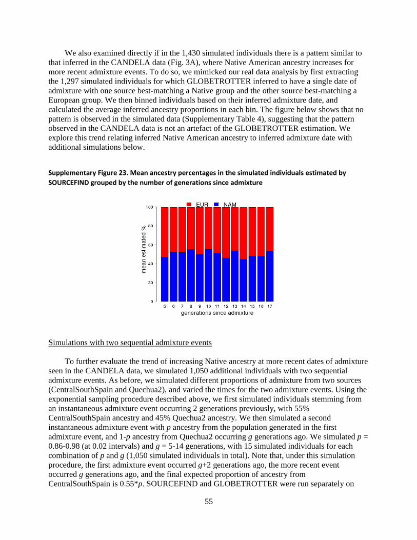
We also examined directly if in the 1,430 simulated individuals there is a pattern similar to

that inferred in the CANDELA data (Fig. 3A), where Native American ancestry increases for

more recent admixture events. To do so, we mimicked our real data analysis by first extracting

the 1,297 simulated individuals for which GLOBETROTTER inferred to have a single date of

admixture with one source best-matching a Native group and the other source best-matching a

European group. We then binned individuals based on their inferred admixture date, and

calculated the average inferred ancestry proportions in each bin. The figure below shows that no

pattern is observed in the simulated data (Supplementary Table 4), suggesting that the pattern

observed in the CANDELA data is not an artefact of the GLOBETROTTER estimation. We

explore this trend relating inferred Native American ancestry to inferred admixture date with

additional simulations below.

Supplementary Figure 23. Mean ancestry percentages in the simulated individuals estimated by

SOURCEFIND grouped by the number of generations since admixture

Simulations with two sequential admixture events

To further evaluate the trend of increasing Native ancestry at more recent dates of admixture

seen in the CANDELA data, we simulated 1,050 additional individuals with two sequential

admixture events. As before, we simulated different proportions of admixture from two sources

(CentralSouthSpain and Quechua2), and varied the times for the two admixture events. Using the

exponential sampling procedure described above, we first simulated individuals stemming from

an instantaneous admixture event occurring 2 generations previously, with 55%

CentralSouthSpain ancestry and 45% Quechua2 ancestry. We then simulated a second

instantaneous admixture event with p ancestry from the population generated in the first

admixture event, and 1-p ancestry from Quechua2 occurring g generations ago. We simulated p =

0.86-0.98 (at 0.02 intervals) and g = 5-14 generations, with 15 simulated individuals for each

combination of p and g (1,050 simulated individuals in total). Note that, under this simulation

procedure, the first admixture event occurred g+2 generations ago, the more recent event

occurred g generations ago, and the final expected proportion of ancestry from

CentralSouthSpain is 0.55*p. SOURCEFIND and GLOBETROTTER were run separately on

56

each simulated individual as before. As with the previous section, for these simulations we used

the more computationally efficient version of SOURCEFIND (i.e. SOURCEFIND2), described at

the start of this Supplementary Note, to infer proportions.

In 923 (~88%) of the 1,050 individuals, GLOBETROTTER concluded only a single date of

admixture, which is not surprising given the inherent difficulty in distinguishing between two

pulses of admixture separated by only 2 generations that involve the same source groups. The

figure below (Supplementary Figure 24) shows results when assuming a single date of admixture,

which infers dates that typically are 2 generations above g (simulated date given with the grey

bar). Therefore, GLOBETROTTER most often concludes a single date of admixture, with the

inferred date primarily reflecting the older event because this is reflected in the sizes of observed

Iberian ancestry segments (the figure has been produced with the default parameters of the

function boxplot.default in R as explained in the previous section).

Supplementary Figure 24. GLOBETROTTER’s inferred dates (y-axis) across individuals, for simulations

with two sequential admixture events, at the given proportions (legend) and times (x-axis).

The figure below (Supplementary Figure 25) illustrates that SOURCEFIND accurately

estimates the admixture proportions in the simulated individuals (grey bar gives simulated

proportion).

57

Supplementary Figure 25. SOURCEFIND's inferred proportion of ancestry related to Iberian (IBR) and

Native American (NAM) sources (y-axis) across individuals (circles), for simulations with two sequential

admixture events, at the given proportions (x-axis) and times (legend).

In addition, as above, we extracted the 923 simulated individuals that GLOBETROTTER

inferred to have a single admixture event between source groups that best-matched Native and

European surrogate groups. We binned these individuals based on their inferred admixture date,

and calculated the average ancestry inferred proportions in each bin. While not as striking as that

observed in our real data (Fig. 3A of the main text), the figure below shows an analogous trend

for decreasing Native American ancestry at increasing g that is significant (p<0.001) under the

same simple linear regression model used for analysing this trend in the real data (Supplementary

Table 4). This is because individuals here are simulated with different proportions of admixture

from the earlier admixture event occurring g+2 generations ago. Individuals with more simulated

ancestry from this earlier admixed group have (i) more European ancestry and (ii) inferred dates

that may be slightly older by retaining more signal from this older admixture event. Indeed, a

simple linear regression of the bias in date estimate (in generations ago) for these 923 individuals

on their expected proportion of Spanish ancestry shows a significantly positive association

(p<0.007). In contrast, for the 1,297 simulated individuals described in the previous section with

only a single simulated admixture date, there is no such significant trend (p=0.33). Overall these

simulation results suggest that mixture between unadmixed and admixed Natives over time, such

as that we simulated in this section, could lead to the trend we observe in Figure 3A.

58

Supplementary Figure 26. Mean ancestry percentages in the simulated individuals for two sequential

admixture events estimated by SOURCEFIND, grouped by the number of generations since admixture.

Assessing the reliability of East/South Mediterranean ancestry estimation

The simulations above do not include East/South Mediterranean (ESM) ancestry. We can

therefore use them to assess the amount of spurious ESM ancestry inferred in our analyses. For

the 400 individuals described in the first section of this Supplementary Note, where the

proportion of simulated Iberian ancestry ranges from 20-40%, SOURCEFIND estimates that

none of these have >1% ESM ancestry. Across all simulations (2,880 individuals), only 2

(~0.07%) had >5% ESM ancestry (maximum = 6.2%, with both of these 2 simulated individuals

having >90% Iberian ancestry, and 72 (2.5%) had inferred ESM ancestry >2%. In the main text,

we note that ~23% of CANDELA individuals are inferred by SOURCEFIND to have >5% ESM

ancestry (Fig. 1E). Furthermore, in the CANDELA data, 878 (~14.6%) individuals are inferred to

have >10% ESM ancestry, an amount never inferred in any of the simulations performed (even in

individuals with 90% simulated Iberian ancestry). The simulation results are therefore consistent

with ancestors of these Latin American individuals having substantially greater ESM ancestry

than the present Iberian groups sampled.

59

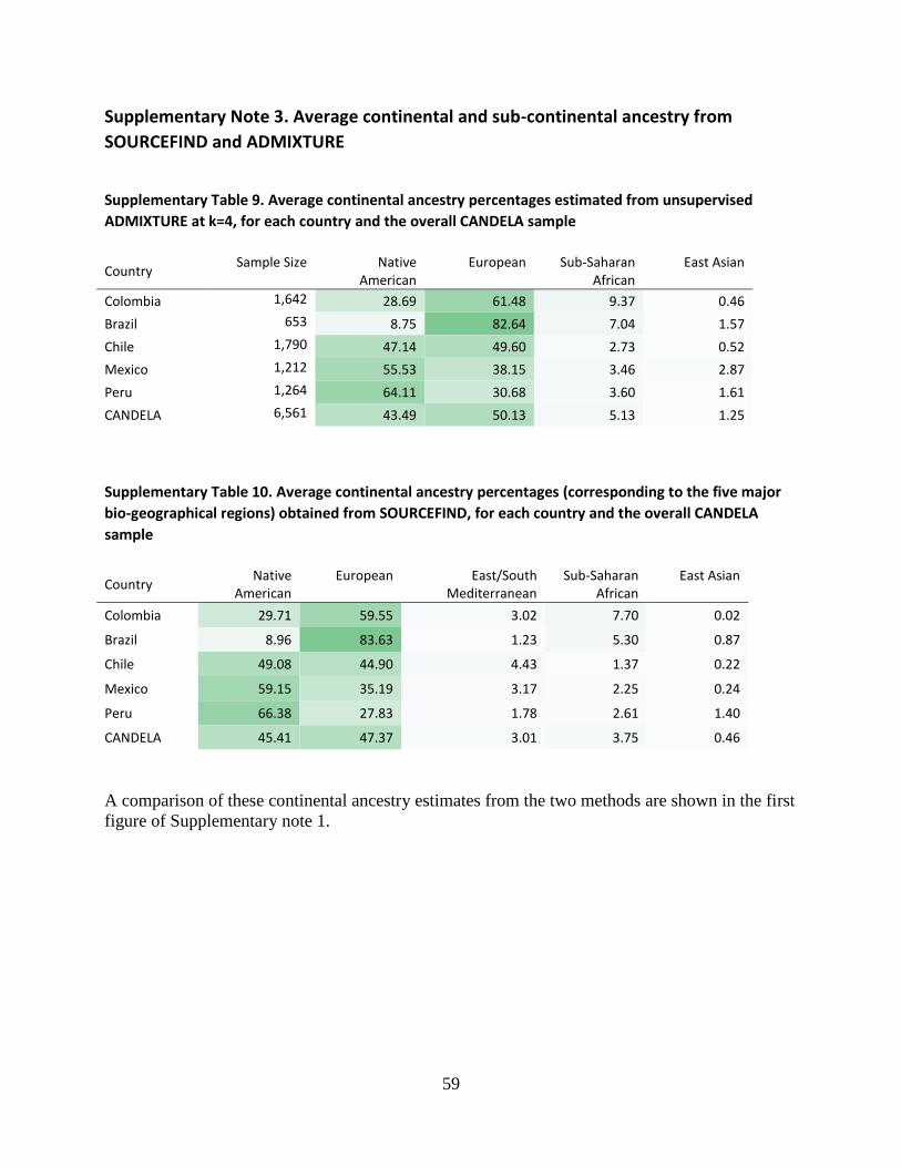
Supplementary Note 3. Average continental and sub-continental ancestry from

SOURCEFIND and ADMIXTURE

Supplementary Table 9. Average continental ancestry percentages estimated from unsupervised

ADMIXTURE at k=4, for each country and the overall CANDELA sample

Country Sample Size Native

American European Sub-Saharan

African East Asian

Colombia 1,642 28.69 61.48 9.37 0.46

Brazil 653 8.75 82.64 7.04 1.57

Chile 1,790 47.14 49.60 2.73 0.52

Mexico 1,212 55.53 38.15 3.46 2.87

Peru 1,264 64.11 30.68 3.60 1.61

CANDELA 6,561 43.49 50.13 5.13 1.25

Supplementary Table 10. Average continental ancestry percentages (corresponding to the five major

bio-geographical regions) obtained from SOURCEFIND, for each country and the overall CANDELA

sample

Country Native

American European East/South

Mediterranean Sub-Saharan

African East Asian

Colombia 29.71 59.55 3.02 7.70 0.02

Brazil 8.96 83.63 1.23 5.30 0.87

Chile 49.08 44.90 4.43 1.37 0.22

Mexico 59.15 35.19 3.17 2.25 0.24

Peru 66.38 27.83 1.78 2.61 1.40

CANDELA 45.41 47.37 3.01 3.75 0.46

A comparison of these continental ancestry estimates from the two methods are shown in the first

figure of Supplementary note 1.

60

Supplementary Table 11. Average sub-continental ancestry percentages (for the 35 groups) obtained

from SOURCEFIND, for each country and the overall CANDELA sample

Group Colombia Brazil Chile Mexico Peru CANDELA

Native American

Pima 0.00 0.00 0.00 0.02 0.00 0.00

Nahua1 0.08 0.05 0.00 44.10 0.02 8.18

Nahua2 0.00 0.00 0.00 0.09 0.00 0.02

SouthMexico 0.01 0.03 0.00 12.38 0.00 2.29

Mixe 0.00 0.00 0.00 0.01 0.00 0.00

Mayan 8.89 1.53 0.09 2.28 0.23 2.87

ChibchaPaez 13.91 0.11 0.00 0.04 0.01 3.50

Amazon 0.10 0.62 0.00 0.00 0.14 0.12

AndesPiedmont 6.70 6.13 3.01 0.22 26.71 8.27

Quechua1 0.00 0.24 4.81 0.03 33.27 7.72

Aymara 0.00 0.00 2.90 0.00 5.30 1.81

Quechua2 0.00 0.00 6.11 0.00 0.62 1.79

Colla 0.00 0.00 0.22 0.00 0.00 0.06

Mapuche 0.01 0.06 31.92 0.00 0.08 8.75

Chaco1 0.00 0.18 0.00 0.00 0.00 0.02

Chaco2 0.00 0.00 0.00 0.00 0.00 0.00

European

CanaryIslands 4.68 2.94 1.36 1.94 0.92 2.37

Portugal/WestSpain 8.76 42.59 2.85 3.89 2.63 8.45

CentralSouthSpain 36.01 1.17 36.31 24.77 19.05 27.28

CentralNorthSpain 8.79 0.29 2.55 2.96 2.94 4.03

Basque 0.45 0.03 0.09 0.18 0.19 0.21

Catalonia 0.51 1.40 0.63 0.65 1.12 0.77

Italy 0.24 18.28 0.86 0.43 0.79 2.35

NorthWestEurope 0.09 15.89 0.25 0.28 0.18 1.77

NorthEastEurope 0.02 1.04 0.02 0.09 0.02 0.13

East/South Mediterranean

Sephardic 2.29 0.36 2.43 1.60 1.14 1.79

EastMediterranean 0.51 0.80 1.60 1.22 0.47 0.96

SouthMediterranean 0.21 0.07 0.39 0.35 0.17 0.26

Sub-Saharan African

WestAfrica 6.71 3.55 1.01 1.89 2.30 3.10

EastAfrica 0.75 1.04 0.27 0.30 0.22 0.46

Namibia 0.08 0.30 0.04 0.03 0.02 0.07

SouthAfrica 0.16 0.41 0.05 0.04 0.06 0.12

East Asian

Japan 0.00 0.72 0.02 0.08 0.30 0.15

ChinaHan 0.01 0.13 0.13 0.07 0.76 0.21

China/Vietnam 0.01 0.02 0.07 0.09 0.34 0.11

61

Supplementary Note 4. Definition of the phenotypes examined in Figure 4

- Height. Quantitative measurement (in cm).

Scalp and face hair:

- Monobrow and Eyebrow density (in men). 1: low, 2: medium or 3: high (thinner to thicker).

- Beard density (in men). 1: low, 2: medium or 3: high.

- Scalp hair shape. 1: straight, 2: wavy, 3: curly or 4: frizzy.

- Scalp hair greying. 1: no greying, 2: predominant no greying, 3: 50% greying, 4: predominant

greying or 5: totally white hair.

- Balding (Measured in men and women). 1: low, 2: medium or 3: high.

Pigmentation:

- Natural hair colour. 1: blond, 2: dark blond/light brown or 3: brown/black.

- Skin colour (Melanin index). Quantitative measurement using DermaSpectrometer DSMEII

reflectometer (Cortex Technology, Hadsund, Denmark). The value used for each individual

corresponds to the mean index for both inner arms.

- Eye color. 1: blue/grey, 2: Honey, 3: Green, 4: light brown, 5: dark brown/black.

Categorical face traits:

- Brow ridge protrusion. The presence and degree of a ridge in lateral view. 0: none, 1: slightly

pronounced or 2: strongly pronounced.

- Eye fold. Skin fold of the upper eyelid, covering the inner corner (medial canthus) of the eye. 0:

no fold, 1: partial, 2: completely.

- Chin shape. Chin contour in frontal view. 0: pointed, 1: rounded or 2: square.

Quantitative face traits:

These were defined based on landmarks placed on facial photographs as detailed in the figure

below:

Supplementary Figure 27. Landmarks placed on facial photographs obtained for CANDELA.

This figure is modified from Adhikari et al. 201611

62

- Forehead profile. Slope of line joining 35-1.

- Nasion position. Distance from landmark 18 to the mid-point of a line joining landmarks 8 and

16.

- Nose bridge breadth. Distance between landmarks 37 and 38.

- Nose wing breadth. Distance between landmarks 20 and 22.

- Columella Inclination. Angle between landmarks 19-21-23

- Nose protrusion. Distance of landmark 19 to a line joining landmarks 18 and 21

- Nose tip angle. Angle between landmarks 18-19-21.

- Chin protrusion. Distance of point 30 from line joining 35-36.

- Facial flatness. Distance 30-32/ distance 32-18.

Ear traits:

The location of these features is shown in the photographs below. All traits were ordinal and

scored on a 3-point scale (low, medium, high).

Supplementary Figure 28. Ear traits characterized in the CANDELA dataset.

This figure is modified from Adhikari et al. 201512

- Ear protrusion. Degree of protrusion of the ear in relation to the frontal face view (less to more

protruded).

- Lobe attachment. Degree of attachment of the inferior part of the pinna to the anteroinferior part

of the face (no attached to completely attached).

- Lobe size. Small to bigger size.

- Helix rolling. The outer rim of the ear that extends from the superior insertion of the ear on the

scalp (root) to the termination of the cartilage at the earlobe (less to more pronounced helix

rolling).

- Fold of antihelix. Less to more pronounced fold of antihelix.

- Antitragus size. Small to bigger size. The anterosuperior cartilaginous protrusion lying between

the incisura and the origin of the antihelix. The anterosuperior margin of the antitragus forms the

posterior wall of the incisura.

More information on these phenotypes can be found in previous CANDELA papers11-14.

63

Supplementary Note 5. Correlation of regression p-values from different approaches to

the Central Andes - Mapuche ancestry contrast

Regression analyses for testing the phenotypic effect of the contrast between Central Andes and

Mapuche ancestry were performed using three different approaches to define these ancestry

components, based on the SOURCEFIND, ADMIXTURE, or PCA (Supplementary Figures 8

and 9).

● SOURCEFIND: estimates of the Aymara, Quechua1, Quechua2, and Colla components were

added and the sum (taken as the Central Andes component) contrasted to the Mapuche

component. Regressions were performed in three ways: (i) including individuals from all

countries, (ii) including only Peruvians and Chileans (both the Central Andes and Mapuche

components are only present in these two countries, Fig. 1), (iii) including only Chileans (as

only this country has both the Central Andes and the Mapuche components at high frequency,

Figure 1).

● ADMIXTURE: the unsupervised run at K=7 distinguishes three components in Native

Americans (Supplementary Fig. 8). A light-blue colored component reaches 100% frequency

in the Central Andean groups while a grey colored component reaches 100% frequency in the

Mapuche. The difference in the proportions of these two ancestry components was taken as

the Central Andes - Mapuche contrast. Regression analysis was performed including

individuals from all countries.

● PCA: PC7 places Central Andean and Mapuche clusters at opposite ends (Supplementary Fig.

9). Individual values on this PC were taken directly as an approximation to the contrast

between these two components. However, since this PC shows some confounding with other

ancestry differences, the regression included only Chileans (as these individuals have a

relatively low frequency of other Native American ancestry components, Fig. 1,

Supplementary Fig. 8).

Below are Spearman’s rank correlations calculated between the -log p-values obtained in the

regressions described above (Sample sizes: all individuals N = 5794, Peruvians and Chileans N =

2594, Chileans N = 1542).

Supplementary Table 12. Spearman’s rank correlations

ADMIXTURE SOURCEFIND

(all individuals) SOURCEFIND

(Peruvians and Chileans)

SOURCEFIND (Chileans)

PCA

ADMIXTURE 1.00 0.94 0.83 0.92 0.90

SOURCEFIND (all individuals)

0.94 1.00 0.83 0.91 0.88

SOURCEFIND (Peruvians and Chileans)

0.83 0.83 1.00 0.92 0.84

SOURCEFIND (Chileans) 0.92 0.91 0.92 1.00 0.92

PCA 0.90 0.88 0.84 0.92 1.00

64

Supplementary Note 6. Robustness of SOURCEFIND ancestry inference to the exclusion

CANDELA individuals used as reference samples

To assess the impact of having included some CANDELA individuals as reference samples

in the SOURCEFIND analyses, we repeated our analyses after excluding CANDELA individuals

from the reference samples. We also removed individuals that were excluded from the surrogate

groups as described in methods (Definition of homogeneous clusters of reference population

individuals), resulting in this analysis including only 55 surrogate clusters. The loss of one

surrogate cluster relative to the initial analyses was due to the Germany surrogate cluster

consisting entirely of CANDELA individuals. As described at the start of Supplementary Note 2,

for this analysis we used an alternative, more efficient version of SOURCEFIND (i.e.

SOURCEFIND2) that used a truncated Poisson prior on the number of contributing surrogates

and allowed a maximum of 6 surrogates to contribute at each MCMC iteration.

Maps with the distribution of the new estimated individual ancestry proportions are shown

below. Ancestry matching to European, East/South Mediterranean, Sub-Saharan African, and

East Asian groups are largely consistent with the results shown in Figure 2. For Native American

ancestry, results are similar across most of the CANDELA sample. However there is a marked

decrease in inferred ancestry related to the AndesPiedmont and Quechua1 surrogate groups. This

is probably due to these groups being made up of only one individual, after removal of

CANDELA samples, thus decreasing the power of ancestry inference from these groups. The

inferred ancestry contributions of these groups are, for the most part, substituted by ancestries

from related, geographically proximate, surrogate groups.

Supplementary Figure 29. Individual pie-maps showing SOURCEFIND analyses when not including any

CANDELA reference samples as surrogates or donors.

65

References

1. Mallick, S. et al. The Simons Genome Diversity Project: 300 genomes from 142 diverse

populations. Nature 538, 201-206 (2016).

2. Eichstaedt, C.A. et al. The Andean adaptive toolkit to counteract high altitude

maladaptation: genome-wide and phenotypic analysis of the Collas. PLoS One 9, e93314

(2014).

3. 1000 Genomes Project, C. A global reference for human genetic variation. Nature 526,

68-74 (2015).

4. Pagani, L. et al. Ethiopian genetic diversity reveals linguistic stratification and complex

influences on the Ethiopian gene pool. Am J Hum Genet 91, 83-96 (2012).

5. Schlebusch, C.M. et al. Genomic variation in seven Khoe-San groups reveals adaptation

and complex African history. Science 338, 374-9 (2012).

6. Reich, D. et al. Reconstructing Native American population history. Nature 488, 370-4

(2012).

7. Hellenthal, G. et al. A genetic atlas of human admixture history. Science 343, 747-51

(2014).

8. Price, A.L. et al. Sensitive detection of chromosomal segments of distinct ancestry in

admixed populations. PLoS Genet 5, e1000519 (2009).

9. Leslie, S. et al. The fine-scale genetic structure of the British population. Nature 519,

309-14 (2015).

10. Montinaro, F. et al. Unravelling the hidden ancestry of American admixed populations.

Nat Commun 6, 6596 (2015).

11. Adhikari, K. et al. A genome-wide association scan in admixed Latin Americans

identifies loci influencing facial and scalp hair features. Nat Commun 7, 10815 (2016).

12. Adhikari, K. et al. A genome-wide association study identifies multiple loci for variation

in human ear morphology. Nat Commun 6, 7500 (2015).

13. Adhikari, K. et al. A genome-wide association scan implicates DCHS2, RUNX2, GLI3,

PAX1 and EDAR in human facial variation. Nat Commun 7, 11616 (2016).

14. Ruiz-Linares, A. et al. Admixture in Latin America: geographic structure, phenotypic

diversity and self-perception of ancestry based on 7,342 individuals. PLoS Genet 10,

e1004572 (2014).