Embed Size (px)
Citation preview
Part III
Open MacroeconomicSystems of Debt Money
301

Chapter 10
Balance of Payments andForeign Exchange
This chapter1 explores a dynamic determination process of foreign exchangerate in an open macroeconomy in which goods and services are freely traded andfinancial capital flows efficiently for higher returns. For this purpose it becomesnecessary to employ a new method contrary to a standard method of dealingwith a foreign sector as adjunct to macroeconomy; that is, an introduction ofanother macroeconomy as a foreign sector. Within this new framework of openmacroeconomy, transactions among domestic and foreign sectors are handledaccording to the principle of accounting system dynamics, and their balance ofpayments is attained. For the sake of simplicity of analyzing foreign exchangedynamics, macro variables such as GDP, its price level and interest rate aretreated as outside parameters. Then, eight scenarios are produced and examinedto see how exchange rate, trade balance and financial investment, etc. respondto such outside parameters. To our surprise, expectations of foreign exchangerate turn out to play a crucial role for destabilizing trade balance and financialinvestment. The impact of official intervention on foreign exchange and a pathto default is also discussed.
10.1 Open Macroeconomy as a Mirror Image
As a natural step of the research, we are now in a position to open our macroe-conomy to a foreign sector so that goods and services are freely traded and fi-nancial assets are efficiently invested for higher returns. The analytical methodemployed here is the same as the previous chapters; that is, the one based onthe principle of accounting system dynamics.
1It is based on the paper: Balance of Payments and Foreign Exchange Dynamics – SDMacroeconomic Modeling (4) – in “Proceedings of the 24th International Conference of theSystem Dynamics Society”, Boston, USA, July 29 - August 2, 2007. (ISBN 978-0-9745329-8-1)
304CHAPTER 10. BALANCE OF PAYMENTS AND FOREIGN EXCHANGE
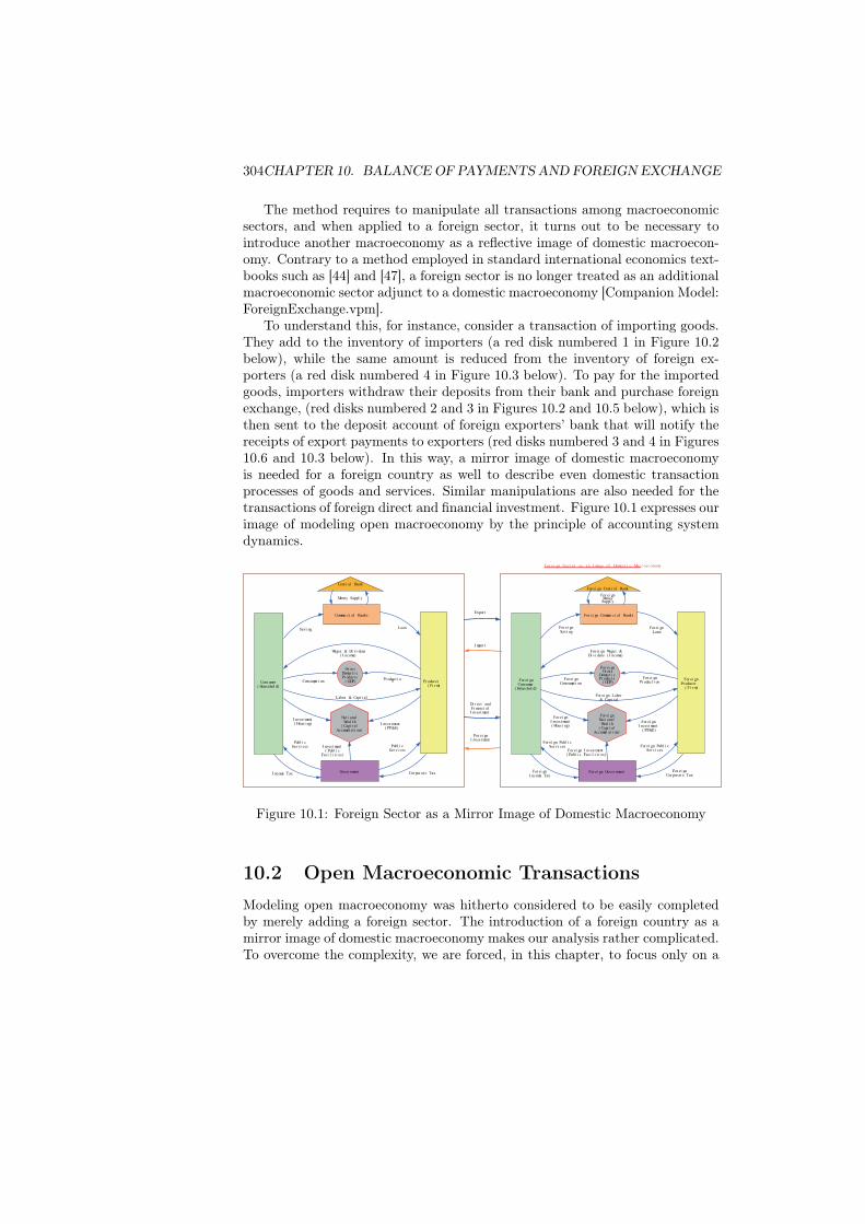
The method requires to manipulate all transactions among macroeconomicsectors, and when applied to a foreign sector, it turns out to be necessary tointroduce another macroeconomy as a reflective image of domestic macroecon-omy. Contrary to a method employed in standard international economics text-books such as [44] and [47], a foreign sector is no longer treated as an additionalmacroeconomic sector adjunct to a domestic macroeconomy [Companion Model:ForeignExchange.vpm].
To understand this, for instance, consider a transaction of importing goods.They add to the inventory of importers (a red disk numbered 1 in Figure 10.2below), while the same amount is reduced from the inventory of foreign ex-porters (a red disk numbered 4 in Figure 10.3 below). To pay for the importedgoods, importers withdraw their deposits from their bank and purchase foreignexchange, (red disks numbered 2 and 3 in Figures 10.2 and 10.5 below), which isthen sent to the deposit account of foreign exporters’ bank that will notify thereceipts of export payments to exporters (red disks numbered 3 and 4 in Figures10.6 and 10.3 below). In this way, a mirror image of domestic macroeconomyis needed for a foreign country as well to describe even domestic transactionprocesses of goods and services. Similar manipulations are also needed for thetransactions of foreign direct and financial investment. Figure 10.1 expresses ourimage of modeling open macroeconomy by the principle of accounting systemdynamics.
Consumer( Househol d)
Pr oducer ( Fi r m)
Commer ci al Banks
Cent r al Bank
Gover nment
Nat i onalWeal t h
( Capi t alAccumul at i on)
Gr ossDomest i cPr oduct s
( GDP)
Labor & Capi t al
Wages & Di vi dens( I ncome)
Savi ng Loan
I nvest ment( PP&E)
I nvest ment( Housi ng)
I nvest ment( Publ i c
Faci l i t i es)
I ncome Tax Cor por at e Tax
Consumpt i on
Publ i cSer vi ces
Publ i cSer vi ces
Money Suppl y
Expor t
I mpor t
Pr oduct i on For ei gnConsumer
( Househol d)
For ei gnPr oducer
( Fi r m)
For ei gn Commer ci al Banks
For ei gn Cent r al Bank
For ei gn Gover nment
For ei gnNat i onalWeal t h
( Capi t alAccumul at i on)
For ei gnGr oss
Domest i cPr oduct s
( GDP)
For ei gn Labor& Capi t al
For ei gn Wages &Di vi dens ( I ncome)
For ei gnSavi ng
For ei gnLoan
For ei gnI nvest ment
( PP&E)
For ei gnI nvest ment( Housi ng)
For ei gn I nvest ment( Publ i c Faci l i t i es)
For ei gnI ncome Tax
For ei gnCor por at e Tax
For ei gnConsumpt i on
For ei gn Publ i cSer vi ces
For ei gn Publ i cSer vi ces
For ei gnMoneySuppl y
For ei gnPr oduct i on
Di r ect andFi nanci alI nvest ment
For ei gnI nvest ment
For ei gn Sec t or as an I mage of Domes t i c Macr oeconomy
Figure 10.1: Foreign Sector as a Mirror Image of Domestic Macroeconomy
10.2 Open Macroeconomic TransactionsModeling open macroeconomy was hitherto considered to be easily completedby merely adding a foreign sector. The introduction of a foreign country as amirror image of domestic macroeconomy makes our analysis rather complicated.To overcome the complexity, we are forced, in this chapter, to focus only on a
10.2. OPEN MACROECONOMIC TRANSACTIONS 305
mechanism of the transactions of trade and foreign investment in terms of thebalance of payments and dynamics of foreign exchange rate. For this purpose,transactions among five domestic sectors and their counterparts in a foreigncountry are simplified as follows.
Producers
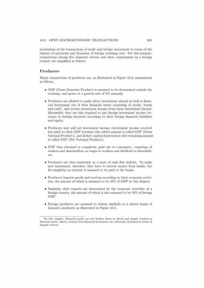
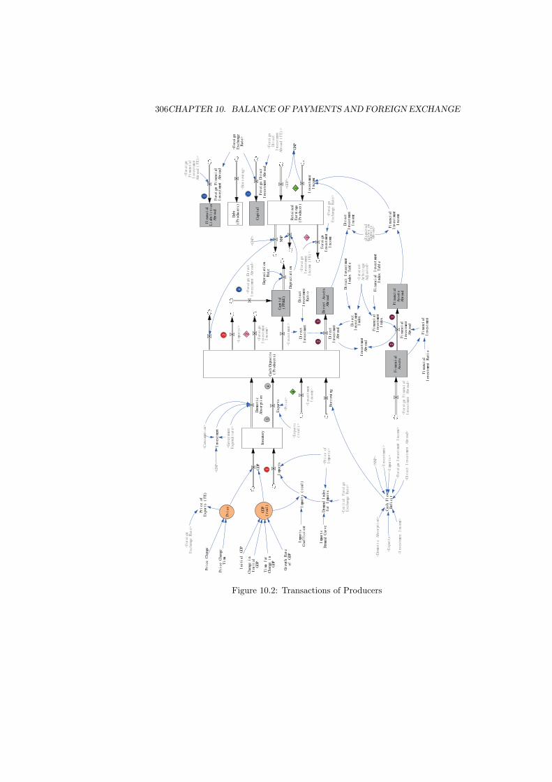
Major transactions of producers are, as illustrated in Figure 10.2, summarizedas follows.
• GDP (Gross Domestic Product) is assumed to be determined outside theeconomy, and grows at a growth rate of 2% annually.
• Producers are allowed to make direct investment abroad as well as finan-cial investment out of their financial assets consisting of stocks, bondsand cash2, and receive investment income from these investment abroad.Meanwhile, they are also required to pay foreign investment income (re-turns) to foreign investors according to their foreign financial liabilitiesand equity.
• Producers now add net investment income (investment income receivedless paid) to their GDP revenues (the added amount is called GNP (GrossNational Product)), and deduct capital depreciation (the remaining amountis called NNP (Net National Product)).
• NNP thus obtained is completely paid out to consumers, consisting ofworkers and shareholders, as wages to workers and dividend to sharehold-ers.
• Producers are thus constantly in a state of cash flow deficits. To makenew investment, therefore, they have to borrow money from banks, butfor simplicity no interest is assumed to be paid to the banks.
• Producers imports goods and services according to their economic activi-ties, the amount of which is assumed to be 10% of GDP in this chapter.
• Similarly, their exports are determined by the economic activities of aforeign country, the amount of which is also assumed to be 10% of foreignGDP.
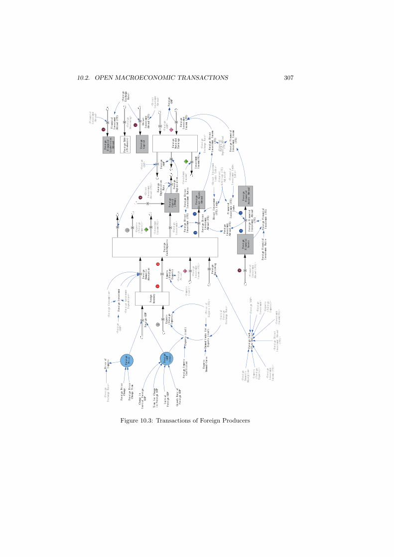
• Foreign producers are assumed to behave similarly as a mirror image ofdomestic producers as illustrated in Figure 10.3.
2In this chapter, financial assets are not broken down in detail and simply treated asfinancial assets. Hence, returns from financial investment are uniformly evaluated in terms ofdeposit returns.
306CHAPTER 10. BALANCE OF PAYMENTS AND FOREIGN EXCHANGE
Inve
ntory
Cas
h/D
epos
its
(P
rod
ucer
s)
1
2
Ex
por
ts
14
Di
rec
t A
sset
sA
broa
dD
ir
ect
Inv
estm
ent
Abr
oad
Di
rec
tI
nves
tmen
t
Fi
nanc
ial
Inv
estm
ent
Imp
orts
<For
eign
Ex
cha
nge
Rat
e>
Imp
orts
(
rea
l)
Pr
ice
ofE
xpo
rts
(
FE
)
<Pr
ice
ofI
mpor
ts>
Dem
and
Ind
exf
or
Imp
orts
Imp
orts
Dem
and
Cur
ve
<For
eign
Di
rec
tI
nves
tmen
tA
broa
d (
FE
)>
Pr
ice
Cha
nge
Pr
ice
Cha
nge
Ti
me
<Ex
por
ts(
rea
l)
>I
mpor
tsC
oef
fi
ci
ent
<Ini
tial
F
orei
gnE
xcha
nge
Rat
e>
Ret
aine
dE
arni
ngs
(P
rod
ucer
)
Inv
estm
ent
Inc
ome
For
eign
Inv
estm
ent
Inc
ome
<Inv
estm
ent
Inc
ome>
<For
eign
Inv
estm
ent
Inc
ome>
<Imp
orts
>
Fi
nanc
ial
Li
abi
li
ties
Abr
oad
12
For
eign
F
ina
nci
alI
nves
tmen
t A
broa
d
1
4
114
1
2
<Ex
pecte
dR
etur
n on
Dep
osi
tsA
broa
d>
GD
P(
rea
l)
Fi
nanc
ial
Asset
sA
broa
dF
ina
nci
alI
nves
tmen
tA
broa
d
<For
eign
Fi
nanc
ial
Inv
estm
ent
Abr
oad
(F
E)
>
Inv
estm
ent
Abr
oad
Fi
nanc
ial
Inv
estm
ent
Inc
ome
Ini
tial
G
DP
Gr
owth
R
ate
of
GD
P
<Int
eres
tA
rbi
trag
eA
djus
ted>
Cha
nge
in
Ini
tial
GD
P
Ti
me
for
Cha
nge
in
GD
P
Di
rec
tI
nves
tmen
tI
ndex
Di
rec
t I
nves
tmen
tI
ndex
T
abl
e
Fi
nanc
ial
Inv
estm
ent
Ind
ex
Fi
nanc
ial
I
nves
tmen
tI
ndex
T
abl
e
GD
P
<GD
P>
NN
P
<For
eign
Ex
cha
nge
Rat
e>
Inv
estm
ent
Dom
esti
cA
bsor
pti
on
<Inv
estm
ent>
Bor
row
ing
<Dom
esti
c
Abs
orpt
ion
>
<Ex
por
ts>
<NN
P>
<Imp
orts
>
<Inv
estm
ent>
Cas
h F
low
Def
ici
t
Cap
ita
l(
PP
&E
)
Deb
t(
Pr
oduc
ers)
<Bor
row
ing
>
<Gov
ernm
ent
Ex
pend
itu
re>
Pr
ice
<Pr
ice>
Fi
nanc
ial
Asset
s<I
nves
tmen
t I
ncom
e><F
orei
gn
Inv
estm
ent
Inc
ome>
<Di
rec
t I
nves
tmen
t A
broa
d>
Di
rec
tI
nves
tmen
tI
ncom
e
21
<For
eign
Inv
estm
ent
Inc
ome
(F
E)
>
Cap
ita
lF
orei
gn
Di
rec
tI
nves
tmen
t A
broa
d
<For
eign
Ex
cha
nge
Rat
e>
<For
eign
D
ir
ect
Inv
estm
ent
Abr
oad>
1
<For
eign
F
ina
nci
alI
nves
tmen
t A
broa
d>
Dep
rec
iat
ion
Dep
rec
iat
ion
Rat
e
Di
rec
tI
nves
tmen
tR
ati
o
Fi
nanc
ial
Inv
estm
ent
Rat
io
<Con
sum
pti
on>
GN
P
<GN
P>
<GN
P>
Figure 10.2: Transactions of Producers
10.2. OPEN MACROECONOMIC TRANSACTIONS 307
Fore
ign
Inve
ntory
For
eign
Cas
h/D
epos
its
14
1
2
For
eign
Di
rec
t A
sset
sA
broa
d
Ex
por
ts
(r
eal
)
For
eign
Pr
ice
For
eign
D
ir
ect
Inv
estm
ent
Abr
oad
(F
E)
Ex
por
ts(
For
eign
Imp
orts
)
Imp
orts
(F
orei
gnE
xpo
rts
)
<Pr
ice
ofE
xpo
rts
(
FE
)>
Dem
and
Ind
ex
for
Ex
por
ts
(r
eal
)
Ex
por
tsD
eman
d C
urv
e
Pr
ice
ofI
mpor
ts
<For
eign
Ex
cha
nge
Rat
e>
For
eign
D
ir
ect
Inv
estm
ent
(F
E)
For
eign
F
ina
nci
alI
nves
tmen
t (
FE
)
For
eign
I
mpor
tsC
oef
fi
ci
ent
<Di
rec
tI
nves
tmen
tA
broa
d>
<Imp
orts
(r
eal
)>
For
eign
Ret
aine
dE
arni
ngs
For
eign
Inv
estm
ent
Inc
ome
(F
E)
Inv
estm
ent
Inc
ome(
FE
)
<Inv
estm
ent
Inc
ome(
FE
)>
<For
eign
Inv
estm
ent
Inc
ome
(F
E)
>
<Ex
por
ts(
For
eign
Imp
orts
)>
<Ini
tial
For
eign
Ex
cha
nge
Rat
e>
For
eign
Fi
nanc
ial
Li
abi
li
ties
Abr
oad
Fi
nanc
ial
Inv
estm
ent
Abr
oad
(F
E)
1
4
12
1
2
1
4
<Ex
pecte
dR
etur
n on
Dep
osi
ts
Abr
oad
(F
E)
>
For
eign
GD
P(
rea
l)
<Fi
nanc
ial
Inv
estm
ent
Abr
oad>
For
eign
Fi
nanc
ial
Asset
s
Abr
oad
For
eign
F
ina
nci
alI
nves
tmen
t A
broa
d(
FE
)
For
eign
Inv
estm
ent
Abr
oad
(F
E)
For
eign
F
ina
nci
alI
nves
tmen
t I
ncom
e(
FE
)
Ini
tial
For
eign
G
DP
Gr
owth
R
ate
ofF
orei
gn
GD
P
<Int
eres
tA
rbi
trag
e (
FE
)A
djus
ted>
Cha
nge
in
Ini
tial
F
orei
gnG
DP
Ti
me
for
C
hang
ei
n F
orei
gn
GD
P
Di
rec
t I
nves
tmen
t(
FE
)
Ind
ex
<Di
rec
t I
nves
tmen
tI
ndex
T
abl
e>
Fi
nanc
ial
Inv
estm
ent
(F
E)
Ind
ex
<Fi
nanc
ial
Inv
estm
ent
Ind
exT
abl
e>
<For
eign
Pr
ice>
For
eign
G
DP
For
eign
Dom
esti
cA
bsor
pti
on
For
eign
I
nves
tmen
t
<For
eign
Ex
cha
nge
Rat
e>
<For
eign
GD
P>
For
eign
NN
P
For
eign
Cap
ita
l(
PP
&E
)
<For
eign
G
over
nmen
tE
xpe
ndi
tur
e>
<For
eign
Inv
estm
ent>
For
eign
C
ash
Fl
ow
Def
ici
t
<For
eign
Dom
esti
cA
bsor
pti
on>
<Imp
orts
(F
orei
gnE
xpo
rts
)>
<For
eign
N
NP
>
<For
eign
Inv
estm
ent>
<Ex
por
ts(
For
eign
Imp
orts
)>
For
eign
Bor
row
ing
For
eign
D
ebt
(P
rod
ucer
s)
<For
eign
Bor
row
ing
>
For
eign
Fi
nanc
ial
Asset
s
<For
eign
Inv
estm
ent
Inc
ome
(F
E)
>
<Inv
estm
ent
Inc
ome(
FE
)>
<For
eign
D
ir
ect
Inv
estm
ent
Abr
oad
(F
E)
>
For
eign
D
ir
ect
Inv
estm
ent
Inc
ome
(F
E)
<Inv
estm
ent
Inc
ome>
For
eign
Cap
ita
lD
ir
ect
Inv
estm
ent
Abr
oad
(F
E)
<Di
rec
tI
nves
tmen
tA
broa
d (
FE
)>
<For
eign
Ex
cha
nge
Rat
e>
<Fi
nanc
ial
Inv
estm
ent
Abr
oad
(F
E)
>
1
41
2
For
eign
Dep
rec
iat
ion
For
eign
Dep
rec
iat
ion
Rat
e
For
eign
D
ir
ect
Inv
estm
ent
Rat
io
For
eign
F
ina
nci
alI
nves
tmen
t R
ati
o
<For
eign
C
onsum
pti
on>
For
eign
GN
P
<For
eign
GN
P>
<For
eign
GN
P>
For
eign
P
ri
ce
Cha
nge
For
eign
P
ri
ce
Cha
nge
Ti
me
Figure 10.3: Transactions of Foreign Producers
308CHAPTER 10. BALANCE OF PAYMENTS AND FOREIGN EXCHANGE
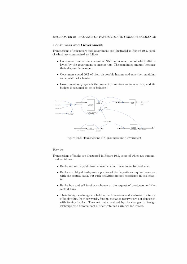
Consumers and GovernmentTransactions of consumers and government are illustrated in Figure 10.4, someof which are summarized as follows.
• Consumers receive the amount of NNP as income, out of which 20% islevied by the government as income tax. The remaining amount becomestheir disposable income.
• Consumers spend 60% of their disposable income and save the remainingas deposits with banks.
• Government only spends the amount it receives as income tax, and itsbudget is assumed to be in balance.
Deposi t s( Consumer s)
ConsumerEqui t y
I ni t i al Deposi t s( Consumer s)
Ret ai nedEar ni ngs
( Gover nment )Cash
( Gover nment )
I ncome Tax
Tax Revenues
I ncome Tax Rat e
<Tax Revenues>
Savi ng
<I ncome Tax>
Gover nmentExpendi t ur e
<NNP><NNP>
Consumpt i on
<Consumpt i on>
Net For ei gnI nvest ment
<I nvest ment >
<Depr eci at i on>
Figure 10.4: Transactions of Consumers and Government
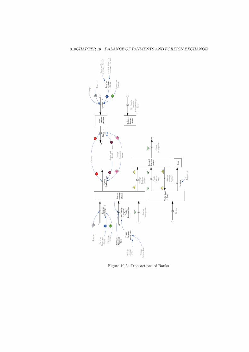
BanksTransactions of banks are illustrated in Figure 10.5, some of which are summa-rized as follows.
• Banks receive deposits from consumers and make loans to producers.
• Banks are obliged to deposit a portion of the deposits as required reserveswith the central bank, but such activities are not considered in this chap-ter.
• Banks buy and sell foreign exchange at the request of producers and thecentral bank.
• Their foreign exchange are held as bank reserves and evaluated in termsof book value. In other words, foreign exchange reserves are not depositedwith foreign banks. Thus net gains realized by the changes in foreignexchange rate become part of their retained earnings (or losses).
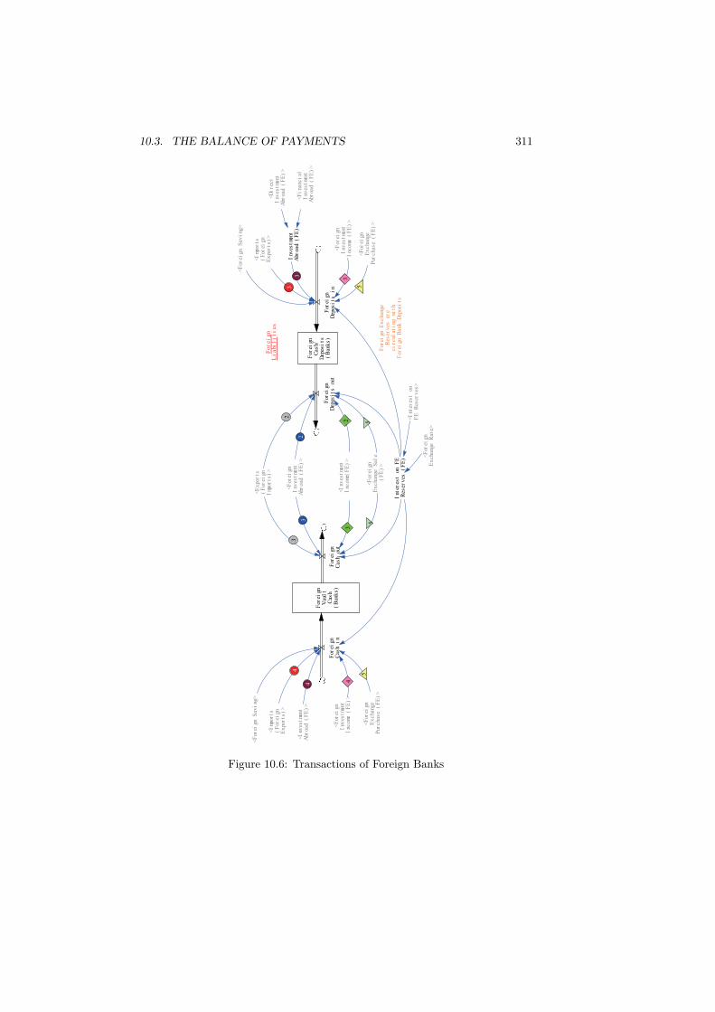
10.3. THE BALANCE OF PAYMENTS 309
• Foreign currency is assumed to play a role of key currency or vehiclecurrency. Accordingly foreign banks need not set up foreign exchangeaccount. This is a point where a mirror image of open macroeconomicsymmetry breaks down, as illustrated in Figure 10.6.
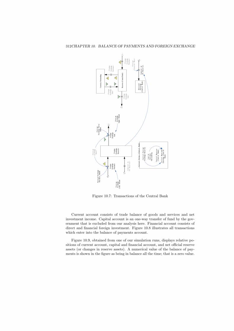
Central BankIn the integrated model of the previous chapter, the central bank played animportant role of providing a means of transactions and store of value; thatis, currency, and its sources of assets against which currency is issued wereassumed to be gold, loan and government securities. Transactions of the centralbank here are exceptionally simplified, as illustrated in Figure 10.7, so long asnecessary for the analytical purpose in this chapter.
• The central bank can control the amount of money supply through mon-etary policies such as the manipulation of required reserve ratio and openmarket operations. However, such a role of money supply by the centralbank is not considered here.
• The central bank is allowed to intervene foreign exchange market; thatis, it can buy and sell foreign exchange to keep a foreign exchange ratiostable. These transactions are manipulated with commercial banks, whichinescapably change the amount of currency outstanding and, hence, moneysupply. In this chapter, however, such an effect of money supply on interestrate is assumed to be out of consideration.
• Foreign exchange reserves held by the central bank is assumed to be de-posited with foreign banks so that it receives interest payments.
• The central bank of foreign country is excluded simply because foreigncurrency is assumed to be a vehicle currency, and it needs not to holdforeign reserves (that is, its own currency) to stabilize its own exchangerate in this simplified open macroeconomy.
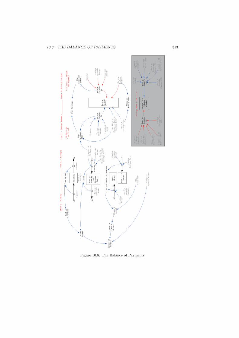
10.3 The Balance of PaymentsAll transactions with a foreign country such as foreign trade and foreign invest-ment (that is, payments and receipts of foreign exchange) are booked accordingto a double entry bookkeeping rule, and such a bookkeeping record is called thebalance of payments. According to [44] in page 295, all payments are recordedin the debit side with a minus sign, while all receipts are recorded in the creditside with plus sign. Hence, by definition, the balance of payments are keptin balance all the time. It consists of current account, capital and financialaccount, and net official reserve assets.
310CHAPTER 10. BALANCE OF PAYMENTS AND FOREIGN EXCHANGE
2
Req
uire
dR
eser
ves
(Ban
ks)
3
<F
ore
ign
Exc
hang
e S
ale>
2
<F
ore
ign
Exc
hang
eS
ale>
3
2
<F
ore
ign
Exc
hang
eP
urch
ase>
3
Fo
reig
nE
xcha
nge
(Ban
ks)
<E
xpo
rts>
<Im
po
rts>
3
11
<F
ore
ign
Exc
hang
eP
urch
ase>
<F
ore
ign
Exc
hang
e S
ale>
Fore
ign
Exc
hang
e(B
ook V
alue
)
<F
ore
ign
Exc
hang
e(F
E)>
Ret
aine
dE
arni
ngs
(Ban
ks)
Net
Gai
ns b
yC
hang
es in
Fo
reig
nE
xcha
nge
Rat
e
<N
et G
ains
by
Cha
nges
inF
ore
ign
Exc
hang
eR
ate>
Net
Gai
nsA
dju
stm
ent
Tim
e
<F
ore
ign
Inve
stm
ent
Inco
me>
<F
ore
ign
Exc
hang
e R
ate>
Cas
h/D
epos
its
(B
ank
s)
<Ex
por
ts>
Dep
osi
ts
in
Dep
osi
tsou
t
4
Vau
lt
Cas
h(
Ban
ks)
23
3<F
orei
gn
Fi
nanc
ial
Inv
estm
ent
Abr
oad>
4
34
23
4
4
For
eign
Ex
cha
nge
out
<Inv
estm
ent
Abr
oad>
For
eign
Ex
cha
nge
in
<Sav
ing
>
<Sav
ing
>
Len
ding
<Bor
row
ing
>
Loa
n
<Inv
estm
ent
Inc
ome>
<Inv
estm
ent
Inc
ome>
For
eign
Inv
estm
ent
Abr
oad
<For
eign
D
ir
ect
Inv
estm
ent
Abr
oad>
<For
eign
Inv
estm
ent
Abr
oad>
Figure 10.5: Transactions of Banks
10.3. THE BALANCE OF PAYMENTS 311
4
2
For
eign
Vau
lt
Cas
h(
Ban
ks)
For
eign
Cas
h/D
epos
its
(B
ank
s)
For
eign
Dep
osi
ts
in
For
eign
Dep
osi
ts
out
<Imp
orts
(F
orei
gnE
xpo
rts
)>
For
eign
Cas
h i
n
4
<Imp
orts
(F
orei
gnE
xpo
rts
)>
For
eign
Cas
h ou
t
Fo
re
ig
nL
ia
bi
li
ti
es
<Ex
por
ts(
For
eign
Imp
orts
)>
<Inv
estm
ent
Inc
ome(
FE
)>
33
3<F
ina
nci
alI
nves
tmen
tA
broa
d (
FE
)>
42
3
23
3
<For
eign
Inv
estm
ent
Abr
oad
(F
E)
>
<For
eign
Ex
cha
nge
Pur
cha
se
(F
E)
><F
orei
gnE
xcha
nge
Pur
cha
se
(F
E)
>
<For
eign
Ex
cha
nge
Sal
e(
FE
)>
Int
eres
t on
F
ER
eser
ves
(
FE
)
<Int
eres
t on
FE
R
eser
ves
>
<For
eign
Ex
cha
nge
Rat
e>
55
55
<For
eign
S
avi
ng>
<For
eign
S
avi
ng>
<For
eign
Inv
estm
ent
Inc
ome
(F
E)
>
<For
eign
Inv
estm
ent
Inc
ome
(F
E)
>
Inv
estm
ent
Abr
oad
(F
E)
<Di
rec
tI
nves
tmen
tA
broa
d (
FE
)>
<Inv
estm
ent
Abr
oad
(F
E)
>
For
eign
E
xcha
nge
Res
erv
es
are
ci
rcul
ati
ng
wi
thF
orei
gn
Ban
k
Dep
osi
ts
Figure 10.6: Transactions of Foreign Banks
312CHAPTER 10. BALANCE OF PAYMENTS AND FOREIGN EXCHANGE
Ini
tial
V
alue
s
(C
entr
al
Ban
k)
Fore
ign
Exc
hang
eR
eser
ves
Cur
renc
y O
utst
and
ing
Res
erve
s (C
entr
al B
ank)
Fore
ign
Exc
hang
eS
ale
1
<F
ore
ign
Exc
hang
eS
ale>2
<F
ore
ign
Exc
hang
eS
ale>
3
Fore
ign
Exc
hang
eP
urch
ase1
<F
ore
ign
Exc
hang
eP
urch
ase>
2
<F
ore
ign
Exc
hang
eP
urch
ase>
3
<For
eign
Ex
cha
nge
Rat
e>
For
eign
Ex
cha
nge
Low
er
Bou
nd
For
eign
Ex
cha
nge
Upp
er
Bou
nd
For
eign
E
xcha
nge
Pur
cha
se
Amo
unt
For
eign
Ex
cha
nge
Sal
esA
moun
t
4
4
Ret
aine
dE
arni
ngs
(C
entr
al
Ban
k)
Int
eres
t on
FE
R
eser
ves<F
orei
gnI
nter
est
Rat
e>
<Int
eres
t on
FE
R
eser
ves
>
Ini
tial
F
orei
gnE
xcha
nge
Res
erv
es
Ini
tial
Cur
ren
cy
Out
sta
ndi
ng
Ini
tial
R
eser
ves
(C
entr
al
Ban
k)
Ini
tial
R
eati
ned
Ear
ning
s
(C
entr
alB
ank
)
Figure 10.7: Transactions of the Central Bank
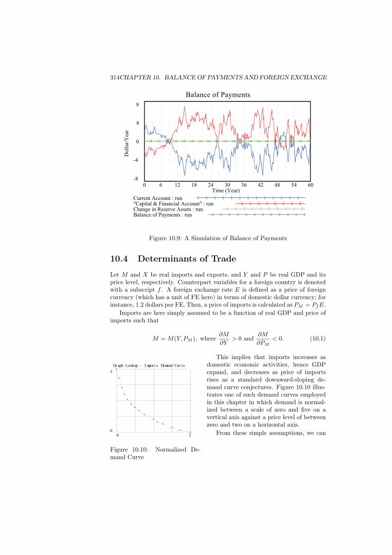
Current account consists of trade balance of goods and services and netinvestment income. Capital account is an one-way transfer of fund by the gov-ernment that is excluded from our analysis here. Financial account consists ofdirect and financial foreign investment. Figure 10.8 illustrates all transactionswhich enter into the balance of payments account.
Figure 10.9, obtained from one of our simulation runs, displays relative po-sitions of current account, capital and financial account, and net official reserveassets (or changes in reserve assets). A numerical value of the balance of pay-ments is shown in the figure as being in balance all the time; that is a zero value.
10.3. THE BALANCE OF PAYMENTS 313
Inv
ento
ry
<Imp
orts
><E
xpo
rts
>
De
bi
t
(-
P
ay
me
nt
)_
__
__
__
__
__
__
__
__
__
__
__
_
Cr
edi
t
(+
R
ec
ei
pt
)
For
eign
Ex
cha
nge
(B
ank
s)
<Ex
por
ts>
<For
eign
Ex
cha
nge
Pur
cha
se>
<For
eign
Ex
cha
nge
Sal
e>
<For
eign
Inv
estm
ent
Inc
ome>
<Net
G
ains
by
Cha
nges
i
n F
orei
gnE
xcha
nge
Rat
e>
<Imp
orts
>
Oth
erI
nves
tmen
t(
Deb
it)
Oth
erI
nves
tmen
t(
Cr
edi
t)
Goo
ds
&S
erv
ices
Inc
ome
Di
rec
t an
d P
ortf
oli
o I
nves
tmen
t
Cha
nge
in
Res
erv
e A
sset
s
Tr
ade
Bal
ance
Fi
nanc
ial
Accou
nt
Cur
ren
tA
ccou
nt
Cap
ita
l
&F
ina
nci
alA
ccou
nt
Oth
er
Inv
estm
ent
Bal
ance
ofP
ayme
nts
<Oth
erI
nves
tmen
t>
For
eign
Ex
cha
nge
out
<Inv
estm
ent
Abr
oad>
For
eign
Ex
cha
nge
in
De
bi
t
(-
F
or
ei
gn
P
ay
me
nt
)_
__
__
__
__
__
__
_
Cr
edi
t
(+
F
or
ei
gn
R
ec
ei
pt
)
Ret
aine
dE
arni
ngs
and
Con
sum
erE
qui
ty
Ear
ning
s
in
<For
eign
Inv
estm
ent
Inc
ome>
<Net
G
ains
by
Cha
nges
i
n F
orei
gnE
xcha
nge
Rat
e>
Asset
sA
broa
d
<Inv
estm
ent
Abr
oad>
For
eign
C
ash/
Dep
osi
ts(
Ban
ks)
For
eign
Dep
osi
tsou
t
<Ex
por
ts(
For
eign
Imp
orts
)>
<For
eign
Ex
cha
nge
Sal
e(
FE
)>
<For
eign
Inv
estm
ent
Abr
oad
(F
E)
>
<Inv
estm
ent
Inc
ome(
FE
)>
For
eign
Dep
osi
tsi
n
<For
eign
Ex
cha
nge
Pur
cha
se
(F
E)
>
<Imp
orts
(F
orei
gnE
xpo
rts
)>
<For
eign
Ex
cha
nge
Pur
cha
se>
<For
eign
Ex
cha
nge
Sal
e>
<Cha
nge
in
Res
erv
e A
sset
s>
(F
or
ei
gn
B
an
k
Li
abi
li
ti
es
)(F
E
De
po
si
ts
A
br
oa
df
or
P
ay
me
nt
)
<Int
eres
t on
F
ER
eser
ves
(
FE
)>
<Int
eres
t on
FE
R
eser
ves
>
(F
E
Re
ce
ipt
sf
ro
m
Abr
oa
d)
Li
abi
li
ties
Abr
oad
<Ini
tial
Inv
ento
ry
>
<Int
eres
t on
F
ER
eser
ves
(
FE
)>
<For
eign
Sav
ing
>
<Inv
estm
ent
Inc
ome>
<For
eign
Inv
estm
ent
Inc
ome
(F
E)
>
<For
eign
Inv
estm
ent
Abr
oad>
<Inv
estm
ent
Abr
oad
(F
E)
>
<For
eign
Inv
estm
ent
Abr
oad>
<Inv
estm
ent
Inc
ome>
Figure 10.8: The Balance of Payments
314CHAPTER 10. BALANCE OF PAYMENTS AND FOREIGN EXCHANGE
Balance of Payments
8
4
0
-4
-8
4 4 4 4 4 4 4 4 4 4 4 4 4 4 4 4 4 4 4 43 3 3 3 3 3 3 3 3 3 3 3 3 3 3 3 3 3 3 3
2 22
2
22
22
2
2
2
22
22
2
2
2
2
2
11
1
1
11 1
1
1 1
1
11
1
1
11
11
1
0 6 12 18 24 30 36 42 48 54 60Time (Year)
Do
llar
/Yea
r
Current Account : run 1 1 1 1 1 1 1 1 1 1 1 1 1
"Capital & Financial Account" : run 2 2 2 2 2 2 2 2
Change in Reserve Assets : run 3 3 3 3 3 3 3 3 3 3
Balance of Payments : run 4 4 4 4 4 4 4 4 4 4 4 4
Figure 10.9: A Simulation of Balance of Payments
10.4 Determinants of Trade
Let M and X be real imports and exports, and Y and P be real GDP and itsprice level, respectively. Counterpart variables for a foreign country is denotedwith a subscript f . A foreign exchange rate E is defined as a price of foreigncurrency (which has a unit of FE here) in terms of domestic dollar currency; forinstance, 1.2 dollars per FE. Then, a price of imports is calculated as PM = PfE.
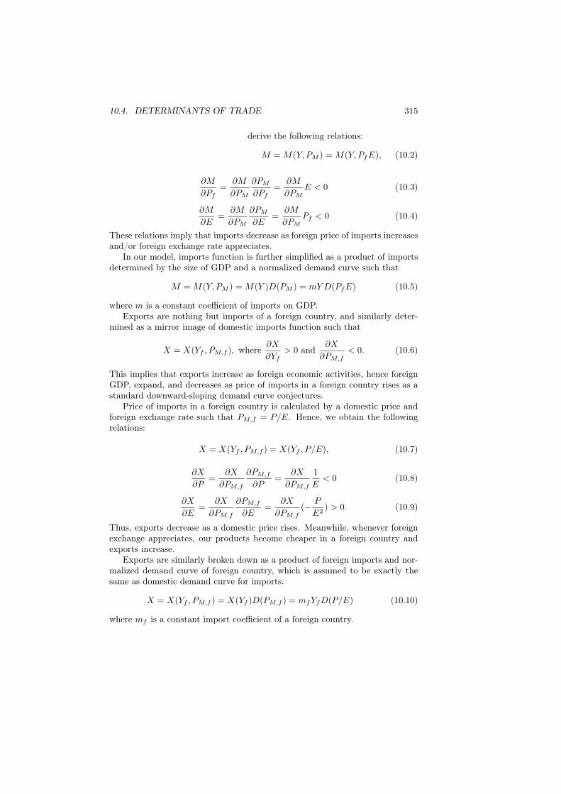
Imports are here simply assumed to be a function of real GDP and price ofimports such that
M = M(Y, PM ), where∂M
∂Y> 0 and
∂M
∂PM< 0. (10.1)
Gr aph Lookup - I mpor t s Demand Curve
5
00 2
Figure 10.10: Normalized De-mand Curve
This implies that imports increases asdomestic economic activities, hence GDPexpand, and decreases as price of importsrises as a standard downward-sloping de-mand curve conjectures. Figure 10.10 illus-trates one of such demand curves employedin this chapter in which demand is normal-ized between a scale of zero and five on avertical axis against a price level of betweenzero and two on a horizontal axis.
From these simple assumptions, we can
10.4. DETERMINANTS OF TRADE 315
derive the following relations:
M = M(Y, PM ) = M(Y, PfE), (10.2)
∂M
∂Pf=
∂M
∂PM
∂PM
∂Pf=
∂M
∂PME < 0 (10.3)
∂M
∂E=
∂M
∂PM
∂PM
∂E=
∂M
∂PMPf < 0 (10.4)
These relations imply that imports decrease as foreign price of imports increasesand/or foreign exchange rate appreciates.
In our model, imports function is further simplified as a product of importsdetermined by the size of GDP and a normalized demand curve such that
M = M(Y, PM ) = M(Y )D(PM ) = mYD(PfE) (10.5)
where m is a constant coefficient of imports on GDP.Exports are nothing but imports of a foreign country, and similarly deter-
mined as a mirror image of domestic imports function such that
X = X(Yf , PM,f ), where∂X
∂Yf> 0 and
∂X
∂PM,f< 0. (10.6)
This implies that exports increase as foreign economic activities, hence foreignGDP, expand, and decreases as price of imports in a foreign country rises as astandard downward-sloping demand curve conjectures.
Price of imports in a foreign country is calculated by a domestic price andforeign exchange rate such that PM,f = P/E. Hence, we obtain the followingrelations:
X = X(Yf , PM,f ) = X(Yf , P/E), (10.7)
∂X
∂P=
∂X
∂PM,f
∂PM,f
∂P=
∂X
∂PM,f
1
E< 0 (10.8)
∂X
∂E=
∂X
∂PM,f
∂PM,f
∂E=
∂X
∂PM,f(− P
E2) > 0. (10.9)
Thus, exports decrease as a domestic price rises. Meanwhile, whenever foreignexchange appreciates, our products become cheaper in a foreign country andexports increase.
Exports are similarly broken down as a product of foreign imports and nor-malized demand curve of foreign country, which is assumed to be exactly thesame as domestic demand curve for imports.
X = X(Yf , PM,f ) = X(Yf )D(PM,f ) = mfYfD(P/E) (10.10)
where mf is a constant import coefficient of a foreign country.
316CHAPTER 10. BALANCE OF PAYMENTS AND FOREIGN EXCHANGE
Let us define trade balance as
TB(E;Y, Yf , P, Pf ) = X(E;Yf , P )−M(E;Y, Pf ) (10.11)
Then we have∂TB
∂Y= −∂M
∂Y< 0,
∂TB
∂Yf=
∂X
∂Yf> 0, (10.12)
∂TB
∂P=
∂X
∂P< 0,
∂TB
∂Pf= − ∂M
∂Pf> 0. (10.13)
∂TB
∂E=
∂X
∂E− ∂M
∂E> 0. (10.14)
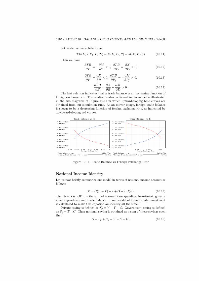
The last relation indicates that a trade balance is an increasing function offoreign exchange rate. The relation is also confirmed in our model as illustratedin the two diagrams of Figure 10.11 in which upward-sloping blue curves areobtained from our simulation runs. As an mirror image, foreign trade balanceis shown to be a decreasing function of foreign exchange rate, as indicated bydownward-sloping red curves.
Tr ade Bal ance vs E
8 Dol l ar / Year8 FE/ Year
4 Dol l ar / Year4 FE/ Year
0 Dol l ar / Year0 FE/ Year
- 4 Dol l ar / Year- 4 FE/ Year
- 8 Dol l ar / Year- 8 FE/ Year
0. 940 0. 950 0. 960 0. 970 0. 980 0. 990 1For ei gn Exchange Rat e
Tr ade Bal ance : r un Dol l ar / Year" For ei gn Tr ade Bal ance ( FE) " : r un FE/ Year
Tr ade Bal ance vs E
8 Dol l ar / Year8 FE/ Year
4 Dol l ar / Year4 FE/ Year
0 Dol l ar / Year0 FE/ Year
- 4 Dol l ar / Year- 4 FE/ Year
- 8 Dol l ar / Year- 8 FE/ Year
1 1. 020 1. 040 1. 060For ei gn Exchange Rat e
Tr ade Bal ance : r un Dol l ar / Year" For ei gn Tr ade Bal ance ( FE) " : r un FE/ Year
Figure 10.11: Trade Balance vs Foreign Exchange Rate
National Income IdentityLet us now briefly summarize our model in terms of national income account asfollows:
Y = C(Y − T ) + I +G+ TB(E) (10.15)That is to say, GDP is the sum of consumption spending, investment, govern-ment expenditure and trade balance. In our model of foreign trade, investmentis calculated to make this equation an identity all the time.
Private saving is defined as Sp = Y − T − C. Government saving is definedas Sg = T −G. Then national saving is obtained as a sum of these savings suchthat
S = Sp + Sg = Y − C −G, (10.16)
10.5. DETERMINANTS OF FOREIGN INVESTMENT 317
which reduces toS − I = TB(E). (10.17)
Saving less investment is called net foreign investment, which is equal to tradebalance. This becomes another way of describing the above national incomeidentity in terms of net foreign investment and trade balance.
10.5 Determinants of Foreign InvestmentForeign investment consists of direct investment and financial investment suchas stocks, bonds and cash, which constitute financial assets. In this chapterfinancial assets are not specified without losing generality as already mentionedin the footnote above. Foreign investments are here assumed to be determinedon a principle of foreign exchange market efficiency under the uncovered interestrate parity (UIP) condition as explained in standard textbooks such as [44] and[57].
Let i and R be interest rate and a rate of return from financial investment,and Ee be an expected foreign exchange rate. A rate of return from a bankdeposit is the same as the interest rate:
R = i (10.18)
An expected return from a deposit with a foreign bank is calculated as
Rf = (1 + if )Ee
E− 1 (10.19)
Thus we obtain∂Rf
∂E= − (1 + if )Ee
E2< 0 (10.20)
∂Rf
∂Ee=
(1 + if )
E> 0 (10.21)
This implies that a rate of return from foreign financial investment decreases ifforeign exchange rate appreciates, but it increases when foreign exchange rateis expected to appreciate.
Let us define an expected return arbitrage as
A(E,Ee; i, if ) = Rf (E,Ee; if )−R(i) (10.22)
and net capital flow(NCF ) as
NCF = Foreign Investment Abroad − Investment Abroad (10.23)
This is the amount of capital we receive from foreign country’s investment lessthe amount we invest abroad. Under the assumption of an efficient financialmarket, if expected returns are greater in a foreign country and an expectedreturn arbitrage becomes positive, then financial capital continues to outflow
318CHAPTER 10. BALANCE OF PAYMENTS AND FOREIGN EXCHANGE
until the arbitrage ceases to exist. In a similar fashion, if expected returns aregreater in a domestic market and an expected return arbitrage becomes negative,then financial capital continues to inflow until the arbitrage disappears. Hence,so long as a foreign exchange market is efficient, the relation between net capitalflow and an expected return arbitrage become as follows:
!NCF < 0 if A > 0NCF > 0 if A < 0
(10.24)
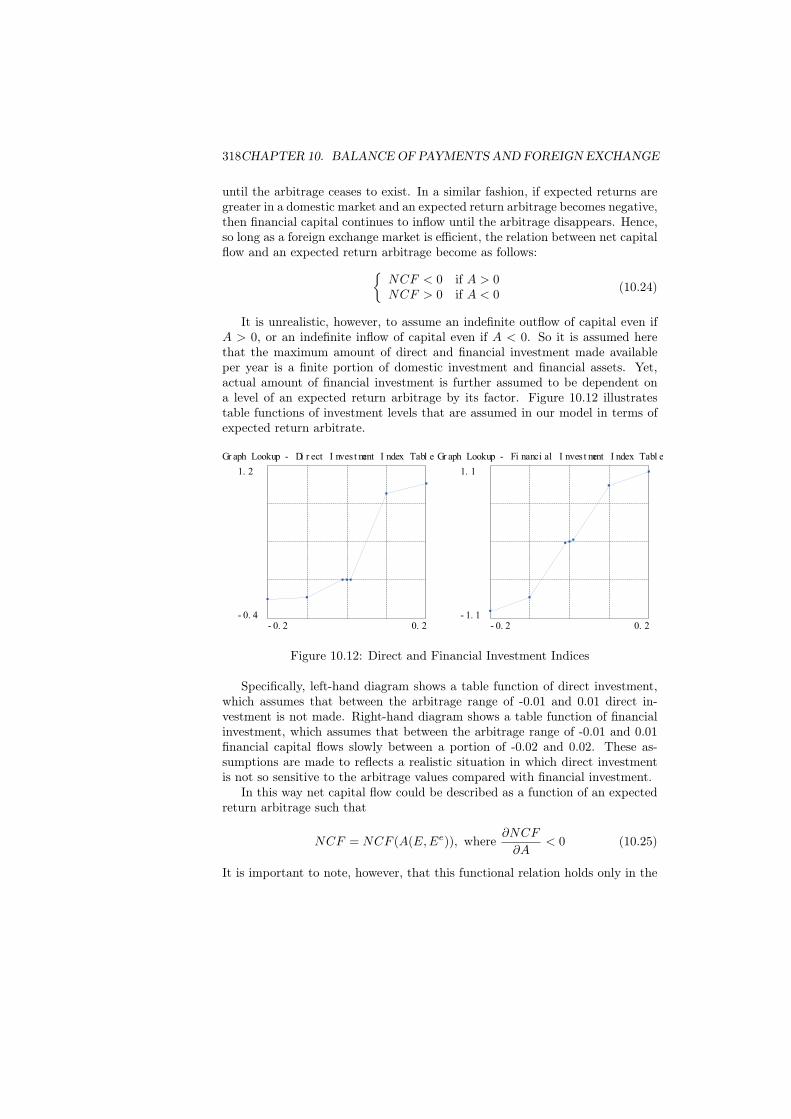
It is unrealistic, however, to assume an indefinite outflow of capital even ifA > 0, or an indefinite inflow of capital even if A < 0. So it is assumed herethat the maximum amount of direct and financial investment made availableper year is a finite portion of domestic investment and financial assets. Yet,actual amount of financial investment is further assumed to be dependent ona level of an expected return arbitrage by its factor. Figure 10.12 illustratestable functions of investment levels that are assumed in our model in terms ofexpected return arbitrate.
Gr aph Lookup - Di r ect I nvest ment I ndex Tabl e
1. 2
- 0. 4- 0. 2 0. 2
Gr aph Lookup - Fi nanci al I nvest ment I ndex Tabl e
1. 1
- 1. 1- 0. 2 0. 2
Figure 10.12: Direct and Financial Investment Indices
Specifically, left-hand diagram shows a table function of direct investment,which assumes that between the arbitrage range of -0.01 and 0.01 direct in-vestment is not made. Right-hand diagram shows a table function of financialinvestment, which assumes that between the arbitrage range of -0.01 and 0.01financial capital flows slowly between a portion of -0.02 and 0.02. These as-sumptions are made to reflects a realistic situation in which direct investmentis not so sensitive to the arbitrage values compared with financial investment.
In this way net capital flow could be described as a function of an expectedreturn arbitrage such that
NCF = NCF (A(E,Ee)), where∂NCF
∂A< 0 (10.25)
It is important to note, however, that this functional relation holds only in the
10.6. DYNAMICS OF FOREIGN EXCHANGE RATES 319
neighborhood of equilibrium, so do the following relations as well.
∂NCF
∂E=
∂NCF
∂A
∂A
∂E=
∂NCF
∂A
∂Rf
∂E> 0 (10.26)
∂NCF
∂Ee=
∂NCF
∂A
∂A
∂Ee=
∂NCF
∂A
∂Rf
∂Ee< 0 (10.27)
Whenever a foreign exchange rate begins to appreciate, an expected returnarbitrage declines, and capital begins to inflow, causing a positive net capitalflow. When foreign exchange rate is expected to appreciate, an expected returnarbitrage increases and capital begins to outflow, causing a negative net capitalflow. In this way, changes in a foreign exchange rate and its expectations playa crucial role for financial investment.
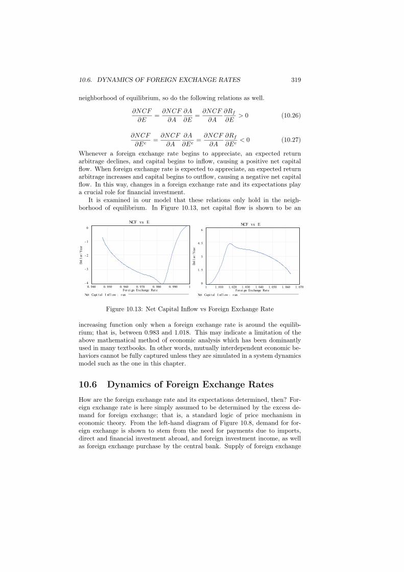
It is examined in our model that these relations only hold in the neigh-borhood of equilibrium. In Figure 10.13, net capital flow is shown to be an
NCF vs E
0
- 1
- 2
- 3
- 40. 940 0. 950 0. 960 0. 970 0. 980 0. 990 1
For ei gn Exchange Rat e
Dol
lar
/Yea
r
Net Capi t al I nf l ow : r un
NCF vs E
6
4. 5
3
1. 5
01 1. 010 1. 020 1. 030 1. 040 1. 050 1. 060 1. 070
For ei gn Exchange Rat e
Dol
lar
/Yea
r
Net Capi t al I nf l ow : r un
Figure 10.13: Net Capital Inflow vs Foreign Exchange Rate
increasing function only when a foreign exchange rate is around the equilib-rium; that is, between 0.983 and 1.018. This may indicate a limitation of theabove mathematical method of economic analysis which has been dominantlyused in many textbooks. In other words, mutually interdependent economic be-haviors cannot be fully captured unless they are simulated in a system dynamicsmodel such as the one in this chapter.
10.6 Dynamics of Foreign Exchange RatesHow are the foreign exchange rate and its expectations determined, then? For-eign exchange rate is here simply assumed to be determined by the excess de-mand for foreign exchange; that is, a standard logic of price mechanism ineconomic theory. From the left-hand diagram of Figure 10.8, demand for for-eign exchange is shown to stem from the need for payments due to imports,direct and financial investment abroad, and foreign investment income, as wellas foreign exchange purchase by the central bank. Supply of foreign exchange
320CHAPTER 10. BALANCE OF PAYMENTS AND FOREIGN EXCHANGE
results from the receipts from foreign country due to exports, foreign direct andfinancial investment abroad, and investment income from abroad, as well asforeign exchange sale by the central bank.
Hence, excess demand for foreign exchange is calculated as follows:
Excess Demand for Foreign Exchange= Imports - Exports
+ Investment Abroad - Foreign Investment Abroad+ Foreign Investment Income - Investment Income+ Foreign Exchange Purchase - Foreign Exchange Sale
= − Trade Balance (TB)
− Net Capital Flow (NCF )
− Net Investment Income (NII)
+ Net Exchange Reserves (NER)
(10.28)
Net investment income is derived from the financial assets invested abroadand here assumed to be dependent only on domestic and foreign interest rates.Net exchange reserves depend on the official foreign exchange intervention.Therefore, NII and NER are not dependent on foreign exchange rate and itsexpectations.
With these relations taken into consideration, dynamics of foreign exchangerate is mathematically expressed as a function of excess demand for foreignexchange, which in turn becomes a function of E and Ee as follows:
dE
dt= Ψ(−TB(E)−NCF (E,Ee)−NII +NER) = Ψ(E,Ee) (10.29)
On the other hand, a formation of expected foreign exchange rates is difficultto formalize. Here it is simply assumed that actual expectations of foreignexchange rate fluctuates randomly around the current exchange rate by thefactor of random normal distribution of Nrandom(m, sd) where (m, sd) denotesmean and standard deviation, and accordingly an expected foreign exchangerate is obtained as an adaptive expectation against the actual expectation ofrandom normal distribution.
Mathematically, dynamics of the expected foreign exchange rate thus definedis described as
dEe
dt= Φ(Nrandom(m, sd)E − Ee) = Φ(E,Ee) (10.30)
Thus, expected foreign exchange rate can be easily adjusted to the actual trendsand volatilities of various economic situations by refining values in mean andstandard deviation. Figure 10.14 illustrates how foreign exchange rate and itsexpectation are modeled in our economy.

10.6. DYNAMICS OF FOREIGN EXCHANGE RATES 321
Fore
ign
Exc
hang
eR
ate
Cha
nge
in F
ore
ign
Exc
hang
e R
ate
Fore
ign
Exc
hang
e (F
E)
<E
xport
s (F
ore
ign
Import
s)>
<Im
port
s (F
ore
ign
Exp
ort
s)>
Sup
ply
of F
ore
ign
Exc
hang
e
Dem
and for
Fore
ign
Exc
hang
e
Sup
ply
of F
ore
ign
Exc
hang
eD
eman
d for
Fore
ign
Exc
hang
e
Fo
reig
nE
xcha
nge
Rat
io
<F
ore
ign
Exc
hang
e S
ale>
<F
ore
ign
Exc
hang
eP
urch
ase>
Fore
ign
Exc
hang
eS
ale
(FE
)F
ore
ign
Exc
hang
eP
urch
ase
(FE
)
Initi
al F
ore
ign
Exc
hang
e R
ate
(Bal
ance
of P
aym
ents
(F
E))
<In
vest
men
tIn
com
e(F
E)>
Exp
ecte
d F
ore
ign
Exc
hang
e R
ate
Cha
nge
in E
xpec
ted
Fore
ign
Exc
hang
e R
ae
Adju
stm
ent
Tim
e of
Fore
ign
Exc
hang
eE
xpec
tatio
n
Ad
just
men
tT
ime
of F
E
<F
ore
ign
Inve
stm
ent
Inco
me
(FE
)>
<F
ore
ign
Inve
stm
ent
Abro
ad (
FE
)><
Inve
stm
ent
Abro
ad (
FE
)>
Exp
ecte
d C
hang
ein
FE
R
mea
n
stan
dar
ddev
iatio
n
seed
s
Eff
ect
on
Fore
ign
Exc
hang
e R
ate
Des
ired
Fore
ign
Exc
hang
e R
ate
Rat
io E
last
icity
(E
ffec
t on
Fore
ign
Exc
hang
e R
ate)
Figure 10.14: Determination of Foreign Exchange
Now dynamic modeling of foreign exchange rate in our open macroeconomyis complete. It consists of three equations: (10.15), (10.29), and (10.30), outof which three variables E,Ee and TB are determined, given parameters out-side such as GDP, its price level and interest rate, as well as random normaldistribution of expected foreign exchange rate. Schematically, it is written as
(Y, Yf , P, Pf , i, if , Nrandom) =⇒ (E,Ee, TB) (10.31)
Figure 10.15 draws a theoretical gist of our open macroeconomic framework asa simplified causal loop diagram of the dynamics of foreign exchange rate in ouropen macroeconomy.
322CHAPTER 10. BALANCE OF PAYMENTS AND FOREIGN EXCHANGE
GDP (Y)
TradeBalance
ForeignExchange
Rate-
-
+
Random NormalDistribution
ExpectedForeign
Exchange Rate+
NetCapitalFlow
-
-
+
InterestRate (i)+
Price (P)
-
OfficialInvervention
+
+
GDP (Yf)
Price (Pf)
InterestRate (if)
+
+
-
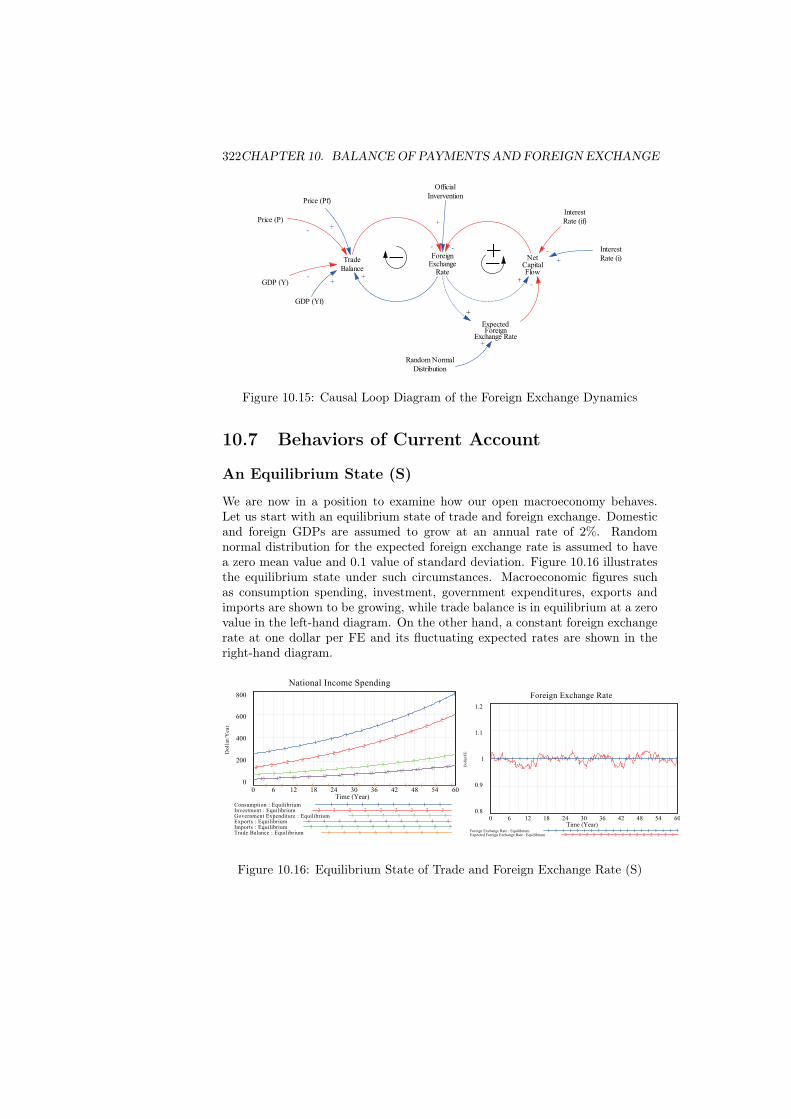
Figure 10.15: Causal Loop Diagram of the Foreign Exchange Dynamics
10.7 Behaviors of Current Account
An Equilibrium State (S)
We are now in a position to examine how our open macroeconomy behaves.Let us start with an equilibrium state of trade and foreign exchange. Domesticand foreign GDPs are assumed to grow at an annual rate of 2%. Randomnormal distribution for the expected foreign exchange rate is assumed to havea zero mean value and 0.1 value of standard deviation. Figure 10.16 illustratesthe equilibrium state under such circumstances. Macroeconomic figures suchas consumption spending, investment, government expenditures, exports andimports are shown to be growing, while trade balance is in equilibrium at a zerovalue in the left-hand diagram. On the other hand, a constant foreign exchangerate at one dollar per FE and its fluctuating expected rates are shown in theright-hand diagram.
National Income Spending
800
600
400
200
06 6 6 6 6 6 6 6 6 6 6 6 6
5 5 5 5 5 5 5 5 5 5 5 5 5
4 4 4 4 4 4 4 4 4 4 4 4 4
3 3 3 3 3 3 3 3 3 3 3 3 3
2 22
22
22
22
22
22
11
11
11
11
11
1
1
1
1
0 6 12 18 24 30 36 42 48 54 60Time (Year)
Do
llar
/Yea
r
Consumption : Equilibrium 1 1 1 1 1 1 1 1Investment : Equilibrium 2 2 2 2 2 2 2 2 2Government Expenditure : Equilibrium 3 3 3 3 3 3 3Exports : Equilibrium 4 4 4 4 4 4 4 4 4 4Imports : Equilibrium 5 5 5 5 5 5 5 5 5 5Trade Balance : Equilibrium 6 6 6 6 6 6 6 6
Foreign Exchange Rate
1.2
1.1
1
0.9
0.8
22 2
22 2
2
22 2 2
2
22
2 2 2
2 2
2 22
2 22 21 1 1 1 1 1 1 1 1 1 1 1 1 1 1 1 1 1 1 1 1 1 1 1 1 1 1
0 6 12 18 24 30 36 42 48 54 60Time (Year)
Doll
ar/F
E
Foreign Exchange Rate : Equilibrium 1 1 1 1 1 1 1 1 1 1 1 1 1 1 1 1 1 1 1Expected Foreign Exchange Rate : Equilibrium 2 2 2 2 2 2 2 2 2 2 2 2 2 2 2 2
Figure 10.16: Equilibrium State of Trade and Foreign Exchange Rate (S)
10.7. BEHAVIORS OF CURRENT ACCOUNT 323
In this state of equilibrium, financial investment is not yet considered. Hence,in spite of non-zero expected return arbitrate, caused by the fluctuations ofestimated foreign exchange rates, capital flows are not provoked, and accordinglytrade balance stays undisturbed.
Change in real GDP (S1)
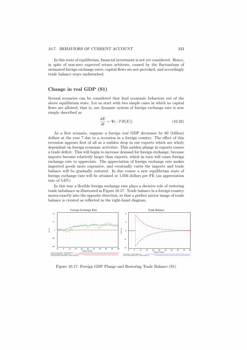
Several scenarios can be considered that lead economic behaviors out of theabove equilibrium state. Let us start with two simple cases in which no capitalflows are allowed; that is, our dynamic system of foreign exchange rate is nowsimply described as
dE
dt= Ψ(−TB(E)) (10.32)
As a first scenario, suppose a foreign real GDP decreases by 60 (billion)dollars at the year 7 due to a recession in a foreign country. The effect of thisrecession appears first of all as a sudden drop in our exports which are wholydependent on foreign economic activities. This sudden plunge in exports causesa trade deficit. This will begin to increase demand for foreign exchange, becauseimports become relatively larger than exports, which in turn will cause foreignexchange rate to appreciate. The appreciation of foreign exchange rate makesimported goods more expensive, and eventually curbs the imports and tradebalance will be gradually restored. In due course a new equilibrium state offoreign exchange rate will be attained at 1.056 dollars per FE (an appreciationrate of 5.6%)
In this way a flexible foreign exchange rate plays a decisive role of restoringtrade imbalance as illustrated in Figure 10.17. Trade balance in a foreign countrymoves exactly into the opposite direction, so that a perfect mirror image of tradebalance is created as reflected in the right-hand diagram.
Foreign Exchange Rate
1.2
1.1
1
0.9
0.8
33
3 3 3
3
3 3 3 3 33
33
3 3 3
33
33
33
3 3 3
2 2 2 2 2 2 2 2 2 2 2 2 2 2 2 2 2 2 2 2 2 2 2 2 2 21 1 1 11
1 1 1 1 1 1 1 1 1 1 1 1 1 1 1 1 1 1 1 1 1 1
0 6 12 18 24 30 36 42 48 54 60Time (Year)
Do
llar
/FE
Foreign Exchange Rate : GDP(f) Plunge(s1) 1 1 1 1 1 1 1 1 1 1 1 1 1 1 1 1 1Foreign Exchange Rate : Equilibrium 2 2 2 2 2 2 2 2 2 2 2 2 2 2 2 2 2 2Expected Foreign Exchange Rate : GDP(f) Plunge(s1) 3 3 3 3 3 3 3 3 3 3 3 3 3 3 3
Trade Balance
8
4
0
-4
-8
2 2 2
2
2
22
22
22 2 2 2 2 2 2 2 2 2 2 2 2 2 2 2 21 1 1
1
1
1
11
11
1 1 1 1 1 1 1 1 1 1 1 1 1 1 1 1 1
0 6 12 18 24 30 36 42 48 54 60Time (Year)
Do
llar
/Yea
r
Trade Balance : GDP(f) Plunge(s1) 1 1 1 1 1 1 1 1 1 1 1 1 1 1 1 1 1 1 1 1"Foreign Trade Balance (FE)" : GDP(f) Plunge(s1) 2 2 2 2 2 2 2 2 2 2 2 2 2 2 2
Figure 10.17: Foreign GDP Plunge and Restoring Trade Balance (S1)
324CHAPTER 10. BALANCE OF PAYMENTS AND FOREIGN EXCHANGE
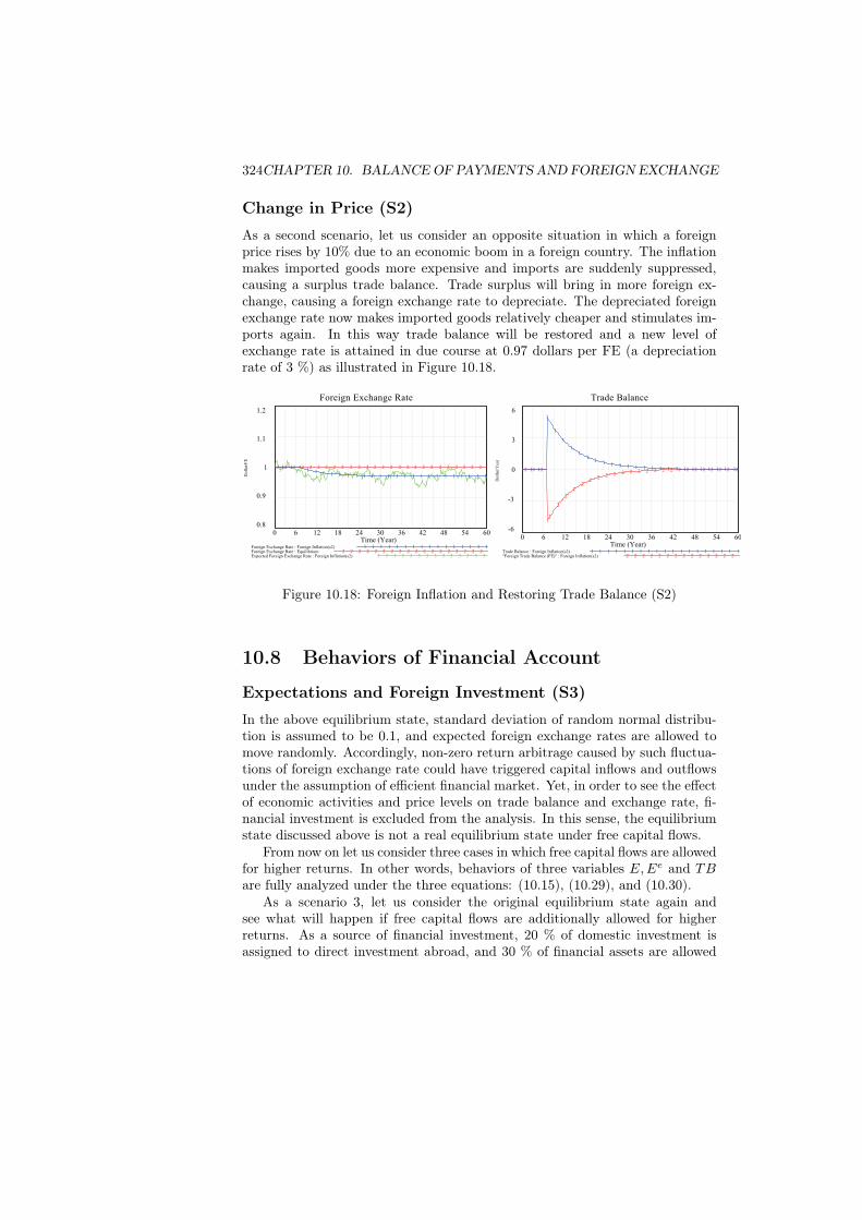
Change in Price (S2)As a second scenario, let us consider an opposite situation in which a foreignprice rises by 10% due to an economic boom in a foreign country. The inflationmakes imported goods more expensive and imports are suddenly suppressed,causing a surplus trade balance. Trade surplus will bring in more foreign ex-change, causing a foreign exchange rate to depreciate. The depreciated foreignexchange rate now makes imported goods relatively cheaper and stimulates im-ports again. In this way trade balance will be restored and a new level ofexchange rate is attained in due course at 0.97 dollars per FE (a depreciationrate of 3 %) as illustrated in Figure 10.18.
Foreign Exchange Rate
1.2
1.1
1
0.9
0.8
33
33
33
3 33 3
33
3 33 3 3
33
33
33
3 3 3
2 2 2 2 2 2 2 2 2 2 2 2 2 2 2 2 2 2 2 2 2 2 2 2 2 21 1 1 11 1 1 1 1 1 1 1 1 1 1 1 1 1 1 1 1 1 1 1 1 1 1
0 6 12 18 24 30 36 42 48 54 60Time (Year)
Do
llar
/FE
Foreign Exchange Rate : Foreign Inflation(s2) 1 1 1 1 1 1 1 1 1 1 1 1 1 1 1 1Foreign Exchange Rate : Equilibrium 2 2 2 2 2 2 2 2 2 2 2 2 2 2 2 2 2 2Expected Foreign Exchange Rate : Foreign Inflation(s2) 3 3 3 3 3 3 3 3 3 3 3 3 3 3
Trade Balance
6
3
0
-3
-6
2 2 2
2
2
2
22
22 2 2 2 2 2 2 2 2 2 2 2 2 2 2 2 2 21 1 1
1
1
1
11
11 1 1 1 1 1 1 1 1 1 1 1 1 1 1 1 1 1
0 6 12 18 24 30 36 42 48 54 60Time (Year)
Do
llar
/Yea
r
Trade Balance : Foreign Inflation(s2) 1 1 1 1 1 1 1 1 1 1 1 1 1 1 1 1 1 1 1"Foreign Trade Balance (FE)" : Foreign Inflation(s2) 2 2 2 2 2 2 2 2 2 2 2 2 2 2
Figure 10.18: Foreign Inflation and Restoring Trade Balance (S2)
10.8 Behaviors of Financial Account
Expectations and Foreign Investment (S3)In the above equilibrium state, standard deviation of random normal distribu-tion is assumed to be 0.1, and expected foreign exchange rates are allowed tomove randomly. Accordingly, non-zero return arbitrage caused by such fluctua-tions of foreign exchange rate could have triggered capital inflows and outflowsunder the assumption of efficient financial market. Yet, in order to see the effectof economic activities and price levels on trade balance and exchange rate, fi-nancial investment is excluded from the analysis. In this sense, the equilibriumstate discussed above is not a real equilibrium state under free capital flows.
From now on let us consider three cases in which free capital flows are allowedfor higher returns. In other words, behaviors of three variables E,Ee and TBare fully analyzed under the three equations: (10.15), (10.29), and (10.30).
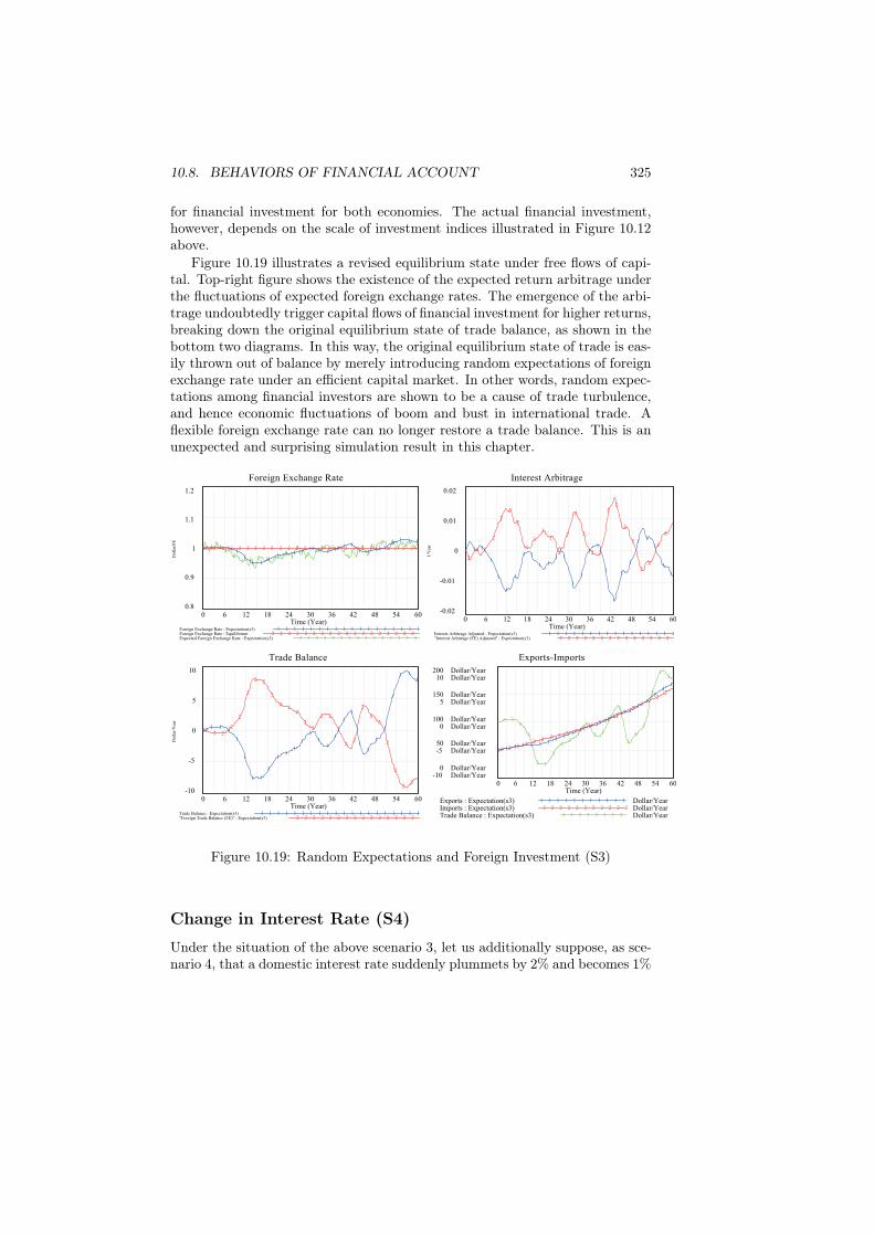
As a scenario 3, let us consider the original equilibrium state again andsee what will happen if free capital flows are additionally allowed for higherreturns. As a source of financial investment, 20 % of domestic investment isassigned to direct investment abroad, and 30 % of financial assets are allowed
10.8. BEHAVIORS OF FINANCIAL ACCOUNT 325
for financial investment for both economies. The actual financial investment,however, depends on the scale of investment indices illustrated in Figure 10.12above.
Figure 10.19 illustrates a revised equilibrium state under free flows of capi-tal. Top-right figure shows the existence of the expected return arbitrage underthe fluctuations of expected foreign exchange rates. The emergence of the arbi-trage undoubtedly trigger capital flows of financial investment for higher returns,breaking down the original equilibrium state of trade balance, as shown in thebottom two diagrams. In this way, the original equilibrium state of trade is eas-ily thrown out of balance by merely introducing random expectations of foreignexchange rate under an efficient capital market. In other words, random expec-tations among financial investors are shown to be a cause of trade turbulence,and hence economic fluctuations of boom and bust in international trade. Aflexible foreign exchange rate can no longer restore a trade balance. This is anunexpected and surprising simulation result in this chapter.
Foreign Exchange Rate
1.2
1.1
1
0.9
0.8
33
33
3 3 3 3 33 3
33
33 3 3
33
33
33
3 3 32 2 2 2 2 2 2 2 2 2 2 2 2 2 2 2 2 2 2 2 2 2 2 2 2 21 1 1 11
11 1
11 1 1 1 1 1 1 1
1 11 1 1 1
11 1 1
0 6 12 18 24 30 36 42 48 54 60Time (Year)
Do
llar
/FE
Foreign Exchange Rate : Expectation(s3) 1 1 1 1 1 1 1 1 1 1 1 1 1 1 1 1 1 1Foreign Exchange Rate : Equilibrium 2 2 2 2 2 2 2 2 2 2 2 2 2 2 2 2 2 2Expected Foreign Exchange Rate : Expectation(s3) 3 3 3 3 3 3 3 3 3 3 3 3 3 3 3
Interest Arbitrage
0.02
0.01
0
-0.01
-0.02
2
2 2
2
2
2
2
2
2
2
2
2
2
2
2
2 2
22
2
2
22
2
2
1 1 1
1
1
1
1
1 1
1 11 1
1
1
11
1
1
1
1
11
1
1
1
0 6 12 18 24 30 36 42 48 54 60Time (Year)
1/Y
ear
Interest Arbitrage Adjusted : Expectation(s3) 1 1 1 1 1 1 1 1 1 1 1 1 1 1 1 1"Interest Arbitrage (FE) Adjusted" : Expectation(s3) 2 2 2 2 2 2 2 2 2 2 2 2 2 2
Trade Balance
10
5
0
-5
-10
22 2
2
2
2
2 2
2
22
2
22
2 2
2
22
2
22
2
2
22
11 1
1
1
1
1 1
1
11
1
1
1
11
1
1
1
11
1
1
1
1 11
0 6 12 18 24 30 36 42 48 54 60Time (Year)
Do
llar
/Yea
r
Trade Balance : Expectation(s3) 1 1 1 1 1 1 1 1 1 1 1 1 1 1 1 1 1 1 1 1"Foreign Trade Balance (FE)" : Expectation(s3) 2 2 2 2 2 2 2 2 2 2 2 2 2 2 2
Exports-Imports
200 Dollar/Year10 Dollar/Year
150 Dollar/Year5 Dollar/Year
100 Dollar/Year0 Dollar/Year
50 Dollar/Year-5 Dollar/Year
0 Dollar/Year-10 Dollar/Year
3 33
3
3 3
3
33
3
3
3 3
3
3
3
3
3
3
33
2 2 2 2 2 2 2 2 2 22
22
22
22
22
22
1 1 1 1 1 1 11
11
11 1
11
1 11
11
11
0 6 12 18 24 30 36 42 48 54 60Time (Year)
Exports : Expectation(s3) Dollar/Year1 1 1 1 1 1 1 1 1 1 1
Imports : Expectation(s3) Dollar/Year2 2 2 2 2 2 2 2 2 2 2
Trade Balance : Expectation(s3) Dollar/Year3 3 3 3 3 3 3 3
Figure 10.19: Random Expectations and Foreign Investment (S3)
Change in Interest Rate (S4)
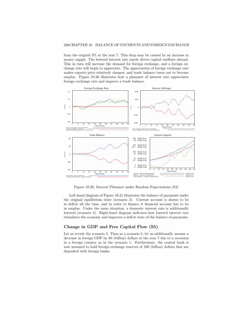
Under the situation of the above scenario 3, let us additionally suppose, as sce-nario 4, that a domestic interest rate suddenly plummets by 2% and becomes 1%
326CHAPTER 10. BALANCE OF PAYMENTS AND FOREIGN EXCHANGE
from the original 3% at the year 7. This drop may be caused by an increase inmoney supply. The lowered interest rate surely drives capital outflows abroad.This in turn will increase the demand for foreign exchange, and a foreign ex-change rate will begin to appreciate. The appreciation of foreign exchange ratemakes exports price relatively cheaper, and trade balance turns out to becomesurplus. Figure 10.20 illustrates how a plummet of interest rate appreciatesforeign exchange rate and improve a trade balance.
Foreign Exchange Rate
1.2
1.1
1
0.9
0.8
33
33
3
33 3 3
3 3
3 33 3 3 3
3 3 3 33
33 3
3
2 2 2 2 2 2 2 2 2 2 2 2 2 2 2 2 2 2 2 2 2 2 2 2 2 21 1 1 1 1 1 1 11
1 11
1 11 1
11 1
11 1 1
1 1 11
0 6 12 18 24 30 36 42 48 54 60Time (Year)
Do
llar
/FE
Foreign Exchange Rate : Interest Plummet(s4) 1 1 1 1 1 1 1 1 1 1 1 1 1 1 1 1 1Foreign Exchange Rate : Equilibrium 2 2 2 2 2 2 2 2 2 2 2 2 2 2 2 2 2 2Expected Foreign Exchange Rate : Interest Plummet(s4) 3 3 3 3 3 3 3 3 3 3 3 3 3 3
Interest Arbitrage
0.04
0.02
0
-0.02
-0.04
22 2 2
22
2
2 2 22
2
22
2
22
2 2
2
2
22
22
1 1 11 1
11
1 1 11 1 1
1
1
1 1
1
1
1
1
1 11
1 1
0 6 12 18 24 30 36 42 48 54 60Time (Year)
1/Y
ear
Interest Arbitrage Adjusted : Interest Plummet(s4) 1 1 1 1 1 1 1 1 1 1 1 1 1 1 1"Interest Arbitrage (FE) Adjusted" : Interest Plummet(s4) 2 2 2 2 2 2 2 2 2 2 2 2
Trade Balance
40
20
0
-20
-40
2 2 2 2 2 2 22
22 2
2
2 22
2
22
2
2 22
22 2
2
1 1 1 1 1 1 1 11
1 11
1 1 1 1
1
1 1
11
11
11 1
1
0 6 12 18 24 30 36 42 48 54 60Time (Year)
Do
llar
/Yea
r
Trade Balance : Interest Plummet(s4) 1 1 1 1 1 1 1 1 1 1 1 1 1 1 1 1 1 1 1"Foreign Trade Balance (FE)" : Interest Plummet(s4) 2 2 2 2 2 2 2 2 2 2 2 2 2 2
Exports-Imports
200 Dollar/Year40 Dollar/Year
150 Dollar/Year29.5 Dollar/Year
100 Dollar/Year19 Dollar/Year
50 Dollar/Year8.5 Dollar/Year
0 Dollar/Year-2 Dollar/Year
3 3 3 33
3
33
3
3 33
3
3
3
33
3
33
3
2 2 2 2 2 2 2 2 2 2 22
2 22
22
22
22
1 1 1 1 1 11
11
11
11
11 1 1
1
11
1
0 6 12 18 24 30 36 42 48 54 60Time (Year)
Exports : Interest Plummet(s4) Dollar/Year1 1 1 1 1 1 1 1 1 1 1 1Imports : Interest Plummet(s4) Dollar/Year2 2 2 2 2 2 2 2 2 2 2Trade Balance : Interest Plummet(s4) Dollar/Year3 3 3 3 3 3 3 3 3
Figure 10.20: Interest Plummet under Random Expectations (S4)
Left-hand diagram of Figure 10.21 illustrates the balance of payments underthe original equilibrium state (scenario 3). Current account is shown to bein deficit all the time, and in order to finance it financial account has to bein surplus. Under the same situation, a domestic interest rate is additionallylowered (scenario 4). Right-hand diagram indicates how lowered interest ratestimulates the economy and improves a deficit state of the balance of payments.
Change in GDP and Free Capital Flow (S5)Let us revisit the scenario 3. Then as a scenario 5, let us additionally assume adecrease in foreign GDP by 60 (billion) dollars at the year 7 due to a recessionin a foreign country as in the scenario 1. Furthermore, the central bank isnow assumed to hold foreign exchange reserves of 100 (billion) dollars that aredeposited with foreign banks.
10.8. BEHAVIORS OF FINANCIAL ACCOUNT 327
Balance of Payments
20
10
0
-10
-20
4 4 4 4 4 4 4 4 4 4 4 4 4 4 4 4 4 4 43 3 3 3 3 3 3 3 3 3 3 3 3 3 3 3 3 3 3 32 2 2
2
2 22
22
22
22
2
2 2
2
2
2
2
1 1 1
1
1 1 1 1 11
1
11
1 1
1
11
1 1
0 6 12 18 24 30 36 42 48 54 60Time (Year)
Do
llar
/Yea
r
Current Account : Expectation(s3) 1 1 1 1 1 1 1 1 1 1 1 1 1 1"Capital & Financial Account" : Expectation(s3) 2 2 2 2 2 2 2 2 2 2 2 2Change in Reserve Assets : Expectation(s3) 3 3 3 3 3 3 3 3 3 3 3 3 3Balance of Payments : Expectation(s3) 4 4 4 4 4 4 4 4 4 4 4 4 4
Balance of Payments
80
40
0
-40
-80
4 4 4 4 4 4 4 4 4 4 4 4 4 4 4 4 4 4 43 3 3 3 3 3 3 3 3 3 3 3 3 3 3 3 3 3 3 32 2 2 2 2 22
22 2
22 2
2
2 2
22
22
1 1 1 1 1 11 1 1
1 1
1 11
1 1
11
1
1
0 6 12 18 24 30 36 42 48 54 60Time (Year)
Do
llar
/Yea
r
Current Account : Interest Plummet(s4) 1 1 1 1 1 1 1 1 1 1 1 1 1"Capital & Financial Account" : Interest Plummet(s4) 2 2 2 2 2 2 2 2 2 2 2Change in Reserve Assets : Interest Plummet(s4) 3 3 3 3 3 3 3 3 3 3 3 3Balance of Payments : Interest Plummet(s4) 4 4 4 4 4 4 4 4 4 4 4 4
Figure 10.21: Comparison of the Balance of Payments between S3 and S4
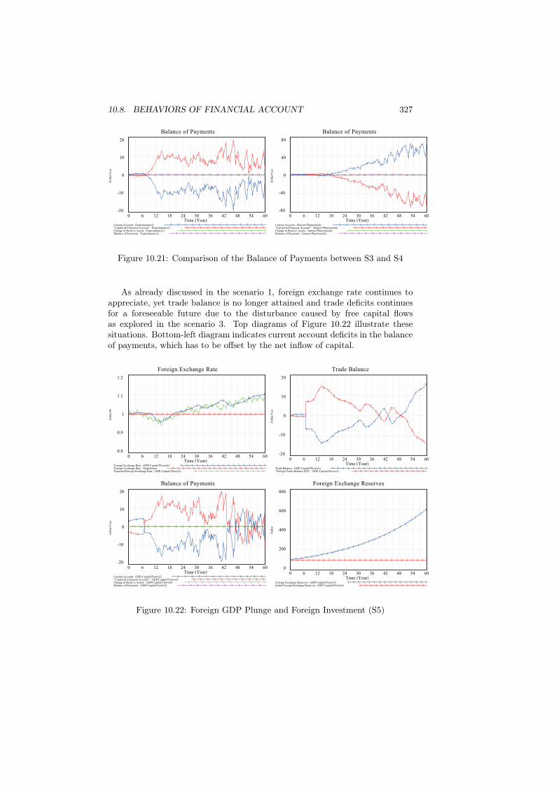
As already discussed in the scenario 1, foreign exchange rate continues toappreciate, yet trade balance is no longer attained and trade deficits continuesfor a foreseeable future due to the disturbance caused by free capital flowsas explored in the scenario 3. Top diagrams of Figure 10.22 illustrate thesesituations. Bottom-left diagram indicates current account deficits in the balanceof payments, which has to be offset by the net inflow of capital.
Foreign Exchange Rate
1.2
1.1
1
0.9
0.8
33
33
3 3 3 33
3 3
33
33 3 3
33
33
33 3
3 3
2 2 2 2 2 2 2 2 2 2 2 2 2 2 2 2 2 2 2 2 2 2 2 2 2 21 1 1 1 1
11
11
1 1 11
1 1 11
11
1 11 1
11 1 1
0 6 12 18 24 30 36 42 48 54 60Time (Year)
Do
llar
/FE
Foreign Exchange Rate : GDP-Capital Flow(s5) 1 1 1 1 1 1 1 1 1 1 1 1 1 1 1 1 1Foreign Exchange Rate : Equilibrium 2 2 2 2 2 2 2 2 2 2 2 2 2 2 2 2 2 2Expected Foreign Exchange Rate : GDP-Capital Flow(s5) 3 3 3 3 3 3 3 3 3 3 3 3 3 3
Trade Balance
20
10
0
-10
-20
2 2 2
22
22
2
22 2
22
2
2 2
2
2 2
2
22
2
2
22
1 1 1
1 1
1
11
1
11
11
11
1
1
1
1
11
11
1
11
1
0 6 12 18 24 30 36 42 48 54 60Time (Year)
Do
llar
/Yea
r
Trade Balance : GDP-Capital Flow(s5) 1 1 1 1 1 1 1 1 1 1 1 1 1 1 1 1 1 1 1"Foreign Trade Balance (FE)" : GDP-Capital Flow(s5) 2 2 2 2 2 2 2 2 2 2 2 2 2 2
Balance of Payments
20
10
0
-10
-20
4 4 4 4 4 4 4 4 4 4 4 4 4 4 4 4 4 4 43 3 3 3 3 3 3 3 3 3 3 3 3 3 3 3 3 3 3 3
2 2
22
22
2
2
2
2
2
2
2
2
22
22
2
211 1
1
11 1 1 1
1
1
1
1
1
1
1
1
1
1
1
0 6 12 18 24 30 36 42 48 54 60Time (Year)
Do
llar
/Yea
r
Current Account : GDP-Capital Flow(s5) 1 1 1 1 1 1 1 1 1 1 1 1 1"Capital & Financial Account" : GDP-Capital Flow(s5) 2 2 2 2 2 2 2 2 2 2 2Change in Reserve Assets : GDP-Capital Flow(s5) 3 3 3 3 3 3 3 3 3 3 3 3Balance of Payments : GDP-Capital Flow(s5) 4 4 4 4 4 4 4 4 4 4 4 4
Foreign Exchange Reserves
800
600
400
200
0
2 2 2 2 2 2 2 2 2 2 2 2 2 2 2 2 2 2 2 2 2 2 2 2 2 21 1 1 1 1 1 1 1 1 1 1 1 1 11
11
11
11
11
11
11
0 6 12 18 24 30 36 42 48 54 60Time (Year)
Do
llar
Foreign Exchange Reserves : GDP-Capital Flow(s5) 1 1 1 1 1 1 1 1 1 1 1 1 1 1 1 1Initial Foreign Exchange Reserves : GDP-Capital Flow(s5) 2 2 2 2 2 2 2 2 2 2 2 2 2
Figure 10.22: Foreign GDP Plunge and Foreign Investment (S5)
328CHAPTER 10. BALANCE OF PAYMENTS AND FOREIGN EXCHANGE
Bottom-right diagram shows that foreign exchange reserves by the centralbank continues to grow at a rate of the foreign interest rate of 3 %. From awell-known principle of a doubling time of exponential growth, the reserves keepdoubling approximately every 23 years.
10.9 Foreign Exchange Intervention
Official Intervention and Default (S6)
In the scenario 5 above, our macroeconomy continues to suffer from a continualdepreciation of domestic currency (or an appreciation of foreign exchange rate),and deficits in trade and accordingly in current account. Surely, such a criticalmacroeconomic situation in a competitive international economic environmentcannot be left uncontrolled. To prevent such an economic crisis let us introduce,as scenario 6, an official intervention to the foreign exchange market; specifically,the central bank (and government) begins to sell foreign exchange in order toreduce foreign exchange rate, say, to 1.02 dollars per FE; that is, by 2 % of theoriginal equilibrium exchange rate.
As Figure 10.23 illustrates, even under such circumstances trade and currentaccount deficits continue to persist. Gradually, the foreign exchange reservesbegins to decline due to the official intervention, and becomes lower than theoriginal reserve level of 100 (billion) dollars around the year 40 and completelygets depleted around the year 50, as indicated in the bottom right-hand diagram.This implies the government is forced to declare financial default, that is, aneconomic destruction, unless successfully eliciting an emergent loan from theinternational institutions such as the IMF.
Zero Interest Rate and Default (S7)
To avoid such financial default, now suppose, as scenario 7, money supply isincreased to stimulate the economy and a domestic interest rate is lowered by3%; that is, a zero interest rate is introduced from the original 3% at the year 3.This policy of zero interest rate surely improves trade balance and the balanceof payments as Figure 10.24 indicates. Yet, under the official intervention ofkeeping a foreign exchange rate below 1.02 dollars per FE, the central bank (andthe government) is forced to keep selling foreign exchange reserves3. The original100 (billion) dollars of foreign exchange reserves will be completely depletedaround the year 11 as the bottom right-hand diagram indicates. Therefore, thiszero interest policy does not work unless the government can successfully borrowforeign exchange from the international institutions such as the IMF.
3To be precise, for maintaining the rate below this level, the central bank (and the gov-ernment) has to keep selling 60 (billion) dollars of foreign exchange annually instead of 20(billion) dollars in the previous scenario
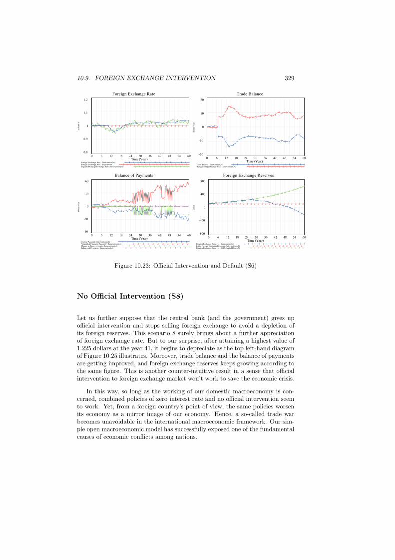
10.9. FOREIGN EXCHANGE INTERVENTION 329
Foreign Exchange Rate
1.2
1.1
1
0.9
0.8
33
33
3 3 3 33
3 3
33 3
3 3 3
33
33
33
3 3 32 2 2 2 2 2 2 2 2 2 2 2 2 2 2 2 2 2 2 2 2 2 2 2 2 21 1 1 1 1
11
11
1 1 1 1 1 1 1 1 1 1 1 1 1 11 1 1 1
0 6 12 18 24 30 36 42 48 54 60Time (Year)
Do
llar
/FE
Foreign Exchange Rate : Intervention(s6) 1 1 1 1 1 1 1 1 1 1 1 1 1 1 1 1 1 1Foreign Exchange Rate : Equilibrium 2 2 2 2 2 2 2 2 2 2 2 2 2 2 2 2 2 2Expected Foreign Exchange Rate : Intervention(s6) 3 3 3 3 3 3 3 3 3 3 3 3 3 3 3
Trade Balance
20
10
0
-10
-20
2 2 2
22
22
2
22 2 2 2 2 2 2 2 2
22 2 2 2
22
2
1 1 1
1 1
1
11
1
11
1 1 1 1 1 1 1 11 1 1 1
1
1 11
0 6 12 18 24 30 36 42 48 54 60Time (Year)
Do
llar
/Yea
r
Trade Balance : Intervention(s6) 1 1 1 1 1 1 1 1 1 1 1 1 1 1 1 1 1 1 1 1"Foreign Trade Balance (FE)" : Intervention(s6) 2 2 2 2 2 2 2 2 2 2 2 2 2 2 2
Balance of Payments
60
30
0
-30
-60
4 4 4 4 4 4 4 4 4 4 4 4 4 4 4 4 4 4 43 3 3 3 3 3 3 3 3 3 3
3 3 3
3 3
3 3 3 3
2 2
2 22 2
22
22
22
2
2
2
22 2
2
2
1 1 1
1
1 1 1 1 1 1
1
1 1
1 1 1
11 1 1
0 6 12 18 24 30 36 42 48 54 60Time (Year)
Do
llar
/Yea
r
Current Account : Intervention(s6) 1 1 1 1 1 1 1 1 1 1 1 1 1 1"Capital & Financial Account" : Intervention(s6) 2 2 2 2 2 2 2 2 2 2 2 2Change in Reserve Assets : Intervention(s6) 3 3 3 3 3 3 3 3 3 3 3 3 3Balance of Payments : Intervention(s6) 4 4 4 4 4 4 4 4 4 4 4 4 4
Foreign Exchange Reserves
800
400
0
-400
-800
3 3 3 3 3 3 3 3 3 3 3 3 3 3 3 3 3 3 3 3 3 33
33
3
2 2 2 2 2 2 2 2 2 2 2 2 2 2 2 2 2 2 2 2 2 2 2 2 2 21 1 1 1 1 1 1 1 1 1 1 1 1 1 1 1 11
1 1 1 11
11
1
0 6 12 18 24 30 36 42 48 54 60Time (Year)
Do
llar
Foreign Exchange Reserves : Intervention(s6) 1 1 1 1 1 1 1 1 1 1 1 1 1 1 1 1 1Initial Foreign Exchange Reserves : Intervention(s6) 2 2 2 2 2 2 2 2 2 2 2 2 2 2Foreign Exchange Reserves : GDP-Capital Flow(s5) 3 3 3 3 3 3 3 3 3 3 3 3 3 3 3
Figure 10.23: Official Intervention and Default (S6)
No Official Intervention (S8)
Let us further suppose that the central bank (and the government) gives upofficial intervention and stops selling foreign exchange to avoid a depletion ofits foreign reserves. This scenario 8 surely brings about a further appreciationof foreign exchange rate. But to our surprise, after attaining a highest value of1.225 dollars at the year 41, it begins to depreciate as the top left-hand diagramof Figure 10.25 illustrates. Moreover, trade balance and the balance of paymentsare getting improved, and foreign exchange reserves keeps growing according tothe same figure. This is another counter-intuitive result in a sense that officialintervention to foreign exchange market won’t work to save the economic crisis.
In this way, so long as the working of our domestic macroeconomy is con-cerned, combined policies of zero interest rate and no official intervention seemto work. Yet, from a foreign country’s point of view, the same policies worsenits economy as a mirror image of our economy. Hence, a so-called trade warbecomes unavoidable in the international macroeconomic framework. Our sim-ple open macroeconomic model has successfully exposed one of the fundamentalcauses of economic conflicts among nations.
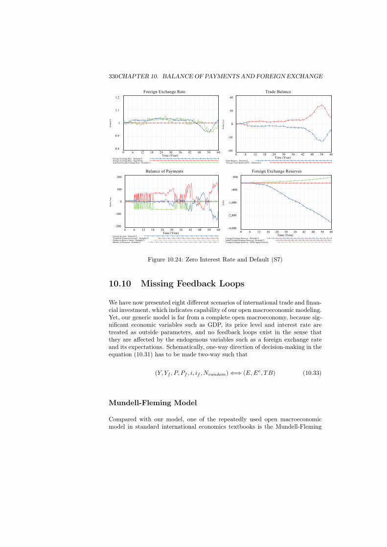
330CHAPTER 10. BALANCE OF PAYMENTS AND FOREIGN EXCHANGE
Foreign Exchange Rate
1.2
1.1
1
0.9
0.8
33
3 33
33 3 3 3
33
3 3 3 3 3
33
3 33
3
3 3
3
2 2 2 2 2 2 2 2 2 2 2 2 2 2 2 2 2 2 2 2 2 2 2 2 2 21 1 11 1 1 1 1 1 1 1 1 1 1
1 1 1 1 1 11
1
11
1
1
1
0 6 12 18 24 30 36 42 48 54 60Time (Year)
Do
llar
/FE
Foreign Exchange Rate : Default(s7) 1 1 1 1 1 1 1 1 1 1 1 1 1 1 1 1 1 1 1Foreign Exchange Rate : Equilibrium 2 2 2 2 2 2 2 2 2 2 2 2 2 2 2 2 2 2Expected Foreign Exchange Rate : Default(s7) 3 3 3 3 3 3 3 3 3 3 3 3 3 3 3 3
Trade Balance
60
30
0
-30
-60
2 2 2
2 2 2 2 2 2 2 2 2 2 2 2 2 2 2 22
2
2
22
2
2
1 1 11 1 1 1 1 1 1 1 1 1 1 1 1 1 1 1 1
11
11 1
1
1
0 6 12 18 24 30 36 42 48 54 60Time (Year)
Do
llar
/Yea
r
Trade Balance : Default(s7) 1 1 1 1 1 1 1 1 1 1 1 1 1 1 1 1 1 1 1 1 1"Foreign Trade Balance (FE)" : Default(s7) 2 2 2 2 2 2 2 2 2 2 2 2 2 2 2 2 2
Balance of Payments
200
100
0
-100
-200
4 4 4 4 4 4 4 4 4 4 4 4 4 4 4 4 4 4 43 3
3
3 3
3 3 3 3 3
3 3
3
3 3 3 3 3 32 2 2 2
2
2
2 22
2
2 2 2
2
2 2
2
2
2
2
1 1 1 1 1 1 1 1 1 11
1 1
1
1
1
1
1
1
1
0 6 12 18 24 30 36 42 48 54 60Time (Year)
Do
llar
/Yea
r
Current Account : Default(s7) 1 1 1 1 1 1 1 1 1 1 1 1 1 1 1"Capital & Financial Account" : Default(s7) 2 2 2 2 2 2 2 2 2 2 2 2 2Change in Reserve Assets : Default(s7) 3 3 3 3 3 3 3 3 3 3 3 3 3 3Balance of Payments : Default(s7) 4 4 4 4 4 4 4 4 4 4 4 4 4 4
Foreign Exchange Reserves
800
-400
-1,600
-2,800
-4,000
3 3 3 3 3 3 3 3 3 3 3 3 3 3 3 3 3 3 3 3 3 3 3 3 3
2 2 2 2 2 2 2 2 2 2 2 2 2 2 2 2 2 2 2 2 2 2 2 2 21 1 1 1 1 1 1 11
11
11
11
11
11
11
11
11
0 6 12 18 24 30 36 42 48 54 60Time (Year)
Do
llar
Foreign Exchange Reserves : Default(s7) 1 1 1 1 1 1 1 1 1 1 1 1 1 1 1 1 1 1Initial Foreign Exchange Reserves : Default(s7) 2 2 2 2 2 2 2 2 2 2 2 2 2 2 2Foreign Exchange Reserves : GDP-Capital Flow(s5) 3 3 3 3 3 3 3 3 3 3 3 3 3 3 3
Figure 10.24: Zero Interest Rate and Default (S7)
10.10 Missing Feedback Loops
We have now presented eight different scenarios of international trade and finan-cial investment, which indicates capability of our open macroeconomic modeling.Yet, our generic model is far from a complete open macroeconomy, because sig-nificant economic variables such as GDP, its price level and interest rate aretreated as outside parameters, and no feedback loops exist in the sense thatthey are affected by the endogenous variables such as a foreign exchange rateand its expectations. Schematically, one-way direction of decision-making in theequation (10.31) has to be made two-way such that
(Y, Yf , P, Pf , i, if , Nrandom) ⇐⇒ (E,Ee, TB) (10.33)
Mundell-Fleming Model
Compared with our model, one of the repeatedly used open macroeconomicmodel in standard international economics textbooks is the Mundell-Fleming
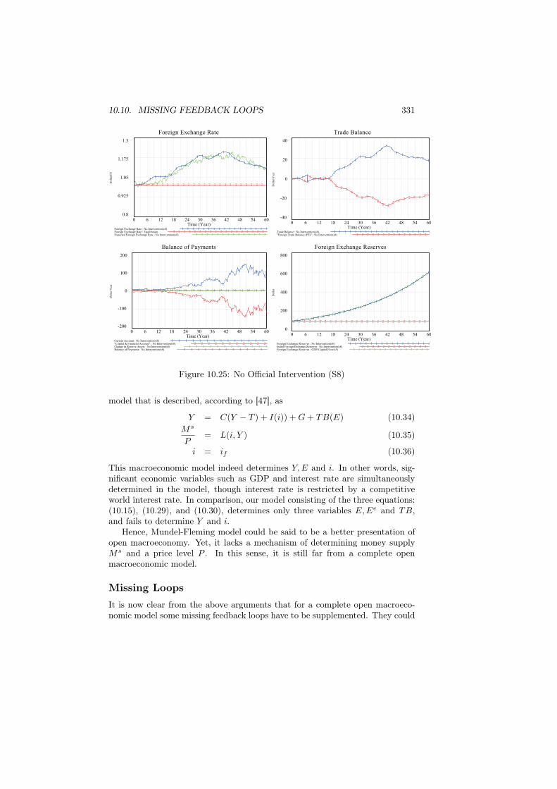
10.10. MISSING FEEDBACK LOOPS 331
Foreign Exchange Rate
1.3
1.175
1.05
0.925
0.8
33 3 3
3
33 3
33
33 3
33 3
3 33
3 3
3 3
33
2 2 2 2 2 2 2 2 2 2 2 2 2 2 2 2 2 2 2 2 2 2 2 2 21 1 11
1 1 11
11
11
1 11 1
11 1
11
1 1 1 11
0 6 12 18 24 30 36 42 48 54 60Time (Year)
Do
llar
/FE
Foreign Exchange Rate : No Intervention(s8) 1 1 1 1 1 1 1 1 1 1 1 1 1 1 1 1 1Foreign Exchange Rate : Equilibrium 2 2 2 2 2 2 2 2 2 2 2 2 2 2 2 2 2 2Expected Foreign Exchange Rate : No Intervention(s8) 3 3 3 3 3 3 3 3 3 3 3 3 3 3
Trade Balance
40
20
0
-20
-40
2 22
2 2 2 22
22 2
22
2 2 22
2 22
22 2 2 2 2
1 1 11
1 1 1 1
11 1
11
1 1 11
11
1
11
1 1 1 11
0 6 12 18 24 30 36 42 48 54 60Time (Year)
Do
llar
/Yea
r
Trade Balance : No Intervention(s8) 1 1 1 1 1 1 1 1 1 1 1 1 1 1 1 1 1 1 1"Foreign Trade Balance (FE)" : No Intervention(s8) 2 2 2 2 2 2 2 2 2 2 2 2 2 2
Balance of Payments
200
100
0
-100
-200
4 4 4 4 4 4 4 4 4 4 4 4 4 4 4 4 4 4 43 3 3 3 3 3 3 3 3 3 3 3 3 3 3 3 3 3 32 2 2 2 2 2 22 2 2
2 2 22
2 2
22
22
1 1 1 1 1 1 1 1 1 11
1 1
1
11
11
11
0 6 12 18 24 30 36 42 48 54 60Time (Year)
Do
llar
/Yea
r
Current Account : No Intervention(s8) 1 1 1 1 1 1 1 1 1 1 1 1 1 1"Capital & Financial Account" : No Intervention(s8) 2 2 2 2 2 2 2 2 2 2 2Change in Reserve Assets : No Intervention(s8) 3 3 3 3 3 3 3 3 3 3 3 3Balance of Payments : No Intervention(s8) 4 4 4 4 4 4 4 4 4 4 4 4
Foreign Exchange Reserves
800
600
400
200
0
3 3 3 3 3 3 3 3 3 3 3 3 33
33
33
33
33
33
33
2 2 2 2 2 2 2 2 2 2 2 2 2 2 2 2 2 2 2 2 2 2 2 2 2 21 1 1 1 1 1 1 1 1 1 1 1 1 11
11
11
11
11
11
11
0 6 12 18 24 30 36 42 48 54 60Time (Year)
Do
llar
Foreign Exchange Reserves : No Intervention(s8) 1 1 1 1 1 1 1 1 1 1 1 1 1 1 1 1Initial Foreign Exchange Reserves : No Intervention(s8) 2 2 2 2 2 2 2 2 2 2 2 2 2Foreign Exchange Reserves : GDP-Capital Flow(s5) 3 3 3 3 3 3 3 3 3 3 3 3 3 3 3
Figure 10.25: No Official Intervention (S8)
model that is described, according to [47], as
Y = C(Y − T ) + I(i)) +G+ TB(E) (10.34)Ms
P= L(i, Y ) (10.35)
i = if (10.36)
This macroeconomic model indeed determines Y,E and i. In other words, sig-nificant economic variables such as GDP and interest rate are simultaneouslydetermined in the model, though interest rate is restricted by a competitiveworld interest rate. In comparison, our model consisting of the three equations:(10.15), (10.29), and (10.30), determines only three variables E,Ee and TB,and fails to determine Y and i.
Hence, Mundel-Fleming model could be said to be a better presentation ofopen macroeconomy. Yet, it lacks a mechanism of determining money supplyMs and a price level P . In this sense, it is still far from a complete openmacroeconomic model.
Missing LoopsIt is now clear from the above arguments that for a complete open macroeco-nomic model some missing feedback loops have to be supplemented. They could
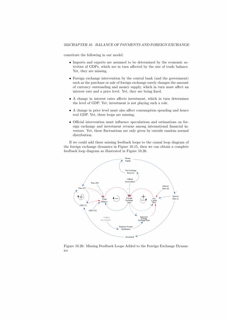
332CHAPTER 10. BALANCE OF PAYMENTS AND FOREIGN EXCHANGE
constitute the following in our model:
• Imports and exports are assumed to be determined by the economic ac-tivities of GDPs, which are in turn affected by the size of trade balance.Yet, they are missing.
• Foreign exchange intervention by the central bank (and the government)such as the purchase or sale of foreign exchange surely changes the amountof currency outstanding and money supply, which in turn must affect aninterest rate and a price level. Yet, they are being fixed.
• A change in interest rates affects investment, which in turn determinesthe level of GDP. Yet, investment is not playing such a role.
• A change in price level must also affect consumption spending and hencereal GDP. Yet, these loops are missing.
• Official intervention must influence speculations and estimations on for-eign exchange and investment returns among international financial in-vestors. Yet, these fluctuations are only given by outside random normaldistribution.
If we could add these missing feedback loops to the causal loop diagram ofthe foreign exchange dynamics in Figure 10.15, then we can obtain a completefeedback loop diagram as illustrated in Figure 10.26.
GDP (Y)
TradeBalance
ForeignExchange
Rate-
-
+
Random NormalDistribution
ExpectedForeign
Exchange Rate+
NetCapitalFlow
-
-
+
InterestRate (i)+
Price (P)
-
OfficialInvervention
+
+
GDP (Yf)
Price (Pf)
InterestRate (if)
+
+
-
Net ExchangeReserves
MoneySupply
+
+
+
+
Investment +
+
+
+
<OfficialInvervention>
+
Figure 10.26: Missing Feedback Loops Added to the Foreign Exchange Dynam-ics
10.11. CONCLUSION 333
Obviously, our open macroeconomic model is not complete until these miss-ing loops are incorporated in the model. Specifically, the previous chapter haspresented a model of macroeconomic system which determines GDP, money sup-ply, a price level, investment and interest rate, to name but a few. Therefore,our next challenge is to integrate the model with our present foreign exchangemodel by creating a whole image of domestic macroeconomy as its foreign sectormacroeconomy.
10.11 ConclusionOur open macroeconomic modeling turned out to need another model of thebalance of payments and dynamics of foreign exchange rate. Consequently, theapproach in this chapter led by the logic of accounting system dynamics becamean entirely new one in the field of international economics.
Under the framework, a double-booking accounting of the balance of pay-ments is modeled. Then determinants of trade and foreign direct and financialinvestment are analytically examined together with an introduction of differen-tial equations of foreign exchange rate and its expected rate.
Upon a completion of the model, eight scenarios are produced and exam-ined by running various simulations to obtain some behaviors observed in actualinternational trade and financial investment. It is a surprise to see how an equi-librium state of trade balance is easily disturbed by merely introducing randomexpectations among financial investors under the assumption of efficient finan-cial market. To indicate the capability of our model furthermore, the impact ofofficial intervention on foreign exchange and a path to default is discussed.
Finally, several missing feedback loops in our model are pointed out formaking it a complete open macroeconomic model. This task of completion willinevitably lead to our next research in this system dynamics macroeconomicmodeling series in the next chapter.


![767 INDEX [] · 767 INDEX ... index](https://img.pdfslide.us/doc/110x75/5e6407d785e377181b6fee19/767-index-767-index-index-.jpg)

![INDEX [] · 2019-04-15 · INDEX ... index](https://img.pdfslide.us/doc/110x75/5e5bc6adf543e8499e5ad9a4/index-2019-04-15-index-index.jpg)
![index [] · index ... index](https://img.pdfslide.us/doc/110x75/5e33c50d475fc05b6d5265f9/index-index-index.jpg)
