Embed Size (px)
Citation preview
NOTES ON OPEN CHANNEL FLOW
Profili di moto
permanente in un
canale e in una serie
di due canali -
Boudine, 1861
Prof. Marco Pilotti
Facoltà di Ingegneria, Università
degli Studi di Brescia

OPEN CHANNEL FLOW: glossary and main symbols used during the lectures
M. Pilotti - lectures of Environmental Hydraulics
Proprietà dei fluidi
Fluid properties
g : [m/s2] accelerazione di gravità gravity acceleration
γ : [N/m3] peso specifico del fluido Fluid specific weight
ρ : [Kg/m3] densità di massa del fluido Fluid mass density
µ : [Ns/m2] primo coefficiente di viscosità dinamica Viscosity coefficient
ν : [m2/s] coefficiente di viscosità cinematica Kinematic viscosity coefficient
Proprietà generali del moto
General properties
h : [m] altezza della corrente Water depth R : [m] raggio idraulico Hydraulic radius P : [m] perimetro bagnato Wetted perimeter U : [m/s] velocità media della corrente Average flow velocity Q : [m3/s] portata liquida Liquid volumetric discharge u : [m/s] velocità puntuale della corrente Local flow velocity v* : [m/s] velocità d'attrito Shear velocity
bS : [-] pendenza del fondo dell’alveo Bed slope
fS : [-] cadente totale Slope friction, Head slope
wS : [-] pendenza del pelo libero Water surface slope
q : [m2/s] portata liquida in volume per unità di larghezza dell’alveo Liquid volumetric discharge per unit length qi : [m2/s] portata in volume entrante per unità di lunghezza dell’alveo As above, entering the flow qo : [m2/s] portata in volume uscente per unità di lunghezza dell’alveo As above, going out of the flow
τ : [N/m2] sforzo superficiale Shear stress
τ0 : [N/m2] sforzo medio al fondo Average bed shear stress

OPEN CHANNEL FLOW: glossary and main symbols used during the lectures
M. Pilotti - lectures of Environmental Hydraulics
Proprietà generali del moto
General properties
z+p/γ : [m] carico piezometrico Piezometric pressure
Linea dei carichi totali Total energy line Linea dei carichi piezometrici Hydraulic grade line S : [N] Spinta totale della corrente Specific Force
h0 : [m] Profondità di moto uniforme Normal depth A : [mq] Area bagnata della sezione retta Wetted surface B : [m] Larghezza della sezione Top width of the wetted surface D : [m] Profondità media della corrente = A(h)/B(h) Hydraulic depth Q(h) Scala delle portate Stage-discharge relationship Termini generali
Words of common usage
bonifica Land reclamation fognatura sewer rigurgito swellhead Altezze coniugate sequent depths or conjugate depths

OPEN CHANNEL FLOW: glossary and main symbols used during the lectures
M. Pilotti - lectures of Environmental Hydraulics
Numeri adimensionali
Dimensionless groups
Fr =U
gh
Numero di Froude Froude number
Re=4UR
υ numero di Reynolds della corrente Reynolds number
X =ρ
µv D*
numero di Reynolds del fondo grain Reynolds number
Y =ργ
v
Ds
*2
numero di mobilità (sforzo adimensionale al fondo) Dimensionless shear stress (mobility
number)
ΠA generica versione adimensionale di una propietà A del moto bifase
Dimensionless number corresponding to dimensional property A
OPEN CHANNEL FLOW: basic assumptions
M. Pilotti - lectures of Environmental Hydraulics
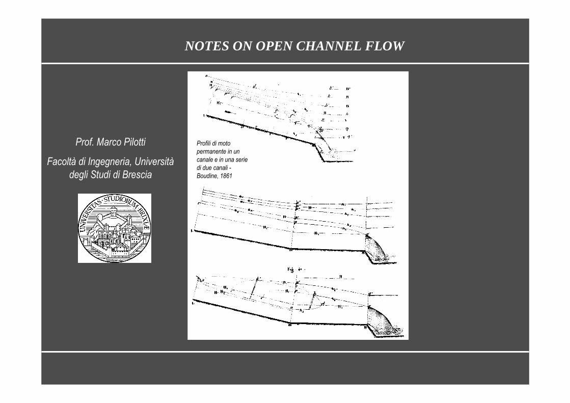
Free surface flow: the upper surface is limited by a gas (tipically, the atmosphere) so that its pressure is constant
Tipical cases: channel (irrigation, hydropower supply, water supply, land reclamation…) river, sewer conduits, lakes…
Particular cases: groundwater flow, free surface flow in a syphon
Main hypothesis in these lectures
• 1D approach in steady conditions
• Single-phase flow in unerodible, fixed bed
• Newtonian, constant density fluid
• Mostly, linear flow in rough turbulent conditions
• Bed slope if < 0.1 m/m
Minimum slope Maximum slope Irrigation or land reclamation channel 0.0001 0.001 Sewer free surface pipe 0.001 0.05 Floodplain river 0.00005 0.005 creek 0.005 0.3
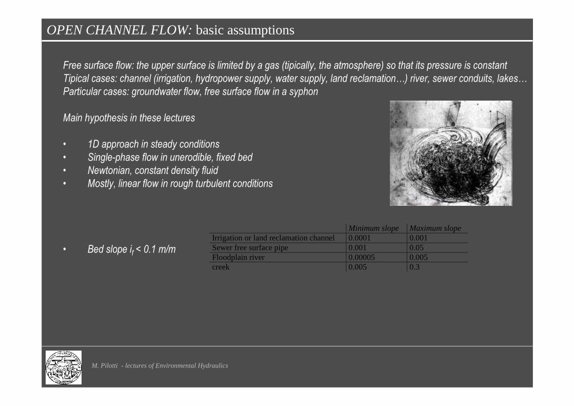
OPEN CHANNEL FLOW: typical slopes
M. Pilotti - lectures of Environmental Hydraulics
500
700
900
1100
1300
1500
0 300 600 900 1200 1500 1800 2100 2400 2700 3000
s [m]
z [m
]
20
25
30
35
40
45
50
55
60
pen
den
za [
%]
Profilo altimetrico
Pendenza media
Mississippi river between St. Louis and Minneapolis
(U.S. Corps of Engineers)
Typical mountain creek in Italian alps
(T. Rossiga, A = 3.72 Km2)

OPEN CHANNEL FLOW: relevance and applicability of basic hypothesis
M. Pilotti - lectures of Environmental Hydraulics
Unerodible and fixed bed: the area surrounding Isola Pescaroli
(from braided river to a single bed river)
OPEN CHANNEL FLOW: relevance and applicability of basic hypothesis
M. Pilotti - lectures of Environmental Hydraulics
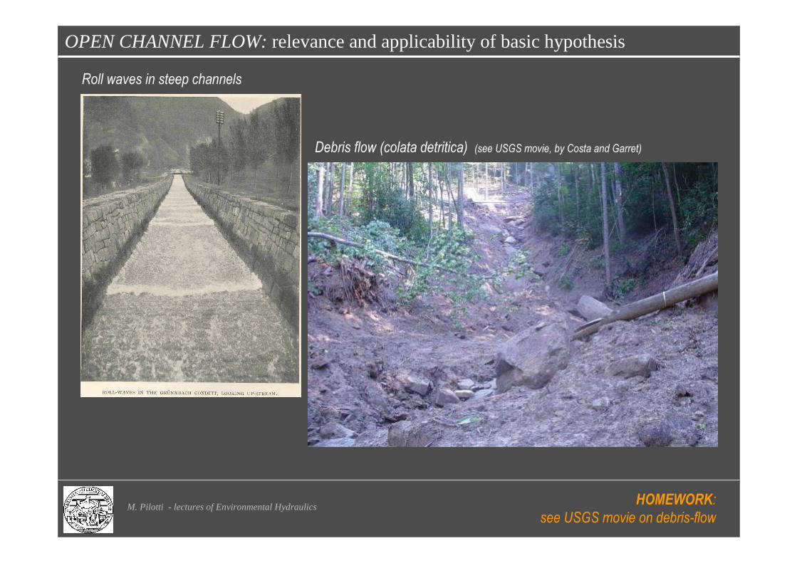
Roll waves in steep channels
Debris flow (colata detritica) (see USGS movie, by Costa and Garret)
HOMEWORK:
see USGS movie on debris-flow
OPEN CHANNEL FLOW: mass balance
M. Pilotti - lectures of Environmental Hydraulics
Mass balance for a control volume
M
A
QdAnV =⋅∫ )(rr
ρ Mass discharge through A, the
area of the cross section
QQdAnV V
S
==⋅∫rr
A
dAS∫
=ρ
ρAverage density on A
A
QU M
ρ= Average velocity on A
dxx
UAdxxQxQdx
t
AMM ∂
∂=+−=∂
∂ )()()(
)( ρρ
0)()( =
∂∂+
∂∂
x
UA
t
A ρρ
Volumetric discharge through A
qx
UA
t
A =∂
∂+∂
∂ )()(
outin
A
QQdAnVdt
dW −=⋅= ∫ )(rr
(G.1) Mass balance for a basin, under constant density
assumption
Mass balance for 1D flow
0)()()( =⋅−∂∂= ∫∫∫
AWW
dAnVdWt
dWDt
D rrρρρ
(G.1a) Mass balance for 1D flow when density varies (e.g.,turbiditic flow
or debris flow)
(G.1b) Mass balance for 1D flow when density is constant (typically, in
open channel flow), and with net discharge q per unit length
HOMEWORK:
see exercises on Sarnico dam and on dam breach

OPEN CHANNEL FLOW: energy balance
M. Pilotti - lectures of Environmental Hydraulics
First and second
Coriolis’ coefficient
(G.2) Energy balance equation for 1D gradually unsteady varied flow
(G.2a) Total head
(G.2b) Specific Energy with respect to the thalweg
Relationship between (G.2a) and (G.2b)
(G.2c) Energy balance in terms of E
fSt
U
gs
H −∂
∂−=∂∂ β
g
Uhz
g
UpzH
22
22 ααγ
++=++=
AU
dAu
AU
dAu
A
A
2
2
3
3
;
∫
∫
=
=
β
α
t
U
gSS
s
Es
ES
s
E
s
z
s
H
Ezg
UhzH
fb
b
∂∂−−=
∂∂
∂∂+−=
∂∂+
∂∂=
∂∂
+=++=
β
α2
2
2
22
)(22 hgA
Qh
g
UhE
αα +=+=
fb SSds
dE −= (G.2d) Energy balance in terms of E in steady state
conditions
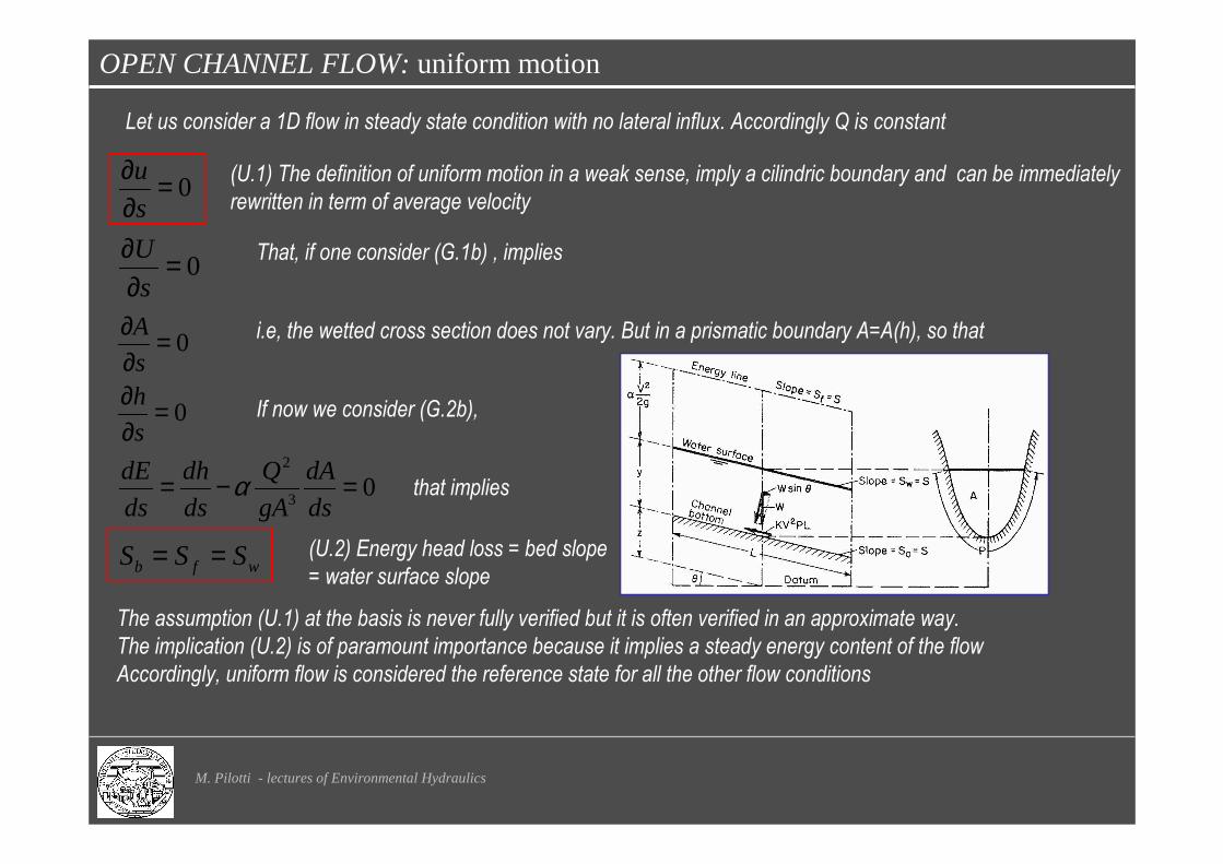
OPEN CHANNEL FLOW: uniform motion
M. Pilotti - lectures of Environmental Hydraulics
If now we consider (G.2b),
(U.1) The definition of uniform motion in a weak sense, imply a cilindric boundary and can be immediately
rewritten in term of average velocity
That, if one consider (G.1b) , implies
(U.2) Energy head loss = bed slope
= water surface slope
0=∂∂s
u
The assumption (U.1) at the basis is never fully verified but it is often verified in an approximate way.
The implication (U.2) is of paramount importance because it implies a steady energy content of the flow
Accordingly, uniform flow is considered the reference state for all the other flow conditions
0=∂∂
s
U
0=∂∂
s
A
Let us consider a 1D flow in steady state condition with no lateral influx. Accordingly Q is constant
i.e, the wetted cross section does not vary. But in a prismatic boundary A=A(h), so that
03
2
=−=ds
dA
gA
Q
ds
dh
ds
dE α
0=∂∂s
h
wfb SSS ==
that implies

OPEN CHANNEL FLOW: uniform motion
M. Pilotti - lectures of Environmental Hydraulics
where
Π: pressure force acting on the given cross section;
W: weight of the water enclosed between the sections;
Tf: total external force of friction acting along the wetted boundary.
0;0;0 ===ds
dh
ds
dA
ds
dU
Accordingly, from the kinematic point of view uniform flow is characterized by
0;; ==−=ds
dESSS
ds
dHfbf
Whilst, from the energetic point of view
And finally, from the momentum point of view
fbb
f
SRSRLPSLATW
TgA
QW
gA
Q
γγττγθ
γβθγβ
==⇒=⇒=
+Π+=+Π+
00
22
2
11
2
sin
sin

OPEN CHANNEL FLOW: uniform motion
M. Pilotti - lectures of Environmental Hydraulics
In order to have a uniform flow, a prismatic channel is a necessary
condition.
This channel, of trapezoidal cross section (b= 6m, B=17 m), is
used to convey Q = 51 mc/s of drinkable water to a large
american town. Its length is 300 kms.
However, this is not a sufficient condition because many man-made
structures can interact with the flow causing departure from
uniform flow (e.g., the gate on the left)
In these situations uniform motion still holds but one has to be
sufficiently far away from the disturbance
How much far away is far ? We have to compute the profiles…

OPEN CHANNEL FLOW: uniform motion
M. Pilotti - lectures of Environmental Hydraulics
By comparing (U.3) and (U.4a-U.4b) one sees that the friction coefficient
and the Chezy coefficient have the same informative content. Actually, if one compare a logaritmic law for hydraulically rough flow for l and admits that ks is proportional to e-1/6
(U.3) Darcy-Weisbach relationship, with friction coefficient l
(U.3a) Chezy equation with Gauckler Strickler and
Manning’s coefficient
(U.3b) Chezy equation with Gauckler Strickler and
Manning’s coefficient
2
22
8),,(Re,
8 gRA
QfFr
RgR
USS fb
ελλ ===
bbsb
bbsb
RSARn
RSARkRSAQ
RSRn
RSRkRSU
6/16/1
6/16/1
1
1
===
===
χ
χ
Let us consider the problem of finding the relationship between h and Q in uniform flow
λχ g8=
)71.34
1log(
86/1
6/1
RC
R
gRks
εελ ⋅
−≈
=−
Conclusion: law valid for hydraulically rough turbulent motionwith ks being a conveyance coefficient proportional to e-1/6

OPEN CHANNEL FLOW: cross-sections geometry
M. Pilotti - lectures of Environmental Hydraulics
From W. H. Graf and M. S. Altinakar, 1998

OPEN CHANNEL FLOW: different formulation for friction - gravel bed rivers -
M. Pilotti - lectures of Environmental Hydraulics
For natural channels with sediments of diameter D (D=D50 [m], Strickler, and D=D75, Lane).
Manning
Pavloskii, 1925, took into account the exponent variation with relative
roughness (0.1m <R< 3m ; 0.011<n <0.04)
Marchi (1961), for situations where a logarithmic profile holds. f is a shape factor
varying between 0.8 (wide rectangular cross section) and 1.3 (triangular equilateral cs)
Hey (1979), for gravel bed rivers, where a varies with bed slope between 11.1 and 13.46.
Bathurst (1978) for rivers where slope is > 0.4%
Jarret (1992), for mountain creeks.
Ferro e Giordano for gravel bed rivers
Butera e Sordo (1984), for beds
with medium and high relative
roughness
bRSAQ χ=
6
1
RK s=χ 6
1
/21 DK s =
6
11R
n=χ
δχ Rn
1= )1.0(75.013.05.2 −−−= nRnδ
=
845.3log62.5
D
aR
g
χ
4log62.584
+
=
D
y
g
χ
+−=
Rffgg 3.13Relog75.5
εχχ
09.3log53.48
50
+
==
D
R
g λχ
83.3log41.58
84
+
==
D
R
g λχ
−=
−
50
1.1
50
78.4ln11.0141.2D
y
D
y
g
χ
−=
−
50
06.1
50
73.2ln45.0141.2D
y
D
y
g
χ
16.0
38.0
32.0R
Sn b=

OPEN CHANNEL FLOW: different formulation for friction
M. Pilotti - lectures of Environmental Hydraulics
Gauckler-Strickler:
Ferro e Giordano: first equation
Butera e Sordo: first and second equation
Hey’s equation with a = 12.
Bathurst
Marchi: with ε=D and we suppose
hydraulically rough regime with f = 0.8
][5.2721 12/16/1
6/1−== sm
D
Rχ
][6.19 12/1 −= smχ
][5.23 12/11
−= smχ][1.18 12/1
2−= smχ
][7.21 12/11
−= smχ
][8.24 12/11
−= smχ
][6.71 12/12
−= smχ
How do these formulas compare ? Let us consider an infinitely wide bed with y=1 m, D=D50 = 0.2 m:
Bed of gravel and well-rounded small boulders. Right bank is fairly steep and lined with trees and brush. Left bank slopes gently and has tree and brush cover.
OPEN CHANNEL FLOW: uniform motion
M. Pilotti - lectures of Environmental Hydraulics
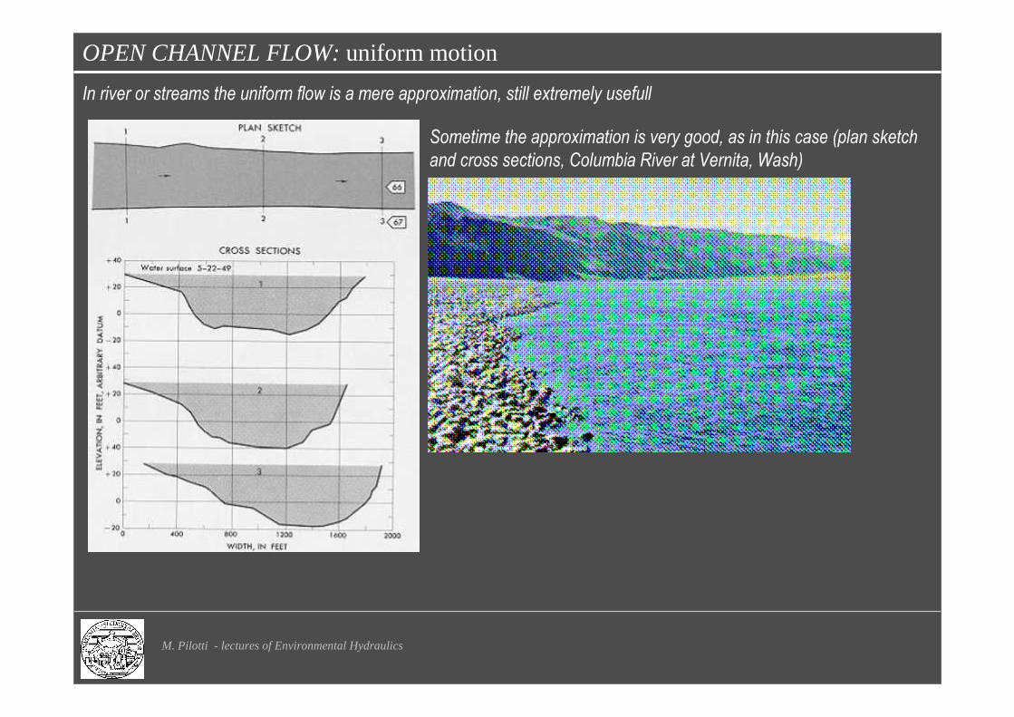
In river or streams the uniform flow is a mere approximation, still extremely usefull
Sometime the approximation is very good, as in this case (plan sketch
and cross sections, Columbia River at Vernita, Wash)
OPEN CHANNEL FLOW: uniform motion
M. Pilotti - lectures of Environmental Hydraulics
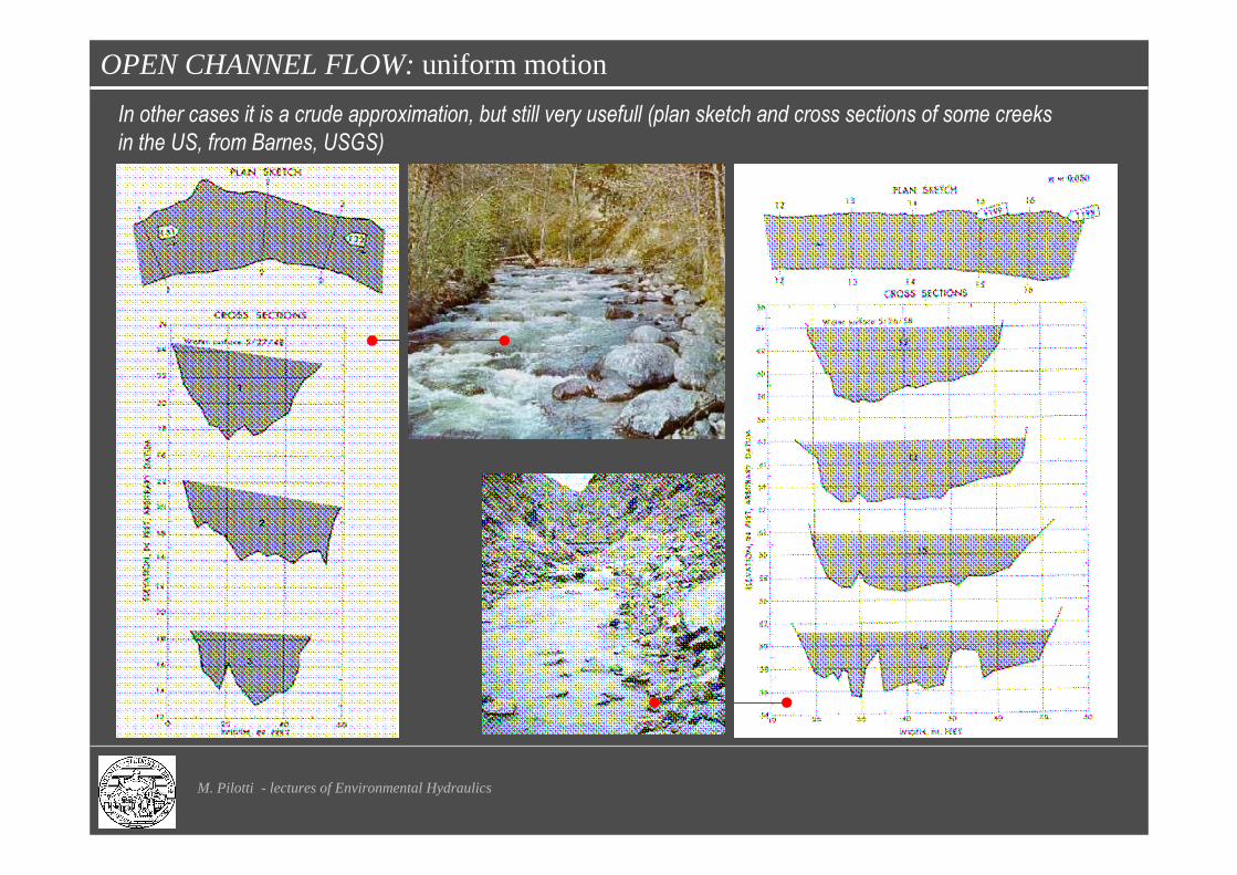
In other cases it is a crude approximation, but still very usefull (plan sketch and cross sections of some creeks
in the US, from Barnes, USGS)

OPEN CHANNEL FLOW: uniform motion
M. Pilotti - lectures of Environmental Hydraulics
bsbs ShP
hAkShRhAhRkQ
3/20
3/50
006/1
0 )(
)()()()( ==
Stage-discharge (scala delle portate) relationship in uniform flow (also, normal rating curve)
The encircled expression is known as conveyance,
being a function of h and representing a measure of
capacity of water transport
h = h0 is the so called
NORMAL DEPTH
(profondità di moto uniforme)
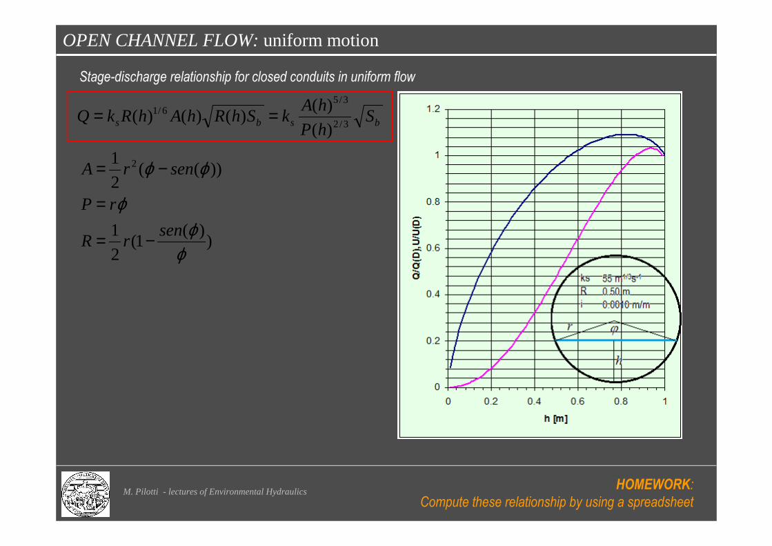
OPEN CHANNEL FLOW: uniform motion
M. Pilotti - lectures of Environmental Hydraulics
bsbs ShP
hAkShRhAhRkQ
3/2
3/56/1
)(
)()()()( ==
Stage-discharge relationship for closed conduits in uniform flow
))(
1(2
1
))((2
1 2
ϕϕ
ϕ
ϕϕ
senrR
rP
senrA
−=
=
−=
HOMEWORK:
Compute these relationship by using a spreadsheet
OPEN CHANNEL FLOW: uniform motion
M. Pilotti - lectures of Environmental Hydraulics
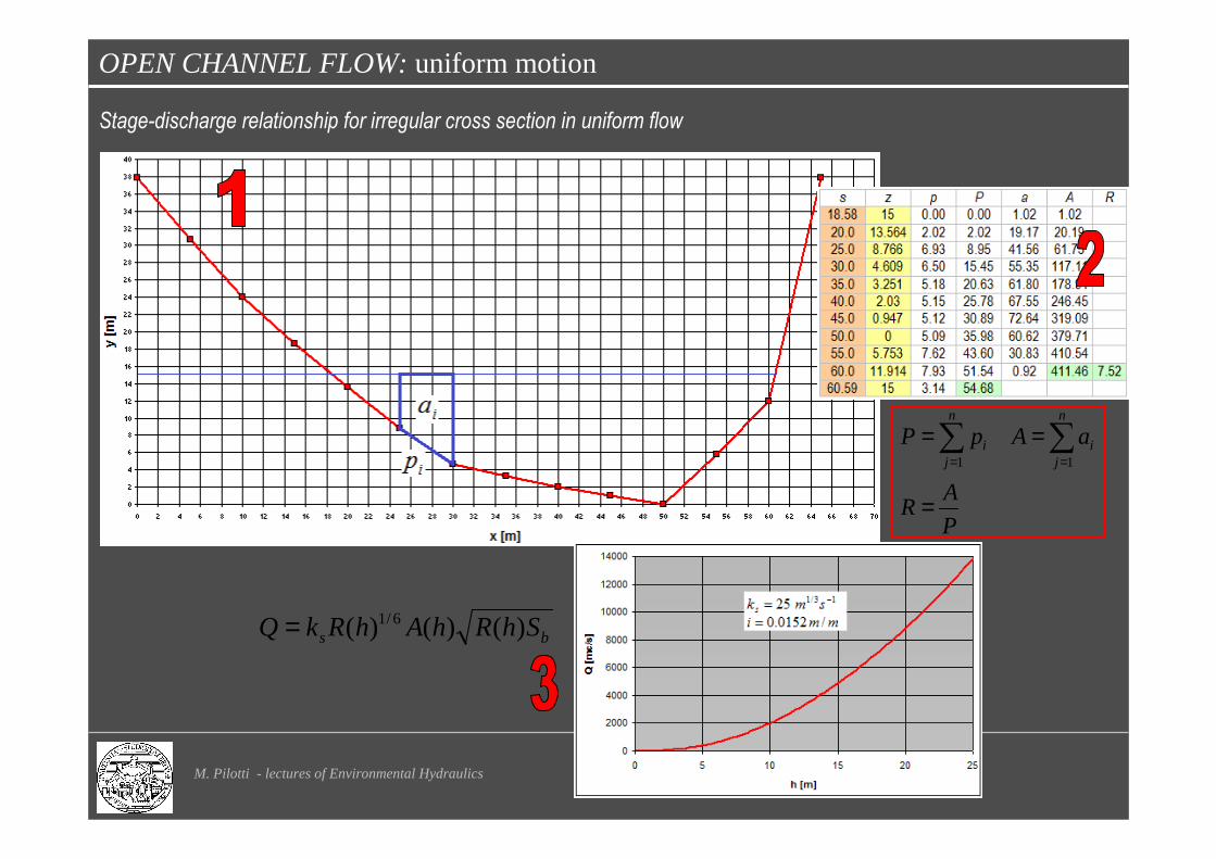
bs ShRhAhRkQ )()()( 6/1=
Stage-discharge relationship for irregular cross section in uniform flow
P
AR
aApPn
ji
n
ji
=
== ∑∑== 11
OPEN CHANNEL FLOW: uniform motion
M. Pilotti - lectures of Environmental Hydraulics
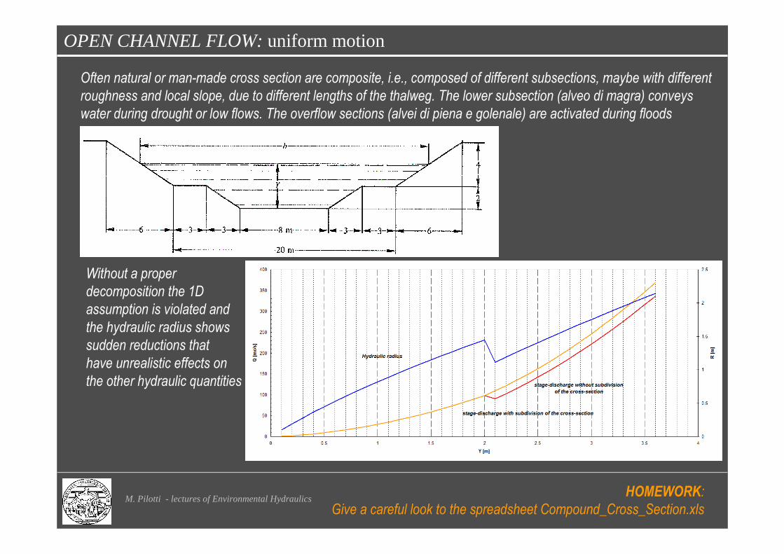
Often natural or man-made cross section are composite, i.e., composed of different subsections, maybe with different
roughness and local slope, due to different lengths of the thalweg. The lower subsection (alveo di magra) conveys
water during drought or low flows. The overflow sections (alvei di piena e golenale) are activated during floods
Without a proper
decomposition the 1D
assumption is violated and
the hydraulic radius shows
sudden reductions that
have unrealistic effects on
the other hydraulic quantities
HOMEWORK:
Give a careful look to the spreadsheet Compound_Cross_Section.xls

OPEN CHANNEL FLOW: uniform motion
M. Pilotti - lectures of Environmental Hydraulics
“Zona golenale” of the Po river at Isola
Pescaroli (floodplain)
“Alveo di magra”
(main bed or
channel)
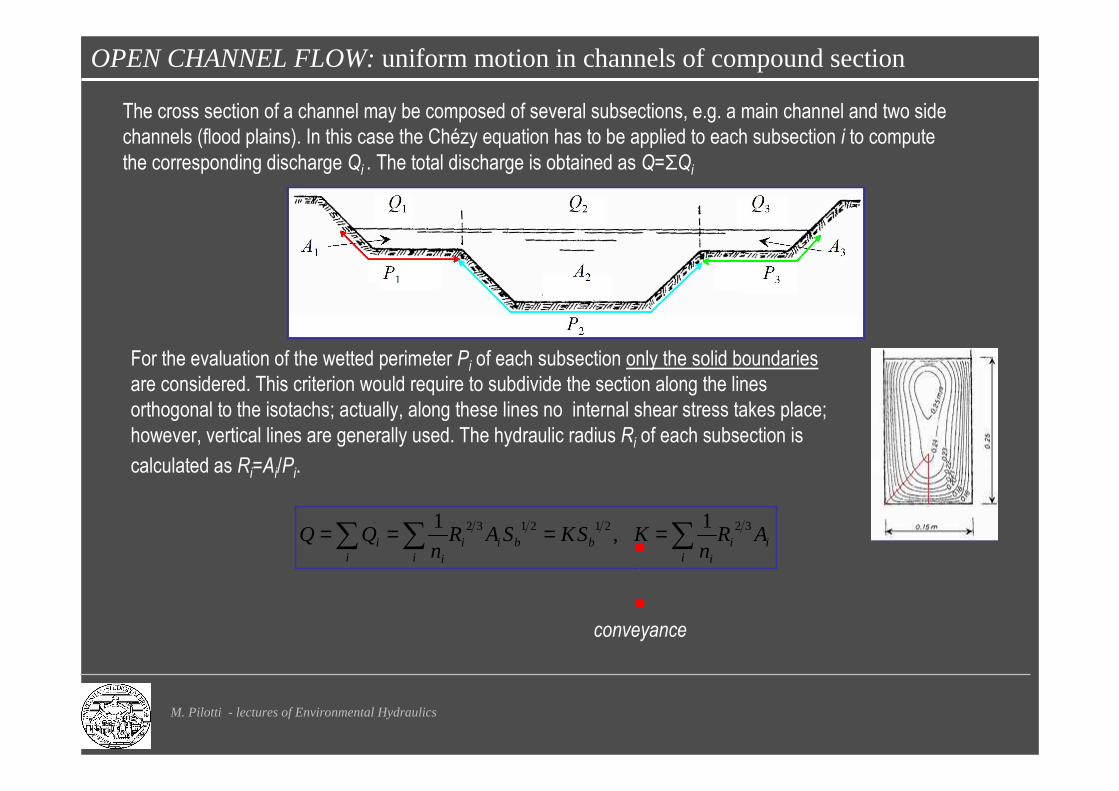
The cross section of a channel may be composed of several subsections, e.g. a main channel and two side
channels (flood plains). In this case the Chézy equation has to be applied to each subsection i to compute
the corresponding discharge Qi . The total discharge is obtained as Q=ΣQi
For the evaluation of the wetted perimeter Pi of each subsection only the solid boundaries
are considered. This criterion would require to subdivide the section along the lines
orthogonal to the isotachs; actually, along these lines no internal shear stress takes place;
however, vertical lines are generally used. The hydraulic radius Ri of each subsection is
calculated as Ri=Ai/Pi.
∑∑∑ ====i
iii
bi
biiii
i ARn
KSKSARn
QQ 32212132 1 ,
1
M. Pilotti - lectures of Environmental Hydraulics
OPEN CHANNEL FLOW: uniform motion in channels of compound section
conveyance

In case of compact sections in which the roughness may be different from part to part of the perimeter the
discharge can be computed without actually subdividing the section. To this purpose, an equivalent roughness
coefficient can be introduced dividing the water area into N parts of which the wetted perimeter Pi (calculated
taking into account only the solid boundaries) and roughness coefficients ni are known.
Assuming the same mean velocity for each partial area, in uniform flow (according to Horton and Einstein)
∑∑
=
= )(
3223
ii
ii
PPP
nPnAnP
P
A
n iii =∑ 23
23
1
from which
⇒
iii
b
i
i
i
ib
b AnPP
A
nS
V
P
A
nP
A
nS
VSR
nV =⇒===⇒= 23
2343
23
232343
232132 1111
M. Pilotti - lectures of Environmental Hydraulics
OPEN CHANNEL FLOW: equivalent roughness
( )3/5
3/5
PR
RkPk isii
s∑=
In a similar way, Pavloskii and
Einstein, considering the tractive force
along the boundary as the sum of the
single contributions
5.0
2
5.0
=
∑si
i
s
k
P
Pk And Lotter, regarding the overall
discharge as the sum of the single
contributions
HOMEWORK:
Compare these relationship by using a spreadsheet
OPEN CHANNEL FLOW: uniform motion
M. Pilotti - lectures of Environmental Hydraulics
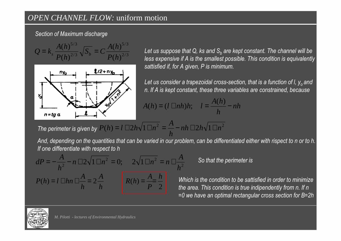
Section of Maximum discharge
3/2
3/5
3/2
3/5
)(
)(
)(
)(
hP
hACS
hP
hAkQ bs == Let us suppose that Q, ks and Sb are kept constant. The channel will be
less expensive if A is the smallest possible. This condition is equivalently
sattisfied if, for A given, P is minimum.
Let us consider a trapezoidal cross-section, that is a function of l, yo and
n. If A is kept constant, these three variables are constrained, because
nhh
hAlhnhlhA −=+= )(
;)()(
The perimeter is given by22 1212)( nhnh
h
AnhlhP ++−=++=
And, depending on the quantities that can be varied in our problem, can be differentiated either with rispect to n or to h.
If one differentiate with respect to h
222
212;012
h
Annnn
h
AdP +=+=++−−= So that the perimeter is
2)(2)(
h
P
AhR
h
A
h
AhnlhP ===++= Which is the condition to be sattisfied in order to minimize
the area. This condition is true indipendently from n. If n
=0 we have an optimal rectangular cross section for B=2h

OPEN CHANNEL FLOW: uniform motion
M. Pilotti - lectures of Environmental Hydraulics
nnn
hnhdP 21;0
1
2 2
2=+=
++−=
Always with A constant, If one can minimize also with
respect to n one obtains this
condition that corresponds to n=tg30°
These two conditions provide an additional constraint to identify the optimal cross section
Accordingly, if everything can be chosen, an half exagonal cross section seems to be the most reasonable.
On the other hand, if the choice is constrained to a rectangular cross-section, B=2h provides the best choice.
Whether this choice is practicable or not depends on other constraints, such as, for instance, the type of lining used to
cover the channel surface, the actual availability of space around the channel or the maximum allowable velocity.
OPEN CHANNEL FLOW: uniform motion and selection of roughness coefficient
M. Pilotti - lectures of Environmental Hydraulics
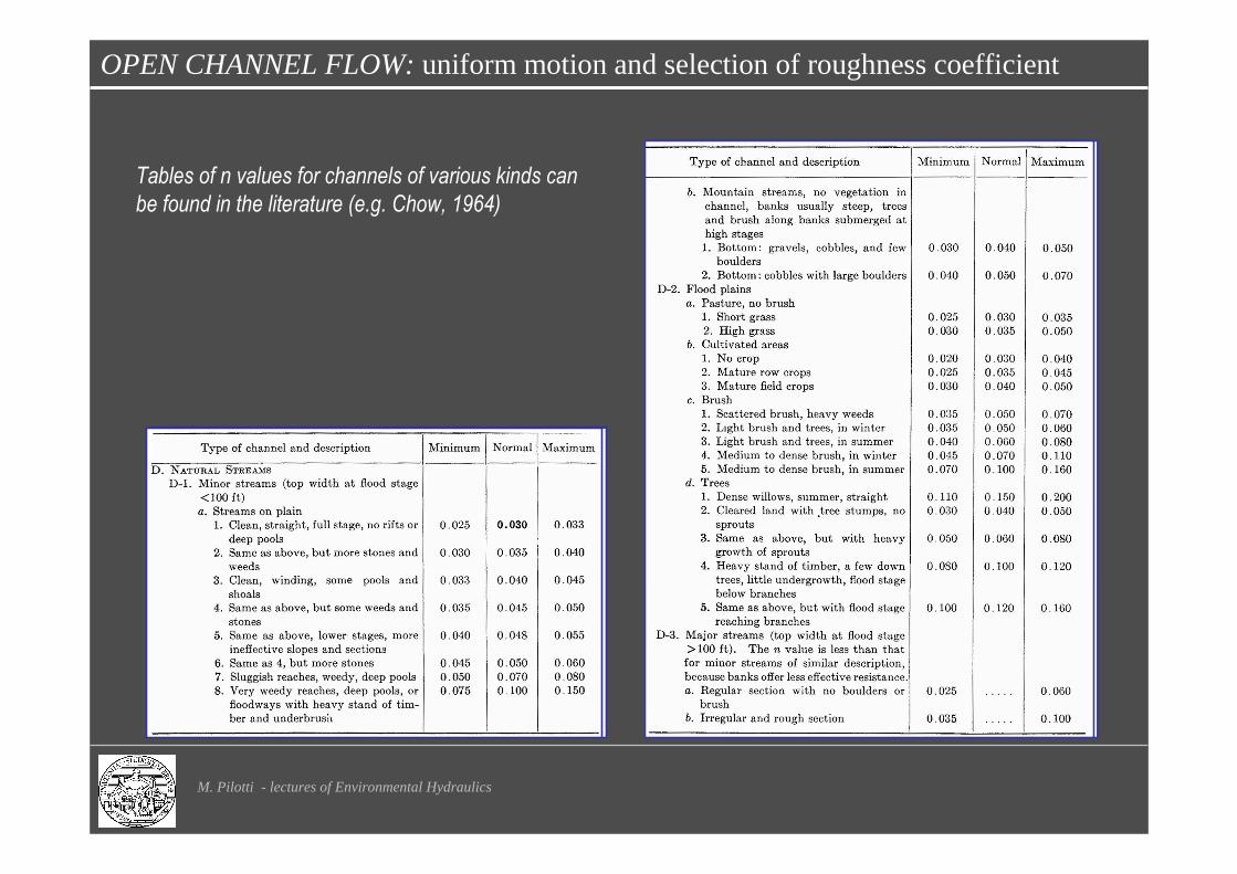
Tables of n values for channels of various kinds can
be found in the literature (e.g. Chow, 1964)

OPEN CHANNEL FLOW: uniform motion and selection of roughness coefficient
M. Pilotti - lectures of Environmental Hydraulics
OPEN CHANNEL FLOW: a remark on the applicability of the fixed bed hypothesis
M. Pilotti - lectures of Environmental Hydraulics
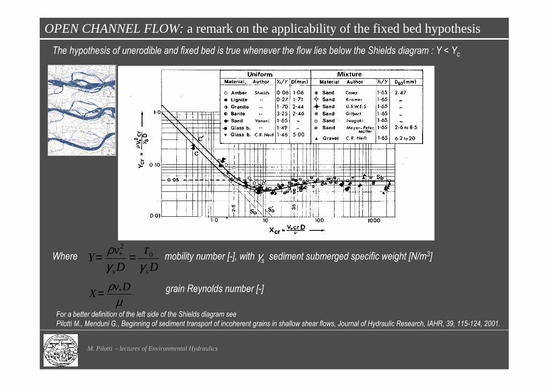
The hypothesis of unerodible and fixed bed is true whenever the flow lies below the Shields diagram : Y < Yc
µρ Dv
X *=
DD
vY
ss γτ
γρ 0
2* ==
grain Reynolds number [-]
Where mobility number [-], with γs sediment submerged specific weight [N/m3]
For a better definition of the left side of the Shields diagram see
Pilotti M., Menduni G., Beginning of sediment transport of incoherent grains in shallow shear flows, Journal of Hydraulic Research, IAHR, 39, 115-124, 2001.
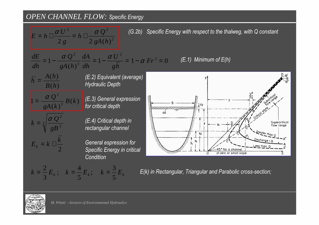
OPEN CHANNEL FLOW: Specific Energy
M. Pilotti - lectures of Environmental Hydraulics
(G.2b) Specific Energy with respect to the thalweg, with Q constant2
22
)(22 hgA
Qh
g
UhE
αα +=+=
kkk
k
EkEkEk
kkE
gB
Qk
kBkgA
Q
hB
hAh
Frhg
U
dh
dA
hgA
Q
dh
dE
5
3;
5
4;
3
2
2
)()(
1
)(
)(
011)(
1
32
2
3
2
22
3
2
===
+=
=
=
=
=−=−=−=
α
α
ααα(E.1) Minimum of E(h)
(E.2) Equivalent (average)
Hydraulic Depth
(E.3) General expression
for critical depth
(E.4) Critical depth in
rectangular channel
General espression for
Specific Energy in critical
Condition
E(k) in Rectangular, Triangular and Parabolic cross-section;

OPEN CHANNEL FLOW: Specific Energy
M. Pilotti - lectures of Environmental Hydraulics
For a given channel
section and a given
discharge the critical
depth yc depends only
on the geometry of the
section, while the
normal depth h = h0
depends on the slope
of the channel and the
roughness coefficient.
Depending on the relative position between h0 and k, the bottom slope is defined as
Mild slope: h0 > k (see figure above); Steep slope: h0 < k; Critical slope: h0 = k

OPEN CHANNEL FLOW: Specific Discharge
M. Pilotti - lectures of Environmental Hydraulics
Specific discharge for E constant( )
( )hEg
hqB
Q
khh
hEdh
dQ
hEg
hAQ
−==
≡→+=→=
−=
α
α
2
20
2)(
In a rectangular cross section

OPEN CHANNEL FLOW: Froude number
M. Pilotti - lectures of Environmental Hydraulics
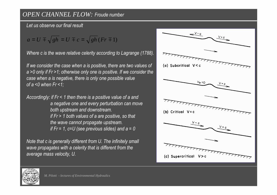
Let us underline the meaning of the Froude number.
Let us consider an infinitely wide channel where water flows in uniform motion
with depth h and velocity U.
If perturbation affects the whole water column (tsunami like), we have a
wave of positive height dh that may travel upstream and downstream with absolute
celerity ±a. Due to its passage U is modified, as U-dU.
Given that the motion is an unsteady one, it is convenient to study the process
as seen from astride the wave. This is a inertial frame of reference so that
both energy and mass balance can be written in terms of relative velocity.
We can write
( ) ( ) ( ) ( )
( ) ( )( ) ( )
)1(
0
220
;22
mmm
rrr
FrghcUghUa
h
aUdhdUdhhadUUhaU
ds
dQ
g
aUdUdh
g
adUUdhh
g
aUh
ds
dE
aUUaUU
vvv
rr
tra
===
−=+−−=−=
−=−−++=−+=
−=+=+=
energy
balance
mass
balance
OPEN CHANNEL FLOW: Froude number
M. Pilotti - lectures of Environmental Hydraulics
Let us observe our final result
)1( mmm FrghcUghUa ===
Where c is the wave relative celerity according to Lagrange (1788).
If we consider the case when a is positive, there are two values of
a >0 only if Fr >1; otherwise only one is positive. If we consider the
case when a is negative, there is only one possible value
of a <0 when Fr <1;
Accordingly: if Fr < 1 then there is a positive value of a and
a negative one and every perturbation can move
both upstream and downstream.
if Fr > 1 both values of a are positive, so that
the wave cannot propagate upstream.
if Fr = 1, c=U (see previous slides) and a = 0
Note that c is generally different from U. The infinitely small
wave propagates with a celerity that is different from the
average mass velocity, U.
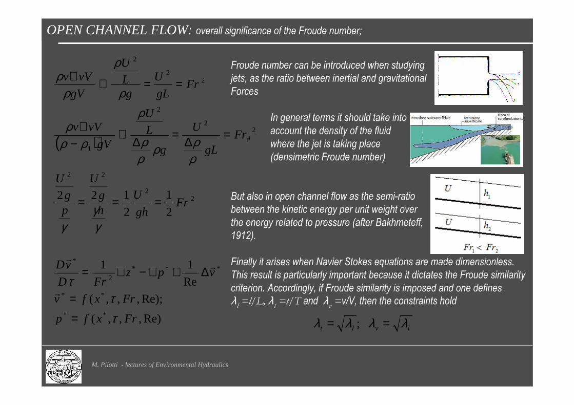
OPEN CHANNEL FLOW: overall significance of the Froude number;
M. Pilotti - lectures of Environmental Hydraulics
( )
Re),,,(
Re);,,,(
Re
11
2
1
2
122
**
**
***2
*
22
22
22
2
1
22
2
Frxfp
Frxfv
vpzFrD
vD
Frgh
Uhg
U
pg
U
FrgL
U
g
L
U
gV
vVv
FrgL
U
gL
U
gV
vVv
d
ττ
τ
γγ
γ
ρρρ
ρρ
ρ
ρρρ
ρ
ρ
ρρ
==
∆+∇−∇=
===
=∆=∆∝−
∇
==∝∇
r
rr
Froude number can be introduced when studying
jets, as the ratio between inertial and gravitational
Forces
In general terms it should take into
account the density of the fluid
where the jet is taking place
(densimetric Froude number)
But also in open channel flow as the semi-ratio
between the kinetic energy per unit weight over
the energy related to pressure (after Bakhmeteff,
1912).
Finally it arises when Navier Stokes equations are made dimensionless.
This result is particularly important because it dictates the Froude similarity
criterion. Accordingly, if Froude similarity is imposed and one defines
λl=l/L, λ
t=t/T and λ
v=v/V, then the constraints hold
lvlt λλλλ == ;

OPEN CHANNEL FLOW: steady flow profiles in prismatic channels
M. Pilotti - lectures of Environmental Hydraulics
Let us consider a gradually varied flow, i.e. one in which vertical acceleration on the cross section are negligeable,
and, accordingly, an hydrostatic pressure distribution is present. This happens if the slope of the channel is small
and the geometry of the boundary is such that the streamlines are practically parallel. Under the above hypotheses,
starting from energy equation of gradually varied flow.
dx
dA
A
E
dx
dy
y
ES
gA
Qyz
dx
d
dx
dH
∂∂+
∂∂+−=
++= 02
2
2
fSdx
dH −=
23
2
2
2
112
, FrgA
bQ
gA
Qy
dy
d
dy
dE
dydE
SS
dx
dy fb −=−=
+=
−=
2
20
2
20
22
1
1
1
)(1
Fr
QQS
Fr
SKQS
dx
dybb −
−=−
−=
Let us now consider a prismatic channels, so that
A=A(y(x)) and Sb=constant

OPEN CHANNEL FLOW: steady flow profiles in prismatic channels
M. Pilotti - lectures of Environmental Hydraulics
From the equation of gradually varied flow in a prismatic channel, the following general properties of the flow profile
y(x) are easily obtained:
.
(asymptotic to a horizontal line)
220
2
1,1,);(
);(FrD
Q
QSN
QyD
QyN
dx
dyb −=
−==
bSdx
dy
D
N
Fr
Qy →⇒
→→
⇒
→∞→
⇒∞→ 1
1
0 0
0 0
−∞→−∞→
⇒
∞→∞→
⇒→D
N
Fr
Qy
00
0 00 →⇒
≠→
⇒→⇒→dx
dy
D
NQQyy
∞→⇒
→≠
⇒→⇒→dx
dy
D
NFryy c
0
0 1
(asymptotic to normal-depth line)
(asymptotic to a vertical line)
(dy/dx→ ∞ if Manning eq. Is used for Q0)
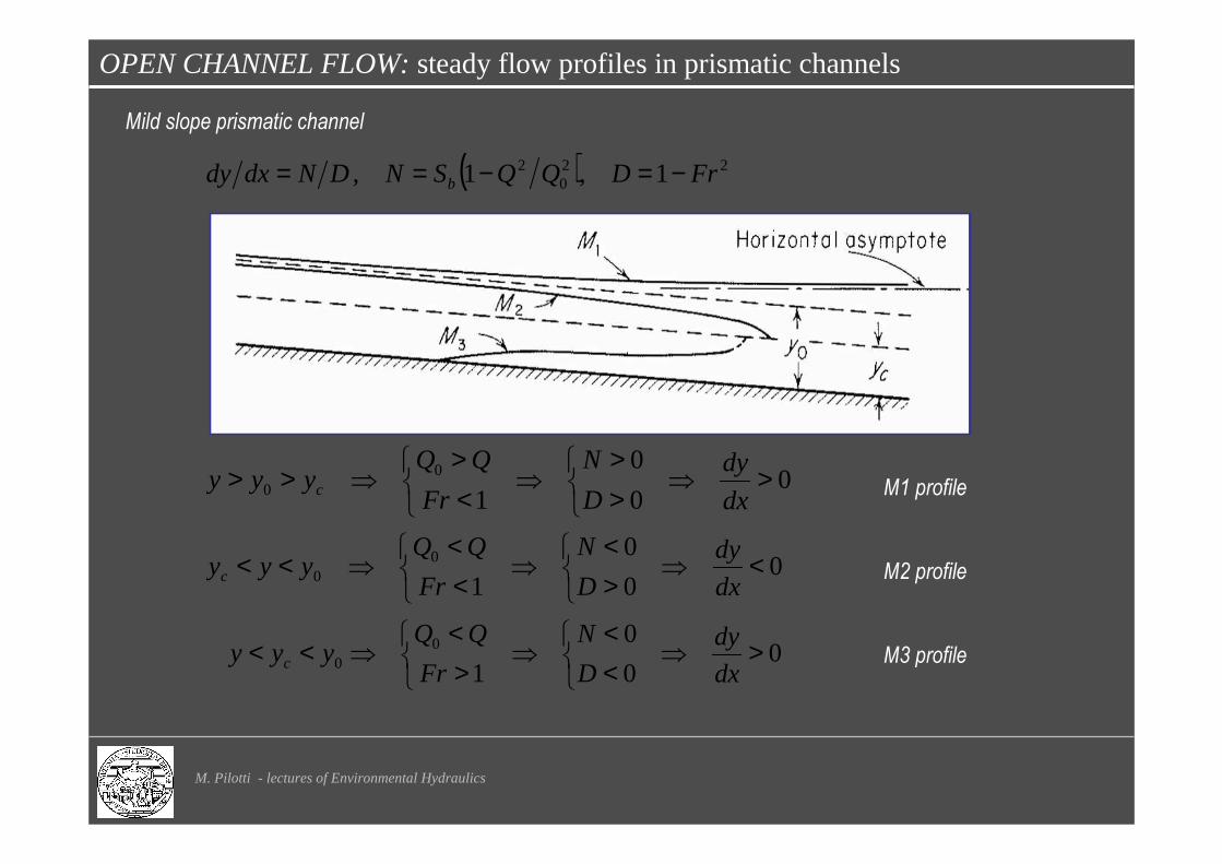
OPEN CHANNEL FLOW: steady flow profiles in prismatic channels
M. Pilotti - lectures of Environmental Hydraulics
00
0
10
0 >⇒
>>
⇒
<>
⇒>>dx
dy
D
N
Fr
QQyyy c
00
0
10
0 <⇒
><
⇒
<<
⇒<<dx
dy
D
N
Fr
QQyyyc
00
0
10
0 >⇒
<<
⇒
><
⇒<<dx
dy
D
N
Fr
QQyyy c
( ) 220
2 1,1, FrDQQSNDNdxdy b −=−==
Mild slope prismatic channel
M1 profile
M2 profile
M3 profile

OPEN CHANNEL FLOW: steady flow profiles in mild slope prismatic channels
M. Pilotti - lectures of Environmental Hydraulics
From W. H. Graf and
M. S. Altinakar, 1998

OPEN CHANNEL FLOW: steady flow profiles in prismatic channels
M. Pilotti - lectures of Environmental Hydraulics
Steep slope prismatic channel
S1 profile
S2 profile
S3 profile
00
0
10
0 >⇒
>>
⇒
<>
⇒>>dx
dy
D
N
Fr
QQyyy c
00
0
10
0 >⇒
<<
⇒
><
⇒<<dx
dy
D
N
Fr
QQyyy c
00
0
10
0 <⇒
<>
⇒
>>
⇒<<dx
dy
D
N
Fr
QQyyy c
( ) 220
20 1,1, FrDQQSNDNdxdy −=−==
OPEN CHANNEL FLOW: steady flow profiles in steep slope prismatic channels
M. Pilotti - lectures of Environmental Hydraulics
Boundary conditions:
Q known;
If Fr<1, Y downstream and the
computation proceeds in the
upstream direction along the
channel.
If Fr>1, Y upstream and the
computation proceeds in the
downstream direction along the
channel.
From W. H. Graf and M. S. Altinakar, 1998

OPEN CHANNEL FLOW: steady flow profiles in prismatic channels
M. Pilotti - lectures of Environmental Hydraulics
Horizontal slope prismatic channel
Adverse slope prismatic channel
Critical slope prismatic channel
OPEN CHANNEL FLOW: steady flow profiles in various slope prismatic channels
M. Pilotti - lectures of Environmental Hydraulics
From W. H. Graf and M. S. Altinakar, 1998
Horizontal slope prismatic channel
Adverse slope prismatic channel
Critical slope prismatic channel
OPEN CHANNEL FLOW: hydraulic jump
M. Pilotti - lectures of Environmental Hydraulics
Supercritical flow in mild slope prismatic channels (M3 profile) and subcritical flow in steep slope prismatic channels
(S1 profile) are limited downstream and upstream respectively at the critical depth. In these cases it may happen that
supercritical flow has to be followed by subcritical flow to cover the whole channel length.
The change from supercritical to subcritical flow takes place abruptly through a vortex known as the hydraulic jump,
characterized by considerable turbulence and energy loss.
The flow depths upstream and downsteam of the jump are called sequent depths or conjugate depths.
OPEN CHANNEL FLOW: hydraulic jump
M. Pilotti - lectures of Environmental Hydraulics
OPEN CHANNEL FLOW: hydraulic jump
M. Pilotti - lectures of Environmental Hydraulics
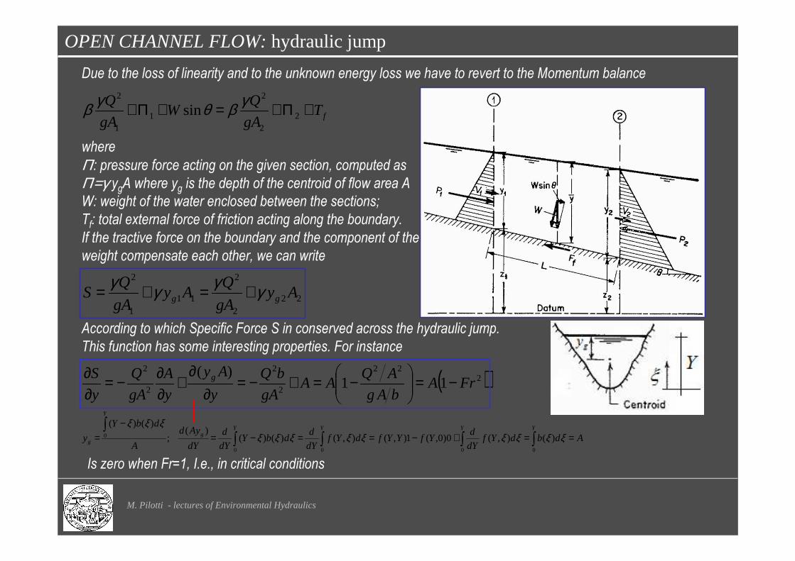
Due to the loss of linearity and to the unknown energy loss we have to revert to the Momentum balance
where
Π: pressure force acting on the given section, computed as
Π=γ ygA where yg is the depth of the centroid of flow area A
W: weight of the water enclosed between the sections;
Tf: total external force of friction acting along the boundary.
If the tractive force on the boundary and the component of the
weight compensate each other, we can write
According to which Specific Force S in conserved across the hydraulic jump.
This function has some interesting properties. For instance
fTgA
QW
gA
Q +Π+=+Π+ 22
2
11
2
sinγβθγβ
222
2
111
2
AygA
QAy
gA
QS gg γγγγ +=+=
( )222
2
2
2
2
11)(
FrAbAg
AQAA
gA
bQ
y
Ay
y
A
gA
Q
y
S g −=
−=+−=
∂∂
+∂∂−=
∂∂
Is zero when Fr=1, I.e., in critical conditions
∫∫∫∫∫
==+−==−=−
=YYYY
g
Y
g AdbdYfdY
dYfYYfdYf
dY
ddbY
dY
d
dY
Ayd
A
dbY
y0000
0 )(),(0)0,(1),(),()()()(
;
)()(
ξξξξξξξξξξξξ

OPEN CHANNEL FLOW: hydraulic jump
M. Pilotti - lectures of Environmental Hydraulics
From the momentum
equation
in the form S1=S2 it turn out
that since E2<E1 an energy
loss ∆E=E2-E1 takes place
across the jump
y1 is the initial depth (depth
before the jump) and y2 the
sequent depth.
Both are coniugate depths
OPEN CHANNEL FLOW: hydraulic jump
M. Pilotti - lectures of Environmental Hydraulics
For rectangular sections the condition of momentum conservation between sections 1 and 2 can be written as
Whose solution, due to the symmetry of the equation, can be put in one of the followig forms that can be used to
calculate downstream (or upstream) depth once upstream (or downstream) conditions are known:
The energy loss across the jump can be calculated as:
Experimental investigations show that in the range ?<Fr1<? the length of the jump is L ≅ 6y2??
( )18121 2
11
2 −+= Fry
y ( )18121 2
22
1 −+= Fry
y
21
312
22
2
2
221
2
2
121 4)(
22 yy
yy
ybg
Qy
ybg
QyEE
−=−−+=−
2
2
2121
22
2
221
1
2 2)(
22 bg
Qyyyy
yb
ybg
Qyb
ybg
Q =+⇒+=+
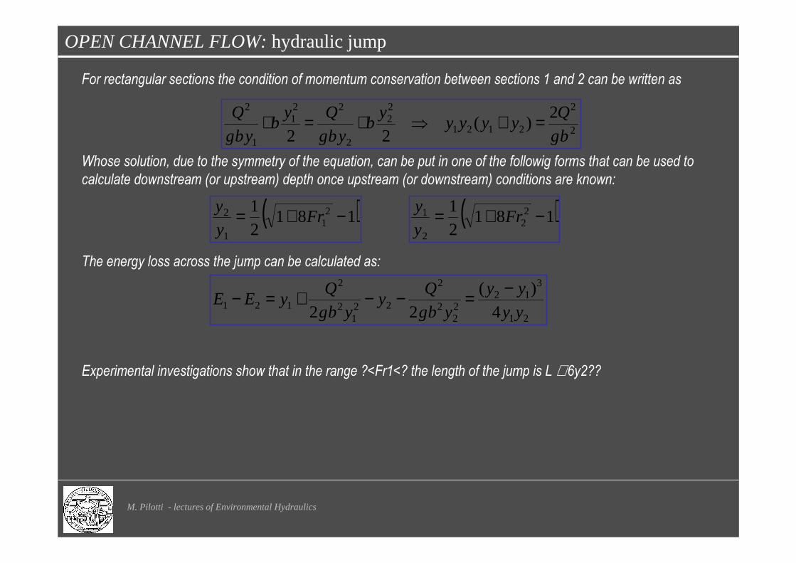
OPEN CHANNEL FLOW: qualitative profiles in complex channels
M. Pilotti - lectures of Environmental Hydraulics
Real cases can be obtained by combining the simple
profiles seen before.
As a first step control section must be identified, where
the depth is known as a function of Q. From there one
starts computing the profile moving in the direction
dictated by the Froude number, as far as the critical
depth is reached.
At this stage, in some stretch of the channel, more than
a single profile is potentially present. The final choice
will be the one whose Specific Force prevails.

OPEN CHANNEL FLOW: quantitative profiles in complex channels
M. Pilotti - lectures of Environmental Hydraulics
Initially, in order to understand what is the actual applicability scope of uniform motion we asked how much
far away is far ? When an M1 profile is considered a first guess can be provided by the following table, that is
valid for infinitely wide rectangular channel, according to Bresse’s solution
OPEN CHANNEL FLOW: quantitative profiles in complex channels
M. Pilotti - lectures of Environmental Hydraulics
Direct step method
(distance calculated from depth)
fb SSdx
dE −=
y1 at the position x1 along the channel is known as a boundary condition. From the qualitative discussion of
the profile, one knows what is the asymptotic depth (e.g., if M1, it will tend to h0). Accordingly one selects in an
adaptive way a depth value y1 < yi+1 < h0 for the section at the unknown station xi+1, computing the
corresponding values Ei+1 and (Sf)i+1 (that depend only on yi+1 in prismatic channels). The unknown station xi+1
is obtained by discretization of the dynamic equation
[ ]10
11
)()(21
+
++
+−
−+=ifif
iiii
SSS
EExx⇒[ ] )()()(
21
)( 11101 iiififiiii xxSSxxSEE −+−−=− ++++
Let us first consider a method which is very convenient but is valid only in prismatic channel, where,
indeipendently from x, one knows A(x) and Sb(x)
OPEN CHANNEL FLOW: quantitative profiles in complex channels
M. Pilotti - lectures of Environmental Hydraulics
Standard step method
(depth calculated from distance)
Let us now consider a general method which can be as convenient as the direct step if solved explicitly or just
a bit more complex if solved implicitly. Its scope is not limited to prismatic channels.
We know the boundary condition yi at the position xi along the channel. By a first order approximation of the
energy balance equation, we obtain :
The unknown value yi+1 at the position xi+1 is such that F=0
This equation is non linear and must be solved by, e.g., a Newton Raphson method.
As a first guess for the iteration, a first estimate y*i+1 of yi+1 can be obtained as
that can also be used as an explicit approximation of the energy balance equation
fSdx
dH −= [ ] )()()(21
111 iiififii xxSSHH −+−=− +++⇒
)()( 1*
1*
1*
1 ++++ ′−= iiii yFyFyy
2/)]()()[()( where,0)( 11111 iiififiiii xxSSHHyFyF −++−== +++++
)()()(2 12
1
2
11 iiifiii
ii xxSHygA
Qzy −−+−−= +
+++ α
IMPLICIT
EXPLICIT
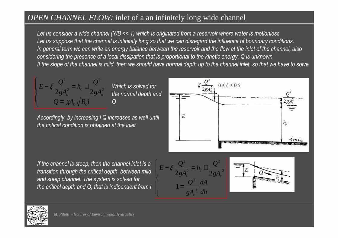
OPEN CHANNEL FLOW: inlet of a an infinitely long wide channel
M. Pilotti - lectures of Environmental Hydraulics
Let us consider a wide channel (Y/B << 1) which is originated from a reservoir where water is motionless
Let us suppose that the channel is infinitely long so that we can disregard the influence of boundary conditions.
In general term we can write an energy balance between the reservoir and the flow at the inlet of the channel, also
considering the presence of a local dissipation that is proportional to the kinetic energy. Q is unknown
If the slope of the channel is mild, then we should have normal depth up to the channel inlet, so that we have to solve
=
+=−
iRAQ
gA
Qh
gA
QE
oo
oo
o
χ
ξ2
2
2
2
22
Accordingly, by increasing i Q increases as well until
the critical condition is obtained at the inlet
If the channel is steep, then the channel inlet is a
transition through the critical depth between mild
and steep channel. The system is solved for
the critical depth and Q, that is indipendent from i
=
+=−
dh
dA
gA
QgA
Qh
gA
QE
c
c
cc
3
2
2
2
2
2
1
22ξ
Which is solved for
the normal depth and
Q

OPEN CHANNEL FLOW: inlet of a short and wide channel - mild slope case
M. Pilotti - lectures of Environmental Hydraulics
If the channel is not infinitely long, then we may have a backwater (rigurgito) or drawdown (chiamata) effect caused
by the boundary condition located at the channel outlet. In this case the discharge is computed through an iterative
procedure.
Let us suppose that the channel outlet is into another reservoir, that conditions the level of water at the channel
end, he If the channel is mild, the discharge computed from the system seen before is only an initial guess
1) From Q, compute the critical depth hc
2) If he < hc compute a M2 profile starting from hc, otherwise either a M2 profile (hc <he < ho ) or an M1 one (he > ho )
3) Compare the computed water depth at the channel sill (inlet) with the normal depth. If it is higher, than Q must be
decreased; otherwise it must be increased.
If he = E +il, then Q = 0;
If he > E +il, the flow is reversed from downstream to upstream. The mild slope channel turns into an adverse slope one
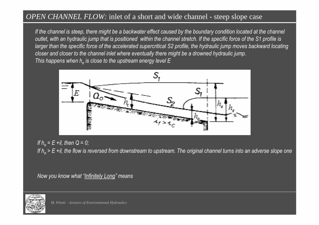
OPEN CHANNEL FLOW: inlet of a short and wide channel - steep slope case
M. Pilotti - lectures of Environmental Hydraulics
If the channel is steep, there might be a backwater effect caused by the boundary condition located at the channel
outlet, with an hydraulic jump that is positioned within the channel stretch. If the specific force of the S1 profile is
larger than the specific force of the accelerated supercritical S2 profile, the hydraulic jump moves backward locating
closer and closer to the channel inlet where eventually there might be a drowned hydraulic jump.
This happens when he is close to the upstream energy level E
If he = E +il, then Q = 0;
If he > E +il, the flow is reversed from downstream to upstream. The original channel turns into an adverse slope one
Now you know what “Infinitely Long” means
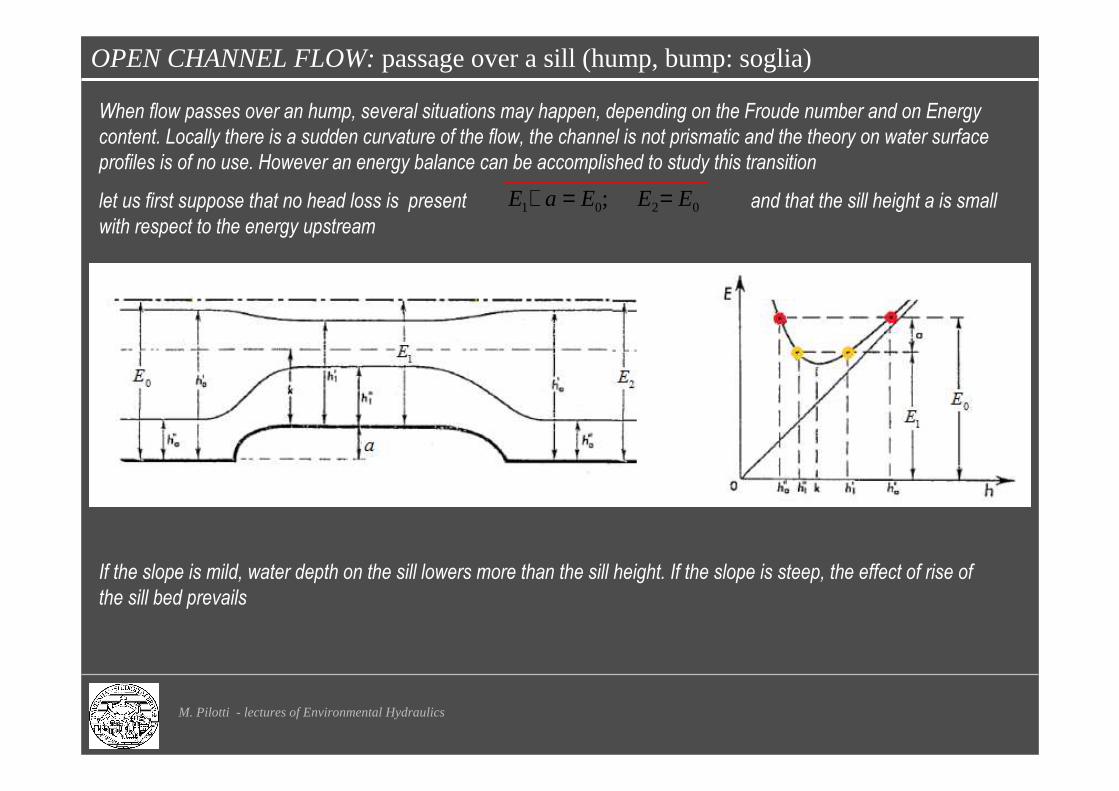
OPEN CHANNEL FLOW: passage over a sill (hump, bump: soglia)
M. Pilotti - lectures of Environmental Hydraulics
When flow passes over an hump, several situations may happen, depending on the Froude number and on Energy
content. Locally there is a sudden curvature of the flow, the channel is not prismatic and the theory on water surface
profiles is of no use. However an energy balance can be accomplished to study this transition
let us first suppose that no head loss is present and that the sill height a is small
with respect to the energy upstream
If the slope is mild, water depth on the sill lowers more than the sill height. If the slope is steep, the effect of rise of
the sill bed prevails
0201 ; EEEaE ==+

OPEN CHANNEL FLOW: passage over a sill (hump, bump: soglia)
M. Pilotti - lectures of Environmental Hydraulics
Sometimes the height of the sill is such that the specific energy in normal flow is not sufficient to pass over it.
Again, we have to distinguish between mild and steep channel
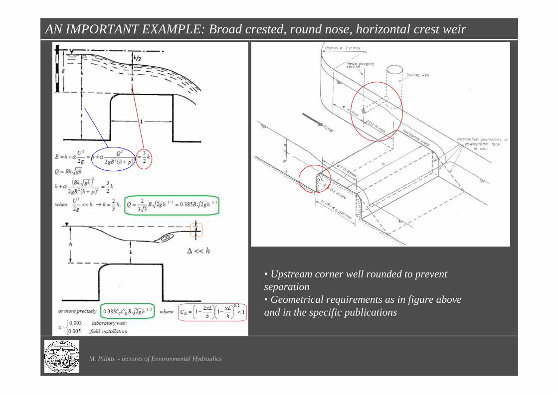
AN IMPORTANT EXAMPLE: Broad crested, round nose, horizontal crest weir
• Upstream corner well rounded to prevent separation• Geometrical requirements as in figure above and in the specific publications
M. Pilotti - lectures of Environmental Hydraulics
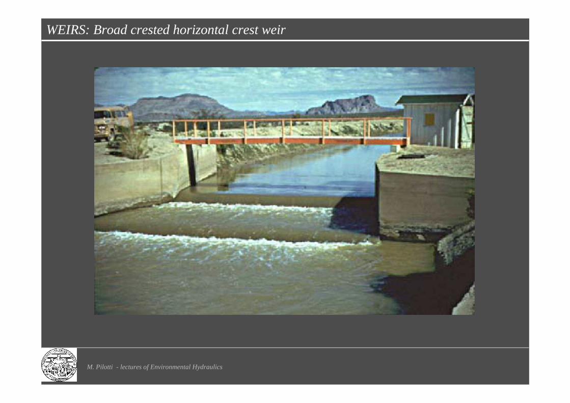
WEIRS: Broad crested horizontal crest weir
M. Pilotti - lectures of Environmental Hydraulics
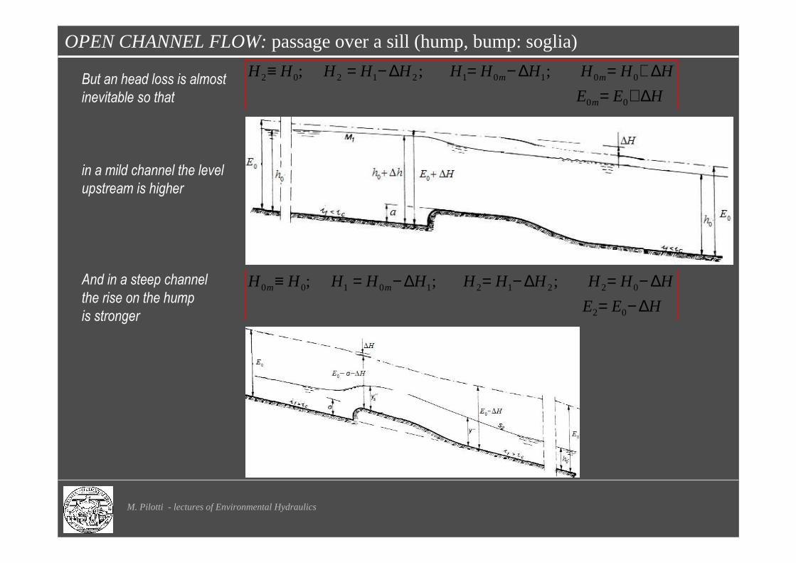
OPEN CHANNEL FLOW: passage over a sill (hump, bump: soglia)
M. Pilotti - lectures of Environmental Hydraulics
But an head loss is almost
inevitable so that
in a mild channel the level
upstream is higher
And in a steep channel
the rise on the hump
is stronger
HEE
HHHHHHHHHHH
m
mm
∆+=∆+=∆−=∆−=≡
00
0010121202 ;;;
HEE
HHHHHHHHHHH mm
∆−=∆−=∆−=∆−=≡
02
0221210100 ;;;
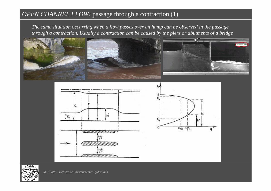
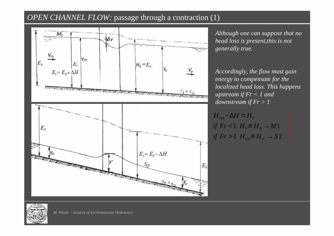
OPEN CHANNEL FLOW: passage through a contraction (1)
M. Pilotti - lectures of Environmental Hydraulics
The same situation occurring when a flow passes over an hump can be observed in the passage through a contraction. Usually a contraction can be caused by the piers or abutments of a bridge
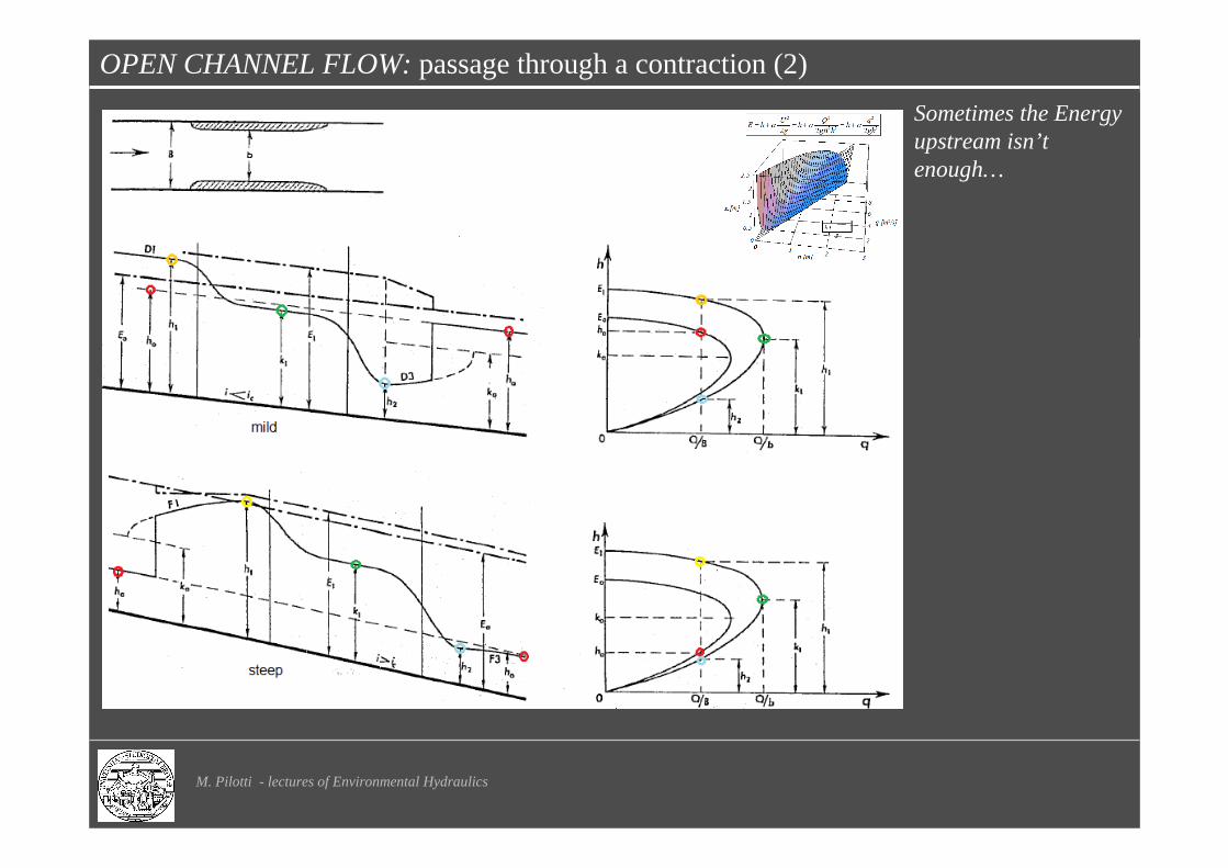
OPEN CHANNEL FLOW: passage through a contraction (2)
M. Pilotti - lectures of Environmental Hydraulics
Sometimes the Energy upstream isn’t enough…
OPEN CHANNEL FLOW: passage through a contraction (1)
M. Pilotti - lectures of Environmental Hydraulics
Although one can suppose that no head loss is present,this is not generally true.
Accordingly, the flow must gain energy to compensate for the localized head loss. This happens upstream if Fr < 1 and downstream if Fr > 1
21
11
00
0
0
SHHFrif
MHHFrif
HHH
m
V
Vm
→≡>→≡<
=∆−

OPEN CHANNEL FLOW: Transitions in subcritical flow
M. Pilotti - lectures of Environmental Hydraulics
Let us consider an abrupt drop in the channel floor. If we have an head loss we cannot directly use an energy balance and we have to revert to a momentum balance, under the same assumptions usually used to derive Borda’s head loss in a pipe.
22
)(
)(
22
2
221
1
2
22
2
11
2
bh
gbh
Qahb
ahgb
Q
gA
Q
gA
Q
γγγγ
γβγβ
+=+++
Π+=Π+
HgA
Qha
gA
QhHEaE
HHH
∆++=++∆+=+
∆+=
22
2
221
2
121
21
22;
If we now consider an energy balance
we get under reasonable assumptions (e.g., Ghetti, pag 395)
( )g
UUH
2
221 −=∆

OPEN CHANNEL FLOW: Transitions
M. Pilotti - lectures of Environmental Hydraulics
As a first approximation one can disregard the energy losses implied in a transition. In such a case the following situations arise for a sudden rise/fall of the bed or contraction/expansion
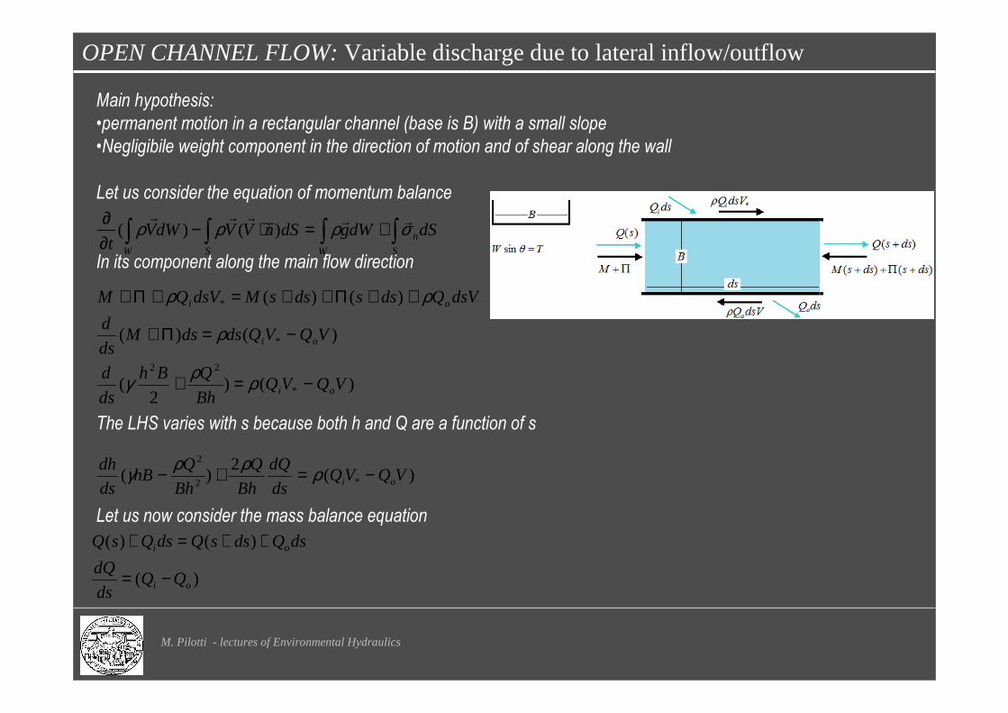
OPEN CHANNEL FLOW: Variable discharge due to lateral inflow/outflow
M. Pilotti - lectures of Environmental Hydraulics
Main hypothesis:
•permanent motion in a rectangular channel (base is B) with a small slope
•Negligibile weight component in the direction of motion and of shear along the wall
Let us consider the equation of momentum balance
In its component along the main flow direction
The LHS varies with s because both h and Q are a function of s
Let us now consider the mass balance equation
∫∫∫∫ +=⋅−∂∂
S
n
WSW
dSdWgdSnVVdWVt
σρρρ rrrrrr)()(
)()2
(
)()(
)()(
*
22
*
*
VQVQBh
QBh
ds
d
VQVQdsdsMds
d
dsVQdssdssMdsVQM
oi
oi
oi
−=+
−=Π+
++Π++=+Π+
ρργ
ρ
ρρ
)(2
)( *2
2
VQVQds
dQ
Bh
Q
Bh
QhB
ds
dhoi −=+− ρρργ
)(
)()(
oi
oi
QQds
dQ
dsQdssQdsQsQ
−=
++=+

OPEN CHANNEL FLOW: lateral outflow - Q decreasing along the flow direction
M. Pilotti - lectures of Environmental Hydraulics
Case A: Qi=0; discharge decreasing along the flow direction
Which can be combined to obtain
If we now consider the flow specific energy E
It varies with s as a function of h and Q
o
o
Qds
dQ
VQds
dQ
Bh
Q
Bh
QhB
ds
dh
−=
−=+− ρρργ 2)(
2
2
0)()2
()( 2
2
2
2
=+−=−+−ds
dQ
Bh
Q
Bh
QhB
ds
dhV
Bh
Q
ds
dQ
Bh
QhB
ds
dh ρργρρργ
22
2
2 hgB
QhE +=
22
32
2
1
hgB
Q
Q
E
hgB
Q
h
E
ds
dQ
Q
E
ds
dh
h
E
ds
dE
=∂∂
−=∂∂
∂∂+
∂∂=
OPEN CHANNEL FLOW: lateral outflow - Q decreasing along the flow direction
M. Pilotti - lectures of Environmental Hydraulics
If one consider that
The momentum balance equation can be written as
or, more simply
And alternatively
Both equations require an additional equation for water overflowing out of the channel. Usually it is in the form
Although an analytical solution is possible if µ is constant, a numerical solution provides a more general approach
Bh
Q
Q
EhB
Bh
QhB
h
EhB
ργ
ργγ
=∂∂
−=∂∂
2
2
0=∂∂+
∂∂
ds
dQ
Q
EhB
ds
dh
h
EhB γγ
0=ds
dE
ds
dQ
h
Q
Q
Bghds
dh
)(
122
−−=
water overflow from the channel happens without decreasing the energy per unit
weight of the water flowing in the channel. Its value will be determined on the
basis of the boundary condition
In an alternative way this equation provides the water surface profile differential
equation. It can be integrated numerically.
( ) 2/32 chgQds
dQo −=−= µ

OPEN CHANNEL FLOW: lateral outflow - Q decreasing along the flow direction
M. Pilotti - lectures of Environmental Hydraulics
E constant and Q decreasing along the flow: use of the Specific discharge curve
Two different classes of problem:
(1) L and c are given; find out Qods, i.e., Q(L) - CONTROL problem
If Fr < 1, starts downstream (station A) with a temptative Q(L) and a corresponding hi(Q(L) ) and compute profile in a
backward fashion. Change Q(L) until Q(0) is found. If Fr > 1, starts upstream (B) knowing hi and Q(0) and compute Q(L).
(2) Qods is given; find out L or c - DESIGN problem
If Fr < 1, starts downstream (station A) with the known value Q(L),hi and compute profile in a backward fashion. When
Q(s)= Q(0), then L = s. If Fr > 1, starts upstream (B) with the known value Q(s),hi and compute profile until
Q(s)=Q(0) - Qods. then L = s.
( )hEg
hqB
Q −==α2