Open Archive TOULOUSE Archive Ouverte (OATAO) · Ces modèles ont été calibrés sur la première moitié de la pé- riode 1988–2005en utilisant les données de température supérieures

This is an author-deposited version published in : http://oatao.univ-toulouse.fr/

Eprints ID : 4891

To link to this article: DOI: 10.1051/kmae/2010031

URL: http://dx.doi.org/10.1051/kmae/2010031

Open Archive TOULOUSE Archive Ouverte (OATAO)OATAO is an open access repository that collects the work of Toulouse researchers and

makes it freely available over the web where possible.

To cite this version : Larnier, K. and Roux, H. and Dartus, D. and

Croze, O. Water temperature modeling in the Garonne River

(France). (2010) Knowledge and Management of Aquatic

Ecosystems, vol. 398 (n° 4). ISSN 1961-9502

Knowledge and Management of Aquatic Ecosystems (2010) 398, 04 http://www.kmae-journal.orgc© ONEMA, 2010

DOI: 10.1051/kmae/2010031

Water temperature modeling in the Garonne River(France)

K. Larnier(1,2), H. Roux(1,2), D. Dartus(1,2), O. Croze(1,2,3)

Received May 4, 2010 / Reçu le 4 mai 2010

Revised July 17, 2010 / Révisé le 17 juillet 2010

Accepted July 29, 2010 / Accepté le 29 juillet 2010

ABSTRACT

Key-words:watertemperature,model,statistical,equilibriumconcept,stochastic,migrating fishes

Stream water temperature is one of the most important parameters forwater quality and ecosystem studies. Temperature can influence manychemical and biological processes and therefore impacts on the livingconditions and distribution of aquatic ecosystems. Simplified models suchas statistical models can be very useful for practitioners and water re-source management. The present study assessed two statistical mod-els – an equilibrium-based model and stochastic autoregressive modelwith exogenous inputs – in modeling daily mean water temperatures inthe Garonne River from 1988 to 2005. The equilibrium temperature-basedmodel is an approach where net heat flux at the water surface is ex-pressed as a simpler form than in traditional deterministic models. Thestochastic autoregressive model with exogenous inputs consists of de-composing the water temperature time series into a seasonal componentand a short-term component (residual component). The seasonal com-ponent was modeled by Fourier series and residuals by a second-orderautoregressive process (Markov chain) with use of short-term air temper-atures as exogenous input. The models were calibrated using data of thefirst half of the period 1988–2005 and validated on the second half. Cali-bration of the models was done using temperatures above 20 ◦C only toensure better prediction of high temperatures that are currently at stake forthe aquatic conditions of the Garonne River, and particularly for freshwa-ter migrating fishes such as Atlantic Salmon (Salmo salar L.). The resultsobtained for both approaches indicated that both models performed wellwith an average root mean square error for observed temperatures above20 ◦C that varied on an annual basis from 0.55 ◦C to 1.72 ◦C on valida-tion, and good predictions of temporal occurrences and durations of threetemperature threshold crossings linked to the conditions of migration andsurvival of Atlantic Salmon.

RÉSUMÉ

Modélisation de la température de l’eau de la Garonne (France)

Mots-clés :températurede l’eau,

La température de l’eau est un élément prépondérant pour l’étude de la qualitéde l’eau et des écosystèmes. De nombreuses réactions chimiques et biologiquespeuvent être influencées par la température qui impacte donc sur les conditions

(1) Université de Toulouse; INPT, UPS; IMFT (Institut de Mécanique des Fluides de Toulouse), Allée Camille Soula,

31400 Toulouse, France, [email protected]

(2) CNRS; IMFT, 31400 Toulouse, France

(3) Cemagref, UR EPBX, 50 Avenue de Verdun, 33612 Cestas Cedex, France

Article published by EDP Sciences

K. Larnier et al.: Knowl. Managt. Aquatic Ecosyst. (2010) 398, 04

modèle,statistique,conceptd’équilibre,stochastique,poissonsmigratoires

de viabilité et la distribution spatiale des espèces. Des modèles simples tels queles modèles statistiques peuvent être très utiles pour les gestionnaires et le ma-nagement des ressources aquatiques. Cette étude visait à étudier la pertinencede deux modèles statistiques – le modèle basé sur la température d’équilibreet le modèle stochastique autorégressif avec facteurs externes – à modéliser lesmoyennes journalières de température de l’eau de la Garonne sur la période 1988–2005. Le modèle basé sur la température d’équilibre se base sur la simplificationdu bilan thermique déterministe prenant en compte les flux à la surface. L’ap-proche stochastique consiste à diviser la série des températures de l’eau en unecomposante saisonnière et une composante de variations journalières relative-ment à la composante saisonnière. La composante saisonnière a été modéliséepar une décomposition en séries de Fourier et la composante des résidus par unprocessus autorégressif d’ordre 2 (chaîne de Markov) prenant en compte les rési-dus des températures de l’air relativement à leur composante saisonnière commefacteur externe. Ces modèles ont été calibrés sur la première moitié de la pé-riode 1988–2005 en utilisant les données de température supérieures à 20 ◦C pouroptimiser les paramètres. Ceci afin de privilégier la restitution des températuresélevées qui posent problèmes actuellement pour les écosystèmes aquatiques deGaronne et particulièrement les espèces migratoires comme le Saumon Atlantique(Salmo salar L.). Les résultats obtenus sont très prometteurs avec des erreurs-types calculées pour chaque année qui varient de 0,55 ◦C à 1,72 ◦C en validationet une bonne restitution des franchissement de trois seuils de températures liéesaux conditions de migration et de viabilité de l’espèce Saumon Atlantique.

INTRODUCTION

Stream water temperature is one of the most important parameters for water quality andecosystem studies. Temperature can influence many chemical and biological processes –such as dissolved oxygen - and therefore impacts on the living conditions and distribu-tion of aquatic ecosystems. The most obvious effects of temperature on aquatic organismsare on their survival and growth rate. For instance, conditions for Atlantic Salmon (Salmo

salar L.) particularly depend on water temperature, and high temperatures widely disturb mi-gration of this species (Decola, 1970; Chanseau et al., 1999; Fairchild et al., 1999; Swansburget al., 2002). Moreover, temperatures above 24 ◦C may be considered lethal for this species(Alabaster, 1967; Elliott, 1991; Wilkie et al., 1997).Understanding the thermal regime of watercourses is therefore very important for manage-ment of aquatic resources and fisheries. The thermal regime of a river is governed by manyenvironmental processes (e.g. climatic conditions, topography, etc.) and by some human ac-tivities (Caissie, 2006; Webb et al., 2008). Knowledge of the main driving processes of thethermal regime is essential to understand the spatial and temporal variations in the watertemperature better.Ability to predict stream water temperature is also essential in conducting environmental stud-ies and restoration plans. Problems of aquatic species related to water temperatures oftenhappen for high summer temperatures. Predicting time occurrences and duration of the high-est temperature periods could be very useful to trigger plans or technical tools to restorefavorable aquatic conditions.To predict water temperatures in streams, many models have been developed and used.These models are often categorized into two major groups: deterministic models and statisti-cal models (Benyahya et al., 2007a). Deterministic models generally consider all relevant heatfluxes between the body of water and both the atmosphere and the bed material (Sinokrotand Stefan, 1994; Kim and Chapra, 1997). Such models are very useful for studies dealingwith anthropogenic impacts and changes in inputs (changes in flow regime, watershed re-striction, etc.) and distributed deterministic models can predict spatial variations along thewatercourse. One major drawback of deterministic models is the need for large amounts ofdata and computational resources.

04p2


As a result, practitioners prefer to use simplified models such as statistical models. Numerousstatistical models have been used in the literature. Among statistical models, regression mod-els have been widely used (Stefan and Preud’homme, 1993; Pilgrim et al., 1998; Erickson andStefan, 2000) and showed good results in predicting temperature at weekly or monthly timesteps, relying on the relatively strong relation between air and water temperature on thosetime scales (Benyahya et al., 2007a). Most of those models were based on linear regressionbut in some cases, non-linear regression models have been used for a better description ofthe change in slope in the relation between air and water temperatures at both low and high airtemperature (Mohseni et al., 1998). Although relatively efficient, regression models on a timescale shorter than weekly are more difficult to apply due to autocorrelations in the structure ofwater temperature time series. In these cases, stochastic models and non-parametric mod-els such as Artificial Neural Networks (ANN) showed better results (Benyahya et al., 2007a;Chenard and Caissie, 2008).Two particular statistical models – the equilibrium concept-based model and stochastic au-toregressive models with exogenous inputs – have shown good efficiency when modelingdaily mean water temperatures for large rivers (Caissie et al., 2005; Ahmadi-Nedushan et al.,2007; Benyahya et al., 2007b). These two models only use air temperature as a predictor andtherefore the relation between air and water temperatures was to be assessed.The objectives of this study were (a) to assess the influence of climatic conditions on watertemperatures in the Garonne River in order to verify that air temperature is the main factor thathas influenced the thermal regime of the Garonne River for the past two decades, and (b) toassess the efficiency of two statistical models to predict daily mean water temperatures, andparticularly the high summer peaks that are currently an issue for aquatic ecology.

METHODOLOGY

> TRENDS AND CORRELATIONS

The first step of our study was to analyze trends in the evolution of stream water tempera-tures, and hydraulic and climatic parameters to determine parameters potentially related tothe thermal regime evolution of the Garonne River. Analyses of trends in descriptive statisticsof the time series (annual percentiles, annual and seasonal averages) were performed and re-lated significances were assessed using the non-parametric Spearman rank correlation test.Afterwards, correlation analyses were performed between water temperatures and parameterstatistics that presented significant trends.

> WATER TEMPERATURE MODELS

Equilibrium concept

Deterministic models in previous studies (Raphael, 1962; Sinokrot and Stefan, 1984; Morinand Couillard, 1990) have established the relevant energy components of heat exchange inrivers. The one-dimensional law of conservation of energy for vertically well-mixed streams isexpressed as follows:

∂Tw

∂t+ u∂Tw

∂x−

1A

∂

∂x

(

A · DL∂Tw

∂x

)

=

B

ρ · Cw · ASt +

P

ρ · Cw · ASbed (1)

where Tw is the water temperature (◦C), t the time (day), x the longitudinal distance down-stream (m), u the mean water velocity (m·s−1), A the cross-sectional area (m2), DL the longi-tudinal diffusive coefficient in direction of flow (m2

·s−1), B the width of the free surface, ρ thewater density (1000 kg·m−3), Cw the specific heat of the water (4.85×10−2 W·kg−1

·◦C−1), St the

net heat flux from the atmosphere to the river (W·m−2), P the wetted perimeter (m) and Sbed

the heat flux with the streambed (W·m−2).

04p3


When dealing with water temperature on a daily basis or for longer time steps, the streambedheat flux can be neglected (Morin and Couillard, 1990; Sinokrot and Stefan, 1994). Fur-thermore, changes in temperatures along river reaches have been reported to be usuallysmall compared with diurnal variation for river reaches with fairly uniform water temperature(Torgersen et al., 2001). In such cases, the diffusive and convective terms can be neglectedin equation (1), which then can be simplified to the following form:

∂Tw

∂t=

B

ρ · Cw · ASt (2)

where the parameters were defined previously. Equation (2) has been used in many studiesto estimate water temperatures at specific locations of various streams using meteorologicaldata (Marcotte and Duong, 1973; Morin and Couillard, 1990). Moreover, equation (2) canbe used to estimate the upstream temperatures when conducting one-dimensional watertemperature modeling (Sinokrot and Stefan, 1993).The net heat flux St is a compound of net solar radiation, net long wave radiation, convec-tion and evaporation and thus can be expressed using meteorological data only. Studiesdealing with modeling the thermal regime of rivers have, however, shown that the net heatflux can be expressed in a simpler form using the equilibrium temperature concept (Edingeret al., 1968; Morin and Couillard, 1990). The equilibrium temperature stands for the watertemperature leading to a null total heat flux (St(Te) = 0 where Te is the equilibrium temperature(◦C)). Hence, the equilibrium temperature is a function of meteorological parameters. Meth-ods for calculating the equilibrium temperature can be found in Mohseni and Stefan (1999)and Caissie et al. (2005). If such a temperature can be calculated, the net heat flux can beexpressed using Newton’s law of cooling:

St = K (Te − Tw) (3)

where K is a thermal exchange coefficient (W·m−2·◦C−1).

Using equation (3), equation (2) can be rewritten:

∂Tw

∂t=

B · K

ρ · Cw · A(Te − Tw) . (4)

Influences of different physical and meteorological parameters can therefore be evaluatedusing the equilibrium temperature concept, as reported in Mohseni and Stefan (1999), whichis one particular advantage of this concept.Furthermore, although the equilibrium temperature is a function of many meteorological pa-rameters, it can be reduced in temperate regions to a function of air temperature only. Indeed,strong linear association between the equilibrium temperature and air temperature can bepostulated in such regions (Mohseni and Stefan, 1999). Using this hypothesis, equation (4)can be rewritten using air temperature (Caissie et al., 2005):

∂Tw

∂t= K′

(a1Ta + a2 − Tw)h

(5)

where a1 and a2 are the coefficients of the linear regression between the air temperature andequilibrium temperature, K′ = K/ (ρ · Cw) the modified exchange coefficient (s−1) and B/A isapproximated by 1/h where h is the water depth (m). Where water depths are not monitored,h can be estimated as a function of discharge: h = aQb (Leopold et al., 1964).The equilibrium temperature values for the days where all needed meteorological data wereavailable (from 1992 to 2005) were first calculated and the linear association between air andequilibrium temperatures was assessed. Once this association was verified, equation (5) wasused to establish the model which will be further referred to as the EQB model.

Stochastic autoregressive models with exogenous inputs

Stochastic autoregressive models consist of splitting water temperature series into two com-ponents that are then modeled adequately. For instance, water temperature may be divided

04p4


as follows:Tw(t) = TAw(t) + Rw(t). (6)

The first component is the long-term annual component and represents the seasonal varia-tions, and the second (residuals from the annual component) represents the short-term vari-ations which are stationary. Using this approach a time series model can be fitted to watertemperature residuals. Numerous time series models can be found in the literature such asBox-Jenkins, AR, ARMA, PAR, etc. (Benyahya et al., 2007a, 2007b).The seasonal component is often modeled by a Fourier series analysis (Kothandaraman,1971; El-Jabi et al., 1995) or even a simpler sinusoidal function (Cluis, 1972; Caissie et al.,1998). In this paper the Fourier series analysis was used to model both the air and watertemperature seasonal components. Thus, these two functions are expressed as follows:

TA(t) = T +∞

∑

k=1

(

χk

[

cos

(

(t − jT + 1)2πkNT

+ φk

)])

(7)

where T is the mean – water or air – temperature of the period T , k is the order of eachharmonic of the Fourier analysis, jT is the rank of the first day where data is available inthe period T , NT is the number of days of the period T and χk and φk are, respectively, theamplitude and the phase of each harmonic:

χk2 = Ak2 + Bk2

cos(φk) = Ak/χk

where Ak and Bk are Fourier coefficients that are expressed as follows:

Ak =2

NT

NT∑

t=1

(

T (t) cos

(

2πkt

NT

))

Bk =2

NT

NT∑

t=1

(

T (t) sin

(

2πkt

NT

))

.

Using the first harmonic (k = 1) to describe the long-term variations in air and water tempera-tures showed only small losses, and using the first two harmonics (k = (1, 2)) is sufficient, asreported by Kothandaraman (1971). Moreover, Kothandaraman also reported that up to 95%of the deviance can be explained by seasonal variations for water temperatures and up to80% for air temperatures.The residuals of the water temperatures were modeled by a second-order Markov process assuggested by Cluis (1972). The general form of the complete model is as follows:

Rw(t) = A1Rw(t − 1) + A2Rw(t − 2) + KRa(t) + ε1(t) (8)

where A1 = R1 (1 − R2) /(

1 − R21

)

and A2 =(

R2 − R21

)

/(

1 − R21

)

with R1 and R2 the autocorrela-tion coefficients for lags of 1 and 2 days. ε1 is the residual estimation error for this model andK represents the linear regression coefficient between the remaining residuals of the Markovprocess and the residuals of air temperature after removing the seasonal component, also re-ferred to as the thermal exchange coefficient. This coefficient depends on many parameterssuch as stream cover, depth of water, etc. The value of this coefficient was estimated by themethod of least squares. This model will be further referred to as the SMP1 model.Equation (8) only takes into account the residual of air temperatures with no lag. However,Kothandaraman (1971) reported that residuals of air temperature with lags of up to two dayswere significant in explaining the evolution of water temperature residuals on a daily basis.Thus, the third model used in this study – which will be further referred to as SMPM – extendsthe Cluis approach by taking lagged air temperatures as predictors. The formulation of thismodel is therefore:

Rw(t) = A1Rw(t − 1) + A2Rw(t − 2) +p

∑

i=1

KiRa(t − i) + ε2(t) (9)

04p5


where ε2 is the residual estimation error for this model and Ki represents the linear regressioncoefficient between the residuals of the Markov process and the residuals of air temperatureswith a lag of i day(s). The maximum lag taken into account p was first estimated using cross-correlation analysis between the residuals of the Markov process and the residuals of airtemperature, and finally determined using the AIC criterion (Akaike, 1974). The method ofleast squares was used to estimate the values of the Ki.The SMP1 and SMPM models only required water temperature and air temperature timeseries, which were available for the whole period 1978–2005. To conduct a fair comparisonbetween these models and the equilibrium-based model, the same calibration and validationperiods were used.

Model calibration and performance assessment

The data needed to establish all models were available for the years 1988 to 2005. This pe-riod was split into calibration and validation periods; respectively, 1988–1996 and 1997–2005.Data of the first part (1988–1996) were used to calibrate the models. Parameters were opti-mized using the least-squares method and using only data where observed temperatureswere above 20 ◦C to ensure better performance for high temperature prediction. The remain-ing years’ (1997–2005) data were afterwards used for validation of the models.To assess the performance of each model in predicting the daily mean water temperatures,the root mean square error criterion was used (RMSE (Berger, 1985)) that is calculated by:

RMSE =

√

√

√

√

√

N∑

i=1

(

TOBSi − TPRE

i

)2

N(10)

where N is the number of observations, TOBSi the observed daily mean water temperatures

and TPREi the predicted daily mean water temperatures.

Another criterion was used during the validation step that is more related to the conditionsof salmon migration and viability. Three important temperature thresholds were selected thatreflect migrating conditions: 9 ◦C, 19 ◦C and 24 ◦C. Chanseau et al. (1999) showed that 9 ◦Cand 24 ◦C are, respectively, the lower and upper limits for salmon migration, with no passageat fish passage facilities for lower or higher temperatures. Above 24 ◦C, salmons are sensitiveto thermal stress and most of the salmon mortalities in the Garonne River were recorded forsuch temperatures (Croze et al., 2006). The last temperature threshold (19 ◦C) was reported asthe upper limit for optimal conditions for youth growth (Decola, 1970; Swansburg et al., 2002).The performance of each model regarding these thresholds was assessed by comparing thetemporal occurrence and duration of periods between consecutive thresholds of observedand predicted time series.

DATA AND STUDY AREA

> STUDY AREA

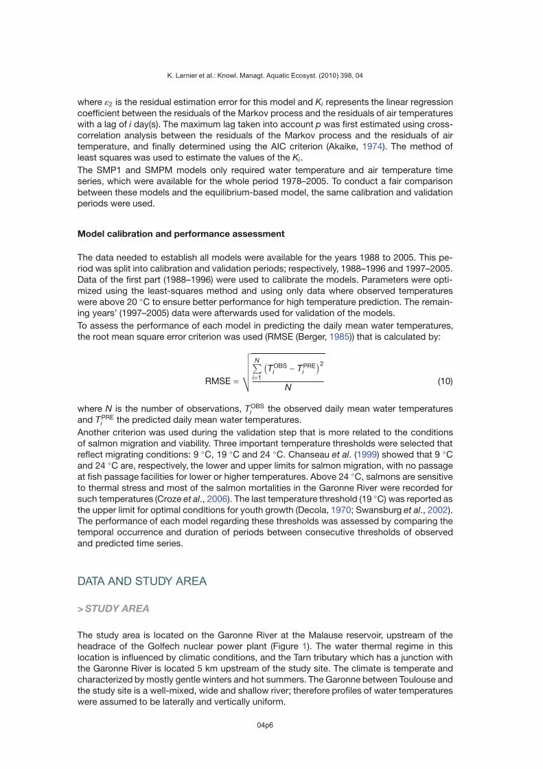
The study area is located on the Garonne River at the Malause reservoir, upstream of theheadrace of the Golfech nuclear power plant (Figure 1). The water thermal regime in thislocation is influenced by climatic conditions, and the Tarn tributary which has a junction withthe Garonne River is located 5 km upstream of the study site. The climate is temperate andcharacterized by mostly gentle winters and hot summers. The Garonne between Toulouse andthe study site is a well-mixed, wide and shallow river; therefore profiles of water temperatureswere assumed to be laterally and vertically uniform.

04p6


LamagistèreMalause

Study Site

Hydrological Station

Meteorological

Station LamagistèreMalause

Study Site

Hydrological Station

Meteorological

Station

Figure 1

Study site and locations of data stations. Adapted from EPTB Garonne website (http://www.

eptb-garonne.fr).

Figure 1Zone d’étude et localisation des stations de données – d’après une carte disponible sur le site de l’EPTBGaronne.

Data

Along our study reach a large amount of climatic and hydrologic data was gathered. Dailymean water temperature series in Malause were available from 1978 to 2005 from measure-ments in the headrace of the Golfech nuclear power plant performed by EDF1. Hydrologicaldata were available at the Lamagistère station of the Banque HYDRO2 that is 17 km down-stream of Malause. Mean daily discharges were available from 1967 with no uncertain ormissing data and mean daily water levels from 1988 with about 1% of uncertain data and lessthan 0.01% of missing data. Three-hourly meteorological data were gathered at the Agen andBlagnac weather stations of Météo-France3. Air temperatures were available at both stationsfor the years 1978 to 2005 with less than 0.01% of missing or uncertain data. Incident solarradiation (also referred to as insolation) data were only available at the Agen station, with fewmissing data (0.2%) from 1978 to 2005. Cloud cover and wind speed were only availableat the Blagnac station from 1992 but with numerous uncertain or missing data. Cloud coveruncertain data were about 8% (no missing data) and the wind speed time series presents

1 Électricité de France, http://www.edf.fr.2 Banque HYDRO, http://www.hydro.eaufrance.fr.3 Météo-France, http://www.meteofrance.com.

04p7


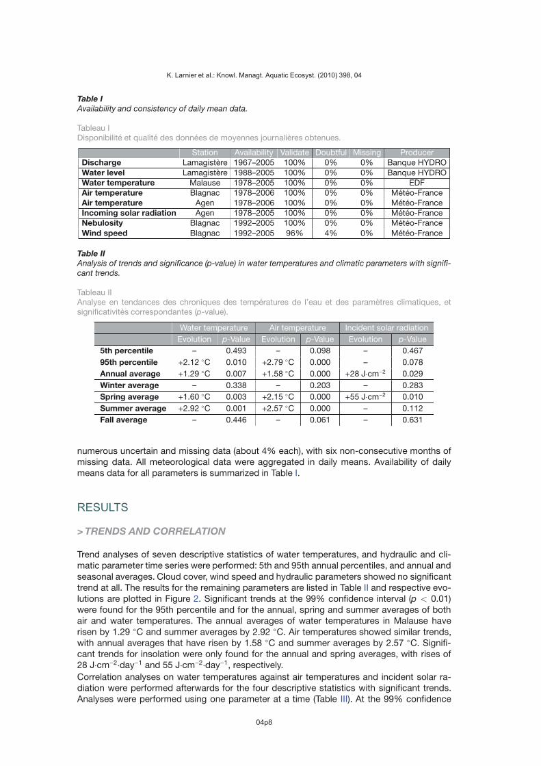
Table I

Availability and consistency of daily mean data.

Tableau IDisponibilité et qualité des données de moyennes journalières obtenues.

Station Availability Validate Doubtful Missing ProducerDischarge Lamagistère 1967–2005 100% 0% 0% Banque HYDROWater level Lamagistère 1988–2005 100% 0% 0% Banque HYDROWater temperature Malause 1978–2005 100% 0% 0% EDFAir temperature Blagnac 1978–2006 100% 0% 0% Météo-FranceAir temperature Agen 1978–2006 100% 0% 0% Météo-FranceIncoming solar radiation Agen 1978–2005 100% 0% 0% Météo-FranceNebulosity Blagnac 1992–2005 100% 0% 0% Météo-FranceWind speed Blagnac 1992–2005 96% 4% 0% Météo-France

Table II

Analysis of trends and significance (p-value) in water temperatures and climatic parameters with signifi-

cant trends.

Tableau IIAnalyse en tendances des chroniques des températures de l’eau et des paramètres climatiques, etsignificativités correspondantes (p-value).

Water temperature Air temperature Incident solar radiation

Evolution p-Value Evolution p-Value Evolution p-Value

5th percentile – 0.493 – 0.098 – 0.467

95th percentile +2.12 ◦C 0.010 +2.79 ◦C 0.000 – 0.078

Annual average +1.29 ◦C 0.007 +1.58 ◦C 0.000 +28 J·cm−2 0.029

Winter average – 0.338 – 0.203 – 0.283

Spring average +1.60 ◦C 0.003 +2.15 ◦C 0.000 +55 J·cm−2 0.010

Summer average +2.92 ◦C 0.001 +2.57 ◦C 0.000 – 0.112

Fall average – 0.446 – 0.061 – 0.631

numerous uncertain and missing data (about 4% each), with six non-consecutive months ofmissing data. All meteorological data were aggregated in daily means. Availability of dailymeans data for all parameters is summarized in Table I.

RESULTS

> TRENDS AND CORRELATION

Trend analyses of seven descriptive statistics of water temperatures, and hydraulic and cli-matic parameter time series were performed: 5th and 95th annual percentiles, and annual andseasonal averages. Cloud cover, wind speed and hydraulic parameters showed no significanttrend at all. The results for the remaining parameters are listed in Table II and respective evo-lutions are plotted in Figure 2. Significant trends at the 99% confidence interval (p < 0.01)were found for the 95th percentile and for the annual, spring and summer averages of bothair and water temperatures. The annual averages of water temperatures in Malause haverisen by 1.29 ◦C and summer averages by 2.92 ◦C. Air temperatures showed similar trends,with annual averages that have risen by 1.58 ◦C and summer averages by 2.57 ◦C. Signifi-cant trends for insolation were only found for the annual and spring averages, with rises of28 J·cm−2

·day−1 and 55 J·cm−2·day−1, respectively.

Correlation analyses on water temperatures against air temperatures and incident solar ra-diation were performed afterwards for the four descriptive statistics with significant trends.Analyses were performed using one parameter at a time (Table III). At the 99% confidence

04p8


0

10

20

30

1978 1983 1988 1993 1998 2003

Wate

r te

mp

era

ture

s (

°C)

95th percentileAnnual averagesSpring averagesSummer averages

0

10

20

30

1978 1983 1988 1993 1998 2003

Air

tem

pe

ratu

res (

°C)

0

400

800

1200

1978 1983 1988 1993 1998 2003

Incid

en

t so

lar

flu

x (

J·c

m2)

Figure 2.a Figure 2.b

Figure 2.c

Figure 2

Trends in water temperatures in Malause (Figure 2.a), air temperatures (Figure 2.b) and incident solar

radiation (Figure 2.c) at the Agen station.

Figure 2Tendance d’évolution des températures de l’eau à Malause (Figure 2.a), des températures de l’air(Figure 2.b) et de la radiation solaire à Agen (Figure 2.c).

Table III

Analysis of correlations and significance of water temperatures against air temperatures and incident

solar radiation.

Tableau IIIAnalyse des corrélations des températures de l’air et de la radiation solaire incidente avec les tempéra-tures de l’eau, et significativités correspondantes.

Air temperature Incident solar radiationCorrelation p-Value Correlation p-Value

95th percentile 0.85 0.000 – 0.344Annual average 0.83 0.000 – 0.507Spring average 0.78 0.000 0.58 0.001Summer average 0.87 0.000 0.48 0.010

interval, air temperature was the most significant predictor, that explained more than 75%of the variance of the water temperature descriptive statistics. Regarding high water tem-peratures (summer averages or the 95th percentile), air temperatures explained more than85% of the variance. The lowest calculated correlation coefficient was for spring averages(R2= 0.78). Insolation was significantly correlated with water temperatures only for spring

averages and summer averages (at the 99% confidence interval) but with correlation coef-ficients of less than 0.60. The best correlation coefficient was obtained for spring averages(R2= 0.58, p = 0.001).

04p9


Table IV

RMSE (◦C) calculated from observed and predicted daily mean water temperatures using the EQB model

for the years 1988–2005 in Malause.

Tableau IVErreurs-types (◦C) calculées entre les observations des températures moyennes journalières de l’eau etles estimations fournies par le modèle EQB sur la période 1988–2005.

Whole year TOBSw > 20 ◦C Whole year TOBS

w > 20 ◦C

1988 1.43 0.68 1997 1.23 1.06

1989 1.17 0.71 1998 1.07 0.76

1990 0.89 0.78 1999 1.11 0.61

1991 1.19 0.81 2000 1.25 1.07

1992 1.54 0.71 2001 1.05 0.84

1993 1.35 1.15 2002 1.40 1.21

1994 1.10 0.65 2003 1.56 1.74

1995 0.89 0.53 2004 1.41 1.41

1996 1.26 1.03 2005 1.61 1.72

1988–1996 1.22 0.81 1997–2005 1.31 1.22

Calibration period Validation period

> EQUILIBRIUM TEMPERATURE-BASED MODEL

Mean daily equilibrium temperatures showed a strong linear relation with daily mean air tem-peratures in Malause, with a calculated value of R2

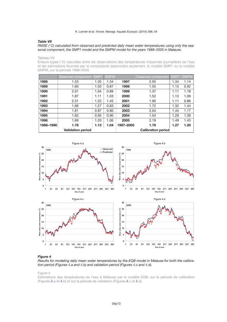
= 0.99. The EQB model was thereforecalibrated using data from the calibration period (1988–1996). The coefficients of the linearregression between estimated daily mean equilibrium temperatures and daily mean air tem-peratures were estimated as a1 = 1.12 and a2 = 0.44 ◦C. Using these values, the modifiedthermal coefficient was calculated at K′ = 0.56 s−1.On both the calibration period and validation period, RMSE were calculated for the overallperiod and for each year, both using all data and data with high observed daily mean watertemperatures (above 20 ◦C) only (Table IV). On the calibration period, the overall RMSE wascalculated at 1.22 ◦C and 0.81 ◦C for temperatures above 20 ◦C. Inter-annual comparisonshowed that the RMSE ranged from 0.89 ◦C (1990, 1995) to 1.54 ◦C (1992) using all data and0.53 ◦C (1995) to 1.15 ◦C (1993) for temperatures above 20 ◦C. On the validation period, theRMSE was calculated at 1.31 ◦C. Values calculated for each year ranged from 1.05 ◦C (2001)to 1.61 ◦C (2005). Regarding temperatures above 20 ◦C only, the RMSE ranged from 0.61 ◦C(1999) to 1.72 ◦C (2005) with an overall value calculated at 1.22 ◦C. The fitness of the resultscan also be assessed in Figure 4. The model showed good agreement on temperatures above20 ◦C, except for the year 2005 where temperatures around day 180 were overpredicted.Overpredictions were also noted for temperatures just below 20 ◦C, as for spring of the year1998.

> STOCHASTIC MODELS

The values calculated for χk and φk for the first two harmonics of equation (7) are listed in Ta-ble V. Comparison of the seasonal components of water and air temperatures indicated thatwater temperatures – apart from short-term variations – are always higher than air tempera-tures (see Figure 3). Moreover, the relation between interannual means was Tw = 1.12Ta+0.37.The seasonal component of water temperatures explained 92% of the deviance in the period1988–1996 and 84% in the period 1997–2005. Regarding air temperatures, the proportion ofdeviance explained by the seasonal components was 76% in the period 1988–1996 and 70%in the period 1997–2005. These values agree with those reported by Kothandaraman (1971).The maximum temperature for the long-term component of the stream water temperaturewas reached on day 226 (August 14) at a value of 23.8 ◦C.

04p10


0

5

10

15

20

25

30

0 50 100 150 200 250 300 350

Day of year

Te

mp

era

ture

(°C

)

Air temperature - 1st harmonic Air temperature - seasonal

Water temperature - 1st harmonic Water temperature - seasonal

Figure 3

First harmonics and complete seasonal components in air and water temperatures.

Figure 3Composantes saisonnières des chroniques de températures de l’air et de l’eau (complètes et premièresharmoniques seules).

Once the long-term variations were removed from the water temperature time series, theSMP1 and SMPM models were fitted on the residuals. The autocorrelation coefficients forthe water temperature residuals were calculated at R1 = 0.97 and R2 = 0.91. The Markovcoefficients were therefore calculated at A1 = 1.54 and A2 = −0.58.The thermal exchange coefficient of the SMP1 model was then calculated as 0.049 using datafor the validation period (1988–1996). The SMP1 model is therefore expressed as follows:

Rw(t) = 1.54Rw(t − 1) − 0.58Rw(t − 2) + 0.049Ra(t) + ε1(t). (11)

Root mean square errors between predicted and observed values were calculated on thecalibration period as well as for each year and for high observed water temperatures (Tables VIand VII). The RMSE was calculated as 1.13 ◦C when using all data and 0.95 ◦C for hightemperatures. Overall results were better than those obtained with the EQB model but RMSEcalculated for high temperatures were a little bit higher. Results also varied from year to year,with the RMSE ranging from 0.87 ◦C (1994) to 1.35 ◦C (1988) for overall data and from 0.49 ◦C(1995) to 1.32 ◦C (1993) for high temperatures. On the validation period, the RMSE rangedfrom 1.11 ◦C (1999, 2001) to 1.49 ◦C (2005) using all data and from 0.72 ◦C (1999) to 1.72 ◦C(2003) for temperatures above 20 ◦C, with values of 1.27 ◦C calculated on the whole validationperiod using both all data and temperatures above 20 ◦C.To establish the SMPM model, cross-correlation analysis between the residuals of the Markovprocess and the residuals of air temperatures revealed an exponential decrease in the cross-correlation coefficient when increasing the lag. The cross-correlation coefficients calculatedfor lags of 0 to 3 days were, respectively, 0.53, 0.41, 0.32 and 0.25. The analyses of the AICcriterion and significance of the regression coefficients showed that lags higher than 3 dayswere insignificant. Finally, the SMPM model is expressed as follows:

Rw(t) = 1.54Rw(t − 1) − 0.58Rw(t − 2) + 0.045Ra(t)+0.035Ra(t − 1) − 0.032Ra(t − 2) − 0.014Ra(t − 3) + ε2(t). (12)

This model clearly provided better results than the SMP1 model (Table VII). Moreover, it fittedbetter than the EQB model on the whole time series with the RMSE calculated at 1.04 ◦C

04p11


Table V

Coefficient values of seasonal (Eq. (10)) components for air and water temperatures.

Tableau VCoefficients des composantes saisonnières (Éq. (7)) des chroniques de températures de l’air et de l’eau.

Water temperature Air temperatureχ1 8.43 7.93φ1 2.67 2.79χ2 1.48 0.84φ2 –1.73 –1.50

Table VI

RMSE (◦C) calculated from observed and predicted daily mean water temperatures using the SMP1

model and the SMPM model for the years 1988–2005 in Malause.

Tableau VIErreurs-types (◦C) calculées entre les observations des températures moyennes journalières de l’eau etles estimations fournies par les modèle SMP1 et SMPM sur la période 1988–2005.

SMP1 SMPM

All data TOBSw > 20 ◦C All data TOBS

w > 20 ◦C

1988 1.35 0.94 1.34 0.90

Calibration period

1989 1.03 0.85 0.87 0.751990 1.04 0.83 0.89 0.721991 1.11 0.89 1.03 0.901992 1.22 0.89 1.45 1.021993 1.27 1.32 0.83 0.751994 0.87 0.79 0.80 0.681995 0.95 0.49 0.90 0.551996 1.20 1.25 1.06 0.821988–1996 1.13 0.95 1.04 0.79

1997 1.34 1.17 1.14 0.90

Validation period

1998 1.15 1.04 0.92 0.651999 1.11 0.72 1.18 0.562000 1.13 1.13 1.09 1.042001 1.11 0.94 0.86 0.852002 1.32 1.42 1.44 1.402003 1.44 1.72 1.17 0.962004 1.29 1.36 1.39 1.232005 1.49 1.64 1.43 1.291997–2005 1.27 1.27 1.20 1.01

on the calibration period (versus 1.20 ◦C for the EQB model and 1.13 ◦C for the SMP1 model)and 1.20 ◦C on the validation period (versus 1.31 ◦C for the EQB model and 1.27 ◦C for theSMP1 model). Results for temperatures above 20 ◦C were about the same as those obtainedwith the EQB model on the calibration period (0.79 ◦C versus 0.81 ◦C for the EQB model) andwere better than with the SMP1 model (0.95 ◦C). The RMSE ranged for this period between0.80 ◦C (1994) and 1.45 ◦C (1992) using all data and from 0.55 ◦C (1995) to 1.02 ◦C (1992)using temperatures above 20 ◦C only. For the validation period the SMPM model clearlyprovided better results for temperatures above 20 ◦C, with the RMSE calculated at 1.01 ◦C(versus 1.22 ◦C for the EQB model and 1.27 ◦C for the SMP1 model) and ranging from 0.56 ◦C(1999) to 1.40 ◦C (2002). Comparison between the EQB model and SMPM model predictionsfor the years 1992 and 2005 (Figures 4 and 5) clearly showed the better accuracy of theSMPM model at low temperatures. The end of the 2005 time series was particularly betterpredicted by the SMPM model than by the EQB model.

04p12


Table VII

RMSE (◦C) calculated from observed and predicted daily mean water temperatures using only the sea-

sonal component, the SMP1 model and the SMPM model for the years 1988–2005 in Malause.

Tableau VIIErreurs-types (◦C) calculées entre les observations des températures moyennes journalières de l’eauet les estimations fournies par la composante saisonnière seulement, le modèle SMP1 ou le modèleSMPM, sur la période 1988–2005.

Seasonal component SMP1 SMPM Seasonal component SMP1 SMPM

1988 1.53 1.35 1.34 1997 2.05 1.34 1.14

1989 1.60 1.03 0.87 1998 1.55 1.15 0.92

1990 2.01 1.04 0.89 1999 1.37 1.11 1.18

1991 1.87 1.11 1.03 2000 1.52 1.13 1.09

1992 2.31 1.22 1.45 2001 1.90 1.11 0.86

1993 1.66 1.27 0.83 2002 1.72 1.32 1.44

1994 1.61 0.87 0.80 2003 2.04 1.44 1.17

1995 1.62 0.95 0.90 2004 1.54 1.29 1.39

1996 1.69 1.20 1.06 2005 2.19 1.49 1.43

1988–1996 1.78 1.13 1.04 1997–2005 1.78 1.27 1.20

Validation period Calibration period

1990

0

5

10

15

20

25

30

1 31 61 91 121 151 181 211 241 271 301 331 361

Day of year

Me

an

daily

wa

ter

tem

pera

ture

(°C

)

Observed

Predicted1992

0

5

10

15

20

25

30

1 31 61 91 121 151 181 211 241 271 301 331 361

Day of year

Me

an

daily

wa

ter

tem

pera

ture

(°C

)

1999

0

5

10

15

20

25

30

1 31 61 91 121 151 181 211 241 271 301 331 361

Day of year

Me

an

daily

wa

ter

tem

pera

ture

(°C

)

2005

0

5

10

15

20

25

30

1 31 61 91 121 151 181 211 241 271 301 331 361

Day of year

Me

an

daily

wa

ter

tem

pera

ture

(°C

)


Figure 4.c Figure 4.d

Figure 4

Results for modeling daily mean water temperatures by the EQB model in Malause for both the calibra-

tion period (Figures 4.a and 4.b) and validation period (Figures 4.c and 4.d).

Figure 4Estimations des températures de l’eau à Malause par le modèle EQB, sur la période de calibration(Figures 4.a et 4.b) et sur la période de validation (Figures 4.c et 4.d).

04p13


1992

0

5

10

15

20

25

30

1 31 61 91 121 151 181 211 241 271 301 331 361

Day of year

Me

an

dail

y w

ate

r te

mp

era

ture

(°C

)

Observed

Predicted1995

0

5

10

15

20

25

30

1 31 61 91 121 151 181 211 241 271 301 331 361

Day of year

Me

an

daily

wa

ter

tem

pera

ture

(°C

)

1999

0

5

10

15

20

25

30

1 31 61 91 121 151 181 211 241 271 301 331 361

Day of year

Me

an

dail

y w

ate

r te

mp

era

ture

(°C

)

Observed

Predicted

2005

0

5

10

15

20

25

30

1 31 61 91 121 151 181 211 241 271 301 331 361

Day of year

Me

an

daily

wa

ter

tem

pera

ture

(°C

)





Figure 5

Results for modeling daily mean water temperatures by the stochastic SMPM model in Malause for both

the calibration period (Figures 5.a and 5.b) and validation period (Figures 5.c and 5.d).

Figure 5Estimations des températures de l’eau à Malause par le modèle stochastique SMPM, sur la période decalibration (Figures 5.a et 5.b) et sur la période de validation (Figures 5.c et 5.d).

> TEMPERATURE CONDITIONS FOR MIGRATION

The last evaluation of those models consisted of evaluating their propensity to predict thecrossing of the three thresholds of water temperature related to salmon conditions for migra-tion and viability. The time locations of the corresponding periods are plotted in Figure 6. Inthis figure, short-lasting threshold crossings (less than 7 days) were erased to improve clarity.Both models showed good accuracy, particularly in predicting the 24 ◦C threshold crossings.Some large differences were, however, noted, as for the first crossing of the 19 ◦C thresholdin the year 1999. Distribution of errors between predicted and observed temperature werecalculated for each threshold and for days where crossings were not well predicted (Figure 7).Except for the 19 ◦C threshold, about 80% of errors were in the range [–2 ◦C; 2 ◦C]. For the9 ◦C and 24 ◦C thresholds, SMPM performed slightly better with, respectively, 87% and 84%of absolute errors less than 2 ◦C (versus 82% and 77% for the EQB model). On the contrary,the 9 ◦C threshold crossing was better predicted by the EQB with 57% of absolute errors lessthan 2 ◦C (versus 52% for the SMPM model).

DISCUSSION

Water temperatures in streams can be related to numerous factors such as climate, hydraulicregimes, bed topography, and others (Caissie, 2006; Webb et al., 2008). Deterministic modelsusing many factors have been used in the literature and proved to efficiently predict watertemperatures (Sinokrot and Stefan, 1984; Kim and Chapra, 1997; Webb and Zhang, 1999;

04p14


Figure 6

Comparison between observed and predicted time location of temperature conditions for spawning.

Favorable conditions are represented in green.

Figure 6Comparaison entre les observations et les estimations des occurrences temporelles liées aux conditionsde migration. Les périodes favorables sont représentées en vert.

Marcé and Armengol, 2008). Using those models, however, requires lots of data and com-putational resources. Such models are consequently not easy to use for practitioners. Thisstudy was therefore conducted on the Garonne River to assess the performance of statisti-cal models to predict daily mean water temperatures and particularly high temperatures thatimpact on aquatic ecosystems.

Trend analyses revealed that water temperature evolution was closely similar to that of airtemperatures. Similar results were reported for two large rivers in France, the Loire River(Moatar and Gailhard, 2006) and the Rhône River (Poirel et al., 2008). Such similarities tendto indicate that water temperature in large rivers in France is mainly influenced by climaticconditions and particularly air temperatures. Solar radiation was also noted to be correlatedwith the water temperature but using this factor as a predictor would potentially have resultedin statistical inadequacies associated with multicollinearity. Therefore, using models relyingon the relation between air and water temperatures seemed to be accurate for the GaronneRiver case.

The first model used in this study was based on the equilibrium temperature concept. Theequilibrium temperature reflects the energy budget of the stream and therefore is a functionof many meteorological factors. It has been shown that the equilibrium temperature could beexpressed as a simple linear function of air temperatures for temperate regions (Caissie et al.,2005). This assumption was verified for the Garonne River, with good agreement between airtemperatures and the equilibrium temperature (R2

= 0.99). The a1 coefficient was optimizedat a value of 1.12. This value was similar to that reported by Caissie et al. (2005) for the Little

04p15


0%

25%

50%

75%

]- ;-4]

]-4;-3

]

]-3;-2

]

]-2; 1

]

]-1; 0

]

] 0; 1

]

] 1; 2

]

] 2; 3

]

] 3; 4

]

] 4; +

[

EQB SMPM

0%

10%

20%

30%

40%

]- ;-4]

]-4;-3

]

]-3;-2

]

]-2; 1

]

]-1; 0

]

] 0; 1

]

] 1; 2

]

] 2; 3

]

] 3; 4

]

] 4; +

[

EQB SMPM

0%

10%

20%

30%

40%

50%

]- ;-4]

]-4;-3

]

]-3;-2

]

]-2; 1

]

]-1; 0

]

] 0; 1

]

] 1; 2

]

] 2; 3

]

] 3; 4

]

] 4; +

[

EQB SMPM


Figure 7.c

Figure 7

Distribution of discrepancies between predictions and observations for days where crossings of thresh-

olds were not accurately predicted.

Figure 7Répartition des erreurs entre estimations et observations pour les jours où les franchissements de seuilne sont pas correctement reproduits par les modèles.

Southwest Miramichi River (New Brunswick, Canada). Values of this coefficient higher than 1reflect that the river is well exposed to other meteorological factors than air temperatures (i.e.

solar radiation, etc.) which was the case of the Garonne river due to its wideness. The a2

coefficient, however, was not zero, which differs from the results reported by Caissie et al.The thermal coefficient K′ was calculated at 0.71 and agreed with that of the Little SouthwestMiramichi River.

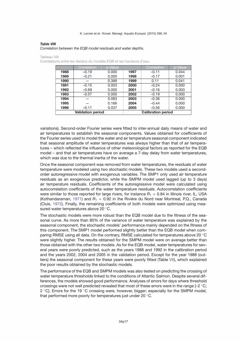
The results obtained with the equilibrium-based model were similar to those reported in otherstudies, with values of RMSE calculated at 1.22 ◦C on the calibration period and 1.31 ◦Con the validation period. Regarding temperatures above 20 ◦C only, slightly better valuesof 0.81 ◦C on the calibration period and 1.22 ◦C on the validation period were obtained.This model was therefore sensitive to the data used for calibration. Inter-annual comparisonalso indicated that estimations for several years were poorly estimated. Except for the year1988, whose measured water temperature time series contained outliers (caused by mea-surement failures), correlations between the model residuals and water depths were foundto be strong for those years, whereas poor correlations were calculated for years with goodresults (Table VIII). The EQB model was therefore sensitive to water depths and approximat-ing B/A with 1/h could be debated. Another simplification – neglecting diffusive and con-vective terms – could also be too restrictive. Significant floods with discharge of more than5000 m3

·s−1 happen in this river. During such floods, the importance of convective terms mustnot be negligible.

Stochastic modeling consisted of separating water temperatures and air temperatures intotwo components: a seasonal component (long-term variations) and residuals (short-term

04p16


Table VIII

Correlation between the EQB model residuals and water depths.

Tableau VIIICorrélations entre les résidus du modèle EQB et les hauteurs d’eau.

Correlation p-Value Correlation p-Value1988 –0.19 0.000 1997 –0.11 0.0441989 –0.21 0.000 1998 –0.17 0.0011990 — 0.389 1999 0.11 0.0411991 –0.15 0.003 2000 –0.24 0.0001992 –0.69 0.000 2001 –0.16 0.0031993 –0.57 0.000 2002 –0.19 0.0001994 — 0.083 2003 –0.36 0.0001995 — 0.166 2004 –0.44 0.0001996 –0.11 0.037 2005 –0.56 0.000

Validation period Calibration period

variations). Second-order Fourier series were fitted to inter-annual daily means of water andair temperatures to establish the seasonal components. Values obtained for coefficients ofthe Fourier series used to model the water and air temperature seasonal component indicatedthat seasonal amplitude of water temperatures was always higher than that of air tempera-tures – which reflected the influence of other meteorological factors as reported for the EQBmodel – and that air temperatures have on average a 7-day delay from water temperatures,which was due to the thermal inertia of the water.

Once the seasonal component was removed from water temperatures, the residuals of watertemperature were modeled using two stochastic models. These two models used a second-order autoregressive model with exogenous variables. The SMP1 only used air temperatureresiduals as an exogenous predictor, while the SMPM model used lagged (up to 3 days)air temperature residuals. Coefficients of the autoregressive model were calculated usingautocorrelation coefficients of the water temperature residuals. Autocorrelation coefficientswere similar to those reported for large rivers, for instance R1 = 0.84 in Illinois river, IL, USA(Kothandaraman, 1971) and R1 = 0.92 in the Rivière du Nord near Montreal, P.Q., Canada(Cluis, 1972). Finally, the remaining coefficients of both models were optimized using mea-sured water temperatures above 20 ◦C.

The stochastic models were more robust than the EQB model due to the fitness of the sea-sonal curve. As more than 80% of the variance of water temperature was explained by theseasonal component, the stochastic models’ performance mainly depended on the fitness ofthis component. The SMP1 model performed slightly better than the EQB model when com-paring RMSE using all data. On the contrary, RMSE calculated for temperatures above 20 ◦Cwere slightly higher. The results obtained for the SMPM model were on average better thanthose obtained with the other two models. As for the EQB model, water temperatures for sev-eral years were poorly predicted, such as the years 1988 and 1992 in the calibration periodand the years 2002, 2004 and 2005 in the validation period. Except for the year 1988 (out-liers) the seasonal component for these years were poorly fitted (Table VII), which explainedthe poor results obtained by the stochastic models.

The performance of the EQB and SMPM models was also tested on predicting the crossing ofwater temperature thresholds linked to the conditions of Atlantic Salmon. Despite several dif-ferences, the models showed good performance. Analyses of errors for days where thresholdcrossings were not well predicted revealed that most of these errors were in the range [–2 ◦C;2 ◦C]. Errors for the 19 ◦C crossing were, however, bigger; especially for the SMPM model,that performed more poorly for temperatures just under 20 ◦C.

04p17


CONCLUSION

Both approaches used in this study could be useful for practitioners. Despite being appliedto a complex study area (reservoir and influence of tributary), these simplified models showedgood accuracy in predicting high water temperatures of the Garonne River in Malause. Aswater and air temperatures are relatively inexpensive to measure, statistical models are goodalternatives to deterministic models that require much more data. In our study, equilibriumtemperatures were established from meteorological parameters, and values of the linear re-gression between equilibrium temperatures and air temperatures were calculated afterwards.However, it should be possible to establish the model directly using only air and water temper-atures and an optimization method in order to use only air temperatures, water temperaturesand water depths. Furthermore, using real values of top width and wetted area or non-linearregression would probably result in better prediction, as well as multiplying each thermalflux by a calibration factor (Caissie et al., 2007) to slightly modify their respective influences.Regarding the stochastic models, performance was mainly dependent on the fitness of theseasonal component. Therefore, further research is needed to explore the advantages of us-ing variable coefficients for this component. Finally, as the meteorological station was located17 km downstream of the study site, potential improvements could also be made by alter-natively using microclimate data (Benyahya et al., 2010), particularly in determination of heatfluxes for the EQB model.Each model could have different usage for practitioners. As the EQB predicts water tem-peratures from climatic conditions, this model could be useful to assess the evolution ofthe thermal regime of the Garonne River under climate change. Using regional data derivedfrom Global Circulation Model (GCM) outputs, water temperatures could be calculated forfuture years. On the contrary, the stochastic models used in this study require knowledgeof past water temperature values. These models are therefore more suitable for short-termpredictions.

REFERENCES

Ahmadi-Nedushan B., St-Hilaire A., Ouarda T.B.M.J., Bilodeau L., Robichaud E., Thiemonge N. andBobee B., 2007. Predicting river water temperatures using stochastic models: case study of theMoisie River (Quebec, Canada). Hydrol. Process., 21, 21–34.

Akaike H., 1974. A new look at the statistical model identification. IEEE Trans. Automat. Contr., 19,716–723.

Alabaster J.S., 1967. The survival of salmon (Salmo salar L.) ans sea trout (S. trutta L.) in fresh and salinewater at high temperatures. Water Res., 1, 717–730.

Benyahya L., Caissie D., St-Hilaire A., Ouarda T.B.M.J. and Bobee B., 2007a. A review of statisticalwater temperature models. Can. Water Resources J., 32, 179–192.

Benyahya L., St-Hilaire A., Ouarda T.B.M.J., Bobee B. and Ahmadi-Nedushan B., 2007b. Modelingof water temperatures based on stochastic approaches: case study of the Deschutes River.J. Environ. Eng. Sci., 6, 437–448.

Benyahya L., Caissie D., El-Jabi N. and Satish M.G., 2010. Comparison of microclimate vs. remotemeteorological data and results applied to a water temperature model (Miramichi River, Canada).J. Hydrol., 380, 247–259.

Berger J.O., 1985. Certain Standard Loss Functions. In: Statistical decision theory and BayesianAnalysis, 2nd edn., Springer-Verlag, New York, 60–64.

Caissie D., 2006. The thermal regime of rivers: a review. Freshw. Biol., 51, 1389–1406.

Caissie D., El-Jabi N. and St-Hilaire A., 1998. Stochastic modelling of water temperatures in a smallstream using air to water relations. Can. J. Civ. Eng., 25, 250–260.

Caissie D., Satish M.G. and El-Jabi N., 2005. Predicting river water temperatures using the equilibriumtemperature concept with application on Miramichi River catchments (New Brunswick, Canada).Hydrol. Process., 19, 2137–2159.

04p18


Caissie D., Satish M.G. and El-Jabi N., 2007. Predicting water temperatures using a deterministic model:Application on Miramichi River catchments (New Brunswick, Canada). J. Hydrol., 336, 303–315.

Chanseau M., Croze O. and Larinier M., 1999. Impact des aménagements sur la migration anadrome dusaumon atlantique (Salmo salar L.) sur le gave de Pau (France). Bull. Fr. Pêche Piscic., 353-354,211–237.

Chenard J.F. and Caissie D., 2008. Stream temperature modelling using artificial neural networks: appli-cation on Catamaran Brook, New Brunswick, Canada. Hydrol. Process., 22, 3361–3372.

Cluis D.A., 1972. Relationship between stream water temperature and ambient temperature – a simpleautoregressive model for mean daily stream water temperature fluctuations. Nordic Hydrology, 3,65–71.

Croze O., Blot E., Delmas F., Alesina R., Jourdan H., Bau F. and Breinig T., 2006. Suivi de la qualité del’eau de la Garonne lors de la migration anadrome du saumon en amont de Golfech. RA06.04,GHAAPE, Toulouse.

Decola J.N., 1970. Water quality requirements for Atlantic salmon. CWT–10-16; PB–230733, FederalWater Quality Administration, Needham Heights, New England Basins Office.

Edinger J.E., Duttweiler D.W. and Geyer J.C., 1968. The response of water temperatures to meteorolog-ical conditions. Water Resour. Res., 4, 1137–1143.

El-Jabi N., El-Kourdahi G. and Caissie D., 1995. Modélisation stochastique de la température de l’eauen rivière. Revue des Sciences de l’Eau, 8, 77–95.

Elliott J.M., 1991. Tolerance and resistance to thermal stress in juvenile Atlantic salmon, Salmo salar.Freshw. Biol., 25, 61–70.

Erickson T.R. and Stefan H.G., 2000. Linear air/water temperature correlations for streams during openwater periods. J. Hydrol. Eng., 5, 317–321.

Fairchild W.L., Swansburg E.O., Arsenault J.T. and Brown S.B., 1999. Does an association betweenpesticide use and subsequent declines in catch of Atlantic salmon (Salmo salar) represent a caseof endocrine disruption? Environ. Health Perspect., 107, 349–357.

Kim K.S. and Chapra S.C., 1997. Temperature model for highly transient shallow streams. J. Hydraul.

Eng., 123, 30–40.

Kothandaraman V., 1971. Analysis of water temperature variations in large river. Journal of the Sanitary

Engineering Division-ASCE, 97, 19–31.

Leopold L.B., Wolman M.G. and Miller J.P., 1964. Fluvial process in Geomorphology, W.H. Freeman andCo., San Francisco.

Marcé R. and Armengol J., 2008. Modelling river water temperature using deterministic, empirical, andhybrid formulations in a Mediterranean stream. Hydrol. Process., 22, 3418–3430.

Marcotte N. and Duong V.-L., 1973. Le calcul de la température de l’eau des rivières. J. Hydrol., 18,273–287.

Moatar F. and Gailhard J., 2006. Water temperature behaviour in the River Loire since 1976 and 1881.C. R. Geosci., 338, 319–328.

Mohseni O. and Stefan H.G., 1999. Stream temperature air temperature relationship: a physical inter-pretation. J. Hydrol., 218, 128–141.

Mohseni O., Stefan H.G. and Erickson T.R., 1998. A nonlinear regression model for weekly stream tem-peratures. Water Resour. Res., 34, 2685–2692.

Morin G. and Couillard D., 1990. Predicting river temperatures with a hydrological model. In:Encyclopedia of Fluid Mechanic, Surface and Groundwater Flow Phenomena, Golf PublishingCompany, Houston, 171–209.

Pilgrim J.M., Fang X. and Stefan H.G., 1998. Stream temperature correlations with air temperatures inMinnesota: implications for climate warning. J. Am. Water Resour. Assoc., 34, 1109–1121.

Poirel A., Lauters F. and Desaint B., 2008. 1977–2006 : Trente années de mesures des températures del’eau dans le Bassin du Rhône. Hydroécol. Appl., 16, 191–213.

Raphael J.M., 1962. Prediction of temperature in rivers and reservoirs. Journal of the Power Division,88, 157–181.

Sinokrot B.A. and Stefan H.G., 1984. Stream water-temperature sensitivity to weather and bed param-eters. J. Hydraul. Eng., 120, 722–736.

04p19


Sinokrot B.A. and Stefan H.G., 1993. Stream Temperature Dynamics – Measurements and Modeling.Water Resour. Res., 29, 2299–2312.

Sinokrot B.A. and Stefan H.G., 1994. Stream water-temperature sensitivity to weather and bed param-eters. J. Hydraul. Eng., 120, 722–736.

Stefan H.G. and Preud’homme E.B., 1993. Stream temperature estimation from air temperature. J. Am.

Water Resour. Assoc., 29, 27–45.

Swansburg E., Chaput G., Moore D., Caissie D. and El-Jabi N., 2002. Size variability of juvenile Atlanticsalmon: links to environmental conditions. J. Fish Biol., 61, 661–683.

Torgersen C.E., Faux R.N., McIntosh B.A., Poage N.J. and Norton D.J., 2001. Airborne thermal remotesensing for water temperature assessment in rivers and streams. Remote Sens. Environ., 76, 386–398.

Webb B.W. and Zhang Y., 1999. Water temperatures and heat budgets in Dorset chalk water courses.Hydrol. Process., 13, 309–321.

Webb B.W., Hannah D.M., Moore R.D., Brown L.E. and Nobilis F., 2008. Recent advances in stream andriver temperature research. Hydrol. Process., 22, 902–918.

Wilkie M.P., Brobel M.A., Davidson K., Forsyth L. and Tufts B.L., 1997. Influences of temperature uponthe postexercise physiology of Atlantic salmon (Salmo salar). Can. J. Fish. Aquatic Sci., 54, 503–511.

04p20

Documents

Open Archive TOULOUSE Archive Ouverte (OATAO) · Ces modèles ont été calibrés sur la première moitié de la pé- riode 1988–2005en utilisant les données de température supérieures