OPEN ACCESS entropy

Entropy 2014, 16, 2869-2889; doi:10.3390/e16052869OPEN ACCESS

entropyISSN 1099-4300

www.mdpi.com/journal/entropy

Article

A Maximum Entropy Approach to Assess Debonding inHoneycomb Aluminum PlatesViviana Meruane *, Valentina del Fierro and Alejandro Ortiz-Bernardin

Department of Mechanical Engineering, Universidad de Chile, Beauchef 850, Santiago, Chile;E-Mails: [email protected] (V.F.); [email protected] (A.O.-B.)

* Author to whom correspondence should be addressed; Email: [email protected];Tel: +56-2-29784597.

Received: 22 March 2014; in revised form: 12 May 2014 / Accepted: 21 May 2014 /Published: 23 May 2014

Abstract: Honeycomb sandwich structures are used in a wide variety of applications.Nevertheless, due to manufacturing defects or impact loads, these structures can be subject toimperfect bonding or debonding between the skin and the honeycomb core. The presence ofdebonding reduces the bending stiffness of the composite panel, which causes detectablechanges in its vibration characteristics. This article presents a new supervised learningalgorithm to identify debonded regions in aluminum honeycomb panels. The algorithmuses a linear approximation method handled by a statistical inference model based on themaximum-entropy principle. The merits of this new approach are twofold: training isavoided and data is processed in a period of time that is comparable to the one of neuralnetworks. The honeycomb panels are modeled with finite elements using a simplifiedthree-layer shell model. The adhesive layer between the skin and core is modeled usinglinear springs, the rigidities of which are reduced in debonded sectors. The algorithmis validated using experimental data of an aluminum honeycomb panel under differentdamage scenarios.

Keywords: Sandwich structures; debonding; honeycomb; damage assessment;maximum-entropy principle; linear approximation

Entropy 2014, 16 2870

1. Introduction

The applications of sandwich structures continue to increase rapidly and range from satellites,spacecrafts, aircrafts, ships, automobiles, rail cars, wind energy systems to bridge construction, amongothers [1]. Sandwich panels typically consist of two thin face sheets or skins and a lightweightthicker core, which is sandwiched between two faces to obtain a structure of superior bending stiffness.Nevertheless, due to manufacturing defects or impact loads, these structures can experience imperfectbonding or debonding between the skin and the honeycomb core. Debonding in a sandwich structuremay severely degrade its mechanical properties, which can produce a catastrophic failure of the overallstructure. Therefore, it is important to detect the presence of debonding at an early stage.

A disadvantage of sandwich structures is that their structural failures, especially in the core, cannotalways be detected by traditional non-destructive detection methods. A global technique calledvibration-based damage detection has been rapidly expanding over the last few years [2]. The basicidea is that vibration characteristics (natural frequencies, mode shapes, damping, frequency responsefunction, etc.) are functions of the physical properties of the structure. Thus, changes to the materialand/or geometric properties due to damage will cause detectable changes in the vibrations characteristics.A debonded region in a sandwich structure is equivalent to a delamination in composite laminates.Many studies have demonstrated that vibration characteristics are sensitive to delamination even if thedelamination is located in hidden or internal areas [3,4]. Nevertheless, there have only been a few studiesrelated to the debonding of sandwich structures [5–10].

Vibration-based damage assessment methods are classified as model-based or non-model based.Non-model-based methods detect damage by comparing the measurements from the undamaged anddamaged structures, whereas model-based methods locate and quantify damage by correlating ananalytical model with test data from a damaged structure. Additionally, model-based methods areparticularly useful for predicting the system response to new loading conditions and/or new systemconfigurations (damage states), allowing damage prognosis [11]. Model-based damage assessmentrequires the solution of a nonlinear inverse problem, which can be accomplished using supervisedlearning algorithms as neural networks or by global optimisation algorithms. The most successfulapplications of vibration-based damage assessment are model updating methods based on globaloptimization algorithms [12–16]. Nevertheless, these algorithms are exceedingly slow and the damageassessment process is achieved via a costly and time-consuming inverse process, which presents anobstacle for real-time health monitoring applications.

Supervised learning algorithms are an alternative to model updating. The objective of supervisedlearning is to estimate the structure’s health based on current and past samples. Supervised learningcan be divided into two classes: parametric and non-parametric. Parametric approaches assumed astatistical model for the data samples. A popular parametric approach is to model each class density asGaussian [17]. Nonparametric algorithms do not assume a structure for the data. The most frequentlynonparametric algorithms used in damage assessment are artificial neural networks [18–24]. A trainedneural network can potentially detect, locate and quantify structural damage in a short period of time.Hence, it can be used for real-time damage assessment. Although once a neural network is already

Entropy 2014, 16 2871

trained it can process data very quickly, the slow learning speed and the large number of parameters thatneed to be tuned within the training stage have been a major bottleneck in their application [25].

A new nonparametric method for supervised learning was presented by Gupta et al. [26,27]. Thismethod generalized linear approximation by using the maximum-entropy (max-ent) principle [28] forstatistical inference. A similar approach was adopted by Erkan [29] for semi-supervised learningproblems, where a decision rule is to be learned from labelled and unlabeled data. By using max-entmethods, training is avoided and data is processed in a period of time that is comparable to the one ofneural networks. In addition, it only requires one parameter to be selected. Hence, max-ent methodsbecome very appealing for real-time health monitoring applications. Gupta [26] demonstrated theapplication of the max-ent approach to color management and gas pipeline integrity problems. In thepresent paper, we demonstrate the applicability of max-ent methods in structural damage assessment.

The primary contribution of this research is the development of a real-time damage assessmentalgorithm for honeycomb panels that uses a linear approximation method in conjunction with the modeshapes and natural frequencies of the structure. The linear approximation is handled by a statisticalinference model based on the maximum-entropy principle [28]. The honeycomb panels are modeledwith finite elements using a simplified three-layer shell model. The adhesive layer between the skinand core is modeled using linear springs, with reduced rigidities for the debonded sectors. Thealgorithm is validated using experimental data from an aluminum honeycomb panel containing differentdamage scenarios.

The remainder of this work is structured as follows: Section 2 introduces the proposed damageassessment algorithm and provides previous research on the max-ent linear approximation method.Section 3 describes the construction of the numerical model for the honeycomb sandwich panel.Section 4 presents the experimental structure and the correlation between the experimental and numericalmodes. Section 5 describes the setting up of the database. Section 6 presents the case studies and thedamage assessment results. Finally, conclusions and forthcoming work are presented in Section 7.

2. Damage Assessment Using Linear Approximation with Maximum Entropy

The main problem of vibration-based damage assessment is to ascertain the presence, location andseverity of structural damage given a structure’s dynamic characteristics. This principle is illustrated inFigure 1; the vibration characteristics of the structure, which in this case correspond to mode shapes andnatural frequencies, act as the input to the algorithm, and the outputs are the damage indices of eachelement in the structure.

Figure 1. Principle of a vibration-based damage assessment algorithm.

Experimental structure

Vibrationcharacteristics

Damageindices

DamageSensors Damage

assessmentalgorithm

X Ŷ

Entropy 2014, 16 2872

Let the observation vector Yi = {Y i1 , Y

i2 , . . . , Y

im} ∈ Rm represent the ith damage state of the

structure. Let the feature vector Xi = {X i1, X

i2, . . . , X

in} ∈ Rn represent a set of vibration characteristics

of the structure associated with the damage state Yi. The variables X and Y have joint distribution PX,Y .Let a set of k independent and identically distributed samples be drawn from PX,Y . These samplesrepresent the database (X1,Y1), (X2,Y2), ..., (Xk,Yk). The central problem in supervised learning isto form an estimate of PY |X , i.e. given a certain feature X, estimate the corresponding observation Y.Let Y denote the estimated value of Y.

Linear approximation takes the N nearest neighbors to a test point X and uses a linear combinationof them to represent X as

X =N∑i=1

wi(X)Xi(X),N∑i=1

wi(X) = 1, (1)

where w1, w2, . . . , wN are weighting functions, and X1(X),X2(X), . . . ,XN(X) are the N closestneighbors to a test point X out of the database set. The equations given in (1) can be expressed asthe following system of linear equations:

Aw = b, w ≥ 0, (2)

with A =

X1

1 X21 . . . XN

1

X12 X2

2 . . . XN2

...... . . . ...

X1n X2

n . . . XNn

1 1 . . . 1

(n+1)×N

, b =

X1

X2

...Xn

1

(n+1)×1

, w =

w1

w2

...wN

N×1

.

After w is obtained from Equation (2), Y is estimated as

Y =N∑i=1

wi(X)Yi(X), (3)

where Y1(X),Y2(X), . . . ,YN(X) are the corresponding observations to the N selected neighbors.Typically, the system of Equation (2) is undetermined, and its solution is tackled via a constrainedoptimization technique of the family of least-squares (nonnegative least-squares [30]). An alternativethat provides the least-biased solution is obtained via the maximum-entropy (max-ent) variationalprinciple [28]. Recently, max-ent methods have become quite popular in the computational mechanicscommunity as a powerful tool for numerical solution of PDEs [31–39], and their applications in thesolution of ill-posed inverse problems have also been explored [40,41].

The notion of entropy in information theory was introduced by Shannon as a measure ofuncertainty [42]. Later, on using the Shannon entropy, Jaynes [28] postulated the maximum-entropyprinciple as a rationale means for least-biased statistical inference when insufficient information isavailable. The maximum-entropy principle is suitable to find the least-biased probability distributionwhen there are fewer constraints than unknowns and is posed as follows:

Consider a set ofN discrete events {x1, . . . , xN}. The possibility of each event is pi = p(xi) ∈ [0, 1]

with uncertainty − ln pi. The Shannon entropy H(p) = −∑N

i=1 pi ln pi is the amount of uncertainty

Entropy 2014, 16 2873

represented by the distribution {p1, . . . , pN}. The least-biased probability distribution and the one thathas the most likelihood to occur is obtained via the solution of the following optimization problem(maximum-entropy principle):

maxp∈RN

+

[H(p) = −

N∑i=1

pi ln (pi)

], (4a)

subject to the constraints:

N∑i=1

pi = 1,N∑i=1

pigr(xi) =< gr(x) >, (4b)

where RN+ is the non-negative orthant and < gr(x) > is the known expected value of functions gr(x)

(r = 0, 1, . . . ,m), with g0(x) = 1 being the normalizing condition.The optimization problem (4) assigns probabilities to every xi in the set. Now, assume that the

probability pi has an initial guessmi known as a prior, which reduces its uncertainty to− ln pi+lnmi =

− ln(pi/mi). An alternative problem can be formulated by using this prior in (4) [43]:

maxp∈Rn

+

[H(p) = −

N∑i=1

pi ln

(pimi

)], (5a)


n∑i=1

pi = 1,n∑

i=1

pigr(xi) =< gr(x) > . (5b)

In (5), the variational principle associated with∑N

i=1 pi ln(

pimi

)is known as the principle of minimum

relative (cross) entropy [44,45]. Depending upon the prior employed, the optimization problem (5) willfavor some xi in the set by assigning more probability to them, and eventually, assigning non-zeroprobability (pi > 0) to a selected number of xi (i < N ) in the set. It can be easily seen that if the prioris constant, the Shannon-Jaynes entropy functional (4) is recovered as a particular case.

Because of its general character and flexibility, we adopt the relative entropy approach for ourproblem, where the probability pi is replaced with the weighting function wi of the linear approximationproblem posed in Equation (1). This reads:

maxw∈RN

+

[H(w) = −

N∑i=1

wi(X) ln

(wi(X)

mi(X)

)], (6a)


N∑i=1

wi(X)Xi = 0,N∑i=1

wi(X) = 1, (6b)

Entropy 2014, 16 2874

where Xi = Xi − X has been introduced as a shifted measure for stability purposes. A typical priordistribution is the smooth Gaussian [31]

mi(X) = exp(−βi‖Xi‖2), (7)

where βi = γ/h2i ; γ is a parameter that controls the radius of the Gaussian prior at Xi, and thereforeits associated weight function; and hi is a characteristic n−dimensional Euclidean distance betweenneighbors that can be distinct for each Xi. In view of the optimization problem posed in (6) forsupervised learning, maximizing the entropy chooses the weight solution that commits the least to anyone in the database samples [27].

The solution of the max-ent optimization problem is handled by using the procedure of Lagrangemultipliers, which yields [43]:

wi(X) =Zi(X;λ∗)

Z(X;λ∗), Zi(X;λ∗) = mi(X) exp(−λ∗ · Xi), (8)

where Z(X;λ∗) =∑

j Zj(X;λ∗), Xi = [X i1 . . . X

iN ]

T and λ∗ = [λ∗1 . . . λ∗N ]

T.In Equation (8), the Lagrange multiplier vector λ∗ is the minimizer of the dual optimization problem

posed in Equation (6) [43]:λ∗ = arg min

λ∈RNlnZ(X;λ), (9)

which gives rise to the following system of nonlinear equations:

f(λ) = ∇λ lnZ(λ) = −N∑i

wi(X)Xi = 0, (10)

where∇λ stands for the gradient with respect to λ. Once the converged λ∗ is found, the weight functionsare computed from Equation (8).

3. Numerical Model

Figure 2 shows a scheme for a honeycomb sandwich panel, consisting of two thin face sheets orskins and a honeycomb core, which are bonded together by an adhesive layer. The panel can bemodeled by a detailed 3D finite element model, but the computational effort increases very rapidlyas the number of cells increases. Therefore, it is more convenient to develop equivalent simplifiedmodels for the honeycomb core to reduce the required computational time. Burton and Noor [46]studied the performance of nine different modeling approaches based on two-dimensional shell theoriesto predict the static response of sandwich panels. The results were compared to those from a detailedthree-dimensional model. Their study showed that the global response can be accurately predictedby discrete three-layer models, predictor-corrector approaches and even first-order shear deformationtheory, provided that proper values for the shear correction factors are used. According to Birman andBert [47], a key factor in the practical application of the first-order shear deformation theory is thedetermination of the shear correction factor. The analysis presented by these researchers concludedthat the shear correction factor should be taken with a value equal to unity for sandwich structures,as a first approximation. The work presented by Burton and Noor [48] showed that continuum layer

Entropy 2014, 16 2875

models for the honeycomb core provide solutions that are close to those calculated by using detailedfinite element models. Tanimoto et al. [49] used beam elements to model the honeycomb core and theadhesive layer. The proposed model was validated by experimental vibration tests. Burlayenko andSadowski [50] performed an analysis of sandwich plates with hollow and foam-filled honeycomb coresusing a commercially available finite element code. The sandwich plates were modeled on the basis of asimplified three-layered continuum model using a mixed shell/solid approach.

Consequently, the prediction of the dynamic response of the honeycomb panels can be accomplishedby equivalent continuum models. In the present study, the honeycomb panels are modeled with finiteelements using a simplified three-layer shell model and the adhesive layer between the skin and core ismodeled using linear springs. Because the properties of the skin are known, the attention is focused onmodeling the effective properties of the adhesive layer and the core material.

Figure 2. Scheme of a honeycomb sandwich panel.

Adhesive layer

Skin

Honeycomb core

A debonded region between the skin and core of a honeycomb panel is similar to a delamination inlaminated composites. There are a considerable amount of analytical and numerical methods used tomodel delaminated composite laminates. Della and Shu [51] provided an extensive review of them.The majority of these methods can be categorized into two classes. The first is a region approachwhere the laminate is divided into sub-laminates and continuity conditions are imposed at the junctions,whereas the second is a layer-wise model where delamination is introduced as an embedded layer or asa discontinuity function in the displacement field. On the other hand, modeling vibrations in sandwichstructures with debonding is generally accompanied by contact problems between the interfaces of thedebonded region [52]. Burlayenko and Sadowski [7,8] modeled the debonded region by creating a smallgap between the face and the core and by introducing bi-linear spring elements between the doublenodes in the debonded area. The springs have a stiffness equal to zero in tension and a large value in

Entropy 2014, 16 2876

compression, simulating a contact condition. A piecewise-linear model does not predict a unique modeshape as in a linear system, but the mode shape depends on the vibration amplitude.

In this study, the adhesive layer between the skin and core is modeled using linear springs, withreduced rigidity in debonded sectors, as shown in Figure 3.

Figure 3. Lateral view of the numerical model: (a) undamaged panel, (b) panel with adebonded region.

Skin Adhesive layerHoneycomb core

Debonded region

(a)

(b)

The numerical model is built in Matlab R© using the SDTools Structural Dynamics Toolbox [53],the skins and honeycomb panel are modeled with standard isotropic 4-node shell elements. The finalmodel shown in Figure 4 has 10,742 shell and 7,242 spring elements. The mechanical properties ofthe sandwich construction depend upon the adhesives, temperature and pressure used during curing. Inaddition, the anisotropic nature of the honeycomb core makes testing the sandwich specimens mandatoryto determine their properties with accuracy. Here, the mechanical properties of the adhesive layer andthe honeycomb core are determined by updating the finite element model with the experimental modeshapes and natural frequencies for both undamaged cases and those with debonding.

Figure 4. Finite element model of the sandwich panel.

Entropy 2014, 16 2877

4. Experimental structure

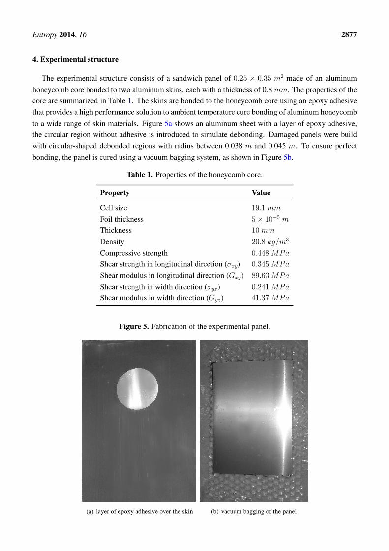
The experimental structure consists of a sandwich panel of 0.25 × 0.35 m2 made of an aluminumhoneycomb core bonded to two aluminum skins, each with a thickness of 0.8 mm. The properties of thecore are summarized in Table 1. The skins are bonded to the honeycomb core using an epoxy adhesivethat provides a high performance solution to ambient temperature cure bonding of aluminum honeycombto a wide range of skin materials. Figure 5a shows an aluminum sheet with a layer of epoxy adhesive,the circular region without adhesive is introduced to simulate debonding. Damaged panels were buildwith circular-shaped debonded regions with radius between 0.038 m and 0.045 m. To ensure perfectbonding, the panel is cured using a vacuum bagging system, as shown in Figure 5b.

Table 1. Properties of the honeycomb core.

Property Value

Cell size 19.1mm

Foil thickness 5× 10−5 m

Thickness 10mm

Density 20.8 kg/m3

Compressive strength 0.448MPa

Shear strength in longitudinal direction (σxy) 0.345MPa

Shear modulus in longitudinal direction (Gxy) 89.63MPa

Shear strength in width direction (σyz) 0.241MPa

Shear modulus in width direction (Gyz) 41.37MPa

Figure 5. Fabrication of the experimental panel.

(a) layer of epoxy adhesive over the skin (b) vacuum bagging of the panel

Entropy 2014, 16 2878

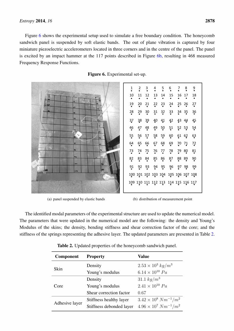
Figure 6 shows the experimental setup used to simulate a free boundary condition. The honeycombsandwich panel is suspended by soft elastic bands. The out of plane vibration is captured by fourminiature piezoelectric accelerometers located in three corners and in the centre of the panel. The panelis excited by an impact hammer at the 117 points described in Figure 6b, resulting in 468 measuredFrequency Response Functions.

Figure 6. Experimental set-up.

(a) panel suspended by elastic bands

1 2 3 4 5 6 7 8 9

10 11 12 13 14 15 16 17 18

19 20 21 22 23 24 25 26 27

28 29 30 31 32 33 34 35 36

37 38 39 40 41 42 43 44 45

46 47 48 49 50 51 52 53 54

55 56 57 58 59 60 61 62 63

64 65 66 67 68 69 70 71 72

73 74 75 76 77 78 79 80 81

82 83 84 85 86 87 88 89 90

91 92 93 94 95 96 97 98 99

100 101 102 103 104 105 106 107 108

109 110 111 112 113 114 115 116 117

(b) distribution of measurement point

The identified modal parameters of the experimental structure are used to update the numerical model.The parameters that were updated in the numerical model are the following: the density and Young’sModulus of the skins; the density, bending stiffness and shear correction factor of the core; and thestiffness of the springs representing the adhesive layer. The updated parameters are presented in Table 2.

Table 2. Updated properties of the honeycomb sandwich panel.

Component Property Value

SkinDensity 2.53× 103 kg/m3

Young’s modulus 6.14× 1010 Pa

CoreDensity 31.1 kg/m3

Young’s modulus 2.41× 1010 Pa

Shear correction factor 0.67

Adhesive layerStiffness healthy layer 3.42× 108 Nm−1/m2

Stiffness debonded layer 4.96× 107 Nm−1/m2

Entropy 2014, 16 2879

Figure 7 shows the first six experimental mode shapes compared to those from the numerical modelafter updating. The correlation between two mode shapes is measured by the Modal Assurance Criterion(MAC), defined as,

MACi =

(φT

N,iφE,i

)2(φT

N,iφN,i

) (φT

E,iφE,i

) (11)

Where φi is the ith mode shape, subscripts N , E refer to numerical and experimental respectively. AMAC value of 0 indicates no correlation whereas a value of 1 indicates two completely correlated modes.

The results show that the correlation between the numerical and experimental modes is almost perfectfor the first three modes, with MAC values higher than 0.99. The fifth mode presents the lowestcorrelation, with a MAC value of 0.83. In this case, the first-order shear approximation may not besufficient. The maximum difference between the experimental and the numerical natural frequenciesis 11%.

Figure 8 presents the correlation between the numerical and experimental global modes for the casewith a circular debonded region at the centre of the plate. The modes are plotted over the surface ofthe debonded skin. Here, the numerical model was updated again considering the spring stiffness in thedebonded region as updating parameter. Although the correlation is not as good as in the undamagedcase, both the numerical and experimental models show the same behavior in the presence of damage,which is a reduction in the natural frequencies, and a strong discontinuity at the debonded regionfor mode 4.

Figure 7. Numerical and experimental undamaged mode shapes.

n=520.9, e=483.1, MAC=0.998

Numerical Experimental

n=600.8, e=621.0, MAC=0.994


n=1089.5, e=986.7, MAC=0.995


n=1105.1, e=1214.6, MAC=0.984


n=1406.8, e=1377.0, MAC=0.831


n=1598.5, e=1528.9, MAC=0.967


Entropy 2014, 16 2880

Figure 8. Numerical and experimental mode shapes with a debonded region at the center ofthe panel.

n=520.9, e=477.4, MAC=0.998


n=598.8, e=618.2, MAC=0.993


n=1088.8, e=947.2, MAC=0.975


n=1029.4, e=1158.4, MAC=0.841


n=1276.4, e=1306.9, MAC=0.698


n=1598.3, e=1505.7, MAC=0.989


5. Construction of the Database

The database is built as follows:

(1) Define a set of damage scenarios to be used in the database.

(2) Set j = 1.

(3) Parameterized the jth scenario with an observation vector Yj .

(4) Build the numerical model associated with the jth scenario.

(5) Construct a feature vector Xj using the modal parameters derived from the numerical model.

(6) Add the pair of vectors (Xj,Yj) to the database, set j = j + 1 and go to step 3.

The damage scenarios used to construct the database consist of panels with circular-shaped debondedregions at one of the 117 points that are depicted in Figure 6b. Debonding is restricted to the skin thatis measured during experiments. For each of the 117 points, thirteen debonded radius between 0.01 mand 0.07 m are considered (i.e. 0.01, 0.015, . . . , 0.065, 0.07) resulting in 1521 pairs of vectors in thedatabase. The next subsections describe how the observation and feature vectors are built.

Entropy 2014, 16 2881

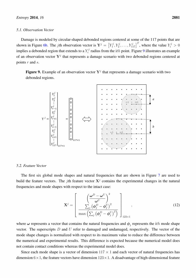
5.1. Observation Vector

Damage is modeled by circular-shaped debonded regions centered at some of the 117 points that areshown in Figure 6b. The jth observation vector is Yj =

[Y j1 , Y

j2 , . . . , Y

j117

]T, where the value Y j

i > 0

implies a debonded region that extends to a Y ji radius from the ith point. Figure 9 illustrates an example

of an observation vector Yj that represents a damage scenario with two debonded regions centered atpoints r and s.

Figure 9. Example of an observation vector Yj that represents a damage scenario with twodebonded regions.

Y

⋮

⋮

⋮

00⋮0

0⋮0

0⋮0

r‐1 r r+1a

s‐1 s s+1

b

5.2. Feature Vector

The first six global mode shapes and natural frequencies that are shown in Figure 7 are used tobuild the feature vectors. The jth feature vector Xj contains the experimental changes in the naturalfrequencies and mode shapes with respect to the intact case:

Xj =

(ωD − ωU

ωU

)2

∑j

(φD

j − φUj

)2max

(∑j

(φD

j − φUj

)2)

123×1

, (12)

where ω represents a vector that contains the natural frequencies and φj represents the ith mode shapevector. The superscripts D and U refer to damaged and undamaged, respectively. The vector of themode shape changes is normalized with respect to its maximum value to reduce the difference betweenthe numerical and experimental results. This difference is expected because the numerical model doesnot contain contact conditions whereas the experimental model does.

Since each mode shape is a vector of dimension 117 × 1 and each vector of natural frequencies hasdimension 6×1, the feature vectors have dimension 123×1. A disadvantage of high-dimensional feature

Entropy 2014, 16 2882

spaces, as the present case, is that points that are scattered in those spaces are usually far from eachother. Thus, neighborhood methods that are based purely on distance become less useful. Nevertheless,Gupta [26] showed that the linear approximation with maximum entropy is more suited than standardneighborhood methods for three and higher dimension feature spaces.

6. Damage Assessment Results

The algorithm is tested for the three experimental damage scenarios shown in Figure 10. The firstcase has a debonded region centered at point 59 (the centre of the panel), the second case has a debondedregion centered nearby points 30, 31, 39 and 40, and the third case has a debonded region centerednearby points 31, 32, 40, 41. The radius for the three debonded regions are 0.038 m, 0.039 m and 0.045m respectively. Debonding was introduced into the experimental panels by purposely leaving circularareas without adhesive as shown in Figure 5a.

Figure 10. Experimental damage scenarios introduced to the panel; debonded regions areenclosed by circles.

1 2 3 4 5 6 7 8 9

10 11 12 13 14 15 16 17 18

19 20 21 22 23 24 25 26 27

28 29 30 31 32 33 34 35 36

37 38 39 40 41 42 43 44 45

46 47 48 49 50 51 52 53 54

55 56 57 58 59 60 61 62 63

64 65 66 67 68 69 70 71 72

73 74 75 76 77 78 79 80 81

82 83 84 85 86 87 88 89 90

91 92 93 94 95 96 97 98 99

100 101 102 103 104 105 106 107 108

109 110 111 112 113 114 115 116 117

1 2 3 4 5 6 7 8 9

10 11 12 13 14 15 16 17 18

19 20 21 22 23 24 25 26 27

28 29 30 31 32 33 34 35 36

37 38 39 40 41 42 43 44 45

46 47 48 49 50 51 52 53 54

55 56 57 58 59 60 61 62 63

64 65 66 67 68 69 70 71 72

73 74 75 76 77 78 79 80 81

82 83 84 85 86 87 88 89 90

91 92 93 94 95 96 97 98 99

100 101 102 103 104 105 106 107 108

109 110 111 112 113 114 115 116 117

1 2 3 4 5 6 7 8 9

10 11 12 13 14 15 16 17 18

19 20 21 22 23 24 25 26 27

28 29 30 31 32 33 34 35 36

37 38 39 40 41 42 43 44 45

46 47 48 49 50 51 52 53 54

55 56 57 58 59 60 61 62 63

64 65 66 67 68 69 70 71 72

73 74 75 76 77 78 79 80 81

82 83 84 85 86 87 88 89 90

91 92 93 94 95 96 97 98 99

100 101 102 103 104 105 106 107 108

109 110 111 112 113 114 115 116 117

a) b) c)(a)

1 2 3 4 5 6 7 8 9

10 11 12 13 14 15 16 17 18

19 20 21 22 23 24 25 26 27

28 29 30 31 32 33 34 35 36

37 38 39 40 41 42 43 44 45

46 47 48 49 50 51 52 53 54

55 56 57 58 59 60 61 62 63

64 65 66 67 68 69 70 71 72

73 74 75 76 77 78 79 80 81

82 83 84 85 86 87 88 89 90

91 92 93 94 95 96 97 98 99

100 101 102 103 104 105 106 107 108

109 110 111 112 113 114 115 116 117

1 2 3 4 5 6 7 8 9

10 11 12 13 14 15 16 17 18

19 20 21 22 23 24 25 26 27

28 29 30 31 32 33 34 35 36

37 38 39 40 41 42 43 44 45

46 47 48 49 50 51 52 53 54

55 56 57 58 59 60 61 62 63

64 65 66 67 68 69 70 71 72

73 74 75 76 77 78 79 80 81

82 83 84 85 86 87 88 89 90

91 92 93 94 95 96 97 98 99

100 101 102 103 104 105 106 107 108

109 110 111 112 113 114 115 116 117

1 2 3 4 5 6 7 8 9

10 11 12 13 14 15 16 17 18

19 20 21 22 23 24 25 26 27

28 29 30 31 32 33 34 35 36

37 38 39 40 41 42 43 44 45

46 47 48 49 50 51 52 53 54

55 56 57 58 59 60 61 62 63

64 65 66 67 68 69 70 71 72

73 74 75 76 77 78 79 80 81

82 83 84 85 86 87 88 89 90

91 92 93 94 95 96 97 98 99

100 101 102 103 104 105 106 107 108

109 110 111 112 113 114 115 116 117

a) b) c)(b)

1 2 3 4 5 6 7 8 9

10 11 12 13 14 15 16 17 18

19 20 21 22 23 24 25 26 27

28 29 30 31 32 33 34 35 36

37 38 39 40 41 42 43 44 45

46 47 48 49 50 51 52 53 54

55 56 57 58 59 60 61 62 63

64 65 66 67 68 69 70 71 72

73 74 75 76 77 78 79 80 81

82 83 84 85 86 87 88 89 90

91 92 93 94 95 96 97 98 99

100 101 102 103 104 105 106 107 108

109 110 111 112 113 114 115 116 117

1 2 3 4 5 6 7 8 9

10 11 12 13 14 15 16 17 18

19 20 21 22 23 24 25 26 27

28 29 30 31 32 33 34 35 36

37 38 39 40 41 42 43 44 45

46 47 48 49 50 51 52 53 54

55 56 57 58 59 60 61 62 63

64 65 66 67 68 69 70 71 72

73 74 75 76 77 78 79 80 81

82 83 84 85 86 87 88 89 90

91 92 93 94 95 96 97 98 99

100 101 102 103 104 105 106 107 108

109 110 111 112 113 114 115 116 117

1 2 3 4 5 6 7 8 9

10 11 12 13 14 15 16 17 18

19 20 21 22 23 24 25 26 27

28 29 30 31 32 33 34 35 36

37 38 39 40 41 42 43 44 45

46 47 48 49 50 51 52 53 54

55 56 57 58 59 60 61 62 63

64 65 66 67 68 69 70 71 72

73 74 75 76 77 78 79 80 81

82 83 84 85 86 87 88 89 90

91 92 93 94 95 96 97 98 99

100 101 102 103 104 105 106 107 108

109 110 111 112 113 114 115 116 117

a) b) c)(c)

The results of the max-ent linear approximation algorithm are compared with those obtained bysolving the nonnegative least-squares problem posed in Equation (2). The procedure to assess theexperimental damage using both approaches is implemented as follows:

(1) Perform an experimental modal analysis of the damaged panel and identify the first six globalmode shapes and natural frequencies.

(2) Construct the feature test point X using Equation (12).

(3) Read the feature vectors in the database.

(4) Compute weights.

Entropy 2014, 16 2883

Max-ent

(a) Select parameter βi in the Gaussian prior given in Equation (7), so that k neighbors contributeto the solution.

(b) Solve the system of nonlinear equations presented in Equation (10).

(c) Compute the weight functions from Equation (8).

Nonnegative least-squares

(a) Select the k closest neighbors.

(b) Build the matrices A and b in Equation (2).

(c) Compute the weights using the Matlab function lsqnonneg.

(5) Read the observation vectors in the database and estimate the experimental damage from (3).

Both methods use the ten closest neighbors to the test point. The time needed to solve the linearapproximation problem (stages 4 and 5 above) is 0.7 and 0.03 seconds for the max-ent and nonnegativeleast-squares approaches, respectively. Table 3 details the running time of both algorithms. It is clearthat a more efficient method to select the parameter βi could greatly reduce the computational time ofthe max-ent approach. Nevertheless, it should be noted that both algorithms can reach a solution in lessthan a second, which can be considered real-time for structural damage assessment problems. Otheralgorithms such as parallel genetic algorithms can take between 1000 and 10000 seconds to solve asimilar problem [12].

Table 3. Running time for each stage of the linear approximation method.

Stage Time (s)Max-ent Nonnegative least-squares

4 (a) 5.91×10−1 4.30×10−3

(b) 9.89×10−2 1.24×10−4

(c) 1.00×10−2 2.90×10−3

5 8.7×10−5 8.7×10−5

Figures 11, 12 and 13 present the damage assessment results. In these figures, the black zones indicatethe detected damage, where each pixel represents a debonded spring. The actual damage introduced intothe panel is depicted by a circle. In the three cases, the max-ent approach identifies debonded regionsthat are closer to the actual damage than those identified by the least-squares method. In the first case,the centre of the experimental damage matches one of the 117 predefined locations. Thus, the max-entalgorithm is able to detect the exact location of the debonded region. However, when the actual centreof the damage does not match one of the 117 locations, as in the second and third cases, the algorithmdetects the damage at a location that is close to the actual location but not at the exact location.

Entropy 2014, 16 2884

Figure 11. Damage assessment results for the first damage scenario.

(a) Max-ent (b) Nonnegative least-squares

Figure 12. Damage assessment results for the second damage scenario.


Entropy 2014, 16 2885

Figure 13. Damage assessment results for the third damage scenario.


7. Conclusions and Further Research

This article presented a new methodology to identify debonded regions in aluminum honeycombpanels using a linear approximation method handled by a statistical inference model based on themaximum-entropy principle. The algorithm was validated using experimental data from an aluminumhoneycomb panel subjected to different damage scenarios.

The honeycomb panels were modeled with finite elements using a simplified three-layer shell model.The adhesive layer between the skin and core was modeled using linear springs with the rigidity beingreduced at debonded locations. This numerical model predicted the first six modes of the undamagedand damaged panels with reasonable accuracy. Nevertheless, the numerical model can be improved byusing higher order shear approximations.

In the three experimental cases, the linear approximation using the max-ent technique was successfulin assessing the experimental damage. The detected damage closely corresponds with the experimentaldamage in all cases. In addition, the damage state of the panels is assessed in less than one secondthereby providing the possibility of real-time damage assessment.

The results show that the proposed algorithm can assess debonded regions with sizes between 0.038m and 0.045 m. It would be useful to establish the minimum size that can be detected with confidence.This value largely depends on the sensitivity of mode shapes and natural frequencies to damage and onthe level of experimental variability.

Entropy 2014, 16 2886

The proposed damage assessment algorithm provides only two options for a spring in the adhesivelayer: either healthy or debonded. This can be improved by setting the output for each spring as a numberassociated with a debonding probability that ranges from 0 to 1.

Lastly, further research is needed to adapt this algorithm to cases with multiple debonded regions andto test its performance in more realistic configurations than a free plate.

Acknowledgments

Valentina del Fierro was supported by CONICYT grant CONICYT-PCHA/Magï£¡sterNacional/2013-221320691. The authors acknowledge the partial financial support of the ChileanNational Fund for Scientific and Technological Development (Fondecyt) under Grants No. 11110389and 11110046.

Author Contributions

Viviana Meruane and Valentina del Fierro built the updated numerical model, designed theexperiment, processed and analyzed the experimental data, and tested the damage assessment algorithm.Alejandro Ortiz-Bernardin programmed the max-ent linear approximation algorithm and adapted it tothe application case. The article was written by Viviana Meruane and Alejandro Ortiz-Bernardin.

Conflicts of Interest

The authors declare no conflict of interest

References

1. Vinson, J.R. Sandwich structures: past, present, and future. In Sandwich Structures 7: Advancingwith Sandwich Structures and Materials; Springer: Dordrecht, The Netherlands, 2005; pp. 3–12.

2. Carden, E.; Fanning, P. Vibration Based Condition Monitoring: A Review. Struct. Health Monit.2004, 3, 355–377.

3. Zou, Y.; Tong, L.; Steven, G. Vibration-based model-dependent damage (delamination)identification and health monitoring for composite structures-a review. J. Sound Vib. 2000,230, 357–378.

4. Montalvao, D.; Maia, N.; Ribeiro, A. A Review of Vibration-based Structural Health Monitoringwith Special Emphasis on Composite Materials. Shock Vib. Digest 2006, 38, 295–324.

5. Jiang, L.; Liew, K.; Lim, M.; Low, S. Vibratory behaviour of delaminated honeycomb structures:A 3-D finite element modelling. Comput. Struct. 1995, 55, 773–788.

6. Kim, H.Y.; Hwang, W. Effect of debonding on natural frequencies and frequency responsefunctions of honeycomb sandwich beams. Compos. Struct. 2002, 55, 51–62.

7. Burlayenko, V.; Sadowski, T. Dynamic behaviour of sandwich plates containing single/multipledebonding. Comput. Mater. Sci. 2011, 50, 1263–1268.

Entropy 2014, 16 2887

8. Burlayenko, V.N.; Sadowski, T. Influence of skin/core debonding on free vibration behavior offoam and honeycomb cored sandwich plates. Int. J. Non-Lin. Mech. 2010, 45, 959–968.

9. Mohanan, A.; Pradeep, K.; Narayanan, K. Performance Assessment of Sandwich Structures withDebonds and Dents. Int. J. Sci. Eng. Res. 2013, 4, 174–179.

10. Shahdin, A.; Morlier, J.; Gourinat, Y. Damage monitoring in sandwich beams by modalparameter shifts: A comparative study of burst random and sine dwell vibration testing.J. Sound Vib. 2010, 329, 566–584.

11. Farrar, C.; Lieven, N. Damage prognosis: the future of structural health monitoring. Philos.Trans. A Math. Phys. Eng. Sci. 2007, 365, 623–632.

12. Meruane, V.; Heylen, W. Damage detection with parallel genetic algorithms and operationalmodes. Struct. Health Monit. 2010, 9, 481–496.

13. Meruane, V.; Heylen, W. An hybrid real genetic algorithm to detect structural damage usingmodal properties. Mech. Syst. Signal Process. 2011, 25, 1559–1573.

14. Perera, R.; Torres, R. Structural damage detection via modal data with genetic algorithms.J. Struct. Eng. 2006, 132, 1491–1501.

15. Kouchmeshky, B.; Aquino, W.; Bongard, J.; Lipson, H. Co-evolutionary algorithm for structuraldamage identification using minimal physical testing. Int. J. Numer. Meth. Eng. 2007,69, 1085–1107.

16. Teughels, A.; De Roeck, G.; Suykens, J. Global optimization by coupled local minimizers andits application to FE model updating. Comput. Struct. 2003, 81, 2337–2351.

17. Markou, M.; Singh, S. Novelty detection: a review–part 1: statistical approaches. Signal Process.2003, 83, 2481–2497.

18. Islam, A.S.; Craig, K.C. Damage detection in composite structures using piezoelectric materials(and neural net). Smart Mater. Struct. 1994, 3, 318–328.

19. Okafor, A.C.; Chandrashekhara, K.; Jiang, Y. Delamination prediction in composite beams withbuilt-in piezoelectric devices using modal analysis and neural network. Smart Mater. Struct.1996, 5, 338–347.

20. Valoor, M.T.; Chandrashekhara, K. A thick composite-beam model for delamination predictionby the use of neural networks. Compos. Sci. Tech. 2000, 60, 1773–1779.

21. Ishak, S.; Liu, G.; Shang, H.; Lim, S. Locating and sizing of delamination in composite laminatesusing computational and experimental methods. Compos. B Eng. 2001, 32, 287–298.

22. Chakraborty, D. Artificial neural network based delamination prediction in laminated composites.Mater. Des. 2005, 26, 1–7.

23. Su, Z.; Ling, H.Y.; Zhou, L.M.; Lau, K.T.; Ye, L. Efficiency of genetic algorithms and artificialneural networks for evaluating delamination in composite structures using fibre Bragg gratingsensors. Smart Mater. Struct. 2005, 14, 1541–1553.

24. Zhang, Z.; Shankar, K.; Ray, T.; Morozov, E.V.; Tahtali, M. Vibration-Based Inverse Algorithmsfor Detection of Delamination in Composites. Compos. Struct. 2013, 102, 226–236.

25. Meruane, V.; Mahu, J. Real-time structural damage assessment using artificial neural networksand anti-resonant frequencies. Shock Vib. 2014, 2014, 653279:1–653279:14.

Entropy 2014, 16 2888

26. Gupta, M.R. An information theory approach to supervised learning. PhD thesis, StanfordUniversity, CA, USA, 2003.

27. Gupta, M.R.; Gray, R.M.; Olshen, R.A. Nonparametric supervised learning by linearinterpolation with maximum entropy. IEEE Trans. Pattern Anal. Mach. Intell. 2006,28, 766–781.

28. Jaynes, E.T. Information theory and statistical mechanics. Phys. Rev. 1957, 106, 620–630.29. Erkan, A.N. Semi-supervised learning via generalized maximum entropy. PhD thesis, New York

University, NY, USA, 2010.30. Lawson, C.L.; Hanson, R.J. Solving least squares problems; SIAM: New Jersey, USA, 1974;

pp. 161–164.31. Arroyo, M.; Ortiz, M. Local maximum-entropy approximation schemes: A seamless bridge

between finite elements and meshfree methods. Int. J. Numer. Meth. Eng. 2006, 65, 2167–2202.32. Ortiz, A.; Puso, M.A.; Sukumar, N. Maximum-entropy meshfree method for compressible and

near-incompressible elasticity. Comput. Meth. Appl. Mech. Eng. 2010, 199, 1859–1871.33. Yaw, L.L.; Sukumar, N.; Kunnath, S.K. Meshfree co-rotational formulation for two-dimensional

continua. Int. J. Numer. Meth. Eng. 2009, 79, 979–1003.34. Cyron, C.J.; Arroyo, M.; Ortiz, M. Smooth, second order, non-negative meshfree approximants

selected by maximum entropy. Int. J. Numer. Meth. Eng. 2009, 79, 1605–1632.35. Rosolen, A.M.; Millán, R.D.; Arroyo, M. On the optimum support size in meshfree methods: A

variational adaptivity approach with maximum entropy approximants. Int. J. Numer. Meth. Eng.2010, 82, 868–895.

36. González, D.; Cueto, E.; Doblaré, M. A higher order method based on local maximum entropyapproximation. Int. J. Numer. Meth. Eng. 2010, 83, 741–764.

37. Li, B.; Habbal, F.; Ortiz, M. Optimal transportation meshfree approximation schemes for fluidand plastic flows. Int. J. Numer. Meth. Eng. 2010, 83, 1541–1579.

38. Cyron, C.; Nissen, K.; Gravemeier, V.; Wall, W. Stable meshfree methods in fluid mechanicsbased on Green’s functions. Comput. Mech. 2010, 46, 287–300.

39. Cyron, C.; Nissen, K.; Gravemeier, V.; Wall, W. Information flux maximum-entropyapproximation schemes for convection and diffusion problems. Int. J. Numer. Meth. Fluid.2010, 64, 1180–1200.

40. Gamboa, F.; Gassiat, E. Bayesian methods and maximum entropy for ill-posed inverse problems.Ann. Stat. 1997, 25, 328–350.

41. Loubes, J.M.; Pelletier, B. Maximum entropy solution to ill-posed inverse problems withapproximately known operator. J. Math. Anal. Appl 2008, 344, 260–273.

42. Shannon, C.E. A mathematical theory of communication. Bell Syst. Tech. J. 1948, 27, 379–423.43. Sukumar, N.; Wright, R.W. Overview and construction of meshfree basis functions: From

moving least squares to entropy approximants. Int. J. Numer. Meth. Eng. 2007, 70, 181–205.44. Kullback, S. Information Theory and Statistics; Wiley: New York, USA, 1959.45. Shore, J.E.; Johnson, R.W. Axiomatic derivation of the principle of maximum entropy and the

principle of minimum cross-entropy. IEEE Trans. Inform. Theor. 1980, 26, 26–36.

Entropy 2014, 16 2889

46. Burton, W.S.; Noor, A.K. Assessment of computational models for sandwich panels and shells.Comput. Meth. Appl. Mech. Eng. 1995, 124, 125–151.

47. Birman, V.; Bert, C.W. On the choice of shear correction factor in sandwich structures. J. Sandw.Struct. and Mater. 2002, 4, 83–95.

48. Burton, W.; Noor, A. Assessment of continuum models for sandwich panel honeycomb cores.Comput. Meth. Appl. Mech. Eng. 1997, 145, 341–360.

49. Tanimoto, Y.; Nishiwaki, T.; Shiomi, T.; Maekawa, Z. A numerical modeling for eigenvibrationanalysis of honeycomb sandwich panels. Compos. Interfac. 2001, 8, 393–402.

50. Burlayenko, V.N.; Sadowski, T. Analysis of structural performance of sandwich plates withfoam-filled aluminum hexagonal honeycomb core. Comput. Mater. Sci. 2009, 45, 658–662.

51. Della, C.N.; Shu, D. Vibration of delaminated composite laminates: A review. Appl. Mech. Rev.2007, 60, 1–20.

52. Müller, I. Clapping in delaminated sandwich-beams due to forced oscillations. Comput. Mech.2007, 39, 113–126.

53. SDTools. Structural dynamics toolbox & FEMLink. Users Guide Version; SDTools: Paris,France, 2014.

c© 2014 by the authors; licensee MDPI, Basel, Switzerland. This article is an open access articledistributed under the terms and conditions of the Creative Commons Attribution license(http://creativecommons.org/licenses/by/3.0/).

Documents

OPEN ACCESS entropy