Onshore Lower 48 Oil and Gas Supply Submodule Coponent ... · PDF fileStatement of Purpose ... Summary of Models Reviewed ... Onshore Lower 48 Oil and Gas Supply Submodule Coponent

Onshore Lower 48 Oil and Gas Supply

Submodule

Component Design Report

December 2006

Prepared for: Office of Integrated Analysis and Forecasting

Energy Information Administration U.S. Department of Energy

Work Performed Under: Prime Contract Number DE-AM01-04EI42006

Task Order# DE-AT01-05EI40220.A000 &

Task Order# DE-AT01-06EI40242.A000

Prepared By: INTEK Incorporated

Resource Consultants, Inc.

INTEK

Onshore Lower 48 Oil and Gas Supply Submodule

Component Design Report

December 2006

Prepared for: Office of Integrated Analysis and Forecasting

Energy Information Administration U.S. Department of Energy

Work Performed Under: Prime Contract Number DE-AM01-04EI42006

Task Order# DE-AT01-05EI40220.A000 &

Task Order# DE-AT01-06EI40242.A000

Prepared By: INTEK Incorporated

Resource Consultants, Inc.

INTEK

Disclaimer

This report was prepared as an account of work sponsored by an agency of the United States Government. Neither the United States Government nor any agency thereof, nor any of their employees or contractors, makes any warranty, express or implied, or assumes any legal liability or responsibility for the accuracy, completeness, or usefulness of any information, apparatus, product, or process disclosed, or represents that its use would not infringe privately owned rights. Reference herein to any specific commercial product, process or service by trade name, trademark, manufacture, or otherwise, does not necessarily constitute or imply its endorsement, recommendation, or favoring by the United States Government or any agency thereof. The views and opinions of authors expressed herein do not necessarily state or reflect those of the United States Government or any agency thereof.

Energy Information Administration Component Design Report – Onshore Lower 48 Oil and Gas Supply Submodule iv

Table of Contents

1. Executive Summary...................................................................................................... 1 2. Statement of Purpose.................................................................................................... 2

2.1. Resources Modeled............................................................................................. 3 2.1.1. Oil Resources .............................................................................................. 3 2.1.2. Natural Gas Resources................................................................................ 4

2.2. Major Enhancements of Proposed OLOGSS...................................................... 5 3. Background Research................................................................................................... 6

3.1. Types of Oil and Gas Models ............................................................................. 6 3.1.1. Geologic/Engineering ................................................................................. 6 3.1.2. Econometric ................................................................................................ 6 3.1.3. Hybrid ......................................................................................................... 6

3.2. Oil and Gas Supply Models/Methodologies Considered.................................... 7 4. Input/ Output Requirements ....................................................................................... 9

4.1. Unit of Analysis .................................................................................................. 9 4.1.1. Bin Classification...................................................................................... 10

4.2. Types of Data.................................................................................................... 10 4.3. Resource Data ................................................................................................... 11

4.3.1. Resource Data for Discovered Resource .................................................. 11 4.3.2. Resource Data for Undiscovered Resource .............................................. 12

4.4. Production Data ................................................................................................ 14 4.5. Cost Data........................................................................................................... 15

4.5.1. Capital Costs ............................................................................................. 16 4.5.2. Operating Costs......................................................................................... 20 4.5.3. Other Cost Parameters .............................................................................. 23

4.6. Development Constraint Data........................................................................... 24 4.6.1. Capital Constraints.................................................................................... 26 4.6.2. Other Development Constraints................................................................ 26

5. Classification Plan....................................................................................................... 28 5.1. Definition of Regions........................................................................................ 28

6. Methodology Description ........................................................................................... 30 6.1. Model Objective................................................................................................ 30 6.2. Model Structure ................................................................................................ 30

6.2.1. Master Database........................................................................................ 31 6.2.2. Resource Description Module................................................................... 32 6.2.3. Process Module......................................................................................... 36 6.2.4. Economic/ Timing Module ....................................................................... 38 6.2.5. Modeling Impact of Technology Improvement........................................ 51 6.2.6. Reporting Module ..................................................................................... 58

7. Uncertainty and Limitations...................................................................................... 60 7.1. Assumptions...................................................................................................... 60 7.2. Limitation of Model.......................................................................................... 60

8. Conclusions and Recommendations.......................................................................... 62 8.1. Conclusions....................................................................................................... 62

Energy Information Administration Component Design Report – Onshore Lower 48 Oil and Gas Supply Submodule v

8.2. Recommendations............................................................................................. 62 9. References.................................................................................................................... 63

Energy Information Administration Component Design Report – Onshore Lower 48 Oil and Gas Supply Submodule vi

List of Figures

Figure 2.1: Relationships among NEMS, OGSM, PMM, and NGTDM............................ 2 Figure 2.2: Subcomponents within OGSM......................................................................... 3 Figure 2.3: Crude Oil Resource .......................................................................................... 4 Figure 2.4: Natural Gas Resource....................................................................................... 4 Figure 4.1: Bin Classification for Size and Depth ............................................................ 10 Figure 4.2: Types of Data Required by OLOGSS ............................................................ 11 Figure 4.3: Cost Data Requirements................................................................................. 15 Figure 4.4: Relationship Between Oil Price and Available Drilling Footage................... 25 Figure 5.1: Onshore Lower 48 Oil and Gas Supply Submodule Regions ........................ 28 Figure 6.1: OLOGSS System Logic Flow ........................................................................ 31 Figure 6.2: Resource Description Module Flowchart....................................................... 32 Figure 6.3: Hypothetical Decline Curves for Three Wells ............................................... 34 Figure 6.4: Example of Process Specific Type Curve ...................................................... 36 Figure 6.5: Timing/ Economic Module Flowchart ........................................................... 40 Figure 6.6: Example of Bin Population Methodology...................................................... 42 Figure 6.7: Exploration Flowchart.................................................................................... 43 Figure 6.8: Logic Flow of Cashflow Procedure................................................................ 46 Figure 6.9: Production Decline Flowchart........................................................................ 46 Figure 6.10: Ranking and Selection Logic Flow .............................................................. 49 Figure 6.11: Impact of Economic and Technology Levers............................................... 52 Figure 6.12: Generic Technology Penetration Curve ....................................................... 53 Figure 6.13: Potential Market Penetration Profiles........................................................... 54 Figure 6.14: Technology Penetration Curve for New Drill Bit ........................................ 57

Energy Information Administration Component Design Report – Onshore Lower 48 Oil and Gas Supply Submodule vii

List of Tables

Table 3.1: Summary of Models Reviewed ......................................................................... 7 Table 4.1: Resource Data Categories................................................................................ 12 Table 4.2: Size Class Definitions for Undiscovered Conventional Accumulations ......... 13 Table 4.3: Size Class Definitions for Undiscovered Unconventional Accumulations ..... 14 Table 4.4: Capital and Operating Costs for Oil Processes................................................ 15 Table 4.5: Capital and Operating Costs for Gas Processes............................................... 16 Table 4.6: Regional Cost Ratios for Secondary Production Operating Costs .................. 21 Table 4.7: Injectant Costs for EOR and ASR Processes................................................... 22 Table 5.1: Onshore Lower 48 Oil and Gas Supply Submodule Regions.......................... 29 Table 6.1: Sources of Resource Data................................................................................ 32 Table 6.2: Corresponding Well Bin Population................................................................ 34 Table 6.3: Process Specific Technology Levers for Oil ................................................... 38

Energy Information Administration Component Design Report – Onshore Lower 48 Oil and Gas Supply Submodule viii

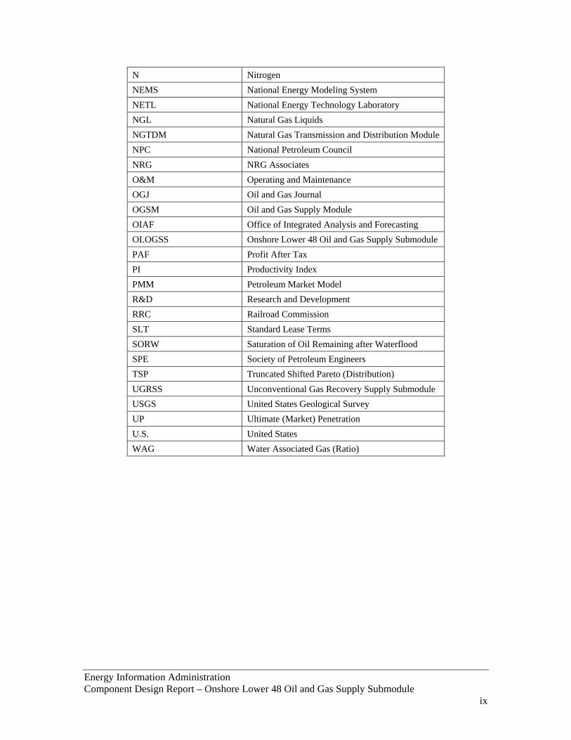
List of Abbreviations This table lists the abbreviations and acronyms used in the “Onshore Lower 48 Oil and Gas Supply Submodule Component Design Report”.

Abbreviation/ Acronym Full Text API American Petroleum Institute ASR Advanced Secondary Recovery BBL Barrel BLM Bureau of Land Management BOE Barrel of Oil Equivalent BOEPD Barrel of Oil Equivalent Per Day COGAM Comprehensive Oil and Gas Analysis Model CO2 Carbon Dioxide DFO EIA Dallas Field Office D&C Drilling and Completion DOE Department of Energy EIA Energy Information Administration EOR Enhanced Oil Recovery EPCA Energy Policy and Conservation Act EUR Estimated Ultimate Recovery FT Foot G&G Geological and Geophysical GOR Gas Oil Ratio GTI Gas Technology Institute H2S Hydrogen Sulfide HPDI HPDI Production Data IHS IHS Energy IOR Improved Oil Recovery IPAA Independent Petroleum Association of America IRS Internal Revenue Service JAS “Joint Annual Survey on Drilling Costs” K$ Thousand Dollars Lb Pound MBbl Thousand Barrels MCF Thousand Cubic Feet MMCF Million Cubic Feet MMBBL Million Barrel MMBOE Million Barrels of Oil Equivalent MMS Minerals Management Service

Energy Information Administration Component Design Report – Onshore Lower 48 Oil and Gas Supply Submodule ix

N Nitrogen NEMS National Energy Modeling System NETL National Energy Technology Laboratory NGL Natural Gas Liquids NGTDM Natural Gas Transmission and Distribution Module NPC National Petroleum Council NRG NRG Associates O&M Operating and Maintenance OGJ Oil and Gas Journal OGSM Oil and Gas Supply Module OIAF Office of Integrated Analysis and Forecasting OLOGSS Onshore Lower 48 Oil and Gas Supply Submodule PAF Profit After Tax PI Productivity Index PMM Petroleum Market Model R&D Research and Development RRC Railroad Commission SLT Standard Lease Terms SORW Saturation of Oil Remaining after Waterflood SPE Society of Petroleum Engineers TSP Truncated Shifted Pareto (Distribution) UGRSS Unconventional Gas Recovery Supply Submodule USGS United States Geological Survey UP Ultimate (Market) Penetration U.S. United States WAG Water Associated Gas (Ratio)

1. Executive Summary The United States has long recognized the importance of developing accurate mid-term forecasts of the oil and gas production from the United States. As such, the Office of Integrated Analysis and Forecasting (OIAF) was tasked at its inception to construct a set of fully integrated mid-term energy models to function as the National Energy Modeling System (NEMS). Within NEMS, the Oil and Gas Supply Module (OGSM) represents the regional domestic crude and natural gas production and all natural gas imports. Since the original development of the OGSM, several major steps have been taken to improve the model’s capabilities, including: • Regular review and enhancement of the OGSM submodules.

• The incorporation of the Unconventional Gas Recovery Supply Submodule.

• Most recently, the DOE/EIA sought to review and redevelop the methodology used to forecast domestic crude and natural gas production from the Onshore Lower 48. The results of this initiative are presented in this report.

The new OLOGSS submodule relies on publicly available information. The design incorporates the best features of the existing models available from both private and public sources. This model incorporates a resource database containing detailed petrochemical and geologic data on discovered and undiscovered resources in the Lower 48 onshore. An engineering-based screening algorithm and production profile type curves is used to predict supply from various sources. An integrated economic and timing model evaluates the potential development of each resource over time, based on applicable technologies, through a detailed life-cycle cash flow analysis. The OLOGSS models impacts of various technologies on future supply and will have enough levers to model such technology improvements. The model is capable of handling various resource access issues and policy issues related to the development of the oil and natural gas resource in the Lower 48 onshore. As presently configured, the model estimates a range of parameters including, but not limited to: production and reserves, transfer payments (i.e. royalty, production taxes, etc.), investment and operating requirements, cash flow before and after tax, direct federal revenues, direct state revenues, and direct public sector revenues, With these capabilities, the model is a “unique” analytical tool for the cost and benefit analysis of alternative local, state, and federal actions in the areas of economic incentives, technology, and environmental regulations as they relate to onshore oil and gas resources. The Onshore Lower 48 Oil and Gas Supply Submodule (OLOGSS) is designed for the Office of Integrated Analysis and Forecasting, Energy Information Administration, U.S. Department of Energy (DOE). This design is developed to potentially replace the onshore component of the Oil and Gas Supply Module (OGSM).

Energy Information Administration Component Design Report – Onshore Lower 48 Oil and Gas Supply Submodule 1

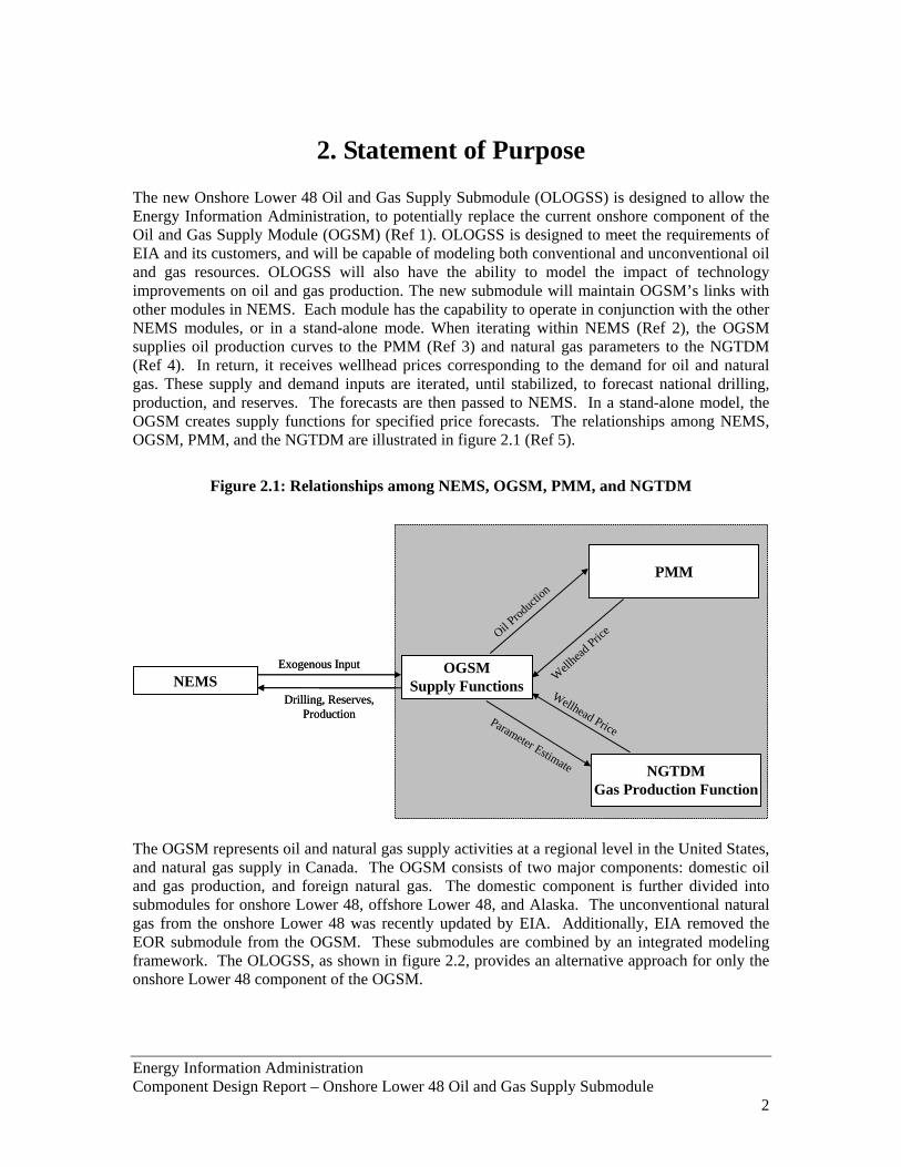
2. Statement of Purpose The new Onshore Lower 48 Oil and Gas Supply Submodule (OLOGSS) is designed to allow the Energy Information Administration, to potentially replace the current onshore component of the Oil and Gas Supply Module (OGSM) (Ref 1). OLOGSS is designed to meet the requirements of EIA and its customers, and will be capable of modeling both conventional and unconventional oil and gas resources. OLOGSS will also have the ability to model the impact of technology improvements on oil and gas production. The new submodule will maintain OGSM’s links with other modules in NEMS. Each module has the capability to operate in conjunction with the other NEMS modules, or in a stand-alone mode. When iterating within NEMS (Ref 2), the OGSM supplies oil production curves to the PMM (Ref 3) and natural gas parameters to the NGTDM (Ref 4). In return, it receives wellhead prices corresponding to the demand for oil and natural gas. These supply and demand inputs are iterated, until stabilized, to forecast national drilling, production, and reserves. The forecasts are then passed to NEMS. In a stand-alone model, the OGSM creates supply functions for specified price forecasts. The relationships among NEMS, OGSM, PMM, and the NGTDM are illustrated in figure 2.1 (Ref 5).

Figure 2.1: Relationships among NEMS, OGSM, PMM, and NGTDM

NEMSExogenous Input

Drilling, Reserves, Production

OGSMSupply Functions

PMM

NGTDMGas Production Function

Oil Prod

uction

Wellhea

d Pric

e

Wellhead PriceParameter Estimate

NEMSExogenous Input

Drilling, Reserves, Production

OGSMSupply Functions

PMM

NGTDMGas Production Function

Oil Prod

uction

Wellhea

d Pric

e

Wellhead PriceParameter Estimate

The OGSM represents oil and natural gas supply activities at a regional level in the United States, and natural gas supply in Canada. The OGSM consists of two major components: domestic oil and gas production, and foreign natural gas. The domestic component is further divided into submodules for onshore Lower 48, offshore Lower 48, and Alaska. The unconventional natural gas from the onshore Lower 48 was recently updated by EIA. Additionally, EIA removed the EOR submodule from the OGSM. These submodules are combined by an integrated modeling framework. The OLOGSS, as shown in figure 2.2, provides an alternative approach for only the onshore Lower 48 component of the OGSM.


Figure 2.2: Subcomponents within OGSM

OGSM

Domestic Foreign

Onshore Offshore AlaskaThe new “OLOGSS”

OGSM

Domestic Foreign


OGSM

Domestic Foreign


OGSM

Domestic Foreign

Onshore Offshore Alaska

Oil

The new “OLOGSS”

Gas

Known Fields- Conventional- Unconventional

Undiscovered- Conventional- Unconventional



OGSM

Domestic Foreign


OGSM

Domestic Foreign


OGSM

Domestic Foreign


OGSM

Domestic Foreign

Onshore Offshore Alaska

Oil

The new “OLOGSS”

Gas









2.1. Resources Modeled

2.1.1. Oil Resources Oil resources, as illustrated in figure 2.3, are divided into known fields and undiscovered fields. The OLOGSS models both conventional and unconventional oil resource. For the conventional known resource, production techniques are used for quantifying the production profiles from known fields under primary, secondary, and tertiary recovery processes. Resources under primary are also quantified for their improved oil recovery (IOR) processes that include profile modification, water flooding, infill drilling, and others. Known resources/ fields are evaluated for their upside potential using enhanced oil recovery (EOR) processes, including CO2 flooding, steam flooding, polymer flooding and chemical flooding. The unconventional known resource includes highly fractured continuous zones such as Austin chalk formations and Baken Shale formations. Certain oil shale and tar sand formations are included for evaluation. Undiscovered conventional and unconventional resources are characterized in a method similar to that used for discovered resource and evaluated for their potential from primary and secondary production techniques. The potential from the undiscovered resource is defined based on United States Geological Survey (USGS) estimates. These estimates are developed from detailed geological characterization of producing plays.


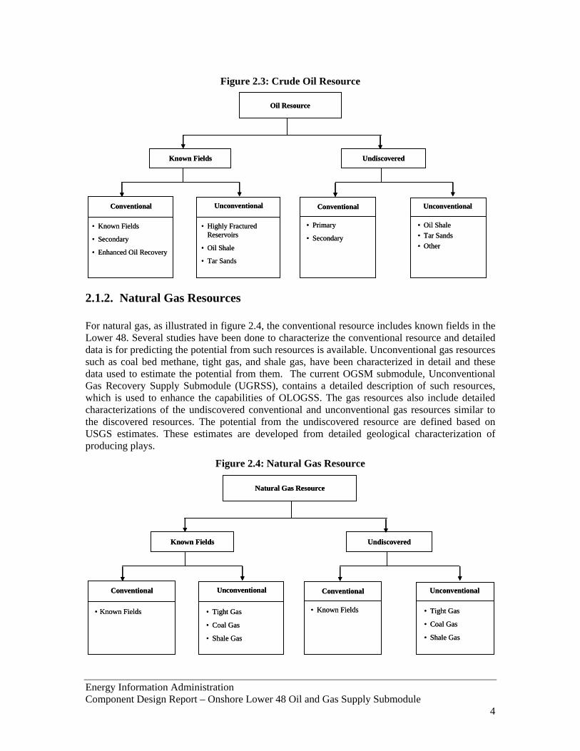
Figure 2.3: Crude Oil Resource

Oil Resource

Known Fields Undiscovered

Unconventional

• Oil Shale• Tar Sands• Other

Conventional

• Primary

• Secondary

Unconventional

• Highly Fractured Reservoirs

• Oil Shale

• Tar Sands

Conventional

• Known Fields

• Secondary

• Enhanced Oil Recovery

Oil Resource


Unconventional

• Oil Shale• Tar Sands• Other

Conventional

• Primary

• Secondary

Unconventional

• Highly Fractured Reservoirs

• Oil Shale

• Tar Sands

Conventional

• Known Fields

• Secondary

• Enhanced Oil Recovery

2.1.2. Natural Gas Resources For natural gas, as illustrated in figure 2.4, the conventional resource includes known fields in the Lower 48. Several studies have been done to characterize the conventional resource and detailed data is for predicting the potential from such resources is available. Unconventional gas resources such as coal bed methane, tight gas, and shale gas, have been characterized in detail and these data used to estimate the potential from them. The current OGSM submodule, Unconventional Gas Recovery Supply Submodule (UGRSS), contains a detailed description of such resources, which is used to enhance the capabilities of OLOGSS. The gas resources also include detailed characterizations of the undiscovered conventional and unconventional gas resources similar to the discovered resources. The potential from the undiscovered resource are defined based on USGS estimates. These estimates are developed from detailed geological characterization of producing plays.

Figure 2.4: Natural Gas Resource

Natural Gas Resource


UnconventionalConventional

• Known Fields

Unconventional

• Tight Gas

• Coal Gas

• Shale Gas

Conventional

• Known Fields • Tight Gas

• Coal Gas

• Shale Gas

Natural Gas Resource


UnconventionalConventional

• Known Fields

Unconventional

• Tight Gas

• Coal Gas

• Shale Gas

Conventional

• Known Fields • Tight Gas

• Coal Gas

• Shale Gas


2.2. Major Enhancements of Proposed OLOGSS The new OLOGSS is a play-level model, which forecasts the oil and gas supply from the onshore Lower 48. The modeling procedure includes a comprehensive assessment method for determining the relative economics of various prospects based on future financial considerations, the nature of the undiscovered and discovered resource, prevailing risk factors, and the available technologies. The model evaluates the economics of future exploration and development from the perspective of an operator making an investment decision. Technology advances, including improved drilling and completion practices, as well as advanced production and processing operations are explicitly modeled to determine the direct impacts on supply, reserves, and various economic parameters. All model outputs are consistent with the current requirements of the OGSM model. The model is able to evaluate the impact of research and development (R&D) on supply and reserves. Furthermore, the model design provides the flexibility to evaluate alternative or new tax, environmental, or other policy changes in a consistent and comprehensive manner. The OLOGSS possesses the capability to address these issues, which affect the profitability of development through a variety of levers, which model:

• Development of new technologies • Rate of market penetration of new technologies • Costs to implement new technologies • Impact of new technologies on capital and operating costs • Regulatory or legislative environmental mandates • Key taxation provisions such as severance taxes, state or federal income taxes,

depreciation schedules, tax credits, etc. In addition, the OLOGSS has the capability to address resource base issues. The OLOGSS is based on explicit estimates for technically recoverable oil and gas resources for each source of domestic production (i.e., geographic region/fuel type combinations). Strict resource accounting is used to ensure that unrealistic depletion of the resource base does not occur. The OLOGSS is capable of addressing access issues concerning oil and gas resources located on federal lands. Undeveloped resources will be divided into four categories:

• officially inaccessible • inaccessible due to development constraints • accessible with federal lease stipulations • accessible under standard lease terms


3. Background Research

3.1. Types of Oil and Gas Models Oil and gas supply models have historically relied on a variety of techniques to forecast future supplies. These techniques can be categorized generally as either geologic/engineering, econometric, or "hybrid". The geologic/engineering models are further disaggregated into play analysis models and discovery process models. The OLOGSS is a hybrid model, which applies the geologic and econometric techniques to specific resource types in order to predict the supply curves.

3.1.1. Geologic/Engineering Play analysis models are used for relatively undeveloped regions. This type of model relies upon detailed geological data and subjective probability assessments of the presence of oil or gas. Seismic data, expert assessments, and information from analog areas are utilized by a Monte Carlo simulator to generate a probability distribution of the total volume of oil or gas in a play. Discovery process models reflect the dynamics of the discovery process. They do not require detailed geological data. Instead, they rely upon historical exploratory drilling and discovery data. They are primarily used in areas already producing oil or gas. This type of model relies upon the assumption that larger oil or gas fields are more likely to be discovered. This assumption usually results in discovery rates which decline as the area becomes more explored. Both of these types of model typically include an economic component which determines the number of exploratory wells to be drilled. The number of wells that maximize the discounted net present value is the number of wells to be drilled. The economic component utilizes user specified oil and gas prices, costs, and taxes, as well as capital constraints.

3.1.2. Econometric Econometric models are based upon a system of equations. As applied to oil and gas, the typical econometric model has three equations representing: exploratory drilling, average oil and gas discovery sizes, and oil and gas success ratios. The product of these variables is the total new discoveries of oil and gas. Recently developed econometric models may include optimization principles that incorporate uncertainty, and general geologic trends and characterization. However, the geologic characterization is not as detailed as in the play analysis or discovery process models.

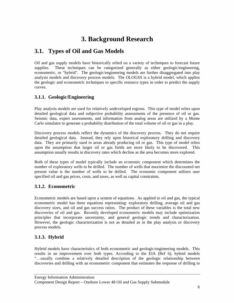
3.1.3. Hybrid Hybrid models have characteristics of both econometric and geologic/engineering models. This results in an improvement over both types. According to the EIA (Ref 6), hybrid models “…usually combine a relatively detailed description of the geologic relationship between discoveries and drilling with an econometric component that estimates the response of drilling to


economic variables. In this way, a time path of drilling may be obtained without sacrificing an accurate description of geologic trends.”

3.2. Oil and Gas Supply Models/Methodologies Considered Several publicly or commercially available models are widely used by the industry to predict oil and gas supply from the lower 48 onshore. Such models were evaluated against the following criteria:

1. The specific resource types evaluated by the model, including oil and gas, conventional and unconventional, and known fields and undiscovered resources.

2. Which unit of analysis, such as the region, basin, play, reservoir, or field, the model uses for its supply forecasts.

3. The types of reports provided by the model, such as price supply curves, drilling reports, economic reports, or reserve reports. Additionally, the levels of disaggregation at which these reports are made available (including national, regional, and state levels) were identified.

4. Other salient features of the models were identified. These features relate to the specific methodologies used to model oil and/or gas production, as well as the ability of the models to analyze technology or economic policy changes.

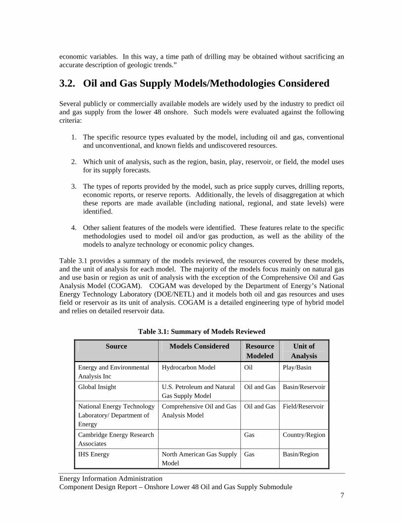
Table 3.1 provides a summary of the models reviewed, the resources covered by these models, and the unit of analysis for each model. The majority of the models focus mainly on natural gas and use basin or region as unit of analysis with the exception of the Comprehensive Oil and Gas Analysis Model (COGAM). COGAM was developed by the Department of Energy’s National Energy Technology Laboratory (DOE/NETL) and it models both oil and gas resources and uses field or reservoir as its unit of analysis. COGAM is a detailed engineering type of hybrid model and relies on detailed reservoir data.

Table 3.1: Summary of Models Reviewed

Source Models Considered Resource Modeled

Unit of Analysis

Energy and Environmental Analysis Inc

Hydrocarbon Model Oil Play/Basin

Global Insight U.S. Petroleum and Natural Gas Supply Model

Oil and Gas Basin/Reservoir

National Energy Technology Laboratory/ Department of Energy

Comprehensive Oil and Gas Analysis Model

Oil and Gas Field/Reservoir

Cambridge Energy Research Associates

Gas Country/Region

IHS Energy North American Gas Supply Model

Gas Basin/Region


The new OLOGSS is a hybrid model incorporating the best characteristics of the geologic/ engineering and econometric models. It can model the impact of technology improvements, legislative changes, and resource access changes, on the oil and gas supplies. These are modeled through the incorporation of technology, economic, tax policy, and resource access levers.


4. Input/ Output Requirements The new OLOGSS models both oil and gas resources and predicts future supply from the onshore Lower 48. The first step in defining the input/output requirements for the OLOGSS was defining the unit of analysis. This selection governed the input required for the model and the methodology for predicting supply from oil and gas resources. The following sections in this chapter define the unit of analysis required, its classification levels, and the input required by the new OLOGSS.

4.1. Unit of Analysis Defining the unit of analysis is a critical first step in any model design because it defines the model’s scope. Its selection is often limited because of the nature of the data available on regular basis. The unit of analysis also governs the model structure and issues related to maintainability and usability of the proposed model. The unit of analysis for OLOGSS was established after detailed evaluation of several data sources for their regular availability, cost and quality of data. The unit of analysis for OLOGSS and model structure should meet the following criteria:

1. Ability to model technology levers 2. Ability to model economic policy changes and levers 3. Ability to model resource access issues 4. Availability and ease of update 5. Fast execution time

Based on the above criteria, the following units of analysis were considered for OLOGSS: Reservoir: The occurrence of reservoir rocks of sufficient quantity and quality to permit the containment of oil and/or gas in volumes sufficient for an accumulation of the minimum size. Pool: The basic geologic unit consisting of a single oil or gas deposit as defined by trap, charge, and reservoir characteristics of the play. Field: An individual producing unit consisting of a single pool or multiple pools of hydrocarbons grouped on, or related to, a single structural or stratigraphic feature. Accumulation: An accumulation is defined by the USGS as a discrete field or pool of hydrocarbon localized in a structural or stratigraphic trap by the buoyancy of oil or gas in water. Cell: A cell is a quarter of a square mile of land surface in continuous formations. These are coded by USGS as predominantly oil producing, gas producing, both oil and gas producing or dry. The resource in each cell is characterized by its estimated ultimate recovery based on geologic characteristics of the continuous formation/accumulation. Play: A play is defined as a set of known or postulated oil and/or gas accumulations sharing similar geologic, geographic, and temporal properties, such as source rock, migration pathways, timing, trapping mechanism, and hydrocarbon type (Ref 7). The geographic limit of each play represents the limits of the geologic elements that define the play. USGS geologists responsible


for each province defined and mapped the limits of the reservoir rock, geologic structures, source rock, and seal lithologies. The only exceptions to this are plays that border the federal-state water boundary. In these cases, the federal-state water boundary forms part of the play boundary. Each of these units of analysis was carefully studied for data sources and also for availability of such data on a regular basis. Two different units of analysis were chosen to define the resource data required for modeling oil and gas supply. For discovered resources, the play was chosen as the preferable unit of analysis. For undiscovered resources, the accumulation/cell distribution at play level was chosen as the unit of analysis. All resources described in the document will be described at this unit of analysis.

4.1.1. Bin Classification In order to further disaggregate the discovered play-level data into meaningful resource groupings, several classification units were identified. This disaggregation of the play level resource into smaller groups is done for the following reasons:

1. To distinguish between stripper, marginal, and other well categories for tax purposes. 2. To apply adequate operating and maintenance costs based upon depth. 3. To model technologies that affect different depth formations.

To meet EIA’s modeling requirements, for each play level resource, the number of existing producing wells are identified and grouped into categories based on their production volumes and producing intervals. The production volume categories are determined by the daily average production rate measured in barrels of oil equivalent (BOE). The producing zone interval is categorized by depth. Figure 4.1 describes the ranges of different bin sizes based on production volumes. For each size bin, depth ranges that meet the requirements for measuring various technologies and consistent with the cost data provided by the EIA’s “Cost and Indices for Domestic Oil and Gas Field Equipment and Production Operations” (Ref 8) and American Petroleum Institute’s (API) “Joint Association Survey of Drilling costs” (Ref 9) were identified.

Figure 4.1: Bin Classification for Size and Depth

Size Range Depth Depth Range Number of Wells 0-10 0-2000>10-15 >2000-4000>15-50 >4000-8000>50-100 >8000-12000>100 >12000-15000

>15000

for each size bin

Size (BOE/Day) Depth of Producing Zone (Feet)

4.2. Types of Data OLOGSS requires resource data, production data, cost data, and development constraint data as illustrated in figure 4.2. The resource and production data are used to calculate the annual production from existing reservoirs and fields, reserves growth and the potential production through exploration. The cost data, such as the capital and operating costs, are necessary for


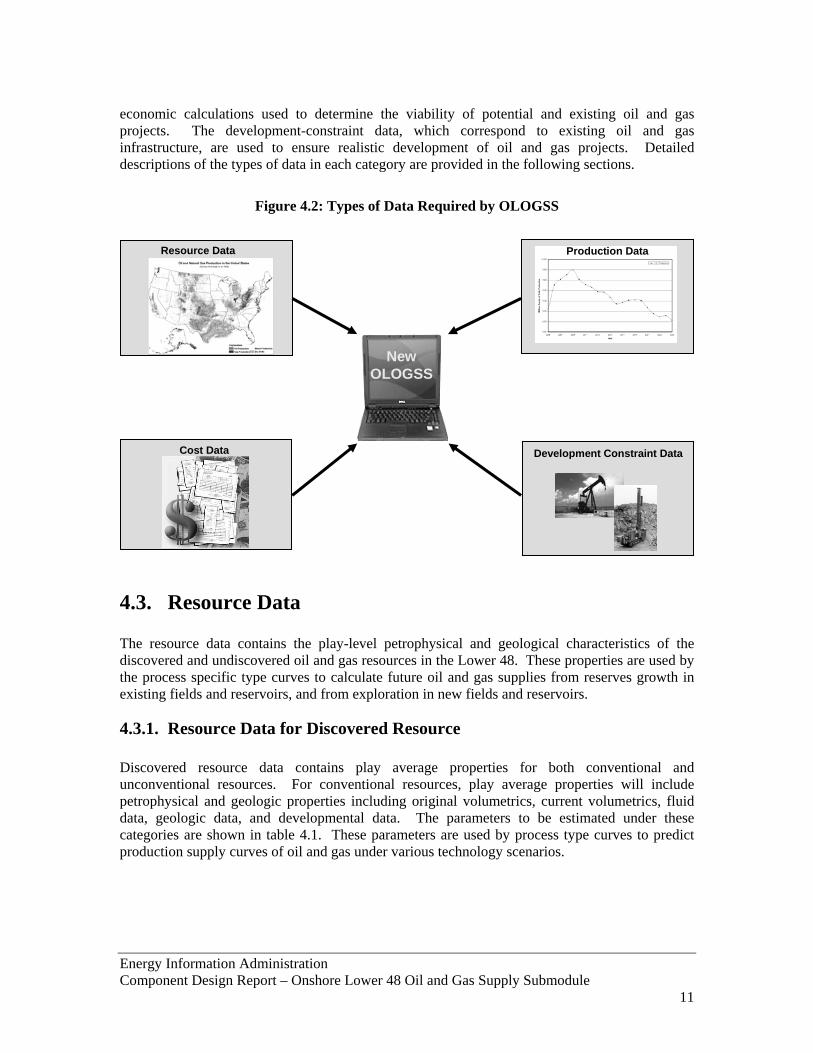
economic calculations used to determine the viability of potential and existing oil and gas projects. The development-constraint data, which correspond to existing oil and gas infrastructure, are used to ensure realistic development of oil and gas projects. Detailed descriptions of the types of data in each category are provided in the following sections.

Figure 4.2: Types of Data Required by OLOGSS

4.3. Resource Data

he resource data contains the play-level petrophysical and geological characteristics of the

4.3.1. Resource Data for Discovered Resource

iscovered resource data contains play average properties for both conventional and

Production Data Resource Data

New OLOGSS

Cost Data Development Constraint Data

Tdiscovered and undiscovered oil and gas resources in the Lower 48. These properties are used by the process specific type curves to calculate future oil and gas supplies from reserves growth in existing fields and reservoirs, and from exploration in new fields and reservoirs.

Dunconventional resources. For conventional resources, play average properties will include petrophysical and geologic properties including original volumetrics, current volumetrics, fluid data, geologic data, and developmental data. The parameters to be estimated under these categories are shown in table 4.1. These parameters are used by process type curves to predict production supply curves of oil and gas under various technology scenarios.


Table 4.1: Resource Data Categories

Original Volumetrics Geologic Data • Original-Oil-In-Place • Lithology • Reservoir Area • Depth • Net Thickness • Temperature • Porosity • Original and Current Pressure • Average Initial Water Saturation • Permeability • Average Initial Oil Saturation • Gross Thickness • Average Initial Gas Saturation • Dip Angle • Average Formation Volume Factor • Geologic Age Code

Current Volumetrics • Geologic Play, Depositional System, Trap Type

• Current Oil Saturation (Swept Zone) Fluid Data • Current Oil Formation Volume Factor • Average Oil Gravity and Viscosity

Development and Performance Data • Initial GOR

• Recovery Efficiency • Current GOR • Well Spacing • Gas Impurities

In addition to the parameters listed above, discovered resource estimates for various processes are used to ensure that the production forecasts do not exceed resource limitations. For unconventional oil resources, specialized databases available for Austin Chalk and Baken Shale formations are used. These databases provide average data at a county/basin level for continuous formations, and were developed in conjunction with industry experts. For unconventional gas, OGSM’s UGRSS contains a detailed play-level description of coalbed methane, tight gas sand, and gas shales. The data for UGRSS was derived using the 1995 USGS National Assessment of United States Oil and Gas Resources (Ref 10) and internal databases provided by an EIA contractor. These databases will be updated to reflect the 2005 USGS National Assessments. In addition to the average play-level properties, the discovered resource data includes basin, state, and regional averages for these same properties. These values are used to backfill any missing data for newly discovered plays.

4.3.2. Resource Data for Undiscovered Resource Conventional undiscovered resources are characterized at the accumulation level using the 2005 USGS updates to the 1995 National Assessment. For regions not included in the 2005 update, the 1995 assessment will be used. The USGS provides the accumulation size class distribution for the 700 plays grouped into 72 provinces. USGS fits a Truncated Shifted Pareto (TSP) distribution to assign data for discovered accumulations in a play and applies the data derived from the fitted distribution to estimate the number of undiscovered accumulations in the play. The product of estimated size distribution by the estimated frequency for undiscovered accumulations produces a resource estimate for a given play. USGS provides a detailed methodology and parameters to


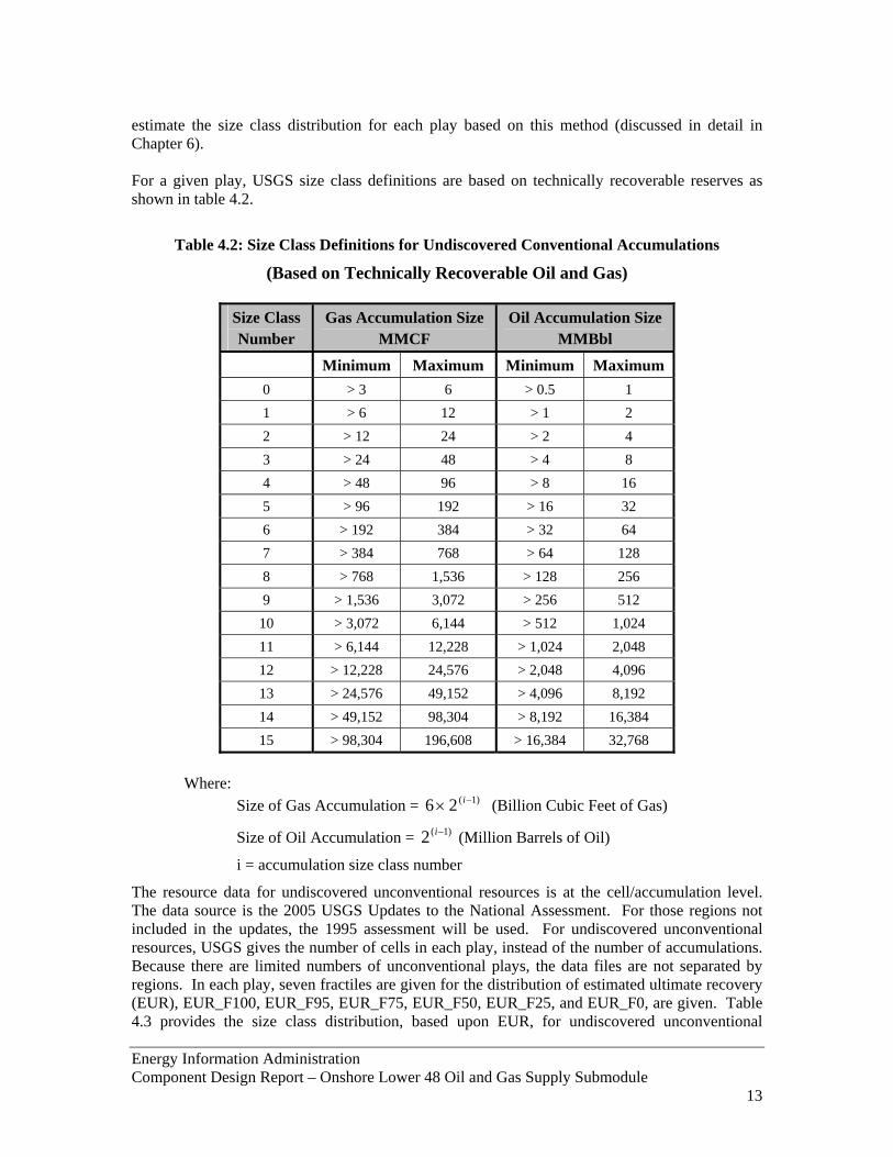
estimate the size class distribution for each play based on this method (discussed in detail in Chapter 6). For a given play, USGS size class definitions are based on technically recoverable reserves as shown in table 4.2.

Table 4.2: Size Class Definitions for Undiscovered Conventional Accumulations

(Based on Technically Recoverable Oil and Gas)

Size Class Number

Gas Accumulation Size MMCF

Oil Accumulation Size MMBbl

Minimum Maximum Minimum Maximum 0 > 3 6 > 0.5 1 1 > 6 12 > 1 2 2 > 12 24 > 2 4 3 > 24 48 > 4 8 4 > 48 96 > 8 16 5 > 96 192 > 16 32 6 > 192 384 > 32 64 7 > 384 768 > 64 128 8 > 768 1,536 > 128 256 9 > 1,536 3,072 > 256 512

10 > 3,072 6,144 > 512 1,024 11 > 6,144 12,228 > 1,024 2,048 12 > 12,228 24,576 > 2,048 4,096 13 > 24,576 49,152 > 4,096 8,192 14 > 49,152 98,304 > 8,192 16,384 15 > 98,304 196,608 > 16,384 32,768

Where:

Size of Gas Accumulation = (Billion Cubic Feet of Gas) )1(26 −× i

Size of Oil Accumulation = (Million Barrels of Oil) )1(2 −i

i = accumulation size class number

The resource data for undiscovered unconventional resources is at the cell/accumulation level. The data source is the 2005 USGS Updates to the National Assessment. For those regions not included in the updates, the 1995 assessment will be used. For undiscovered unconventional resources, USGS gives the number of cells in each play, instead of the number of accumulations. Because there are limited numbers of unconventional plays, the data files are not separated by regions. In each play, seven fractiles are given for the distribution of estimated ultimate recovery (EUR), EUR_F100, EUR_F95, EUR_F75, EUR_F50, EUR_F25, and EUR_F0, are given. Table 4.3 provides the size class distribution, based upon EUR, for undiscovered unconventional


resources. These size classes though not provided by USGS were used by NETL’s COGAM model and derived after discussions with USGS experts (Ref 11).

Table 4.3: Size Class Definitions for Undiscovered Unconventional Accumulations

(Based on Estimated Ultimate Recovery (EUR)) Size Class Number

Gas EUR Volume MMCF

Oil EUR Volume MBbl

Minimum Maximum Minimum Maximum 1 > 0 36 > 0 6 2 > 36 72 > 6 12 3 > 72 120 > 12 20 4 > 120 180 > 20 30 5 > 180 300 > 30 50 6 > 300 450 > 50 75 7 > 450 600 > 75 100 8 > 600 1,200 > 100 200 9 > 1,200 1,800 > 200 300

10 > 1,800 3,000 > 300 500

4.4. Production Data The production data includes the monthly, annual, and cumulative oil and gas production from discovered resources. The EIA Dallas Field Office (DFO) collects well level production data from HPDI and aggregates it to the field level. For the purpose of this model, the DFO will provide field level production data which will be further aggregated to the play level. This data is used, by the timing and economic module, to forecast production from existing reservoirs and fields using decline curve analysis. Production data for each play will be expressed as:

)odwell(Pr)od(Prn

ifieldresource,iresource,lplay ∑

=

=1

Where: i = the well number resource = 1 for oil and 2 for gas

prodwelli = the average production for well i, ifield = the number of fields lplay = the play number l, l = 1,…, maxplay Prod = the play level production for oil or gas

The aggregated play level production data will be validated against EIA production data contained in the Annual Energy Review.


4.5. Cost Data The Onshore Lower 48 Oil and Gas Supply Submodule requires cost data for economic calculations performed by the timing module. There are three broad categories of cost data required by the model: Capital costs, Operating costs, and other costs (Figure 4.3). The capital, operating, and other cost parameters are used in the timing/ economic module to calculate the lifecycle economics for all oil and gas projects. Process specific costs are used to calculate the economics for three types of projects (1) existing, (2) reserves growth, and (3) exploration. The development decisions for potential oil and gas reserves growth and exploration projects are based upon the economic viability of the project, and regional competition for resource development constraints.

Figure 4.3: Cost Data Requirements

Cost Data

Capital Costs Operating Costs

Variable O&M

• Lifting Cost• Gas Processing

Cost• Injection Costs• Injectant Costs• Other

Fixed O&M

• Fixed Annual Operating Costs

• Oil Well• Gas Well

• Secondary Production Cost

Resource/Process Specific

•Gas Processing Facilities

•Convert Primary to Secondary

•Convert Primary to Injector

•Water Treatment Plant•Other

•Drilling & Completion

•Workover

•Equipping Producers

•Other

Other Cost Parameters

•Royalty Rate

•Tax Rate•Federal•State

•Depreciation Schedule

•Depletion Rate

•Cost Multipliers

Cost Data

Capital Costs Operating Costs

Variable O&M

• Lifting Cost• Gas Processing

Cost• Injection Costs• Injectant Costs• Other

Fixed O&M

• Fixed Annual Operating Costs

• Oil Well• Gas Well

• Secondary Production Cost

Resource/Process Specific

•Gas Processing Facilities

•Convert Primary to Secondary

•Convert Primary to Injector

•Water Treatment Plant•Other

•Drilling & Completion

•Workover

•Equipping Producers

•Other

Other Cost Parameters

•Royalty Rate

•Tax Rate•Federal•State

•Depreciation Schedule

•Depletion Rate

•Cost Multipliers

Different capital and operating costs are required to do full life cycle economics of projects under a specific production process and a technology scenario. Tables 4.4 and 4.5 provide the types of capital and operating costs required for both oil and gas production processes which are considered for OLOGSS.

Table 4.4: Capital and Operating Costs for Oil Processes

Oil Process Modeled Capital Costs Operating Costs Decline Curve Analysis - None - Variable

- Operating

Horizontal Wells - Drilling and Completion - Workover

- Variable - Annual

Advanced Secondary Recovery (ASR)


- Infill Drilling - Drilling and Completion - Conversion of Producer to Injector - Workover - Water Treatment Plant

- Variable - Annual - Water Treatment

- Profile Modification - Drilling and Completion - Conversion of Producer to Injector - Workover - Water Treatment Plant - Polymer Handling Plant

- Variable - Annual - Water Treatment - Polymer

Enhanced Oil Recovery (EOR)

- CO2 Flooding - Drilling and Completion - Conversion of Producer to Injector - CO2 Recycling and Injection Plant

- Variable - Annual - CO2 Costs

- Steam Flooding - Drilling and Completion - Conversion of Producer to Injector - Steam Generator

- Variable - Annual - Steam Injection Cost

Table 4.5: Capital and Operating Costs for Gas Processes

Gas Process Modeled Capital Costs Operating Costs Decline Curve Analysis - None - Variable

- Annual - Gas Processing Costs

Reserves Growth - Drilling and Completion - Gas Treatment Costs

- Variable - Annual - Gas Processing Costs

In the following sections, the specific costs, the data sources, and the forms of the equations are detailed for the capital, operating, and other cost parameters.

4.5.1. Capital Costs Capital costs encompass the costs of drilling and equipment necessary for the production of oil and gas resources. There are two types of capital costs: (1) resource /process independent costs, and (2) resource/process specific capital costs. The resource independent capital costs pertain to all recovery methods and do not vary with the specific technology implemented in the project. Examples of these costs are: drilling and completion and well equipment costs. The resource/ process specific capital costs pertain to the specific recovery technology applied to the project. Examples include steam injection plants, CO2 injection plants, and gas processing facilities. Resource/Process Independent Capital Costs:


As shown in tables 4.4 and 4.5, resource independent capital costs are applied to both oil and gas projects, regardless of the recovery method applied. The major resource independent capital costs are: (1) drilling and completion costs, (2) workover costs, and (3) the costs to equip a primary producer. The costs to equip a primary producer include both surface and subsurface facilities. Drilling and Completion Costs: Drilling and completion costs incorporate the costs to drill and complete an oil or gas well (including tubing costs), and logging costs. These costs do not include the cost to drill a dry hole/wildcat during exploration. OLOGSS will have separate costs for dry holes drilled. For this analysis, the actual D&C costs will be obtained from the American Petroleum Institute's (API) publication, "Joint Association Survey On Drilling Costs" (JAS) (Ref 13). The JAS report provides data such as: number of wells, total footage drilled, and total drilling costs, for 10 different well-depth intervals within each state/region. JAS data will be used to calculate drilling costs as a function of depth and other parameters. Vertical well drilling costs include drilling and completion of the vertical, tubing and logging costs. Separate drilling cost equations are required for horizontal wells. For vertical wells, the drilling and completion cost is a function of the depth of the well and varies y by region. Vertical well drilling cost is defined as:

ii )depth(f)Well/$K(tcos_vert_Drill = Where:

depth = depth of producing formation (FT) i = OLOGSS region Where as, the horizontal well cost includes cost for drilling and completing a vertical well and the horizontal lateral(s). Horizontal well cost can be defined as:

ii )latlength,numlat,depth(f)Well/$K(tcos_horz_Drill = Where: Depth = depth of producing formation (FT) numlat = number of laterals latlength = length of each lateral (FT) i = OLOGSS region

Workover costs: Workover, also known as stimulation is done every 2-3 years to increase the productivity of a producing well. In some case workover or stimulation of wellbore is required to maintain production rates. Workover/Stimulation costs will be derived based on historical data published in Society of Petroleum Engineers (SPE) (Ref 14) and Gas Technology Institute (GTI) (Ref 15) literature. Workover cost is a function of depth of the producing interval and efficiency of stimulation.


ii effStimdepthfWellKWorkover )_,()/$( = Where: depth = depth of producing formation (FT) stim_eff = Efficiency of Stimulation i = OLOGSS region Costs to Equip a Primary Producer: The cost of equipping a new producing well includes the production equipment costs for primary recovery. The data used to calculate the cost to equip a primary producer is obtained from the Energy Information Administration (EIA) (Ref 16). These costs are a function of depth and allocated at a regional level.

ii )depth(f)Well/$K(imaryPr_Equip = Where:

depth = depth of producing formation (FT) i = OLOGSS region Exploratory Drilling Costs: The exploratory drilling costs are regional averages calculated as a function of the regional development drilling costs. The cost is a function of depth and allocated by region.

ii multtvertDrillfWellKtdrillEXP )exp_,cos__()/$(cos__ = Where:

Drill_vert_cost = Cost for drilling a vertical well Exp_mult = Region specific exploration cost multiplier (0 – 1) i = OLOGSS region Other resource/process independent capital costs to be identified will be incorporated into OLOGSS. Resource/Process Specific Capital Costs: The resource/ process specific capital costs are specific to the recovery method. These costs include the costs to convert primary wells to either secondary or injection wells, and the costs of the plants required for injection for various oil processes. Examples of plants include water treatment and water injection plants. Additional capital costs may be identified and incorporated into OLOGSS. Gas Processing and Treatment Facilities: One cost specific to natural gas production is the processing and treatment of gas. This cost is calculated based on the concentration of impurities present, such as water, carbon dioxide, nitrogen, hydrogen sulfide, and natural gas liquids in the gas stream. The capital costs for gas processing are a function of the impurities in the gas:

),,,()/($cos__22 NGLNSHCO ConcConcConcConcfmcftproccap =

Where: ConcCO2

= Concentration of Carbon Dioxide


ConcH2S = Concentration of Hydrogen Sulfide

ConcN = Concentration of Nitrogen ConcNGL = Concentration of Natural Gas Liquids Costs of Converting a Primary to a Secondary Well: These costs consist of the additional cost to equip a new producing well for secondary recovery. The cost of replacing the old producing well equipment includes the costs for drilling and equipping water supply wells, but excludes tubing costs. The data used to calculate the cost of converting a primary to a secondary are obtained from the EIA (Ref 17).

ii )depth(f)Well/$K(Sec_Conv = Where:

depth = depth of producing formation (FT) i = OLOGSS region Costs of Converting a Producer to an Injector: Producing wells may be converted to injection service because of pattern selection and the favorable cost comparison against drilling a new well. The conversion procedure consists of removing surface and sub-surface equipment (including tubing), acidizing and cleaning out the wellbore, and installing new 2-7/8 inch plastic-coated tubing and a waterflood packer (plastic-coated internally and externally). These costs are determined for certain depths in feet for each of the pertinent regions, and linear fits will be made of the costs versus depth data. These costs will be used on an average basis for various ASR/EOR processes which will be modeled to determine reserves growth. The data used to calculate the cost of converting a producer to an injector is obtained from the EIA (Ref 18). These costs are a function of depth and allocated at a regional level.

ii )depth(f)Well/$K(inj_Conv =

Where: depth = depth of producing formation (FT) i = OLOGSS region Cost of a Produced Water Handling Plant: The capacity of the water treatment plant is a function of the maximum daily rate of water injected and produced (MBbl) throughout the life of the project. The cost of the plant is a function of this capacity defined as:

)rate(maxf)Well/$K(tcos_treatplant_Water =

Where: maxrate = maximum daily water produced and injected rate (Mbbl) Cost of a Water Injection Plant: The capacity of the water injection plant depends on the maximum daily rate of water injected throughout the life of the project. The cost of such plant is dependent on this maximum rate and is defined as:

)rate(maxf)Well/$K(tcos_injplant_Water =

Where: maxrate = maximum daily water injection rate (Mbbl)


Cost of a Polymer/chemical Handling Plant: The capacity of the polymer/chemical handling plant is a function of the maximum daily rate of polymer/chemical injected throughout the life of the project. This cost of such plat is dependent on this maximum injection rate of the injectant and is defined as:

)rate(maxf)Well/$K(tcos_Polyplant =

Where: maxrate = maximum daily injectant injection rate (Mlbs) Cost of a C02 Recycling / Injection Plant: The capacity of a recycling/injection plant is a function of the maximum daily injection rate of CO2 (Mcf) throughout the project life. If the maximum CO2 rate is equal to or greater than 60 MBbl/Day then the costs are divided into two separate plant costs. Capital costs based on this rate are as follows:

)rate(maxf)Well/$K(tcos_plantCO =2 Where: maxrate = maximum daily CO2 injection (Mbbl) In addition to the capital cost mentioned here, several other resource specific costs may be identified for processes not now considered in this document.

4.5.2. Operating Costs In addition to the capital costs, economic model uses operating cost functions to calculate the full life cycle economics of the prospect. Operating costs consist of normal daily expenses and surface maintenance. As illustrated in figure 4.3, operating costs are divided into two categories: (1) fixed operating costs and (2) variable operating costs. Each of these categories, and their constituent costs will be described in the following sections. Fixed O&M Costs: There are two types of operating costs: (1) fixed annual costs (2) and fixed annual costs for secondary operations. The fixed annual operating costs will be applied to both oil and gas projects in decline curve analysis. The fixed annual costs for secondary wells will be applied to the reserves growth projects for oil and gas. Fixed Annual Cost: Fixed O&M costs for oil and gas wells are calculated from the "Costs and Indices for Domestic Oil and Gas Field Equipment and Production Operations" (Ref 19) an EIA annual report. Fixed O&M costs have a fixed component on a per well basis and a cost component which is dependent of the depth of the formation. These costs are defined as:

ii depthomincfixedfWellKprimarytOp ),_,()/$(_cos = Where:

Fixed = a fixed O&M cost (K$/well) Inc_om = an incremental O&M cost (K$/well feet)

depth = depth of producing formation (FT) i = OLOGSS region


Annual Costs for Secondary Production: The direct annual operating expenses include costs in three major areas: normal daily expenses, surface maintenance, and subsurface maintenance. EIA’s publication of "Costs and Indices for Domestic Oil and Gas Field Equipment and Production Operations" (Ref 20) provides secondary operating costs for West Texas only. These costs are dependent on the depth of the producing interval and are defined as:

)_,()/$(sec_ factorregdepthfWellKondaryCost = Where:

depth = depth of producing formation (FT) reg_factor = factor for regional adjustment For other areas, the secondary recovery operating maintenance costs are determined by multiplying the costs in West Texas by the ratio of primary operating costs. This method was used in the National Petroleum Council’s (NPC) EOR Study of 1984 (Ref 21) and was further validated using actual costs from vendors. Table 4.6 provides the regional factors used by COGAM to calculate costs for other regions. These factors will be validated using the latest Costs and Indices for Domestic Oil and Gas Field Equipment and Production Operations (Ref 22).

Table 4.6: Regional Cost Ratios for Secondary Production Operating Costs

Region Depth Interval (FT) 0 – 2,000 >2,000 – 4,000 >4,000 – 8,000 >8,000

South Texas 1.77 1.67 1.52 1.42 South Louisiana 1.61 1.53 1.42 1.34 Oklahoma 0.90 0.93 0.97 1.00 Rocky Mountains 0.95 0.93 0.89 0.87 California 0.89 0.91 0.92 0.93

Variable O&M Costs: There are four major types of variable operating costs: (1) lifting costs, (2) gas processing costs, (3) injection costs, and (4) injectant costs. The lifting costs, injection costs, and Injectant costs are applied to EOR and ASR projects. Examples of injectant costs are the costs of polymer and CO2. The gas processing costs are applied to the reserves growth projects for gas. Lifting Costs: Incremental costs are added to primary and secondary flowing wells. These costs include pump operating costs, remedial services, workover rig services, and associated labor. These costs are a function of depth and allocated at a regional level.

ii )depth(f)Well/$K(lift_tcosOp = Where:

depth = depth of producing formation (FT) i = OLOGSS region


Gas processing costs: The operating costs are calculated for each of the processes modeled. OLOGSS will compute the gas upgrading costs (cost to bring the gas to pipeline quality) based on specified impurity levels. These costs ($/Mcf) are subtracted from the gas price before performing any economic decision making in the timing module. The variable operating costs for gas processing is a function of the impurities is the gas:

),,,()/($cos__22 NGLNSHCO ConcConcConcConcfmcftprocOp =

Where: ConcCO2

= Concentration of Carbon Dioxide ConcH

2S = Concentration of Hydrogen Sulfide

ConcN = Concentration of Nitrogen ConcNGL = Concentration of Natural Gas Liquids Injection Costs: Incremental costs are added to secondary injection wells. These costs include pump operating, remedial services, workover rig services, and labor associated with injection. These costs are a function of depth and allocated at a regional level.

ii )depth(f)Well/$K(inject_tcosOp = Where:

depth = depth of producing formation (FT) i = OLOGSS region Injectant Costs: The injectant costs are added to secondary injection wells. These costs are specific to the recovery method selected for the project. The types of costs and cost units for each recovery process are provided in table 4.7.

Table 4.7: Injectant Costs for EOR and ASR Processes

Process Type of Cost Cost Unit - Primary/Secondary Surfactant - $/Lb - Alkaline Agents - $/Lb Micellar/Surfactant Flooding

- Water Handling/ Injection - $/Bbl

- Polymer Injected - $/Lb Polymer Flooding

- Water Handling/ Injection - $/Bbl

- CO2 Purchasing - $/Mcf of CO2

- Recycling/ Compression - $/Mcf Carbon Dioxide (CO2)

- Water Injection - $/Bbl

- Water Disposal - $/Bbl of Water - Water Injection - $/Bbl of Steam Steam Flooding

- Operating Produced Water Plants - $/Bbl of Steam


The function for the variable operating costs of injectants has the form:

i)tcos,type(f)well/$K(ttaninjec_tcosop = Where: type = annual volume of process specific Injectant cost = unit cost for injectant i = OLOGSS region Other variable O&M costs may be identified and incorporated into OLOGSS.

4.5.3. Other Cost Parameters In addition to the capital and operating costs, OLOGSS economic module requires lease acquisition cost, geological and geophysical cost, overhead related cost factor, depreciation and amortization schedules, federal and state tax rates, production tax rates etc. to perform the detailed cashflow analysis of oil and gas prospects. These factors or multipliers are derived from historical data and conversations with industry representatives. Lease Bonus/Acquisition Factors: The lease bonus/acquisition cost factor is assumed to be a fraction of the total revenue that could be generated from the reservoir. The lease bonus/acquisition cost is calculated by multiplying the factor and the total collected revenue. Geological and Geophysical (G&G) Factors: These costs for performing any geological and geophysical activities are calculated as a fraction of the well costs. The G&G cost multiplier can be changed based on new technology and by technology penetration curves. The G&G costs for exploration are currently considered sunk and are used to estimate total capital expenditures only. General Costs and Administration Overhead Multipliers: In addition to the capital and operating expenses, certain portions of the cost for equipment is added for, but not limited to administration, accounting, contracting, and legal fees/expenses for the project. These expenses are calculated as a fraction of the total cost/expenditure on a yearly basis. The model uses amortization and depreciation schedules as per the IRS code (Ref 23). A depletion allowance rate is also incorporated. OLOGSS has levers allowing changes to these schedules and rates for various tax policy analyses. Federal income taxes are calculated based upon a marginal rate of 34.5 percent. State income taxes are calculated using state specific schedules and tax rates. Severance taxes, also known as production taxes, are estimated based on the actual state specific tax rate. OLOGSS has levers for changing these rates for various tax/ policy analysis. In summary, there are three broad categories of cost data used in the economic calculations performed by the OLOGSS. These are the capital costs, the operating costs, and the other cost parameters. The major sources of data for the capital and operating costs are the “Joint Annual Survey of Drilling Costs” by the American Petroleum Institute, and EIA’s “Oil and Gas Lease Equipment and Operating Costs”. These costs are supplemented, where necessary, through cost data obtained by a vendor survey. Tables 4.4 and 4.5 provide a crosswalk of the various costs outlined in this section with the processes modeled by OLOGSS. The vendor survey provides


process specific cost data for the different recovery technologies. Finally, the other cost parameters are obtained through various state, Federal and publicly available publications.

4.6. Development Constraint Data The principle function of the timing and economic module is to prioritize, rank and phase the development of individual oil and gas projects after all technology and economic criteria have been satisfied. The goal is to mimic the way oil and gas decisions are made by industry. The selection and development of these projects depend on certain constraints, some on the regional level, some on the national level and for certain projects it depends on recovery techniques being contemplated. The following section provides a detailed description of these constraints and the type of data that required by OLOGSS. Drilling constraints are bounding values used to determine the resource production in a given region. These constraints are limitations on exploration and development imposed by the existing drilling equipment. Sources for the data include EIA, private firms, and vendor surveys. Drilling constraints are dependent on the following: • Rig Capacity and Depth Rating: The rig capacity is calculated from the number of

historical rigs for various drilling depths for both oil and gas. The number of rigs, their depth rating and their types will be used to determine the starting conditions for every region. Rig capacity in the model grows or shrinks depending upon the need for drilling based on gas prices. Rig retirement rates and rig construction rates are also provided based on interpretations of historical data and conversation with rig vendors such as Baker Hughes.

• Rig Utilization Rate: The rig utilization rate is calculated within the new OLOGSS based on

the amount of drilling needed in a year. The rig utilization rate drives the drilling cost because costs for rigs fall as the demands for rigs falls As rig utilization increases the costs of using rigs also increases because of the increased demand for rigs, up to the full drilling cost.

• Rig Retirement Rate: This represents the national annual average percentage of the lost

drilling capability due to rig retirement yearly. Oil and Gas Journal, EIA and JAS data will be used to estimate this percentage.

• Rig Mobilization (%): The ability for the drilling rigs to mobilize from one region to

another. Possible sources for data included IHS Energy, Smith Bits, and Baker Hughes. Drilling capacities constrain the amount of footage available for drilling in a given year. There are two types of footage constraints incorporated into OLOGSS: (1) developmental and (2) exploratory. They correspond to the total footage available to reserves growth and exploration projects. An additional drilling capacity constraint is the drilling growth rate. Each of these three drilling capacity constraints will be described in further detail.

Development (feet/year): The regional capacity for developmental drilling is based on analysis of the last 10 years of historical data. This analysis determines the maximum percentage by which the capacity in a region can increase within a year. JAS data and Independent Petroleum Association of America (IPAA) state reports (Ref 24) are used to


derive the drilling capacity. Development drilling capacity is specified for both vertical wells and horizontal wells. Both type of development drilling capacities are used in the model in determining drilling decisions. In addition, the actual number, and types of available rigs is used as an input. Exploration (feet/year): Exploration drilling capacity is derived using the same methodology as for development drilling. Drilling Growth (%): The percentage growth in drilling in each region is based on an analysis for the last 10 years of drilling footage data by region.

In summary, drilling constraints can be expressed as a function of oil price. An analysis of the historical data shows a lag between changes in oil prices and changes in available drilling footage. This relationship is shown in figure 4.4, which graphs oil prices and available footage over time.

Figure 4.4: Relationship Between Oil Price and Available Drilling Footage

0

5

10

15

20

25

30

1987 1989 1991 1993 1995 1997 1999

Year

Oil

Pric

e (2

000

$/B

bl)

0

20

40

60

80

100

120

140

160

180

Tot

al D

rilli

ng (M

M F

T)

Oil PriceTotal Drilling

Source: EIA Historical Data

The lag coefficient shown in figure 4.4 will be incorporated into the drilling footage function. The form of the function is as shown below:

iyriyriyriyriyr growthoilpricefootagedrillingfFTfootageDrilling ),,_()(_ 111 −−−= Where: iyr = current analyzed


iyr-1 = previous year drilling_footageiyr = total footage available in year iyr (FT) oilpriceiyr = oil price in iyr ($/Bbl) growthiyr = drilling growth rate in iyr Drilling growth in any given year is further defined as:

iyriyr mobilrigrateretrigrateconstrigfgrowth )_,__,__((%) = Where: Rig_const_rate = rate of rig construction Rig_ret_rate = rate of rig retirement Rig_mobil = percentage of rigs able to mobilize from other regions iyr = year of model analysis

4.6.1. Capital Constraints Oil and gas companies use different investment and project evaluations criteria based upon their specific cost of capital, the portfolio of investment opportunities available, and their perceived technical risks. OLOGSS uses capital constraints to mimic the limitations on the amount of investments the oil and gas industry can make in a given year. The source of this data is the EIA (Ref 25).

4.6.2. Other Development Constraints Two other types of development constraints will be considered: (1) Carbon Dioxide availability and (2) resource access. These constraints are applied to the selection of projects within the economic/ timing module. They will be described in the following sections. Carbon Dioxide (CO2) Availability: For CO2 Miscible flooding, availability of CO2 gas from natural and industrial sources is a limiting factor in developing the candidate projects. In the Permian Basin, where the majority of the current CO2 projects are located, the CO2 pipeline capacity is a major concern. Efforts will be expended to compile information on the current and future capacity of these pipelines and also on the future volume and availability of the CO2 in other regions for use in the integrated system. Detailed data for CO2 sources and pipelines are available from Kinder Morgan and the annual Oil and Gas Journal EOR issue. Resource Access: The access to Federal lands is a constraint on both oil and gas development, particularly for undiscovered resources. Efforts will be expended to compile relevant information available through the BLM and the MMS for use in the integrated system. Provisions of the Energy Policy and Conservation Act (EPCA), reauthorized in 2003, require federal agencies to develop a national inventory of all oil and gas resources and reserves beneath federal land. These resources are divided into three access categories:

• •

•

No Leasing (Off Limits) Leasing with Restrictions on Drilling

No Surface Occupancy


Controlled Surface Occupancy • •

• Drilling Limitations (from <3 months to >9 months)

Leasing with Standard Lease Terms (SLT)

Federal lands access levers in the modeling system will be based on these three access categories. The OLOGSS is capable of handling new data as further studies are made available. This framework will help policy makers understand the impact of various leasing terms and options. In summary, the development constraints limit the annual development of oil and gas projects. These constraints are based upon the infrastructure of the oil and gas industry, and resource access limitations. They are applied within the timing/ economic module to the reserves growth and exploration projects. The sources of development constraint data include the EIA, BLM, USGS, and vendors. From EIA, data about capital expenditures will be gathered. From BLM and USGS, data pertaining to the access to the resource on federal lands will be obtained. API, IPAA, and Oil and Gas Journal data will be used to determine drilling constraints. Finally, the other development constraints data, such as the availability of CO2, and the number and types of rigs available, will be gathered from vendors.


5. Classification Plan

5.1. Definition of Regions In the Onshore Lower 48 Oil and Gas Supply Submodule, the oil and gas resources are represented by seven geographic regions. The regions were chosen in light of historical, developmental, and reporting considerations. The regions were selected based upon the following rationale: • Maintaining continuity with the historical output series from the Annual Energy Outlook. • Ensuring that the technology development constraints are reflected in the analysis and

competition of various resources. For these reasons, the OLOGSS regions were derived from the OGSM onshore regions with the exception that the OGSM region 5 (Rocky Mountain) is divided into OLOGSS region 5 (Rocky Mountain) and OLOGSS region 7 (Northern Great Plains). This division reflects the differences in costs and development constraints between these two regions. The OLOGSS regions are illustrated in Figure 5.1 and listed in Table 5.1.

Figure 5.1: Onshore Lower 48 Oil and Gas Supply Submodule Regions


Table 5.1: Onshore Lower 48 Oil and Gas Supply Submodule Regions

Number Name State/ Sub-state Number Name State/ Sub-state Connecticut Arkansas Delaware Iowa District of Columbia Kansas Georgia Minnesota Illinois Missouri Indiana West Nebraska Kentucky East Nebraska Maine

3 Midcontinent

Oklahoma Maryland East New Mexico Massachusetts TX RRC District 7B Michigan TX RRC District 7C New Hampshire TX RRC District 8 New Jersey TX RRC District 8A New York TX RRC District 9 North Carolina

4 Southwest

TX RRC District 10 Ohio Arizona Pennsylvania East Colorado Rhode Island West Colorado South Carolina Idaho Tennessee Nevada Vermont Utah Virginia West New Mexico West Virginia

5 Rocky Mountain

Wyoming

1 East Coast

Wisconsin California Alabama Oregon Florida

6 West Coast

Washington North Louisiana Montana South Louisiana North Dakota Mississippi

7 Northern Great Plains

South Dakota TX RRC District 1 TX RRC District 2 TX RRC District 3 TX RRC District 4 TX RRC District 5

2 Gulf Coast

TX RRC District 6


6. Methodology Description

6.1. Model Objective The Onshore Lower 48 Oil and Gas Supply Submodule provides forecasts of crude oil and natural gas production. Crude oil production is differentiated by three specific API gravities. Natural gas production is categorized as non-associated or associated-dissolved, depending on whether it comes from predominantly gas or oil wells. Two major well types represent drilling in the OLOGSS. Exploratory wells are drilled in relatively untested or unproven areas and can result in the discovery of new fields or new pools within existing fields. Developmental wells are primarily within or near proven areas and can result in reserve extensions or revisions. Extensions and revisions come from infill drilling or, in the case of oil, from improved and enhanced oil recovery techniques. The OLOGSS also has the capability to model the improvements in production associated with technology improvements, economic and policy changes, and resource access changes.

6.2. Model Structure The OLOGSS is data-driven submodule and has a modular structure with five major components as shown in Figure 6.1.

• Master Database contains the raw resource and production data for the OLOGSS. This data contains discovered and undiscovered, as well as conventional and unconventional, oil and gas resources.

• Resource Description Module processes the raw data in the Master Database. It creates the resource data files used by the process module and the timing/ economic module.

• Process Module is an external module containing process-specific type curve functions. These functions are developed using commercially or publicly available simulators or process models.

• The Timing/Economic Module forecasts supply, conducts detailed cashflow analysis, and ranks potential oil and gas projects according to economic viability and likely success, and competes them for resource development constraints.

• The Reports Module passes the OLOGSS results to the other OGSM module, NEMS, and the user. These results include price and supply functions, as well as drilling statistics provided at several levels of aggregation.

The two types of external data files are the Exogenous Data Files and the Model Levers. The Exogenous Data Files contain the cost data and resource development constraints. These constraints are required for detailed cashflow analysis and the project development methodology. The Model Levers are user-specified values for technology, economic, tax, and resource access variables. They are used to control the OLOGSS run and to conduct technology, economic, and policy analyses. In the following sections, each of the system components is described in greater detail.


Figure 6.1: OLOGSS System Logic Flow

Master Database

Resource Description Module

Timing/Economic Module

Report Module

Exogenous Data Files:• Cost Files• Resource

Development Constraints

• Technology Levers• Economic Levers• Resource Access

Parameters

Process Module

Master Database



Report Module




Parameters

Process Module

Master Database



Report Module




Parameters

Process Module

6.2.1. Master Database Overview: The master database contains the raw data used by the process module and the economic/timing module. The master database is electronically linked to source files and includes procedures to preserve databases for unconventional gas already collected by EIA and other critical databases. Types of Data: The master database contains resource and production data, process-specific resource estimates, and undiscovered resource estimates. The resource data, as described in chapter 4, is at the play level and contain average petrophysical and geologic properties. Additional resource data, used for backfill purposes only, includes basin, state, and regional average properties. The production data includes historical annual and cumulative production at the well, state, and regional levels. The state- and regional-level data are used for quality-control procedures. Resource potential estimates are provided by process (production, reserves growth processes, and exploration) at the play level. The undiscovered resource estimates are at the accumulation level for conventional oil and gas, and the cell level for unconventional resources. Table 6.1 lists the source(s) for each of the four types of data.


Table 6.1: Sources of Resource Data

Required Data Source Well-Level Production Data HPDI Production Data Play-Level Properties Derived from COGAM data files

using NRG Data Undiscovered Resource Estimates USGS Files Regional/ Play Level Production EIA

6.2.2. Resource Description Module The resource description module processes the raw resource and production data contained within the master database and prepares the resource data files for the timing/economic module. As shown in Figure 6.2, the resource description module reads the databases stored in the master database (M1) and processes the data for the timing/ economic module. For discovered resources, the data is aggregated at play level (M2) and various size/depth bins are populated (M3). For undiscovered resources (M4), the resource estimates at play level are defined using USGS data (M5). Play-level average properties are assigned to each discovered bin and undiscovered size classes (M6), and the resource data files are created for the timing module (M7). Each step within the resource description module is further discussed in this section.

Figure 6.2: Resource Description Module Flowchart

Master Database

Discovered Resources Undiscovered Resources

Define Resource Estimates by Play

Aggregate Production at Play Level

Populate Various Bins

Assign Play Level Properties

Create Resource Files for Timing Module

M3

M2

M1 M4

M5

M6

M7

Master Database

Discovered Resources Undiscovered Resources

Define Resource Estimates by Play

Aggregate Production at Play Level

Populate Various Bins

Assign Play Level Properties

Create Resource Files for Timing Module

M3

M2

M1 M4

M5

M6

M7


Discovered Resources (M1): Data files within the Master Database are read. Those files containing resource data or production data for discovered oil and gas resources are tagged and passed on to step M2. Aggregate Production at the Play Level (M2): This step reads the discovered resource data passed from Step M1, and the USGS play-location files. It maps the production data for each well to the USGS plays and aggregates the production. These aggregations are validated against the EIA production data. The major steps performed include:

Step 1: Read the HPDI field production data and the EIA play level production data. Step 2: Map wells to the USGS defined play. Aggregate the production for both oil and

gas at the play level. Step 3: If the aggregated play-level production is different from the EIA production data,

prorate the aggregated production data to match.

The resulting data files are passed to step M3. Populate Bins (M3): This step populates the play-level bins for discovered resources. The resulting data files contain the number of wells by resource, size bin and depth bin, for each play and for each year analyzed by OLOGSS. The major steps performed include:

Step 1: Read the bin categorization file contained in the Master Database and define the size and depth bins.

Step 2: Use field production data to define a typical oil/gas well production profile and assign wells, as oil or gas, to a play based upon field characteristics.

Step 3: Use a decline-curve methodology, and the historical-production data, to forecast annual production throughout the well’s lifecycle

Step 4a: Determine the well’s production, in BOE, at the beginning of the first

year of analysis. Step 4b: Assign the well to the appropriate bin using the average production

calculated in step 4a and the depth of the producing zone. Step 4c: Repeat steps 4a and 4b for each year.

Figure 6.3 shows the production decline curves of three hypothetical wells in a play. The average production, relative to three size bin categories, is plotted over time. The production for each well is read at the points marked by the x’s. These values are used to assign the well to the corresponding size category bin. As seen in figure 6.3, the production of Well A locates it in size category 1 in the first and second years. As the production decreases, the well passes to size category 2 in year three and size category 3 in year six. Wells B and C change size categories in a similar manner. Note: As well level production data is not available; every well in a given field will have the same average production profile.


Figure 6.3: Hypothetical Decline Curves for Three Wells

x

Years1 2 3 4 5 6 7

SizeCategory 1

SizeCategory 2

SizeCategory 3

Well

Well

Well

Ave

rage

Dai

ly P

rodu

ctio

n(B

OEP

D

x x

x

x

xx

x

x

x

xx

xxx

xx

x

A

B

C

x

Years1 2 3 4 5 6 7

SizeCategory 1

SizeCategory 2

SizeCategory 3

Well

Well

Well

Ave

rage

Dai

ly P

rodu

ctio

n(B

OEP

D

x x

x

x

xx

x

x

x

xx

xxx

xx

x

A

B

C

Table 6.2: Corresponding Well Bin Population

Years

Bin 1 2 3 4 5 6 7

1 2 1 0 0 0 0 0

2 1 2 2 2 1 0 0

3 0 0 1 1 2 3 3

The well population in table 6.2 corresponds to the bin assignments of the three hypothetical wells. For Size Bin 1, there are two wells in the first year (Wells A and B), and one well in the second year (Well A). In the third and later years, there are zero wells in that bin. After the second year, the bin contains zero wells. The population of size bins 2 and 3 are determined in a similar manner.

Step 5: Repeat steps 2 to 4 for all wells. Step 6: Calculate the total number of wells in each play. Step 7: Validate the total number of wells in a play against EIA data

The outputs of this step are passed to step M6 Undiscovered Resources (M4): The resource data files for undiscovered resources contained within the Master Database are read. These files are tagged and passed on to step M5. Define Resource Estimates by Play (M5): This step determines the play-level resource estimates for undiscovered resources contained in data files identified by step M4. It applies a Truncated Shifted Pareto (TSP) Analysis to the USGS play-level data in order to determine the play-level


distribution of accumulations in each size class. The parameters for TSP are provided by USGS are unique for every play. The major steps performed include:

Step 1: Read the regional USGS files containing the total accumulations for each play, and the key parameters required for calculating the number of accumulations, using the Truncated Shifted Pareto Distribution.

Step 2a: Define the oil and gas size classes using USGS data files contained

within the Master Database. The size-class definitions for conventional and unconventional accumulations are listed in table 4.2 and table 4.3 respectively.

Step 2b: Calculate Tu

TuA

ksizekjsize

jGB

−

−+−

=

−

1

}]1

)),1(),(({[)(

1

Where: j = 1… 16 k = 1 for oil and 2 for gas A, B, and Tu are play parameters provided by the USGS

Step 2c: Determine the Accumulation Size class distribution by calculating ),()]1()([)( kiplayaccumentjGjGjUND ×+−= Where:

iplay = play being evaluated j = 1… 15 k = 1 for oil and 2 for gas

),( kiplayaccument = the number of oil or gas accumulations for play iplay .

Step 3: Repeat steps 1 and 2 for each play in each region.

The outputs of this step are passed to step M6 Assign Play-Level Properties (M6): Play-level properties are assigned to the bins (for discovered resources) and the accumulation size classes (for undiscovered resources). If play level characteristics are unavailable, basin or regional properties are used. The major steps for discovered resources include:

Step 1: Read the data files containing play level properties. Step 2: For discovered resources, assign play level properties to the various bins. Step 3: For undiscovered resources, assign average reservoir level properties for the size

classes to the various accumulations. If the size classes are not available, assign play, basin, or regional data in that order.

The resulting data files are passed on to step M7. Create Resource Files for Timing Module (M7): In this step, the data files prepared in step M6 are used to create the resource data files for the timing/ economic module. The resource data files


contain five types of data required by the process module and timing module: (1) historical production data, (2) bin populations, (3) play-level properties, (4) resource estimates for discovered resources, and (5) size-class distributions for undiscovered resources. The historical production data is used by the decline curve method, within the timing module, to forecast annual oil and gas production from known fields and reservoirs. The bin populations are used to create pseudo projects and forecast production through reserves growth in known fields. The play-level properties are used by the process module to screen reserves growth processes and forecast the production potential from reserves-growth projects. The resource estimates for discovered resources are used to ensure reasonable resource development schedules during the timing and selection step in the timing module. The size-class distributions for undiscovered resources are used to forecast production from exploration.

6.2.3. Process Module The process module is external to the OLOGSS structure. The purpose of this module is to estimate the onshore lower 48 oil and gas supply from production in existing fields and reservoirs, and from reserves growth in existing reservoirs. The production in existing fields and reservoirs is forecast using a decline curve methodology. Future production from reserves growth in existing fields and reservoirs is forecast using process-specific type curve functions. All production type curves are functions of process-specific technology levers and play-level petrophysical properties. The technology levers will be discussed in section 6.2.v. The variables in the functions are classified as either common or process-specific. The common variables, used by both resources and all processes are required by the lack of detailed and specific reservoir data in OLOGSS. The function forecasts the average incremental production associated with the specific reserves growth process. An example of a process specific type curve is the dashed line graphed in figure 6.4.

Figure 6.4: Example of Process Specific Type Curve

Time

Ave

rage

Dai

ly P

rodu

ctio

n (B

OE

)

Reserves Growth

Time

Ave

rage

Dai

ly P

rodu

ctio

n (B

OE

)

Reserves Growth


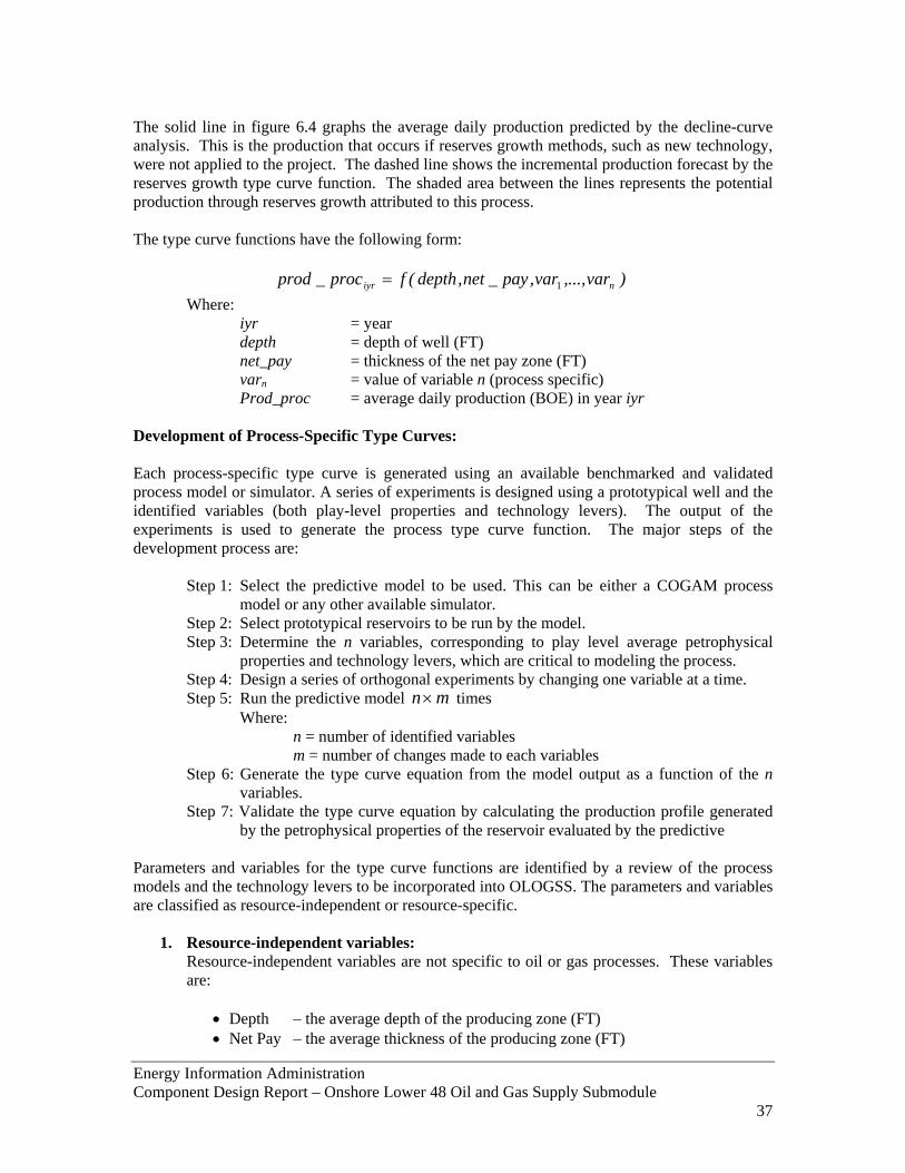
The solid line in figure 6.4 graphs the average daily production predicted by the decline-curve analysis. This is the production that occurs if reserves growth methods, such as new technology, were not applied to the project. The dashed line shows the incremental production forecast by the reserves growth type curve function. The shaded area between the lines represents the potential production through reserves growth attributed to this process. The type curve functions have the following form:

)var,...,var,pay_net,depth(fproc_prod niyr 1= Where: iyr = year depth = depth of well (FT) net_pay = thickness of the net pay zone (FT) varn = value of variable n (process specific) Prod_proc = average daily production (BOE) in year iyr Development of Process-Specific Type Curves: Each process-specific type curve is generated using an available benchmarked and validated process model or simulator. A series of experiments is designed using a prototypical well and the identified variables (both play-level properties and technology levers). The output of the experiments is used to generate the process type curve function. The major steps of the development process are:

Step 1: Select the predictive model to be used. This can be either a COGAM process model or any other available simulator.

Step 2: Select prototypical reservoirs to be run by the model. Step 3: Determine the n variables, corresponding to play level average petrophysical

properties and technology levers, which are critical to modeling the process. Step 4: Design a series of orthogonal experiments by changing one variable at a time. Step 5: Run the predictive model mn× times Where: n = number of identified variables m = number of changes made to each variables Step 6: Generate the type curve equation from the model output as a function of the n

variables. Step 7: Validate the type curve equation by calculating the production profile generated

by the petrophysical properties of the reservoir evaluated by the predictive Parameters and variables for the type curve functions are identified by a review of the process models and the technology levers to be incorporated into OLOGSS. The parameters and variables are classified as resource-independent or resource-specific.

1. Resource-independent variables: Resource-independent variables are not specific to oil or gas processes. These variables are:

• Depth – the average depth of the producing zone (FT) • Net Pay – the average thickness of the producing zone (FT)


• Varn – to be identified through a review of the process models

2. Resource-specific variables: Resource-specific variables are also process dependent for oil and gas resources. Examples of these variables are: • Oil-Specific Variables:

These variables are determined based upon the specific process used. Examples of oil-specific variables are identified in table 6.3.

Table 6.3: Process Specific Technology Levers for Oil

Process Dependent Variable ASR/ Waterflood PI, SORW, Volume Sweep EfficiencyEOR/ CO2 Flooding WAG Ratio EOR/ Steam Flooding Steam Override Horizontal Wells Length of Horizontal Lateral

Where:

PI = Productivity Index SORW = Saturation of Oil Remaining after Waterflood WAG ratio = Water Associated Gas ratio

• Gas-Specific Variables:

These variables are specific to the prediction of gas production from gas plays only. Examples of such variables are: • Pressure Gradient • Productivity Index • Recovery Efficiency

The remaining variables are identified through reviews of the existing R&D programs and the process models used to generate the equation data. These variables have corresponding model levers used for R&D analysis.

6.2.4. Economic/ Timing Module The economic/timing module forecasts the annual oil and gas production from existing fields, reserves growth, and exploration. It performs economic evaluation of the projects and ranks the reserves growth and exploration projects for development in a way designed to mimic the way decisions are made by the oil and gas industry. Development decisions and project selection depends upon economic viability and the competition for capital, drilling, and other available development constraints. Finally, the timing module aggregates production and drilling statistics using geographical and process specific categories. The timing/ economic module reads the resource data files created by the master database and the external data files in step A. Once the data is read, the timing module year loop begins. The play level bins are populated in step B using the resource data files. The discovered resources undergo


bin-level production decline curve and economic analysis in step D. The economic bins are marked for aggregation in step G, and the uneconomic bins are tagged for reserves growth in step E. In step E, potential reserves growth projects are created, the reserves growth potential is defined for each project and reserves growth economics are conducted. The resulting list of potential reserves growth projects is sent to project ranking in step F. The undiscovered resources are then explored, and the economics of potential exploration projects are evaluated in step C. The resulting ordered exploration project list is sent to project ranking in step F. In step F, the two lists of projects are combined and ranked on a regional level according to investment efficiency (for discovered projects) or probability of discovery (for undiscovered projects). The list is then passed to step G. The projects on the ranked list are timed, subject to regional development constraints, and their production is aggregated in step G. Steps B through G are then repeated for each year of analysis. After the final year, the results are sent to step H. In this step, the reports are generated and passed to other OGSM and NEMS modules, and the user. The structure of the timing/ economic module is illustrated in figure 6.5. Each step in the structure has been labeled and is described in detail in the following sections. Read Data (A): This submodule reads all of the external data files into the timing module. These files include the resource data files created by the resource description module. The other external files contain:

• Capital, operating, and other cost data (described in section 4.5) • Process type curve parameters (described in section 6.2.iii) • Development constraint data (described in section 4.6) • Oil and Gas prices • NEMS control variables • User defined data such as: (described in section 6.2.vi)

o Model run controls o Technology levers o Resource access parameters o Economic levers

Oil and gas prices come from one of two sources: an external price file or other NEMS modules. The source is determined by whether the model is run in a stand-alone mode or iterated within NEMS. If OLOGSS is run in a stand-alone mode, the model uses either fixed oil and gas prices or an annual price track. If OLOGSS is run within NEMS, the prices are generated by the iteration with the PMM and the NGTDM. Initial oil and gas prices are supplied to OLOGSS and used in the lifecycle economic calculations. The resulting supply functions are sent to the PMM and NGTDM. The prices corresponding to the demand calculated by these modules are passed back to OLOGSS and used to recalculate the supply functions. This process is repeated until prices, which stabilize supply and demand, are generated. The iterative process is repeated, using the previous year’s stabilized prices as an initial price, for each year evaluated by NEMS.


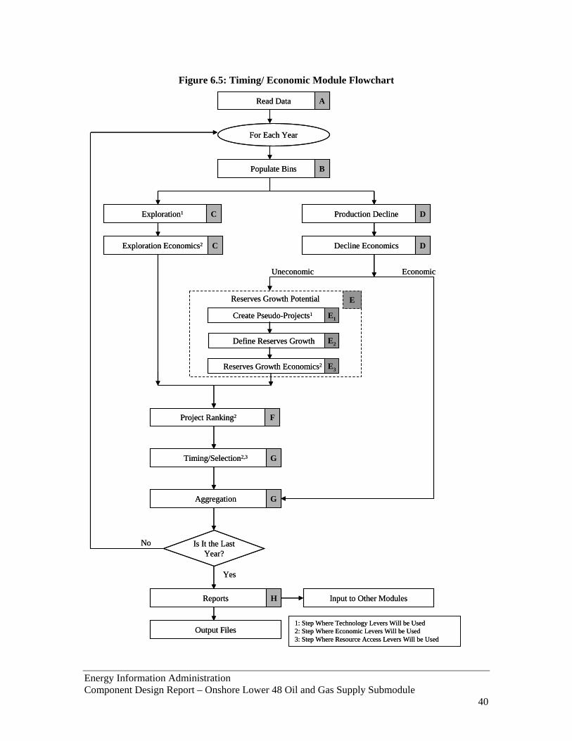
Figure 6.5: Timing/ Economic Module Flowchart

Economic

Read Data

For Each Year

Populate Bins

Exploration1

Exploration Economics2

Production Decline

Decline Economics

Create Pseudo-Projects1

Reserves Growth Economics2

C

A

B

D

D

Uneconomic

Project Ranking2

Timing/Selection2,3

Aggregation

G

G

Is It the Last Year?

Yes

No

Reports Input to Other Modules

Output Files

F

C

H

Reserves Growth Potential E

E1

E2Define Reserves Growth

E3

1: Step Where Technology Levers Will be Used2: Step Where Economic Levers Will be Used3: Step Where Resource Access Levers Will be Used

Economic

Read Data

For Each Year

Populate Bins

Exploration1

Exploration Economics2

Production Decline

Decline Economics

Create Pseudo-Projects1

Reserves Growth Economics2

C

A

B

D

D

Uneconomic

Project Ranking2

Timing/Selection2,3

Aggregation

G

G

Is It the Last Year?

Yes

No

Reports Input to Other Modules

Output Files

F

C

H

Reserves Growth Potential E

E1

E2Define Reserves Growth

E3

1: Step Where Technology Levers Will be Used2: Step Where Economic Levers Will be Used3: Step Where Resource Access Levers Will be Used


Populate Bins (B): In this step, the play-level bins for discovered resources are populated using the resource data files and the aggregated number of previously discovered wells from timed reserves growth projects. The major steps are:

Step 1: Assign the bin population generated by the resource description module. Step 2: Subtract the aggregated number of developed wells timed in step G.

An example of this methodology is provided in figure 6.6. Table A in figure 6.6,

corresponding to step 1, shows the hypothetical bin populated, for a play, by the resource description module. The second table, B, provides the developed bin population for the same play. These are the wells corresponding to previously timed-in reserves growth projects. Table C in figure 6.6 is obtained by subtracting the bin populations in table B from those in table A. Table C, containing the bin populations passed to step D for production decline analysis, corresponds to step 2 described above. In this example, the empty bin (size 4, depth 1) is not evaluated for production decline.

Step 3: Verify that the bin population is at least zero. Step 4: Repeat steps 1 to 3 for all bins in each play

The adjusted population bins are then passed on to step D for decline curve analysis. Exploration (C): In the exploration step, undiscovered resources are examined for potential exploration. The conventional and unconventional resources undergo exploration using different methodologies. The major sub-steps within this step are illustrated in figure 6.7, the flowchart for exploration. The conventional resources identified in sub-step C1, are explored using a volume based method in sub-step C2. The unconventional resources identified in sub-step C3 are subjected to a pseudo-Monte Carlo exploration methodology in sub-step C4. The economics for both conventional and unconventional resources are calculated in sub-step C5, and the discovery order list is created in sub-step C6. This list is then passed on to project ranking in step F. Both the volume based methodology and the pseudo-Monte Carlo methodology use pseudo random numbers. This approach was chosen in order to ensure that independent OLOGSS runs will have the same outputs, assuming they have the same starting conditions. Each of the sub-steps outlined in figure 6.7 are described in greater detail as follows: Conventional (C1): Conventional resources in the resource data files are identified. They are then passed on to step C2 for volume-based exploration. Volume-Based Method (C2): The probability of discovery is calculated using the volume of size classes within a play. These probabilities are then normalized across the play. Based upon the probabilities and a pseudo-random number, the order of discovery is determined. The major steps are:

Step 1: Read in the size class distribution for the play and rank them according to their magnitude.

Step 2: Determine the probability of discovery of each class.


Figure 6.6: Example of Bin Population Methodology

A: Initial Bin Population Size Bin Depth Bin Number of Wells

1 1 10 2 2 11 3 4 6 2 3 4 3 2 7 4 1 3

B: Developed Bin Population for the PlaySize Bin Depth Bin Number of Wells

1 1 5 2 2 3 3 4 3 2 3 0 3 2 1 4 1 3

C: Final Bin Population for Current

Year Size Bin Depth Bin Number of Wells

1 1 5 2 2 8 3 4 3 2 3 4 3 2 6 4 1 0


Figure 6.7: Exploration Flowchart

Exploration

Conventional Unconventional

Pseudo Monte Carlo

Volume Based Method

Economic

Discovery Order List

C1C3

C4C2

C5

C6

Exploration

Conventional Unconventional

Pseudo Monte Carlo

Volume Based Method

Economic

Discovery Order List

C1C3

C4C2

C5

C6

Step 3a: Determine the volumetric weighting factor for each class. The weighting factor has a functional form of:

)size_class,pop_class(f(%)factor_weight iii =

Where:

i = class size number class_pos = number of items in class size i class_size = the MMBOE of class size i weight_factor = volumetric weighting factor for i

Step 3b: Sum the weighting factors for the classes in the play.

Step 3c: Generate the class discovery probability. The probability function has the form:

))factor_weight(sum,factor_weight(f(%)prob iii =

Where:

i = class size number weight_factori = volumetric weighting factor for i sum (weight_factori) = total weighting factor for the play probi = probability of discovering size class i Step 3d: Determine the probability of drilling a dryhole.

Step 4: Determine the cumulative probabilities for the play and transform them using a standardized normal distribution.


Step 5: Use a pseudo-random number generator to select a user-specified number of accumulations to discover in an exploration project.

Step 6: Remove the selected accumulations, and recalculate the probabilities of discovering each class in the play, by repeating steps 3 to 5.

Step 7: Repeat step 6 until all accumulations in the play have been discovered.

Step 8: Repeat steps 1 through 7 for all plays and all regions. Pass the resulting list of projects to the economics sub-step (C5).

Unconventional (C3): Unconventional resources contained in the resource data files are identified and separated for analysis. They are then passed on to step C4 for pseudo-Monte Carlo exploration. Pseudo Monte Carlo (C4): Unconventional resources are modeled using a pseudo-Monte Carlo methodology which determines a probable exploration and development schedule for all cells in the play. To speed the run, only one iteration of the Monte Carlo simulation will be performed. The resulting list is then passed on to step C5 for economic analysis. The major steps are:

Step 1: Read in the size-class distribution for the play and rank them according to their magnitude.

Step 2: Calculate the probability of discovery of each cell in the play.

Step 3a: Calculate the EUR factor of each class. The function has the form:

)EUR,pop_class(f(%)factor_EUR iii =

Where:

i = class size number class_pos = number of items in class size i EUR = Estimated Ultimate Recovery of class size i EUR_factor = probability of discovery for class i

Step 3b: Sum the EUR factors for the classes in the play.

Step 3c: Generate the class discovery probability. The probability function has the form:

))factor_EUR(sum,factor_EUR(f(%)prob iii =

Where:

i = class size number EUR_factori = volumetric weighting factor for i sum (EUR_factori) = total weighting factor for the play probi = probability of discovering size class i


Step 3d: Determine the probability of drilling a dryhole.

Step 4: Determine the cumulative probabilities for the play and transform them using a standardized normal distribution.

Step 5: Use a pseudo-random number generator to select a user-specified number of accumulations to discover in an exploration project.

Step 6: Remove the selected accumulations and recalculate the probabilities of discovering each class in the play by repeating steps 3 through 5.

Step 7: Run the economics of the first exploration package.

Step 8a: If the package is economic, select the next exploration project.

Step 8b: If the package is not economic, add the next project and run the economics on the combined exploration project.

Step 8c: Repeat this process for all exploration projects.

Step 9: Repeat steps 1 through 8 for all plays and all regions. Pass the resulting list of projects on to the economics sub-step (C5).

Economics (C5): The economic viability of the conventional and unconventional exploration projects, created by steps C2 and C4 respectively, is determined. Economic viability is evaluated using the standard cashflow procedure, the resource and process-specific type curve, the resource and process-specific costs, and the oil and gas prices. The resulting list is then passed on to step C6. The exploration cost is considered a as a sunk cost but drilling capacity used and capital used are counted against the available constraints during the ranking procedure. The calculation first reads the development schedule of aggregated annual oil and gas production. The module then uses the oil and gas prices to calculate net revenue. Using the resource and process-specific capital, operating, and other cost parameters, the module calculates net operating income, taxable income, profit after tax, and after-tax cash flow. Based upon the discounted after-tax cash flow, the project’s economic viability and investment efficiency rate are determined. Investment efficiency is the ratio of net present value to total investment. The major calculations within the cashflow procedure are illustrated in figure 6.8. Discovery Order List (C6): The completed discovery-order list is created from the files passed from sub-step C5. It is passed on to project ranking in step F. Production Decline (D): Oil and gas production from discovered resources is calculated. In step D1, the first play is selected. In step D2, the population of oil wells and gas wells in each bin is read. The decline production is forecast using a decline type curve analysis in step D3, and the bin economics are calculated in step D4. In D5, those economics are examined. If the bin is economic, it is tagged and its production is passed to step G for aggregation. If it is uneconomic, the bin is tagged and the wells are passed to step E for reserves growth. This process is repeated for each populated bin within the play and for each play containing discovered resources. The major sub-steps are illustrated in the production decline flowchart in figure 6.9.


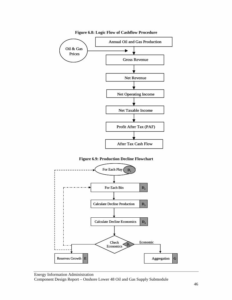
Figure 6.8: Logic Flow of Cashflow Procedure

Net Revenue

Net Operating Income

Net Taxable Income

Profit After Tax (PAF)

After Tax Cash Flow

Annual Oil and Gas Production

Gross Revenue

Oil & GasPrices

Net Revenue

Net Operating Income

Net Taxable Income

Profit After Tax (PAF)

After Tax Cash Flow

Annual Oil and Gas Production

Gross Revenue

Oil & GasPrices

Figure 6.9: Production Decline Flowchart

For Each Play

For Each Bin

Calculate Decline Production

Calculate Decline Economics

Check Economics

Reserves Growth Aggregation

D1

D2

D3

D4

E G

D5Economic

For Each Play

For Each Bin

Calculate Decline Production

Calculate Decline Economics

Check Economics

Reserves Growth Aggregation

D1

D2

D3

D4

E G

D5Economic


Reserves Growth Potential (E): The potential production of discovered resources through reserves growth in existing fields and reservoirs is calculated. In order to determine reserves growth from the discovered resource, pseudo-projects are created to perform a life-cycle economics on various processes. This is also done to mimic the way an operator will make decision to implement a recovery process in the field. As shown in Figure 6.5, the pseudo-projects are created from uneconomic wells (E1). These pseudo-projects are used to define the reserves growth projects (E2), which are evaluated for full life-cycle economics in step E3. The economic projects are then processed for development in step F for project ranking. Details of each step in calculating the reserves growth potential are further described in the following sections. Create pseudo-projects (E1): A pseudo-project of about 20 – 30 wells is created from the remaining uneconomic wells to calculate the full-cycle economics of various reserves growth processes. Well from uneconomic bins are selected using a random number generator. A pseudo-random methodology will be applied to the well selection to ensure that different runs, if the initial conditions are the same, will create the same pseudo-projects. The major steps are:

Step 1: Read in the number of uneconomic wells passed from step D. This is done for both oil and gas.

Step 2: Determine which bins cannot be combined into a pseudo-project. This is done according to the depth bin categories to ensure that incompatible projects, such as a combination of shallow and ultra-deep wells, are not formed.

Step 3: Create pseudo-projects using a pseudo-random well selection methodology. Each project has up to n wells, where n is a user specified value.

Step 4: Assign the play average properties to the pseudo-projects.

Step 5: Repeat steps 1 through 4 for each play with available wells.

Step 6: Pass the list of pseudo-projects on to E2 for the determination of reserve growth potential.

Define reserves growth (E2): The potential incremental production is determined, using the process-specific type curves, for each of the reserves growth projects created in E1. The resulting list of projects and their production profiles are then transferred to E3 for economic analysis. The major sub-steps are:

Step 1: Read the set of pseudo-projects for each play.

Step 2: Apply process screening criteria to the play average properties to determine the reserves growth processes which are applicable to the project.

Step 3: Use the process-specific type curve functions described in section 6.2.iii to determine the potential additional production for every applicable process.

Step 4: Repeat steps 2 and 3 for each pseudo project in each play.

Step 5: Pass the list of potential reserves growth projects on to E3 for economic calculation.


Reserves growth economics (E3): The economic viability of each potential reserves growth project defined in E2 is evaluated using the standard cashflow analysis previously described. The resulting list containing the potential projects and their economic calculations is then passed on to step F for project ranking. The major steps are:

Step 1: Read the list of reserves growth projects.

Step 2: Use the production profile, process-specific costs, and other economic parameters to perform the cashflow analysis of the project.

Step 3: Calculate the investment efficiency for each reserves growth project.

Step 4: Repeat steps 2 and 3 for each reserves growth project

Step 5: Pass the results on to step F for project ranking.

Project Ranking (F): The lists of potential exploration projects created in step C and the list of potential reserves growth projects created in step E are combined. The combined list is sorted by region and ranked by investment efficiency or probability of discovery. The ranked list is then passed on to step G for timing and aggregation. The major steps include:

Step 1: Read the lists of potential reserves growth and exploration projects.

Step 2: Incorporate any untimed economic projects from step G in the previous YEAR.

Step 3: Sort the list by region.

Step 4: Within each region, rank the projects by investment efficiency (reserves growth projects) or probability of discovery (exploration projects).

Step 5: Pass the sorted and ranked list to step G for timing and aggregation.

Timing and Aggregation (G): Timing and aggregation is the most important element of OLOGSS. In this module all decisions are made for future development: the potential reserves growth and exploration projects are selected on a regional basis and are timed subject to the development constraints. All technology levers and economic levers in the OLOGSS are embedded in the timing of any prospect. Figure 6.10 provides the logic flow of the timing and aggregation submodule of OLOGSS. Each step of this submodule is further described in detail on the following sections. Check Shut in (G1): Before evaluating reserves-growth potential, the shut-in status of pseudo projects created in previous years is examined. A shut-in project is a project that is abandoned because it has been uneconomic for a number of years under decline production and either no reserves-growth processes have been applied or they have been applied and their effectiveness has diminished. The number of years, called the “shut-in window” is a user-specified value. In the model, a project is shut in if the year of analysis equals the shut-in year.


Figure 6.10: Ranking and Selection Logic Flow

Rank Order Projects

Check Shut In

CheckConstraintsTag as Shut In

Run Economics Tag for

Development

Economic

Undeveloped

Economic Developed

Aggregation

Yes

Yes

No

No

F

G2

G3G5

G6

G7

G8

G1

G4

Rank Order Projects

Check Shut In



Development

Economic

Undeveloped

Economic Developed

Aggregation

Yes

Yes

No

No

F

G2

G3G5

G6

G7

G8

G1

G4

Rank Order Projects

Check Shut In



Development

Economic

Undeveloped

Economic Developed

Aggregation

Yes

Yes

No

No

F

G2

G3G5

G6

G7

G8

G1

G4

If the YEAR evaluated by OLOGSS is equal to shut_in_year for the project, the project is tagged for shut-in and passed to G2. Otherwise, the project is passed on to G4. Tag as Shut-in (G2): The project is tagged as “shut in” and passed on to step G3 where the economics will be run. Run Economics (G3): The costs for shutting in the project and associated environmental clean-up are calculated. These costs will be of the form:

)tcos_close,tcos_env(f)well/$K(shutin_tcos ii= Where: i = OLOGSS region env_cost = environmental clean-up costs close_cost = costs to close down the well cost_shutin = cost to shut in the project These costs are passed to step G6 for development and aggregation. Check Constraints (G4): Those projects that are not to be shut in are passed to this step. In this step, the regional development constraints are first examined. If there are sufficient development constraints, the project is passed on to step G5 to be tagged to be timed (developed). Otherwise it is passed on to step G8 to be tagged as untimed (undeveloped). The major steps include:


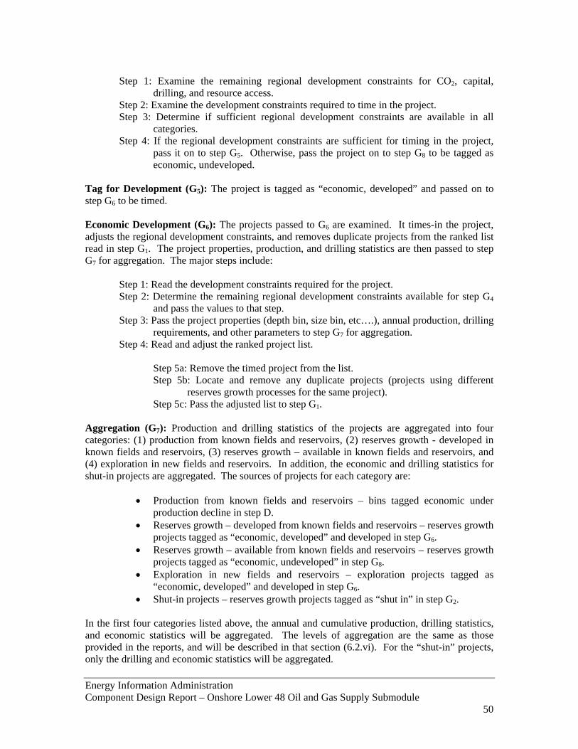
Step 1: Examine the remaining regional development constraints for CO2, capital, drilling, and resource access.

Step 2: Examine the development constraints required to time in the project. Step 3: Determine if sufficient regional development constraints are available in all

categories. Step 4: If the regional development constraints are sufficient for timing in the project,

pass it on to step G5. Otherwise, pass the project on to step G8 to be tagged as economic, undeveloped.

Tag for Development (G5): The project is tagged as “economic, developed” and passed on to step G6 to be timed. Economic Development (G6): The projects passed to G6 are examined. It times-in the project, adjusts the regional development constraints, and removes duplicate projects from the ranked list read in step G1. The project properties, production, and drilling statistics are then passed to step G7 for aggregation. The major steps include:

Step 1: Read the development constraints required for the project. Step 2: Determine the remaining regional development constraints available for step G4

and pass the values to that step. Step 3: Pass the project properties (depth bin, size bin, etc….), annual production, drilling

requirements, and other parameters to step G7 for aggregation. Step 4: Read and adjust the ranked project list.

Step 5a: Remove the timed project from the list. Step 5b: Locate and remove any duplicate projects (projects using different

reserves growth processes for the same project). Step 5c: Pass the adjusted list to step G1.

Aggregation (G7): Production and drilling statistics of the projects are aggregated into four categories: (1) production from known fields and reservoirs, (2) reserves growth - developed in known fields and reservoirs, (3) reserves growth – available in known fields and reservoirs, and (4) exploration in new fields and reservoirs. In addition, the economic and drilling statistics for shut-in projects are aggregated. The sources of projects for each category are:

• Production from known fields and reservoirs – bins tagged economic under production decline in step D.

• Reserves growth – developed from known fields and reservoirs – reserves growth projects tagged as “economic, developed” and developed in step G6.

• Reserves growth – available from known fields and reservoirs – reserves growth projects tagged as “economic, undeveloped” in step G8.

• Exploration in new fields and reservoirs – exploration projects tagged as “economic, developed” and developed in step G6.

• Shut-in projects – reserves growth projects tagged as “shut in” in step G2. In the first four categories listed above, the annual and cumulative production, drilling statistics, and economic statistics will be aggregated. The levels of aggregation are the same as those provided in the reports, and will be described in that section (6.2.vi). For the “shut-in” projects, only the drilling and economic statistics will be aggregated.


Economic Undeveloped (G8): Economic projects that cannot be developed in the current year due to insufficient development constraints are passed to this step. Projects are tagged as “economic, undeveloped”, and the shut-in window is created. The project is then passed on to step G7 for aggregation. The major steps include:

Step 1: Tag the project as “economic, undeveloped”. Step 2: If the project was created this year, tag the project with the year_created to

establish the shut-in window. Step 3: Remove the project from the ranked list and pass the list to step G1. Step 4: Pass the project to step G7.

Is it the Last Year (End of Year Loop): If the year of analysis is the last year of the model run, the year loop will be ended and the analysis will proceed to step H. Otherwise, it will return to step B. Reports (H): The reports transfer the annual and cumulative reports of the OLOGSS run to other OGSM submodules, other NEMS modules, and the user. The reports are provided at different geographical and resource-specific levels of disaggregation. These levels of disaggregation will be described in section 6.2.vi.

6.2.5. Modeling Impact of Technology Improvement Research and development programs are designed to improve technology to increase the amount of resources recovered from oil and gas fields. Key areas of study are: increasing production, extending reserves, and reducing costs. To optimize the impact of the R&D effort, potential benefits of a new technology are weighed against the costs of research and development. OLOGSS has the capability to model the effects of R&D programs and other technology improvements as they impact the production and economics of a project. This will be done in two steps: (1) modeling the implementation of the technology within the oil and gas industry and (2) modeling the costs and benefits for a project that applies this technology. Figure 6.11 illustrates the effects of the technology improvement on production and on project economics of a hypothetical well. The graphs plot the daily average production, projected by decline analysis, over the life of the project. Each graph represents a different scenario: (A) base case, (B) production improvement, and (C) economic improvement. Graph A plots the production for the base case. In the base case, no new technology is applied to the project. The end of the project’s economic life, the point at which the potential revenues are less than the costs of further production, is indicated. At that point, the project would be subject to reserves-growth processes or shut in. Graph B plots the production for the base case and a production-increasing technology such as skin reduction. The reduction in skin, through well-bore fracturing or acidizing, increases the daily production flow rate. This increased daily production rate is shown by the dotted line in graph B. The outcome of the production-increasing technology is reserves growth for the well. The amount of reserves growth for the well is shown by the area between the two lines as illustrated in figure 6.11 graph B.


Another example of technology improvement is captured in Graph C. In this case a technology is implemented that helps reduce the cost of operation and maintenance, thereby extending the reservoir life as shown in Figure 6.11 graph C.

Figure 6.11: Impact of Economic and Technology Levers

Time

Ave

rage

Dai

ly P

rodu

ctio

n (B

OE)

History Future

End of Economic Life

Time

Ave

rage

Dai

ly P

rodu

ctio

n (B

OE)

History Furture


I

Extended Life

II

C: Improvement of Project Economics

B: Improvement of Production

A: Base Case

Time

Ave

rage

Dai

ly P

rodu

ctio

n (B

OE)

History Future

Time

Ave

rage

Dai

ly P

rodu

ctio

n (B

OE)

History Future


Time

Ave

rage

Dai

ly P

rodu

ctio

n (B

OE)

History Furture


I

Extended Life

II

C: Improvement of Project Economics

B: Improvement of Production

A: Base Case

Time

Ave

rage

Dai

ly P

rodu

ctio

n (B

OE)

History Future

Technology improvements are modeled in OLOGSS using a variety of technology and economic levers. The technology levers, which impact production, are applied to the production type-curve functions. The economic levers, which model improvement in project economics, are applied to the cashflow calculations. Technology penetration curves are used to model the market penetration of each technology. The technology-penetration curve is divided into three sections, which each represent a phase of development. The first section is the Research and Development phase. In this phase the technology is developed and tested in the laboratory. During these years, the industry may be aware of the technology but has not begun implementation. The second section corresponds to the commercialization phase. In the commercialization phase, the technology has successfully left the laboratory and is being adopted by industry. The third section represents maximum market penetration. This is the ultimate extent to which the technology is adopted by industry. Figure 6.12 provides the graph of a generic technology-penetration curve. This graph plots the fraction of industry using the new technology (between 0 and 1) over time. During the research and development phase (A) the fraction of industry using the technology is 0. This increases during the commercialization phase (B) until it reaches the ultimate market penetration. In phase


C, the period of maximum market penetration, the percentage of the industry using the technology remains constant.

Figure 6.12: Generic Technology Penetration Curve

Ultimate Market Penetration

Time

Frac

tion

of In

dust

ry U

sing

Tec

hnol

ogy 1

0

A B C

Time

Frac

tion

of In

dust

ry U

sing

Tec

hnol

ogy 1

A B C

Ultimate Market Penetration

Time

Frac

tion

of In

dust

ry U

sing

Tec

hnol

ogy 1

0

A B C

Time

Frac

tion

of In

dust

ry U

sing

Tec

hnol

ogy 1

A B C

The success of the technology program is measured by estimating the probability that the technology development program will be successfully completed. It reflects the pace at which technology performance improves and the probability that the technology project will meet the program goals. There are four possible profiles: convex, concave, sigmoid/logistic, or linear, as shown in Figure 6.13. The convex curve corresponds to rapid initial penetration followed by slow penetration. The concave curve corresponds to slow initial penetration followed by rapid penetration. The sigmoid/ logistic curve represents a slow initial adoption rate followed by rapid increase in adoption and then slow adoption again as the market becomes saturated. The linear curve represents a constant rate of penetration, and may be used when no other predictions can be made. The market penetration curve is a function of the relative economic attractiveness of the technology instead of being a time-dependent function. A technology will not be implemented unless the benefits through increased production or cost reductions are greater than the cost to apply the technology. As a result, the market penetration curve provides a limiting value on commercialization instead of a specific penetration path. In addition to the curve, the implementation probability captures the fact that not all technologies that have been proved in the lab are able to be successfully implemented in the field. The implementation probability does not reflect resource access, development constraints, or economic factors.


Figure 6.13: Potential Market Penetration Profiles

0%

20%

40%

60%

80%

100%

logisticlinearconcaveconcave

0%

20%

40%

60%

80%

100%

logisticlinearconcaveconvex

0%

20%

40%

60%

80%

100%

logisticlinearconcaveconcave

0%

20%

40%

60%

80%

100%

logisticlinearconcaveconvex

The three phases of the technology penetration curve are modeled using three sets of equations. The first set of equations models the research and development phase, the second set models the commercialization phase, and the third set models the maximum market penetration phase. In summary, technology penetration curves are defined using the following variables:

• Number of years required to develop a technology = Yd • First year of commercialization = Yc • Number of years to fully penetrate the market = Ya • Ultimate market penetration ( %) = UP • Probability of success = Ps • Probability of Implementation = Pi • Percent of industry implementing the technology (fraction) in year x = Impx

1. Research and Development Phase: For years x < YsModeled using the equation:

00.pIm x = Where: x = year analyzed = percentage of industry implementing technology in year x xpIm This equation is used for all values of market_penetration_profile 2. Commercialization Phase: For years x >= Yc AND x < Yc + Ya – 1 The equations used to model this phase depend upon the value of market_penetration_profile If market_penetration_profile = convex


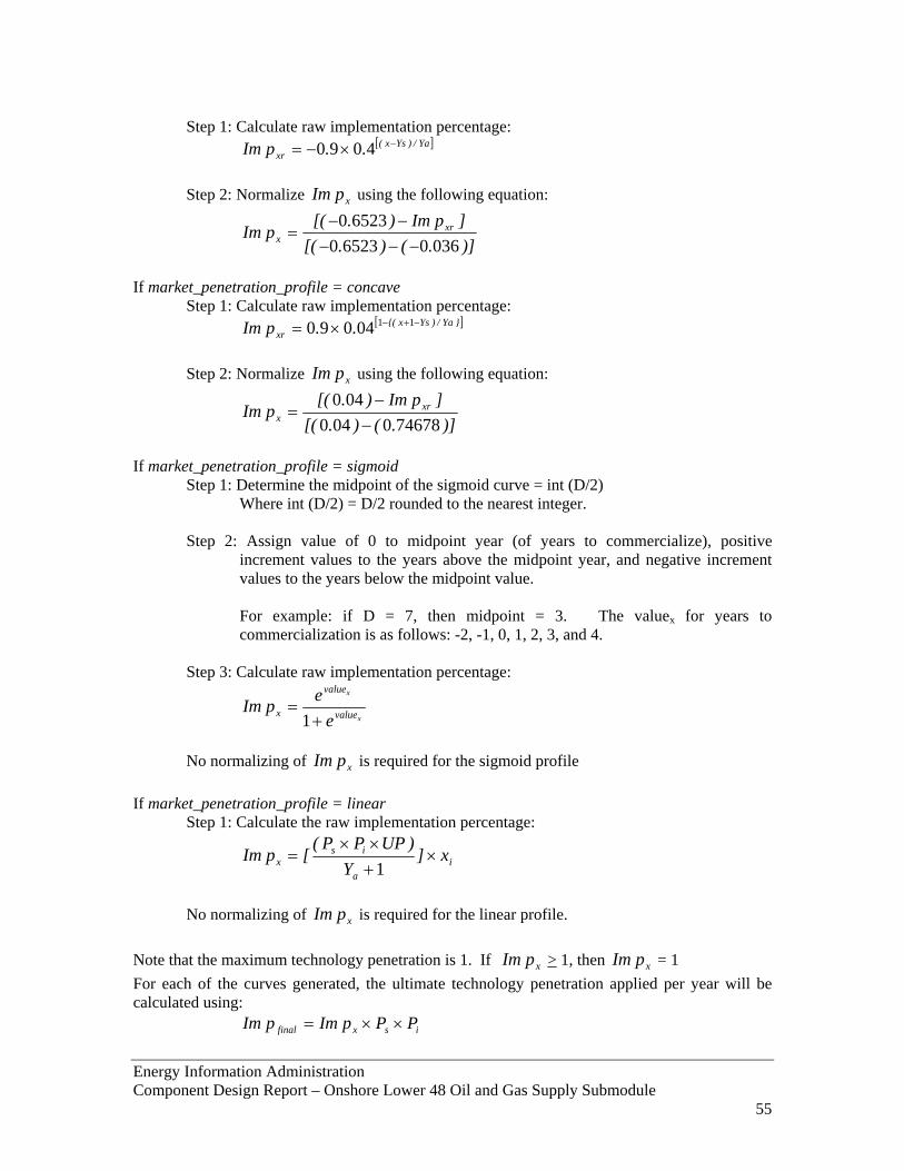
Step 1: Calculate raw implementation percentage: [ ]Ya/)Ysx(

xr ..pIm −×−= 4090 Step 2: Normalize using the following equation: xpIm

)].().[(]pIm).[(

pIm xrx 036065230

65230−−−

−−=

If market_penetration_profile = concave

Step 1: Calculate raw implementation percentage: [ ]}Ya/)Ysx{(

xr ..pIm −+−×= 1104090 Step 2: Normalize using the following equation: xpIm

)].().[(

]pIm).[(pIm xr

x 746780040040−−

=

If market_penetration_profile = sigmoid

Step 1: Determine the midpoint of the sigmoid curve = int (D/2) Where int (D/2) = D/2 rounded to the nearest integer.

Step 2: Assign value of 0 to midpoint year (of years to commercialize), positive

increment values to the years above the midpoint year, and negative increment values to the years below the midpoint value. For example: if D = 7, then midpoint = 3. The valuex for years to commercialization is as follows: -2, -1, 0, 1, 2, 3, and 4.

Step 3: Calculate raw implementation percentage:

x

x

value

value

x eepIm+

=1

No normalizing of is required for the sigmoid profile xpIm

If market_penetration_profile = linear Step 1: Calculate the raw implementation percentage:

ia

isx x]

Y)UPPP(

[pIm ×+××

=1

No normalizing of is required for the linear profile. xpIm Note that the maximum technology penetration is 1. If xpIm > 1, then = 1 xpImFor each of the curves generated, the ultimate technology penetration applied per year will be calculated using:

isxfinal PPpImpIm ××=


Note that is not to exceed Ultimate market penetration (“UP”) finalpIm 3. Maximum Market Penetration: For years >= Ys + Ya – 1 Modeled using the equation: finalx pImpIm = Where: x = year analyzed = percentage of industry implementing technology in year x xpIm This equation is used for all values of market_penetration_profile By using these three sets of equations, the industry-wide implementation of a technology improvement can be mapped using a technology-penetration curve.

As an example, suppose a new drill bit is developed which decreases the cost of drilling for all projects. This technology will take 5 years to develop and an additional 6 years to fully commercialize. The probability of R&D success is 80% and 75% of the industry is ultimately expected to implement the new drilling technology. The probability of implementation is 90%. The slope of the market penetration curve will be convex. The values of the variables in the technology penetration curve are: Yd = 5 Yc = 5 Ya = 6 UP = 0.75 Ps = 0.8 Pi = 0.9 x = year of analysis market_penetration_profile = convex These values will be used to solve for:

xpIm = Percent of industry implementing the technology (fraction) in year x. In the first section of the technology penetration curve, corresponding to years 1 to 5, the technology is being developed and is unavailable for industry adoption. The curve, between years 5 and 11, corresponds to the commercialization phase. The ultimate technology penetration is reached in year 11. The percentage reached at maximum market penetration at 54% of the industry. This value was calculated using:

isxfinal PPpImpIm ××= ,

Where: =UP. xpIm

Therefore, 5409080750 ....pIm Final =××=


The years between 11 and 20 correspond to the maximum market penetration. During this time, the penetration rate remains equal to . No additional adoption occurs during this phase of the penetration curve. The complete technology penetration curve generated by the equations for the three phases is shown in figure 6.14.

finalpIm

Figure 6.14: Technology Penetration Curve for New Drill Bit

0.00

0.10

0.20

0.30

0.40

0.50

0.60

1 2 3 4 5 6 7 8 9 10 11 12 13 14 15 16 17 18 19 20

Years

Prob

abili

ty o

f Im

plem

enta

tion

Annual Technology Penetration

Project Level Technology Impact: Adopting a new technology can impact two aspects of a project. It improves the production and/or improves the economics. Technology and economic levers are variables in the decline-curve or process-specific type curves (for technology), or in the economic module (for economics). The values for these levers are set by the user. Technology levers are identified when process-module type curves are developed; examples of such levers are presented in section 6.2.iii. Additional technology levers will be identified to represent future advancements in technology. There are two ways in which the economic levers are applied to the cashflow calculations: the cost to apply the technology and cost reductions. The cost to apply is the incremental cost to apply the technology. The cost reduction is the savings associated with using the new technology. Each type of cost is modeled using economic levers. The cost-reduction costs model the savings brought about through technology improvement. By using both types of levers, the synergy between additional costs and offsetting cost reductions can be captured.

As an example, suppose an acidizing technique will be applied to improve the production flow rate by decreasing the skin. The improvement in production is modeled using the PI lever. The impact on project economics is modeled using the skin_cost and skin_apply levers. Setting the PI lever to 5 will model a 5% increase in the productivity index and results in an increase in the daily


production flow rate. By setting the skin_apply lever to 10 (K$), the cost to apply the technology is modeled in the economic calculations. Setting the skin_cost lever to 3 reduces stimulation costs by 3%. The cost to apply is offset by the cost savings and the increased revenues caused by the improved daily production. The result is an improvement in the project economics and a potential extension of the project lifespan.

The technology will be implemented by the model only if the cost to apply the technology is less than the increased revenue generated by improved production and by cost reductions. The specific economic levers will be identified, as with the technology levers, during a review of the process models. Resource and Filter levers: Two other types of levers will be incorporated into OLOGSS: resource-access levers and filter levers. Resource-access levers allow the user to model changes in resource-access policy. The filter levers allow the technology, economic, and resource-access levers to be applied to different geographical and resource categories. These categories include: region, play, depth category, and other levels at which economic and production analyses occur. In summary, the OLOGSS is capable of modeling the impact of R&D programs and other technology improvements. The implementation of a new technology throughout the industry is quantified and modeled using a technology-penetration curve. The penetration curve incorporates the three phases of implementation: development, commercialization, and maximum market penetration. For modeling technology improvements on the project level, levers are applied that capture the improvements in production, the costs to apply the technology, and the associated cost reductions. Resource-access levers, allowing the analysis of resource-access issues, are incorporated into OLOGSS. Filter levers, which allow the target of other levers to be specified, will also be incorporated into the model. Additional types of levers may be identified and incorporated.

6.2.6. Reporting Module The reporting module passes the results of the OLOGSS run on to other OGSM submodules, NEMS modules, and the user. This is done on an annual and cumulative basis. There are three broad categories of reports: (1) supply, (2) drilling, and (3) economic. The reported results and levels of disaggregation for each category are discussed in this section. Supply: Supply reports provide annual and cumulative oil and gas supply, at given oil and gas prices, in the following sub-categories: • Production in existing fields and reservoirs • Production from reserves growth – developed in existing fields and reservoirs • Production from reserves growth – available in existing fields and reservoirs but not yet

developed using a reserves-growth process • Production from exploration in new fields and reservoirs


Drilling: Drilling reports present the annual and cumulative drilling constraints available and used during the development of the oil and gas projects. They will provide drilling statistics in the following sub-categories: • Number of projects drilled • Developmental footage drilled • Exploratory footage drilled • Capital used • CO2 used • Other development constraints used • Other reports to be determined

Economic: Economic reports provide the economic statistics for the projects developed. These reports are based upon the cashflow analyses of the developed projects. Reports within this category include: • Capital investments and costs • Operating costs • Federal and state income taxes • Transfer payments (Federal royalty and state severance taxes) • Environmental Costs • Tax Credits • Other reports to be identified

Disaggregation: The reports will be generated at the following levels of disaggregation (where applicable): • OGSM region • PMM region • NGTDM region • State • Basin • Play • Depth bin category • Size category • Crude oil • Non-associated gas • Associated dissolved gas • Conventional or unconventional resources • Known Fields or undiscovered resources • Source of production:

o Known fields and reservoirs o Reserves growth processes in known fields and reservoirs o Exploration in new fields and reservoirs

Other levels of disaggregation may be identified and included.


7. Uncertainty and Limitations Important assumptions and limitations to the OLOGSS design are summarized as follows:

7.1. Assumptions In developing the methodology for the OLOGSS, assumptions were made about the resources modeled, the decline-curve analysis, and the process-specific type curves.

• Resource modeled: The primary assumption about the resource is that the geological and petrophysical properties can be captured by play-level averages. It is assumed that the variations within the play are negligible and thus can be ignored.

• Decline curve analysis: It is assumed that the production for wells in existing fields and

reservoirs can be forecast using averaged historical data. It is assumed that the variations within the historical data, when grouped into the well bins, would result in minor variations, small enough to ignore, in the production from that bin.

• Process specific type curve: The process-specific type curves are generated using

prototypical reservoirs, key variables, and orthogonal experiments developed using a simulator. As the type curve will incorporate a limited number of play-level properties, it is assumed that the incorporated variables provide all significant contributions to production. Therefore the variables not incorporated into the equations can be ignored.

7.2. Limitation of Model The limitations of the model are caused by the selection of the unit of analysis. As OLOGSS is a play-level model, the play is the smallest geographical/ geographical structure at which analysis is conducted. This decision, made because of the regularly availability of play-level data and a targeted short execution time, has the following consequences:

• Loss of specific reservoir and fields properties: OLOGSS uses play average properties and average historical data. These are used in forecasting reserves growth and production in existing fields and reservoirs. The model does not have reservoir-specific historical data or properties to predict the exact production from reservoirs.

• Inability to capture variations within the play: The use of play-level average

properties does not allow the petrophysical or geologic variations within the play to be captured or modeled. This affects the modeling of reserves growth, which is done using the average properties. The result is that a reserves growth project will forecast average production.

• Inability to precisely locate the source of production: In interpreting the forecast

production, the exact geographic source of the production cannot be determined. As the play is the unit of analysis, and the bin classification does not capture the physical


location of the wells, it is not possible to determine the source of production below that level. Thus OLOGSS cannot be used for analysis at any level finer than the play.

• Inability to exactly target technology and economic levers: As the analysis is done at

the play level, technology and economic levers cannot be targeted to specific fields, reservoirs, or wells. The lack of detailed reservoir or field properties prevents the filter levers from being applied to a unit smaller than the well bin. This is the smallest level at which technology or economic policy can be modeled.

None of the above limitations invalidate the model and its analyses if they are viewed as they are intended, which is an estimate of the potential oil and gas supply from the Lower 48 onshore.


8. Conclusions and Recommendations This component design report describes the features and methodology of the new Onshore Lower 48 Oil and Gas Supply Submodule. The OLOGSS was designed to replace these submodules within NEMS and enhance the modeling capabilities of the system through incorporation of technology, economic, resource access, and other types of model levers.

8.1. Conclusions The OLOGSS is an oil and gas supply model which will replace the onshore lower 48 component of the OGSM. It has the following key characteristics:

• It models oil and gas, discovered and undiscovered, for conventional and unconventional resources.

• It forecasts production from known fields and reservoirs, as well as reserves growth in known fields and reservoirs at the play level.

• It forecasts exploration in new fields and reservoirs at the cell/accumulation level, and aggregates these to the play level.

• It uses process-specific type curves to forecast reserves growth.

• It uses resource/process-specific capital, operating, and other cost parameters to conduct economic analysis using a standard cashflow procedure

• It mimics the method industry uses to make development decisions by selecting projects based upon economic efficiency and the regional availability of development constraints.

• It reports annual and cumulative production, drilling statistics, and economic statistics using resource categories and levels of disaggregation based upon geography and resource properties.

• It has seven regions based upon the OGSM regions selected to maintain continuity with the historical data and to allow easy transfer of results to OGSM, PMM, NGTDM, and other NEMS modules.

• It has sufficient technology levers for analyzing the impacts of R&D programs on oil and gas production.

• It has sufficient economic and tax levers for analyzing the impact of economic and policy changes on oil and gas production.

8.2. Recommendations It is recommended that the methodology described in this document be subjected to a peer review by the Energy Information Administration and the customers whose needs will be met using the model. Suggestions from the peer review should be captured and incorporated into the National Energy Modeling System. Energy Information Administration Component Design Report – Onshore Lower 48 Oil and Gas Supply Submodule 62

9. References

1. U.S. Department of Energy. 2005. Documentation of the Oil and Gas Supply Submodule (OGSM), DOE/EIA – M063 (2005), Energy Information Administration, Washington, DC.

2. U.S. Department of Energy. 2003. The National Energy Modeling System: An Overview 2003, DOE/EIA-0581(2003), Energy Information Administration, Washington, DC.

3. U.S. Department of Energy. 2005. Natural Gas Transmission and Distribution Module of the National Energy Modeling System, DOE/EIA-M062, Energy Information Administration, Washington, DC.

4. U.S. Department of Energy. 2005. Petroleum Market Model of the National Energy Modeling System, Part 1 – Report and Appendix A, DOE/EIA-M059 (2005) Part 1, Energy Information Administration, Washington, DC.

5. U.S. Department of Energy. 2005. Documentation of the Oil and Gas Supply Submodule (OGSM), DOE/EIA – M063 (2005), Energy Information Administration, Washington, DC. Page 2-1.

6. U.S. Department of Energy. Component Design Report, Basic Framework & Onshore Lower 48 Conventional Oil and Gas Supply, Energy Information Administration, Washington, DC. Page 7.

7. Donald L. Gautier and others, U.S. Department of Interior, U.S. Geological Survey, 1995 National Assessment of the United States Oil and Gas Resources, (Washington, D.C., 1995); U.S. Department of Interior, Minerals Management Service, an Assessment of the Undiscovered Hydrocarbon Potential of the Nation’s Outer Continental Shelf, OGS Report MMS 96-0034 (June 1996); and 2003 estimates of conventionally recoverable hydrocarbon resources of the Gulf of Mexico and Atlantic Outer Continental Shelf as of January 1, 2003.

8. U.S. Department of Energy. 2000. Costs and Indices for Domestic Oil and Gas Field Equipment and Production Operations DOE/EIA-0185(2000). Energy Information Administration, Washington, D.C.

9. American Petroleum Institute. 2005. 2003 Joint Association Survey on Drilling Costs. Washington, D.C.

10. U.S. Department of Energy. 2005. Documentation of the Oil and Gas Supply Submodule (OGSM), DOE/EIA – M063 (2005), Energy Information Administration, Washington, DC. Page 3-B-11.

11. U.S. Department of Energy. 2003. Integration of the NETL Oil & Gas Modeling Systems –Reservoir Description Module, National Energy Technology Laboratory, Washington, D.C., page 61

12. HPDI, 2006. Historical Production Data

13. American Petroleum Institute. 2005. 2003 Joint Association Survey on Drilling Costs. Washington, D.C.

14. Publications of the Society of Petroleum Engineers

15. Publications of the Gas Technology Institute


16. U.S. Department of Energy. 2005. Oil and Gas Lease Equipment and Operating Costs 1987 Through 2004. Energy Information Administration, Washington, D.C.





21. National Petroleum Council, 1984. Enhanced Oil Recovery. Washington, D.C.


23. Department of the Treasury, Internal Revenue Service

24. Independent Petroleum Association of America. 2000. The Oil and Gas Producing Industry in Your State. Washington, D.C.

25. U.S. Department of Energy. 2005. Performance Profiles of Major Energy Producers 2003, DOE/EIA-0206(05) Distribution Category UC-950. Energy Information Administration, Washington, D.C


Documents

Onshore Lower 48 Oil and Gas Supply Submodule Coponent ... · PDF fileStatement of Purpose ... Summary of Models Reviewed ... Onshore Lower 48 Oil and Gas Supply Submodule Coponent