Online Trajectory Planning in DynamicEnvironments for Surgical Task Automation

Takayuki Osa, Naohiko Sugita, and Mitsuishi MamoruDepartment of Mechanical Engineering, The University of Tokyo, Japan

Email: {osa, sugi, mamoru}@nml.t.u-tokyo.ac.jp

Abstract—Automation of robotic surgery has the potential toimprove the performance of surgeons and the quality of thelife of patients. However, the automation of surgical tasks haschallenging problems that must be resolved. One such problemis adaptive online trajectory planning based on the state of thesurrounding dynamic environment. This study presents a frame-work for online trajectory planning in a dynamic environment forautomatic assistance in robotic surgery. In the proposed system,a demonstration under various states of the environment is usedfor learning. The distribution of the demonstrated trajectoryover the environmental conditions is modeled using a statisticalmodel. The trajectory, under given environmental conditions,is computed as a conditional expectation using the learnedmodel. Because of its low computational cost, the proposedscheme is able to generalize and plan a trajectory online in adynamic environment. To design the motion of the system totrack the planned trajectory in a stable and smooth manner, theconcept of a sliding mode control was employed; its stability wasproved theoretically. The proposed scheme was implemented on arobotic surgical system and the performance was verified throughexperiments and simulations. These experiments and simulationsverified that the developed system successfully planned andupdated the trajectories of the learned tasks in response to thechanges in the dynamic environment.

I. INTRODUCTION

As the clinical performance of robotic surgery has demon-strated, it will become a common procedure. For instance,the da Vinci system (Intuitive Surgical Inc., CA, US) hasproved its performance in many clinical studies and is installedin thousands of hospitals worldwide [5]. However, roboticsurgery still has significant potential to improve its clinicalperformance. Many studies have been conducted to developmore intelligent and sophisticated robotic surgical systems toimprove the quality of robotic surgery.

One of the research topics in this area is surgical taskautomation. It is believed that automatic assistance by a roboticsystem in a surgical operation would reduce a surgeon’s fatigueand operation time. However, the automation of surgical taskshas challenging problems that need to be resolved. One ofthese is the adaptation of the trajectory according to the stateof the dynamic environment.

In surgical task automation, the robotic surgical system isexpected to cooperate with surgeons and work with flexibleand movable objects such as threads, needles, and soft tissues.Therefore, the robotic system must adapt its motion accordingto the motion of the surgeon, surgical instruments, and targetorgan.

Fig. 1. Surgical knot tying involves making loops around a surgicalinstrument. If the surgical instrument moves during the process, the trajectorymust be adapted online.

For example, surgical knot tying involves making loopsaround a surgical instrument using a thread held by anotherinstrument. In this looping task, the trajectories for makingthe loop must be adapted according to the position of thesurgical instrument, maintaining the topological feature of thetrajectory (Fig. 1). If the surgical instrument to be looped ismoving during the task, the trajectory must be recalculated andadapted online according to the motion. This kind of adaptivetrajectory planning is required for automatic assistance inmany situations. However, this online planning and adaptationof the trajectory is very challenging, and the solution for thisproblem has not yet been established.

In this paper, we present a method for learning time-andspace-dependent trajectories from demonstrations, and plan-ning and updating trajectories online adapting to changes in thedynamic environment. In the proposed scheme, demonstrationtrajectories, under various environmental conditions, are usedfor learning the task trajectory process. The demonstratedtrajectories are normalized in a time domain, and their dis-tribution over the environmental condition is modeled usinga statistical method. Using the learned models, the learnedtasks are generalized to the new state of the environment.Because of its low computational cost, this method is ableto plan and update trajectories online adapting to changesin the environment. On the other hand, the update of theplanned trajectories can also cause a discontinuous change ofthe planned trajectory. If the planned trajectory is input to thesystem directly, the discontinuous change could cause unstablesystem behavior. Therefore, we present a scheme to design the

motion of the slave manipulator to track the planned trajectoryin a smooth and stable fashion using the concept of a slidingmode control. The proposed scheme was implemented on arobotic surgical system and the performance of the developedsystem was verified through experiments and simulations.

This paper is structured as follows. The next section de-scribes the previous studies related to trajectory planning bylearning from demonstrations. Section III describes the detailsof the proposed method. Section IV provides the experimentsand simulations to evaluate the developed system. Section Vdiscusses the results presented in this study. The conclusionsand outline of future work can be found in Section VI.

II. RELATED STUDIES

Many studies related to the automation of surgical taskshave been published [19, 9, 10, 11]. However, to the bestof our knowledge, no existing surgical robotic system plansand updates a trajectory online to adapt to changes in theenvironment. Van der Berg et al. developed a system thatlearns surgical knot tying from demonstrations and executesthe learned task faster than the demonstrations [19]. However,the system cannot adapt the planned trajectory if the initialconditions change. Mayer et al. proposed approaches to learnsurgical tasks from demonstrations [9, 10, 11]. Although ascheme for generalizing the learned task to a new situationis presented in [10], the scheme cannot be applied to onlinetrajectory planning because of its computational costs andlimitations in modeling the situation for simulations. Schul-man et al. [16, 17] presented the most related works. Theyproposed a scheme to generalize demonstrated trajectories toa new situation, and they achieved automatic suturing in newsituations in a simplified setup [16]. However, it is expectedthat the computational cost will be considerably high for onlinetrajectory planning in a dynamic environment.

In the field of motion planning, the programming bydemonstration (PbD) approach has been investigated by manyresearchers [1]. One notable scheme is the movement primitiveapproach proposed by Schaal et al. [15, 12]. They achievedgeneralizing task trajectories to various start and end-points bylearning from demonstrations. However, this is not applicableto tasks where the topological features of the trajectory mustbe adapted according to the state of the environment. Anotherimportant previous work is presented by Billard et al. [7, 6, 4].They developed a scheme of learning tasks as a time-invariantdynamic system and adapting the motion trajectory in real-time for obstacle avoidance [6]. However, this scheme isnot applicable to time-dependent trajectories that are oftennecessary for surgical task automation.

In this paper, we present a system that learns time-andspace-dependent trajectories from demonstrations in variousenvironmental conditions and plans a trajectory online in thedynamic environment. In addition, this study presents a controlscheme to allow the system to track the planned and updatedtrajectories online, in a stable manner. The combination of theproposed trajectory-planning and trajectory-tracking schemes

(a) (b)

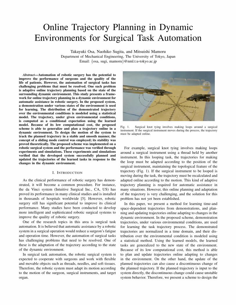
Fig. 2. Robotic telesurgery system: (a) slave and (b) master sites

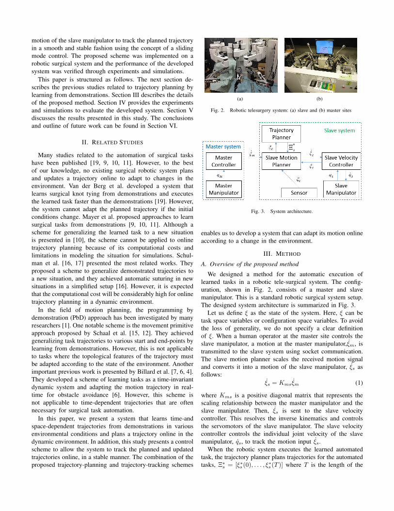
Fig. 3. System architecture.

enables us to develop a system that can adapt its motion onlineaccording to a change in the environment.

III. METHOD

A. Overview of the proposed method

We designed a method for the automatic execution oflearned tasks in a robotic tele-surgical system. The config-uration, shown in Fig. 2, consists of a master and slavemanipulator. This is a standard robotic surgical system setup.The designed system architecture is summarized in Fig. 3.

Let us define ξ as the state of the system. Here, ξ can betask space variables or configuration space variables. To avoidthe loss of generality, we do not specify a clear definitionof ξ. When a human operator at the master site controls theslave manipulator, a motion at the master manipulator,ξm, istransmitted to the slave system using socket communication.The slave motion planner scales the received motion signaland converts it into a motion of the slave manipulator, ξs asfollows:

ξs = Kmsξm (1)

where Kms is a positive diagonal matrix that represents thescaling relationship between the master manipulator and theslave manipulator. Then, ξs is sent to the slave velocitycontroller. This resolves the inverse kinematics and controlsthe servomotors of the slave manipulator. The slave velocitycontroller controls the individual joint velocity of the slavemanipulator, qs, to track the motion input ξs.

When the robotic system executes the learned automatedtask, the trajectory planner plans trajectories for the automatedtasks, Ξ∗

s = [ξ∗s (0), . . . , ξ∗s (T )] where T is the length of the

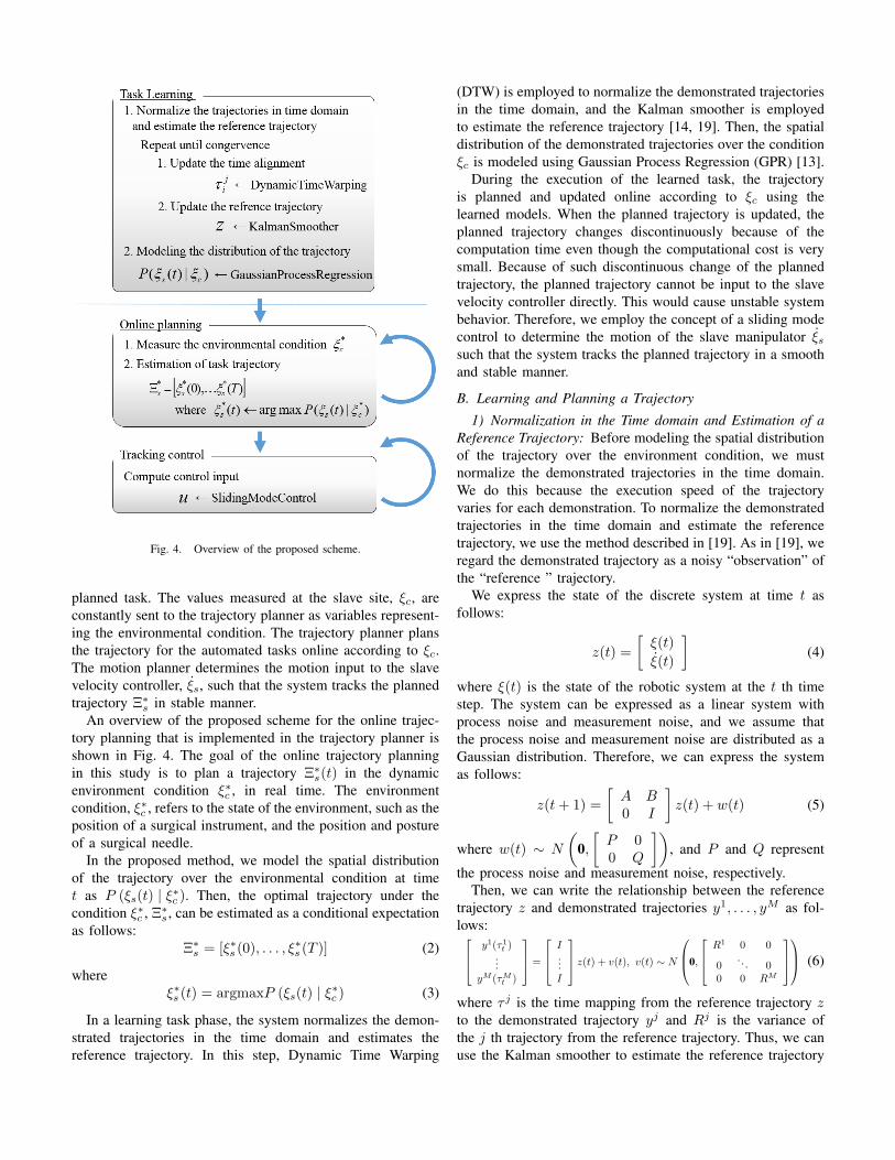
Fig. 4. Overview of the proposed scheme.

planned task. The values measured at the slave site, ξc, areconstantly sent to the trajectory planner as variables represent-ing the environmental condition. The trajectory planner plansthe trajectory for the automated tasks online according to ξc.The motion planner determines the motion input to the slavevelocity controller, ξs, such that the system tracks the plannedtrajectory Ξ∗

s in stable manner.An overview of the proposed scheme for the online trajec-

tory planning that is implemented in the trajectory planner isshown in Fig. 4. The goal of the online trajectory planningin this study is to plan a trajectory Ξ∗

s(t) in the dynamicenvironment condition ξ∗c , in real time. The environmentcondition, ξ∗c , refers to the state of the environment, such as theposition of a surgical instrument, and the position and postureof a surgical needle.

In the proposed method, we model the spatial distributionof the trajectory over the environmental condition at timet as P (ξs(t) | ξ∗c ). Then, the optimal trajectory under thecondition ξ∗c , Ξ∗

s , can be estimated as a conditional expectationas follows:

Ξ∗s = [ξ∗s (0), . . . , ξ∗s (T )] (2)

whereξ∗s (t) = argmaxP (ξs(t) | ξ∗c ) (3)

In a learning task phase, the system normalizes the demon-strated trajectories in the time domain and estimates thereference trajectory. In this step, Dynamic Time Warping

(DTW) is employed to normalize the demonstrated trajectoriesin the time domain, and the Kalman smoother is employedto estimate the reference trajectory [14, 19]. Then, the spatialdistribution of the demonstrated trajectories over the conditionξc is modeled using Gaussian Process Regression (GPR) [13].

During the execution of the learned task, the trajectoryis planned and updated online according to ξc using thelearned models. When the planned trajectory is updated, theplanned trajectory changes discontinuously because of thecomputation time even though the computational cost is verysmall. Because of such discontinuous change of the plannedtrajectory, the planned trajectory cannot be input to the slavevelocity controller directly. This would cause unstable systembehavior. Therefore, we employ the concept of a sliding modecontrol to determine the motion of the slave manipulator ξssuch that the system tracks the planned trajectory in a smoothand stable manner.

B. Learning and Planning a Trajectory

1) Normalization in the Time domain and Estimation of aReference Trajectory: Before modeling the spatial distributionof the trajectory over the environment condition, we mustnormalize the demonstrated trajectories in the time domain.We do this because the execution speed of the trajectoryvaries for each demonstration. To normalize the demonstratedtrajectories in the time domain and estimate the referencetrajectory, we use the method described in [19]. As in [19], weregard the demonstrated trajectory as a noisy “observation” ofthe “reference ” trajectory.

We express the state of the discrete system at time t asfollows:

z(t) =

[ξ(t)

ξ(t)

](4)

where ξ(t) is the state of the robotic system at the t th timestep. The system can be expressed as a linear system withprocess noise and measurement noise, and we assume thatthe process noise and measurement noise are distributed as aGaussian distribution. Therefore, we can express the systemas follows:

z(t+ 1) =

[A B0 I

]z(t) + w(t) (5)

where w(t) ∼ N

(0,[P 00 Q

]), and P and Q represent

the process noise and measurement noise, respectively.Then, we can write the relationship between the reference

trajectory z and demonstrated trajectories y1, . . . , yM as fol-lows: y1(τ1t )

...yM (τMt )

=

I...I

z(t) + v(t), v(t) ∼ N

0,

R1 0 0

0. . . 0

0 0 RM

(6)

where τ j is the time mapping from the reference trajectory zto the demonstrated trajectory yj and Rj is the variance ofthe j th trajectory from the reference trajectory. Thus, we canuse the Kalman smoother to estimate the reference trajectory

z. In (6), we set Rj = I for t = 0, . . . ,M so that all ofthe demonstrations contribute equally to the estimation of thereference trajectory.

To estimate the reference trajectory at the initial step, weinitialized the time alignment τ as follows:

τ jt =t

NT j (7)

where τ jt is the time alignment of the tth step of the jthdemonstration, N is the total number of time steps of thereference trajectory, and T j is the length of the jth demon-stration.

Then, the time alignment τ jt is updated for t = 0, . . . , Nand j = 0, . . . ,M with DTW using the reference trajectoryas the norm in the time domain [14]. In DTW, we employ thefollowing constraint for the time alignment:

1

2

(τoldt+1 − τoldt

)≤ τupdatet+1 − τupdatet ≤ 2

(τoldt+1 − τoldt

)(8)

where τoldt is the time alignment before the update and τupdatet

is the updated time alignment. This constraint means that theDTW changes the speed of the motion between half-speedand double-speed compared with the speed before the DTWprocess. This constraint avoids computing an unnatural timealignment.

After the time alignment is updated, the reference trajectoryis also updated using the updated time alignment. In thisprocessing loop, the updating of the time alignment andreference trajectory is repeated until the reference trajectoryconverges. In our cases, this loop was repeated once or twiceuntil convergence.

2) Modeling the distribution of the trajectories over theenvironmental condition: Using the trajectories normalizedin the time domain, we model the spatial distribution of thetrajectory over the environment condition. For this purpose,we employ GPR [13]. GPR is a non-parametric method forregression. It models a joint distribution of the data withoutdirectly modeling a regression function. Although there areother options for regression, such as Gaussian Mixture Re-gression [2, 7] and Locally Weighted Regression [3], we choseGPR because it can regress the nonlinear relationship globallyusing relatively little training data. We express the dataset ofthe demonstrations and the given environmental conditions asfollows:

X =

(ξ1c)T

...(ξMc)T

, Y =

(ξ1s (τ1i )− z(i)

)T...(

ξMs (τMi )− z(i))T

,X∗ =

[(ξ∗c )

T], Y ∗ =

[(ξ∗s (i)− z(i))T

](9)

where X is the set of the environmental conditions in thedemonstrations, Y is the set of deviations of the demonstratedtrajectories from the reference trajectory at the tth step, X∗

is the new environmental condition given for a trajectory esti-mation, and Y ∗ is the estimated deviation from the referencetrajectory under the environmental condition X∗ as the tth

step. In GPR, the distribution of Y can be modeled as a multi-variate as follows:

P

(yjy∗j

)∼ N

(0,

[K(X,X) + σ2

nI K(X,X∗)K(X∗, X) K(X∗, X∗) + σ2

nI

])(10)

where Y = [y1, . . . , yn] and K is the kernel matrix defined asfollows:

K(X,X) ∈ RM×M , (K(X,X))i,j = k(ξic, ξjc)

K(X∗, X) ∈ R1×M , (K(X∗, X))1,j = k(ξ∗c , ξjc)

K(X,X∗) ∈ RM×1, (K(X,X∗))i,1 = k(ξic, ξ∗c )

K(X∗, X∗) ∈ R, K(X∗, X∗) = k(ξ∗c , ξ∗c ) (11)

In (11), k(xi, xj) represents the kernel function. In the de-veloped system, we employ the squared exponential kernelfunction defined as [13]:

k(xi, xj) = σf exp

(− 1

2l2(xi − xj)T (xi − xj)

)(12)

The performance of the GPR depends on the selection ofthe hyperparameters [σf , σn, l]. These hyperparameters can beobtained by maximizing the marginal likelihood defined asfollows:

log p = −1

2yTKy − log det |K| − n log 2π (13)

The optimization problem of maximizing the marginal likeli-hood can be solved using gradient-based optimization meth-ods. This optimization problem often falls into local optima,and therefore, we perform the optimization from randomlychosen initial conditions to find the optimal hyperparameters.The hyperparameters are dependent on the training dataset,namely, X and Y , and are not dependent on the new en-vironmental condition X∗. Thus, the optimization of thehyperparameters is performed only before the execution ofthe task.

The joint distribution of the trajectory under the given envi-ronmental condition can be modeled as a Gaussian distributionas follows:

y∗j |yj , X,X∗ ∼ N (µ∗,Σ∗) (14)

where

µ∗ = K(X∗, X)(K(X,X) + σ2nI)−1yj (15)

Σ∗ = K(X∗, X∗) + σ2nI

− K(X∗, X)(K(X,X) + σ2nI)−1K(X,X∗) (16)

Therefore, the trajectory under the given environmental con-dition can be estimated as follows:

ξ∗s (t) = z(t) + argmaxP (Y ∗|Y,X,X∗)

= z(t) +(K(X∗, X)(K(X,X) + σ2

nI)−1Y

)T(17)

where ξ∗s (t) is the state of the system at the tth step in theestimated trajectory for the given environmental condition. Thecomplete trajectory Ξ∗ = [ξ∗s (0), . . . , ξ∗s (N)] can be obtainedby computing (17) for i = 0, . . . , N .

In this scheme, once K(X,X) and σn are obtained inthe offline phase, the only computation required for online

trajectory planning is computing (17) for i = 0, . . . , N , whichis a matrix calculation with relatively small computationalcost. This feature enables a trajectory planning in a dynamicenvironment with sufficiently short computation time.

C. Motion Control Scheme

When the planned trajectory is updated during the automa-tion task, it changes discontinuously. However, if the motioninput to the slave manipulator changes discontinuously, itcould cause unstable system behavior. Therefore, the motioninput to the slave manipulator must be designed to be smoothto ensure that the system tracks the updated trajectory in stablemanner.

For this purpose, we employ the concept of sliding modecontrol [18]. In this case, the control input to the system is thevelocity of the system. Therefore, the system can be expressedby a linear system as follows:

ξs = u (18)

In the framework of the sliding mode control, the desiredsystem behavior is expressed as a sliding surface as follows:

s(t) = ξs(t)− ξ∗s (t) = 0 (19)

where ξs(t) is the state of the system at time t and ξ∗s (t) isthe desired state at time t obtained from the updated plannedtrajectory.

We must design the motion input, u, so that the systemrobustly slides on the sliding surface. In this system, weemploy the following control law:

u(t) = u−K · sat (s(t))

= ξ∗s −K · sat (ξs(t)− ξ∗s (t)) (20)

where K =

k1 0 0

0. . . 0

0 0 kn

and ki > 0 for i = 1, . . . , n.

The saturation function sat(s) is expressed as follows:

sat(s) =

sat(s1). . .

sat(sn)

(21)

where

sat(si) =

1 (si > ci)si/ci (|s| < |ci|)−1 (si < −ci)

(22)

where ci is a positive constant value. In (20 ), the first termrepresents the control input to make the system slide on thesliding surface; the second term represents the control inputto make the system converge on the sliding surface. The useof the saturation function sat (x) is a common solution toavoid a “chattering” problem common to the sliding modecontrol. Furthermore, the control input defined as (20) isupper-bounded; it avoids excessive change of the controlinputs that could cause unstable system behavior.

In the framework of the sliding mode control, it is knownthat the system converges to the sliding surface in a finite

time if the following inequality is satisfied for a certain η =[η0, . . . , ηn]:

1

2

d

dts2i < −ηi |si| (23)

where s = [s0, . . . , sn]T = [ξ0 − ξ∗0 , . . . , ξn − ξ∗n]T and n isthe dimension of the system [18].

For the range of |si| > ci, the condition in (23) can bebriefly proved as described below. From (19) - (20), we canobtain the following equations.

1

2

d

dts2i = si · si

=(ξs,i(t)− ξ∗s,i(t)

)si

=(u(t)− ξ∗s,i(t)

)ss,i

= −ki(ξs,i(t)− ξ∗s,i(t)

)si

= −ki |si| (24)

From line 3 to line 5, we use (20). Therefore, using the controllaw in (20), the condition in (23) is satisfied, and the systemconverges to the neighbor of the updated trajectory in a finitetime.

Meanwhile, in the range of |si| > ci, the following condi-tion is satisfied:

si = ξs,i − ξ∗s,i= u− ξ∗s,i (25)= −kisat(si) (26)= −kisi (27)

Thus, the system exponentially converges to the sliding surfacein the neighborhood of the sliding surface. Therefore, itconverges from any state to the desired trajectory in a finitetime and tracks in stable manner using the control law in (20).

IV. EXPERIMENTS AND SIMULATIONS

The proposed scheme was implemented on the robotic sys-tem for remote surgery shown in Fig. 2. In the robotic system,two robotic surgical instruments are attached to two roboticarms; one laparoscope is attached to another robotic arm. Weperformed the experiments and simulations to evaluate the pro-posed scheme. In the experiments and simulations, the systemlearned two tasks, namely, a DOUBLE LOOP task and a PICKAND PULL task. Seven demonstrations were performed foreach of the tasks under various environmental conditions. Theenvironmental conditions were static during a demonstration.In the simulation, the demonstrated trajectories were separatedinto six demonstrations as a training dataset and one demon-stration for the validation data. The demonstration used forthe validation data had a different environmental conditionfrom that of the training dataset, and trajectories demonstratedand planned in the same environmental condition were com-pared. To quantify the correctness and smoothness of theplanned trajectories, the RMS error between the demonstratedtrajectory and the planned trajectory, 1/T

∑∥∥ξds − ξ∗s∥∥, andthe norm of jerk, 1/T

∑Tt=0

∥∥...ξ s(t)

∥∥, were computed. After

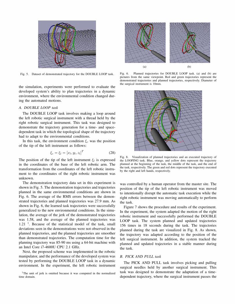
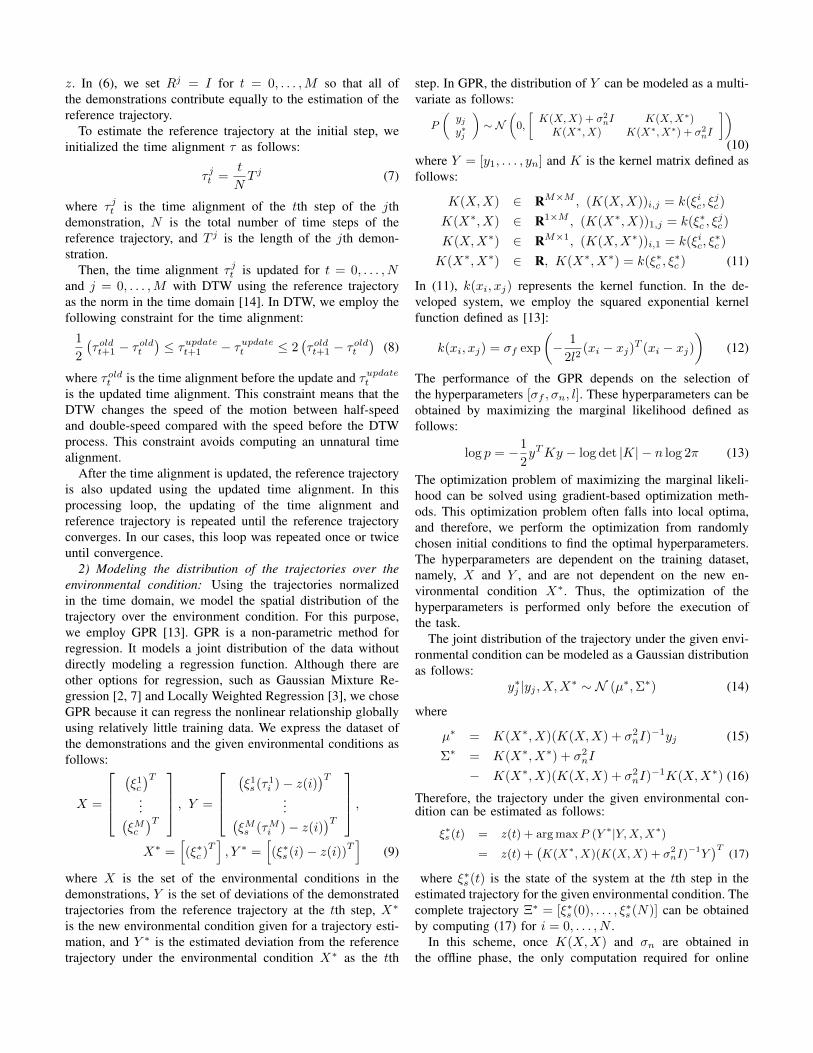
Fig. 5. Dataset of demonstrated trajectory for the DOUBLE LOOP task.

the simulation, experiments were performed to evaluate thedeveloped system’s ability to plan trajectories in a dynamicenvironment, where the environmental condition changed dur-ing the automated motions.

A. DOUBLE LOOP task

The DOUBLE LOOP task involves making a loop aroundthe left robotic surgical instrument with a thread held by theright robotic surgical instrument. This task was designed todemonstrate the trajectory generation for a time- and space-dependent task in which the topological shape of the trajectoryhad to adapt to the environmental conditions.

In this task, the environment condition ξc was the positionof the tip of the left instrument as follows:

ξc = ξl = [xl, yl, zl]T (28)

The position of the tip of the left instrument ξl is expressedin the coordinates of the base of the left robotic arm. Thetransformation from the coordinates of the left robotic instru-ment to the coordinates of the right robotic instrument wasunknown.

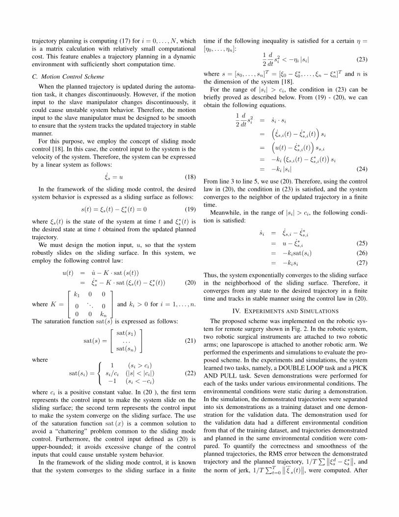
The demonstration trajectory data set in this experiment isshown in Fig. 5. The demonstration trajectories and trajectoriesplanned in the same environmental conditions are shown inFig. 6. The average of the RMS errors between the demon-strated trajectories and planned trajectories was 27.9 mm. Asshown in Fig. 6, the learned task trajectories were successfullygeneralized to the new environmental conditions. In the simu-lation, the average of the jerk of the demonstrated trajectorieswas 1.58, and the average of the planned trajectories was1.21 1. Because of the statistical model of the task, smalldeviations seen in the demonstrations were not observed in theplanned trajectories, and the planned trajectories are smootherthan demonstrated trajectories. The computation time for theplanning trajectory was 85-90 ms using a 64-bit machine withan Intel Core i7-4600U CPU 2.1 GHz.

Next, the proposed scheme was implemented in the roboticmanipulator, and the performance of the developed system wastested by performing the DOUBLE LOOP task in a dynamicenvironment. In the experiment, the left robotic instrument

1The unit of jerk is omitted because it was computed in the normalizedtime domain.

(a) (b)

Fig. 6. Planned trajectories for DOUBLE LOOP task. (a) and (b) arepictures from the same viewpoint. Red and green trajectories represent thedemonstrated trajectories and planned trajectories, respectively. Diameter ofthe surgical instrument is 10mm.

Fig. 8. Visualization of planned trajectories and an executed trajectory ofthe LOOPING task. Blue, orange, and yellow dots represent the trajectoryplanned at the beginning of the task, the middle of the task, and the end ofthe task, respectively. The green and red dots represent the trajectory executedby the right and left hands, respectively.

was controlled by a human operator from the master site. Theposition of the tip of the left robotic instrument was movedto intentionally disrupt the automatic task execution while theright robotic instrument was moving automatically to performthe task.

Figure 7 shows the procedure and results of the experiment.In the experiment, the system adapted the motion of the rightrobotic instrument and successfully performed the DOUBLELOOP task. The system planned and updated trajectories156 times in 18 seconds during the task. The trajectoriesplanned during the task are visualized in Fig. 8. As shown,the trajectory was adapted according to the position of theleft surgical instrument. In addition, the system tracked theplanned and updated trajectories in a stable manner duringthe task.

B. PICK AND PULL task

The PICK AND PULL task involves picking and pullingsurgical needles held by another surgical instrument. Thistask was designed to demonstrate the adaptation of a time-dependent trajectory, where the surgical instrument passes the

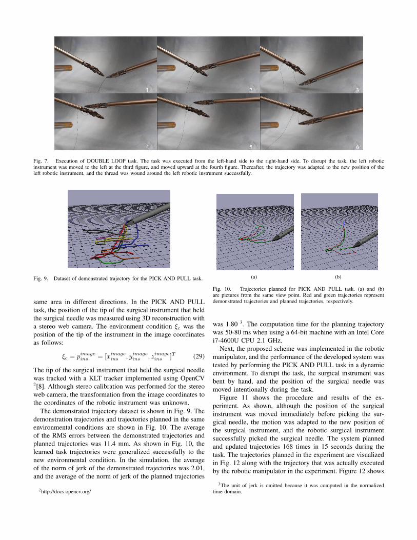
Fig. 7. Execution of DOUBLE LOOP task. The task was executed from the left-hand side to the right-hand side. To disrupt the task, the left roboticinstrument was moved to the left at the third figure, and moved upward at the fourth figure. Thereafter, the trajectory was adapted to the new position of theleft robotic instrument, and the thread was wound around the left robotic instrument successfully.

Fig. 9. Dataset of demonstrated trajectory for the PICK AND PULL task.

same area in different directions. In the PICK AND PULLtask, the position of the tip of the surgical instrument that heldthe surgical needle was measured using 3D reconstruction witha stereo web camera. The environment condition ξc was theposition of the tip of the instrument in the image coordinatesas follows:

ξc = pimageins = [ximage

ins , yimageins , zimage

ins ]T (29)

The tip of the surgical instrument that held the surgical needlewas tracked with a KLT tracker implemented using OpenCV2[8]. Although stereo calibration was performed for the stereoweb camera, the transformation from the image coordinates tothe coordinates of the robotic instrument was unknown.

The demonstrated trajectory dataset is shown in Fig. 9. Thedemonstration trajectories and trajectories planned in the sameenvironmental conditions are shown in Fig. 10. The averageof the RMS errors between the demonstrated trajectories andplanned trajectories was 11.4 mm. As shown in Fig. 10, thelearned task trajectories were generalized successfully to thenew environmental condition. In the simulation, the averageof the norm of jerk of the demonstrated trajectories was 2.01,and the average of the norm of jerk of the planned trajectories

2http://docs.opencv.org/

(a) (b)

Fig. 10. Trajectories planned for PICK AND PULL task. (a) and (b)are pictures from the same view point. Red and green trajectories representdemonstrated trajectories and planned trajectories, respectively.

was 1.80 3. The computation time for the planning trajectorywas 50-80 ms when using a 64-bit machine with an Intel Corei7-4600U CPU 2.1 GHz.

Next, the proposed scheme was implemented in the roboticmanipulator, and the performance of the developed system wastested by performing the PICK AND PULL task in a dynamicenvironment. To disrupt the task, the surgical instrument wasbent by hand, and the position of the surgical needle wasmoved intentionally during the task.

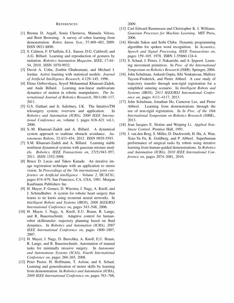
Figure 11 shows the procedure and results of the ex-periment. As shown, although the position of the surgicalinstrument was moved immediately before picking the sur-gical needle, the motion was adapted to the new position ofthe surgical instrument, and the robotic surgical instrumentsuccessfully picked the surgical needle. The system plannedand updated trajectories 168 times in 15 seconds during thetask. The trajectories planned in the experiment are visualizedin Fig. 12 along with the trajectory that was actually executedby the robotic manipulator in the experiment. Figure 12 shows

3The unit of jerk is omitted because it was computed in the normalizedtime domain.

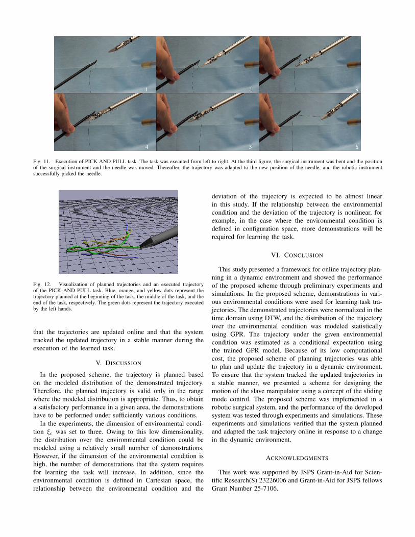
Fig. 11. Execution of PICK AND PULL task. The task was executed from left to right. At the third figure, the surgical instrument was bent and the positionof the surgical instrument and the needle was moved. Thereafter, the trajectory was adapted to the new position of the needle, and the robotic instrumentsuccessfully picked the needle.

Fig. 12. Visualization of planned trajectories and an executed trajectoryof the PICK AND PULL task. Blue, orange, and yellow dots represent thetrajectory planned at the beginning of the task, the middle of the task, and theend of the task, respectively. The green dots represent the trajectory executedby the left hands.

that the trajectories are updated online and that the systemtracked the updated trajectory in a stable manner during theexecution of the learned task.

V. DISCUSSION

In the proposed scheme, the trajectory is planned basedon the modeled distribution of the demonstrated trajectory.Therefore, the planned trajectory is valid only in the rangewhere the modeled distribution is appropriate. Thus, to obtaina satisfactory performance in a given area, the demonstrationshave to be performed under sufficiently various conditions.

In the experiments, the dimension of environmental condi-tion ξc was set to three. Owing to this low dimensionality,the distribution over the environmental condition could bemodeled using a relatively small number of demonstrations.However, if the dimension of the environmental condition ishigh, the number of demonstrations that the system requiresfor learning the task will increase. In addition, since theenvironmental condition is defined in Cartesian space, therelationship between the environmental condition and the

deviation of the trajectory is expected to be almost linearin this study. If the relationship between the environmentalcondition and the deviation of the trajectory is nonlinear, forexample, in the case where the environmental condition isdefined in configuration space, more demonstrations will berequired for learning the task.

VI. CONCLUSION

This study presented a framework for online trajectory plan-ning in a dynamic environment and showed the performanceof the proposed scheme through preliminary experiments andsimulations. In the proposed scheme, demonstrations in vari-ous environmental conditions were used for learning task tra-jectories. The demonstrated trajectories were normalized in thetime domain using DTW, and the distribution of the trajectoryover the environmental condition was modeled statisticallyusing GPR. The trajectory under the given environmentalcondition was estimated as a conditional expectation usingthe trained GPR model. Because of its low computationalcost, the proposed scheme of planning trajectories was ableto plan and update the trajectory in a dynamic environment.To ensure that the system tracked the updated trajectories ina stable manner, we presented a scheme for designing themotion of the slave manipulator using a concept of the slidingmode control. The proposed scheme was implemented in arobotic surgical system, and the performance of the developedsystem was tested through experiments and simulations. Theseexperiments and simulations verified that the system plannedand adapted the task trajectory online in response to a changein the dynamic environment.

ACKNOWLEDGMENTS

This work was supported by JSPS Grant-in-Aid for Scien-tific Research(S) 23226006 and Grant-in-Aid for JSPS fellowsGrant Number 25-7106.

REFERENCES

[1] Brenna D. Argall, Sonia Chernova, Manuela Veloso,and Brett Browning. A survey of robot learning fromdemonstration. Robot. Auton. Syst., 57:469–483, 2009.ISSN 0921-8890.

[2] S. Calinon, F. D’halluin, E.L. Sauser, D.G. Caldwell, andA.G. Billard. Learning and reproduction of gestures byimitation. Robotics Automation Magazine, IEEE, 17:44–54, 2010. ISSN 1070-9932.

[3] David A. Cohn, Zoubin Ghahramani, and Michael I.Jordan. Active learning with statistical models. Journalof Artificial Intelligence Research, 4:129–145, 1996.

[4] Elena Gribovskaya, Seyed Mohammad Khansari-Zadeh,and Aude Billard. Learning non-linear multivariatedynamics of motion in robotic manipulators. The In-ternational Journal of Robotics Research, 30(1):80–117,2011.

[5] G.S. Guthart and Jr. Salisbury, J.K. The IntuitiveTMtelesurgery system: overview and application. InRobotics and Automation (ICRA), 2000 IEEE Interna-tional Conference on, volume 1, pages 618–621 vol.1,2000.

[6] S.-M. Khansari-Zadeh and A. Billard. A dynamicalsystem approach to realtime obstacle avoidance. Au-tonomous Robots, 32:433–454, 2012. ISSN 0929-5593.

[7] S.M. Khansari-Zadeh and A. Billard. Learning stablenonlinear dynamical systems with gaussian mixture mod-els. Robotics, IEEE Transactions on, 27(5):943–957,2011. ISSN 1552-3098.

[8] Bruce D. Lucas and Takeo Kanade. An iterative im-age registration technique with an application to stereovision. In Proceedings of the 7th international joint con-ference on Artificial intelligence - Volume 2, IJCAI’81,pages 674–679, San Francisco, CA, USA, 1981. MorganKaufmann Publishers Inc.

[9] H. Mayer, F. Gomez, D. Wierstra, I. Nagy, A. Knoll, andJ. Schmidhuber. A system for robotic heart surgery thatlearns to tie knots using recurrent neural networks. InIntelligent Robots and Systems (IROS), 2006 IEEE/RSJInternational Conference on, pages 543–548, 2006.

[10] H. Mayer, I. Nagy, A. Knoll, E.U. Braun, R. Lange,and R. Bauernschmitt. Adaptive control for human-robot skilltransfer: trajectory planning based on fluiddynamics. In Robotics and Automation (ICRA), 2007IEEE International Conference on, pages 1800–1807,2007.

[11] H. Mayer, I. Nagy, D. Burschka, A. Knoll, E.U. Braun,R. Lange, and R. Bauernschmitt. Automation of manualtasks for minimally invasive surgery. In Autonomicand Autonomous Systems (ICAS), Fourth InternationalConference on, pages 260–265, 2008.

[12] Peter Pastor, H. Hoffmann, T. Asfour, and S. Schaal.Learning and generalization of motor skills by learningfrom demonstration. In Robotics and Automation (ICRA),2009 IEEE International Conference on, pages 763–768,

2009.[13] Carl Edward Rasmussen and Christopher K. I. Williams.

Gaussian Processes for Machine Learning. MIT Press,2006.

[14] Hiroaki Sakoe and Seibi Chiba. Dynamic programmingalgorithm for spoken word recognition. In Acoustics,Speech and Signal Processing, IEEE Transactions on,pages 159–165. 1978. ISBN 1-55860-124-4.

[15] S. Schaal, J. Peters, J. Nakanishi, and A. Ijspeert. Learn-ing movement primitives. In Proc. of the InternationalSymposium on Robotics Research (ISRR). Springer, 2004.

[16] John Schulman, Ankush Gupta, Sibi Venkatesan, MalloryTayson-Frederick, and Pieter Abbeel. A case study oftrajectory transfer through non-rigid registration for asimplified suturing scenario. In Intelligent Robots andSystems (IROS), 2013 IEEE/RSJ International Confer-ence on, pages 4111–4117, 2013.

[17] John Schulman, Jonathan Ho, Cameron Lee, and PieterAbbeel. Learning from demonstrations through theuse of non-rigid registration. In In Proc. of the 16thInternational Symposium on Robotics Research (ISRR).,2013.

[18] Jean Jacques E. Slotine and Weiping Li. Applied Non-linear Control. Prentice Hall, 1991.

[19] J. van den Berg, S. Miller, D. Duckworth, H. Hu, A. Wan,Xiao-Yu Fu, K. Goldberg, and P. Abbeel. Superhumanperformance of surgical tasks by robots using iterativelearning from human-guided demonstrations. In Roboticsand Automation (ICRA), 2010 IEEE International Con-ference on, pages 2074–2081, 2010.