Online predictionwith expert advise

Jyrki Kivinen

Australian National University

http://axiom.anu.edu.au/~kivinen

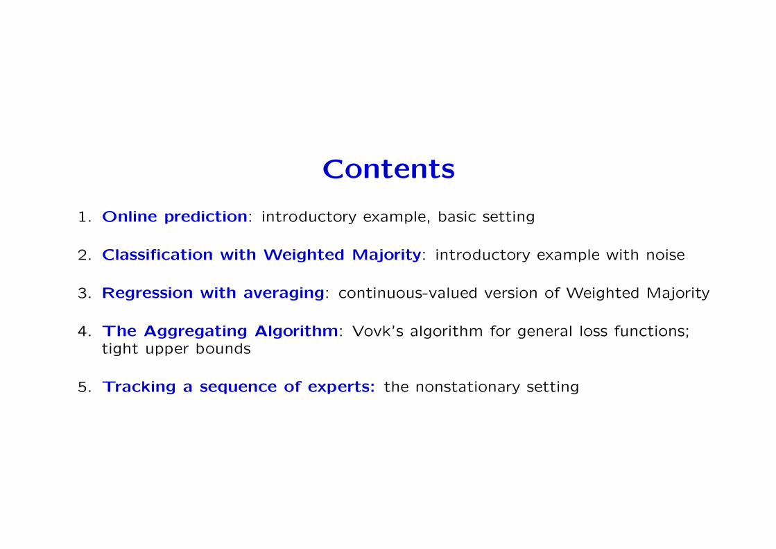
Contents

1. Online prediction: introductory example, basic setting

2. Classification with Weighted Majority: introductory example with noise

3. Regression with averaging: continuous-valued version of Weighted Majority

4. The Aggregating Algorithm: Vovk’s algorithm for general loss functions;tight upper bounds

5. Tracking a sequence of experts: the nonstationary setting

Introductory example

• Each morning you must predict whether it will rain or not.

• At the end of the day we observe whether rain actually did occur.

• If your prediction was incorrect, you incur one unit of loss.

• Repeat this for T days (say T = 365); try to minimise your total loss.

• You do not know anything about meteorology, but have lots of other sources,called experts, to help you.

• The experts are given to you, you are not responsible for training them etc.

• You expect to do well if at least some experts are good.

Let there be n experts denoted by Ei, i = 1, . . . , n (say n = 1000).

• Experts may or may not have hidden side information.

• Experts may or may not have dependencies between each other.

Example:

E1: Canberra Times weather columnE2: New York Times weather columnE3: Australian Bureau of Meteorology web site. . .Ei: your own backprop net with 10 hidden nodesEi+1: your own backprop net with 100 hidden nodesEi+2: it rains if you washed your car yesterday. . .En−3: it rains if it rained yesterdayEn−2: it never rainsEn−1: it always rainsEn: toss a coin

(Almost) realistic examples

Modifications of the basic online expert prediction algorithm have been successfulon these problems on realistic simulation data.

Problem: Stock portfolio managementExperts: “Invest all your money in stock s”

Problem: Equalisation (in signal processing)Experts: Copies of LMS with different learning rates

Problem: Disk spin-down on laptopExperts: “Spin down after s seconds of idle time”

Problem: Disk cachingExperts: RAND, FIFO, LIFO, LRU, MRU, . . .

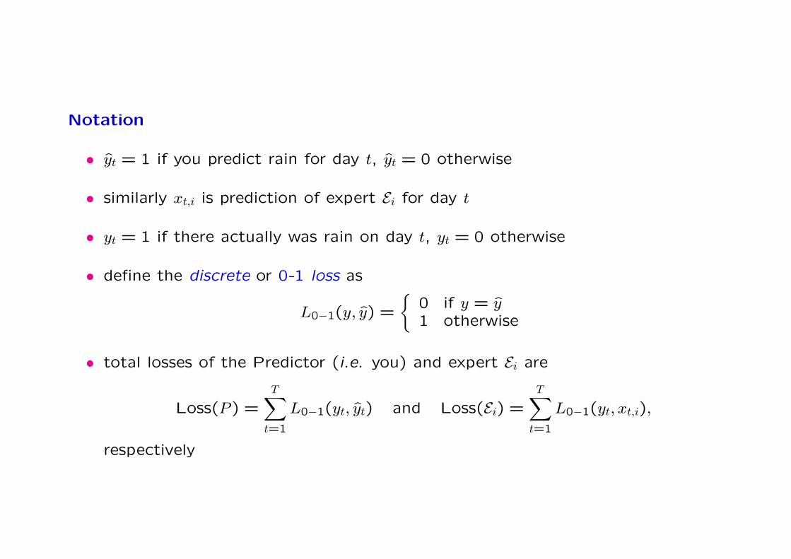
Notation

• yt = 1 if you predict rain for day t, yt = 0 otherwise

• similarly xt,i is prediction of expert Ei for day t

• yt = 1 if there actually was rain on day t, yt = 0 otherwise

• define the discrete or 0-1 loss as

L0−1(y, y) =

0 if y = y1 otherwise

• total losses of the Predictor (i.e. you) and expert Ei are

Loss(P ) =T∑

t=1

L0−1(yt, yt) and Loss(Ei) =T∑

t=1

L0−1(yt, xt,i),

respectively

Basic setting

The following is repeated at each day t:

1. You see the experts’ predictions xt,i, i = 1, . . . , n.

2. You make your prediction yt.

3. You see the actual outcome yt.

When you make your prediction for day t, you remember what happened at days1, . . . , n− 1. In particular, you know the experts’ past performances.

• Want to achieve small total loss for the predictor assuming at least oneexpert has small total loss.

• Start with the simplistic case where one expert has loss zero (but of coursewe do not in advance know which).

Algorithm (Weighted Majority for noise-free case)

(We say “noise-free” to denote that at least one expert is perfectly correct for thewhole sequence.)

• Say that expert Ei is consistent up to time t if xτ,i = yτ for τ = 1, . . . , t− 1.

• At time t, predict according to the majority of experts consistent up to thattime. (Break ties arbitrarily.)

We are assuming that at least one expert is consistent for the whole sequence sothis is well defined.

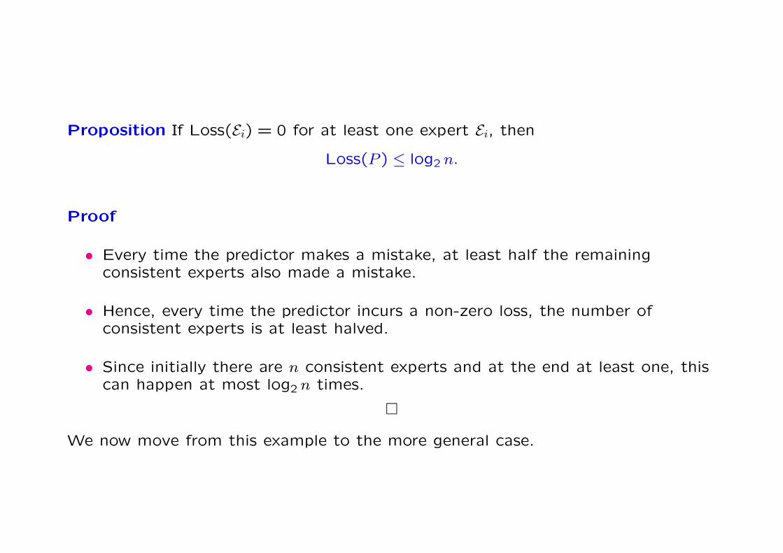
Proposition If Loss(Ei) = 0 for at least one expert Ei, then

Loss(P ) ≤ log2 n.

Proof

• Every time the predictor makes a mistake, at least half the remainingconsistent experts also made a mistake.

• Hence, every time the predictor incurs a non-zero loss, the number ofconsistent experts is at least halved.

• Since initially there are n consistent experts and at the end at least one, thiscan happen at most log2 n times.

We now move from this example to the more general case.

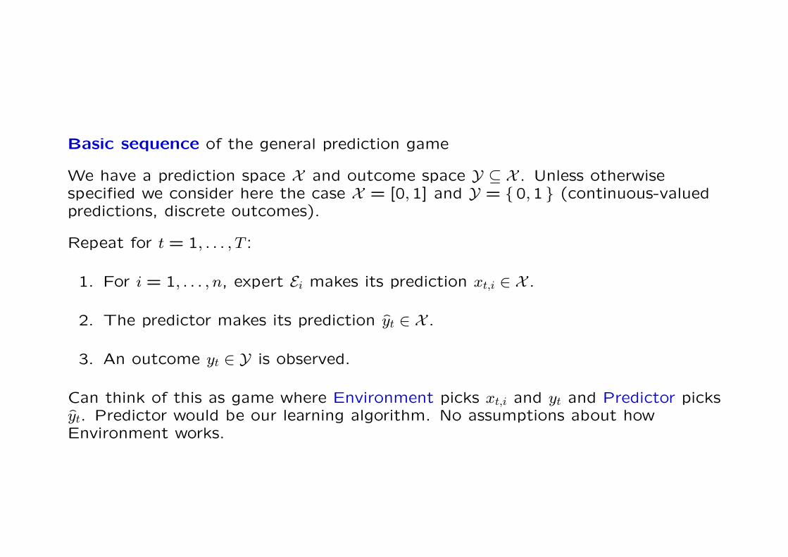
Basic sequence of the general prediction game

We have a prediction space X and outcome space Y ⊆ X . Unless otherwisespecified we consider here the case X = [0,1] and Y = 0,1 (continuous-valuedpredictions, discrete outcomes).

Repeat for t = 1, . . . , T :

1. For i = 1, . . . , n, expert Ei makes its prediction xt,i ∈ X .

2. The predictor makes its prediction yt ∈ X .

3. An outcome yt ∈ Y is observed.

Can think of this as game where Environment picks xt,i and yt and Predictor picksyt. Predictor would be our learning algorithm. No assumptions about howEnvironment works.

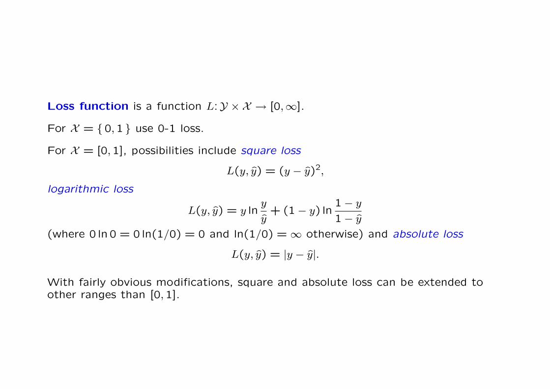
Loss function is a function L:Y × X → [0,∞].

For X = 0,1 use 0-1 loss.

For X = [0,1], possibilities include square loss

L(y, y) = (y − y)2,

logarithmic loss

L(y, y) = y lny

y+ (1− y) ln

1− y

1− y

(where 0 ln 0 = 0 ln(1/0) = 0 and ln(1/0) = ∞ otherwise) and absolute loss

L(y, y) = |y − y|.

With fairly obvious modifications, square and absolute loss can be extended toother ranges than [0,1].

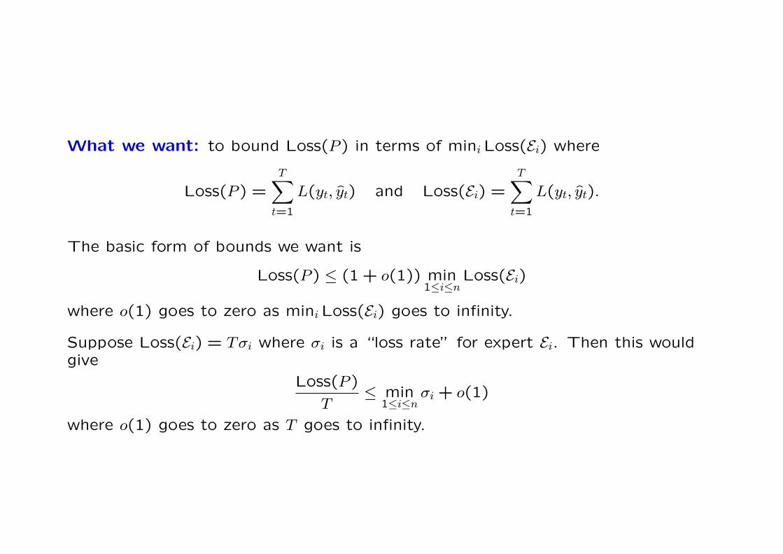
What we want: to bound Loss(P ) in terms of mini Loss(Ei) where

Loss(P ) =T∑

t=1

L(yt, yt) and Loss(Ei) =T∑

t=1

L(yt, yt).

The basic form of bounds we want is

Loss(P ) ≤ (1 + o(1)) min1≤i≤n

Loss(Ei)

where o(1) goes to zero as mini Loss(Ei) goes to infinity.

Suppose Loss(Ei) = Tσi where σi is a “loss rate” for expert Ei. Then this wouldgive

Loss(P )

T≤ min

1≤i≤nσi + o(1)

where o(1) goes to zero as T goes to infinity.

What our algorithm(s) will achieve (brief preview)

For square loss, log loss etc. we can guarantee

Loss(P ) ≤ min1≤i≤n

Loss(Ei) + c lnn.

For absolute loss can guarantee for any 0 < ε < 1 (given a priori) that

Loss(P ) ≤ (1 + ε) min1≤i≤n

Loss(Ei) +c

εlnn.

For discrete predictions can only guarantee

Loss(P ) ≤ (2 + ε) min1≤i≤n

Loss(Ei) +c

εlnn.

Here c > 0 is a constant that depends only on the loss function.

The trade-off parameter ε is determined by the learning rate of the algorithmwhich (in the basic version of the algorithm) must be fixed in advance.

Plug in Loss(Ei) = Tσi.

For square loss etc. we get

Loss(P )

T≤ min

1≤i≤nσi +

c lnn

T.

For absolute loss, by choosing ε =√

C lnn/(mini Loss(Ei)) and using σi ≤ 1 we get

Loss(P )

T≤ min

1≤i≤nσi + 2

√c lnn

T+ O

(1

T

).

In these cases, the loss rate of predictor converges to that of the best expert.(The choice of ε is an issue though.)

Important: The dependence on n is always only logarithmic.

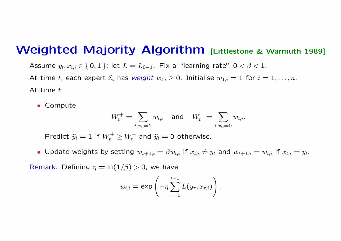
Weighted Majority Algorithm [Littlestone & Warmuth 1989]

Assume yt, xt,i ∈ 0,1 ; let L = L0−1. Fix a “learning rate” 0 < β < 1.

At time t, each expert Ei has weight wt,i ≥ 0. Initialise w1,i = 1 for i = 1, . . . , n.

At time t:

• Compute

W+t =

∑i:xt,i=1

wt,i and W−t =

∑i:xt,i=0

wt,i.

Predict yt = 1 if W+t ≥ W−

t and yt = 0 otherwise.

• Update weights by setting wt+1,i = βwt,i if xt,i 6= yt and wt+1,i = wt,i if xt,i = yt.

Remark: Defining η = ln(1/β) > 0, we have

wt,i = exp

(−η

t−1∑τ=1

L(yτ , xτ,i)

).

Write Wt = W+t + W−

t =∑n

i=1 wt,i.

Lemma For c = 1/ ln(2/(1 + β)) we have

L(yt, yt) ≤ −c lnWt+1

Wt.

Proof Clear if L(yt, yt) = 0 since c > 0 and Wt+1 ≤ Wt.

Consider the case L(yt, yt) = 1, say yt = 1 and yt = 0. Then W+t ≤ Wt/2. We have

Wt+1 = W+t + βW−

t

= (1− β)W+t + β(W+

t + W−t )

≤ (1− β)Wt

2+ βWt

from which c ln(Wt/Wt+1) ≥ 1 follows.

Theorem For any expert Ei we have

Loss(P ) ≤ cηLoss(Ei) + c lnn

where

c =

(ln

2

1 + β

)−1

and η = ln1

β.

Proof: Pick any expert Ei. From Claim 1 we have

Loss(P ) ≤ −c

T∑t=1

(lnWt+1 − lnWt)

= −c lnWT+1 + c lnW1

≤ −c lnwt+1,i + c lnW1

= cη

T∑t=1

L(yt, xt,i) + c lnn.

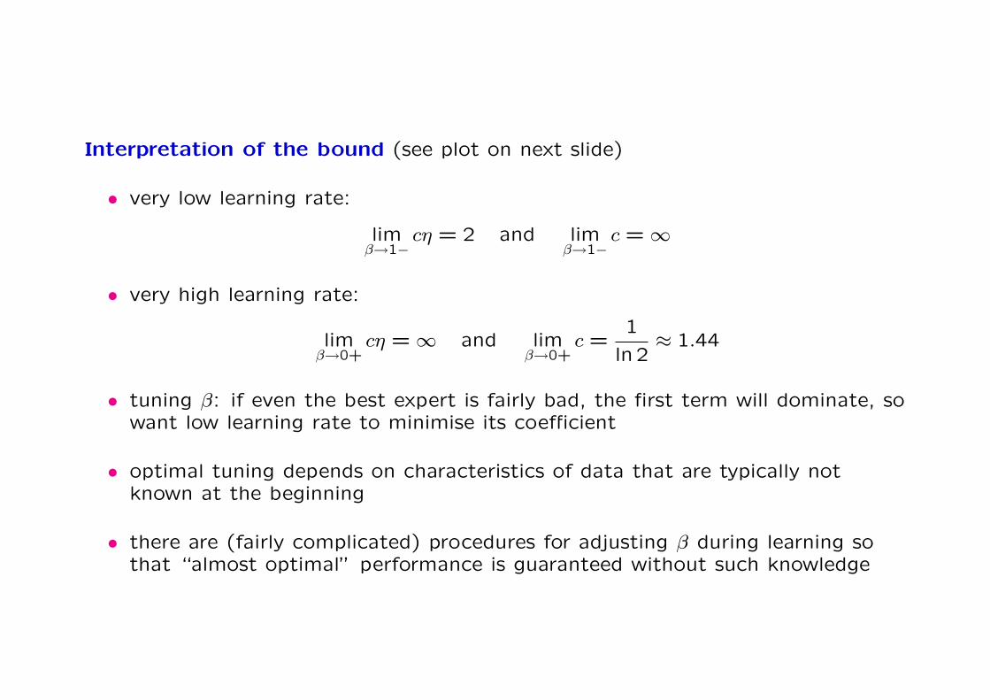
Interpretation of the bound (see plot on next slide)

• very low learning rate:

limβ→1−

cη = 2 and limβ→1−

c = ∞

• very high learning rate:

limβ→0+

cη = ∞ and limβ→0+

c =1

ln2≈ 1.44

• tuning β: if even the best expert is fairly bad, the first term will dominate, sowant low learning rate to minimise its coefficient

• optimal tuning depends on characteristics of data that are typically notknown at the beginning

• there are (fairly complicated) procedures for adjusting β during learning sothat “almost optimal” performance is guaranteed without such knowledge

The curve of points (x, y) = (cη, c) for β ∈ (0,1). The asymptotes are x = 2 andy = 1/ ln 2.

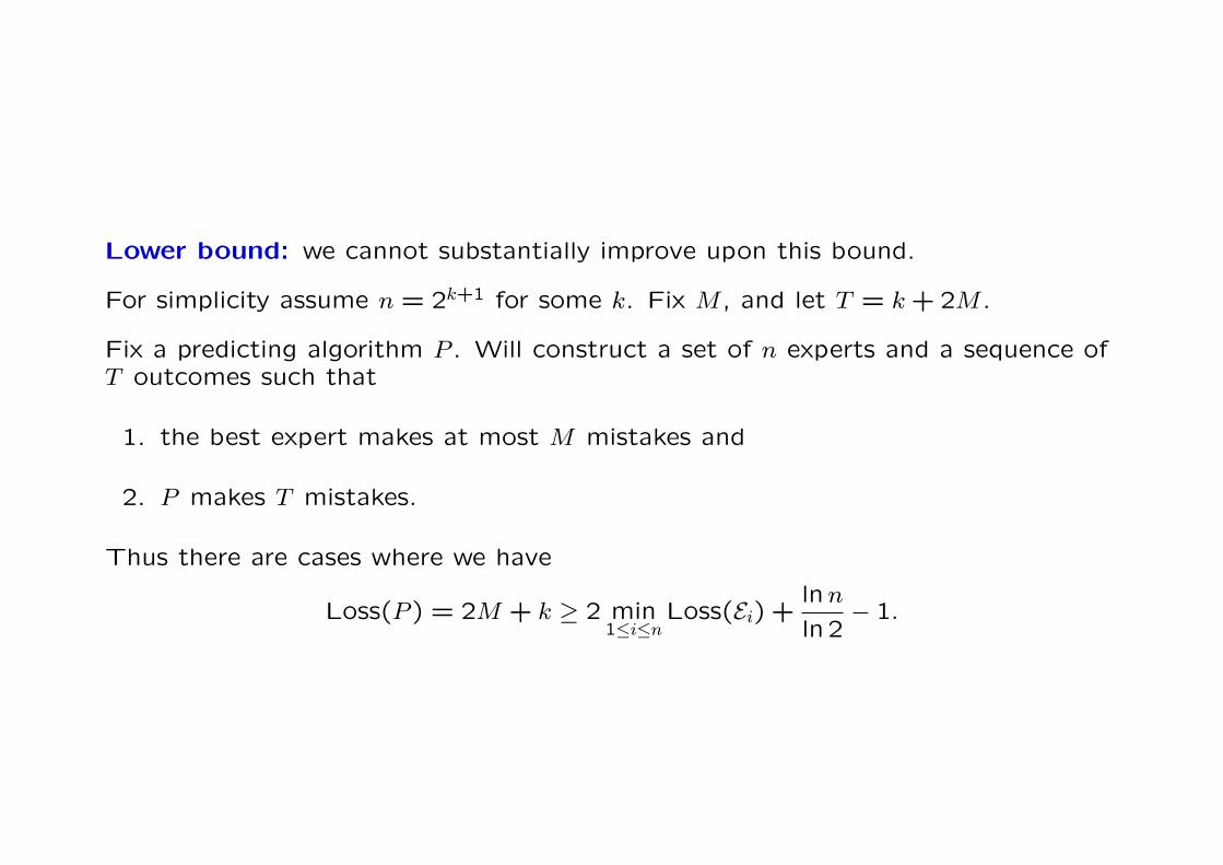
Lower bound: we cannot substantially improve upon this bound.

For simplicity assume n = 2k+1 for some k. Fix M , and let T = k + 2M .

Fix a predicting algorithm P . Will construct a set of n experts and a sequence ofT outcomes such that

1. the best expert makes at most M mistakes and

2. P makes T mistakes.

Thus there are cases where we have

Loss(P ) = 2M + k ≥ 2 min1≤i≤n

Loss(Ei) +lnn

ln 2− 1.

Lower bound construction For i = 1, . . . ,2k, define experts Ei and Ei+2k asfollows:

• For t = 1, . . . , k, both Ei and Ei+2k predict 1 if the binary representation of(i− 1) has 1 in position t.

• For t = k + 1, . . . , k + 2M , Ei always predicts 1 and Ei+2k always predicts 0.

After first k time steps there is exactly one i such that neither Ei nor Ei+2k hasmade any mistakes yet.

During the remaining time steps either Ei or Ei+2k must be right at least half thetime.

Thus for any sequence of outcomes there is an expert with at most M mistakes.We simply choose the outcomes to be opposite to whatever P predicts.

Example k = 2, n = 2k+1 = 8, M = 3; T = k + 2M = 8.

The experts’ predictions are as follows:

t 1 2 3 4 5 6 7 8E1 0 0 1 1 1 1 1 1E2 1 0 1 1 1 1 1 1E3 0 1 1 1 1 1 1 1E4 1 1 1 1 1 1 1 1E5 0 0 0 0 0 0 0 0E6 1 0 0 0 0 0 0 0E7 0 1 0 0 0 0 0 0E8 1 1 0 0 0 0 0 0

Suppose the outcome sequence is

(y1, . . . , y8) = (1,0,1,0,0,0,0,1).

After k = 2 steps E2 and E6 have loss 0.

After the whole sequence, E6 has loss 2 ≤ M (and E2 has loss 4 = 2M − 2).

Weighted Average AlgorithmAssume 0 ≤ xt,i ≤ 1 and yt ∈ 0,1 . Fix a learning rate η > 0.

At time t, each expert Ei has weight wt,i ≥ 0. Initialise w1,i = 1 for i = 1, . . . , n.

At time t:

• For i = 1, . . . , n let vt,i = wt,i/Wt where Wt =∑n

i=1 wt,i. Predict with

yt = vt · xt =n∑

i=1

vt,ixt,i.

• Update weights by setting

wt+1,i = wt,i exp(−ηL(yt, xt,i)).

Remark: As with Weighted Majority we have

wt,i = w1,i exp

(−η

t−1∑τ=1

L(yτ , xτ,i)

).

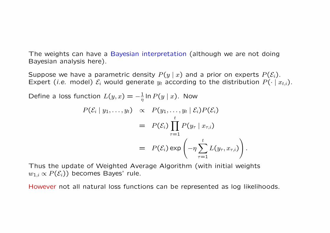
The weights can have a Bayesian interpretation (although we are not doingBayesian analysis here).

Suppose we have a parametric density P (y | x) and a prior on experts P (Ei).Expert (i.e. model) Ei would generate yt according to the distribution P (· | xt,i).

Define a loss function L(y, x) = −1ηlnP (y | x). Now

P (Ei | y1, . . . , yt) ∝ P (y1, . . . , yt | Ei)P (Ei)

= P (Ei)t∏

τ=1

P (yτ | xτ,i)

= P (Ei) exp

(−η

t∑τ=1

L(yτ , xτ,i)

).

Thus the update of Weighted Average Algorithm (with initial weightsw1,i ∝ P (Ei)) becomes Bayes’ rule.

However not all natural loss functions can be represented as log likelihoods.

Analysis of the algorithm goes, at high level, as follows.

1. Find η > 0 and c > 0 such that we can guarantee

L(yt, yt) ≤ −c lnWt+1

Wt.

2. Sum over t = 1, . . . , T .

Step 2 is easy and independent of the loss function; we essentially already did it inthe analysis of Weighted Majority.

Step 1 is technical and uses properties of the actual loss function. Howevergeneral results exist that handle large classes of loss functions. The case c = 1/ηis of special interest.

Remark: In Step 2 we do not need the assumption yt = vt · xt. In many casesStep 1 can actually be performed with better constants using some otherprediction. This leads to Vovk’s Aggregating Algorithm.

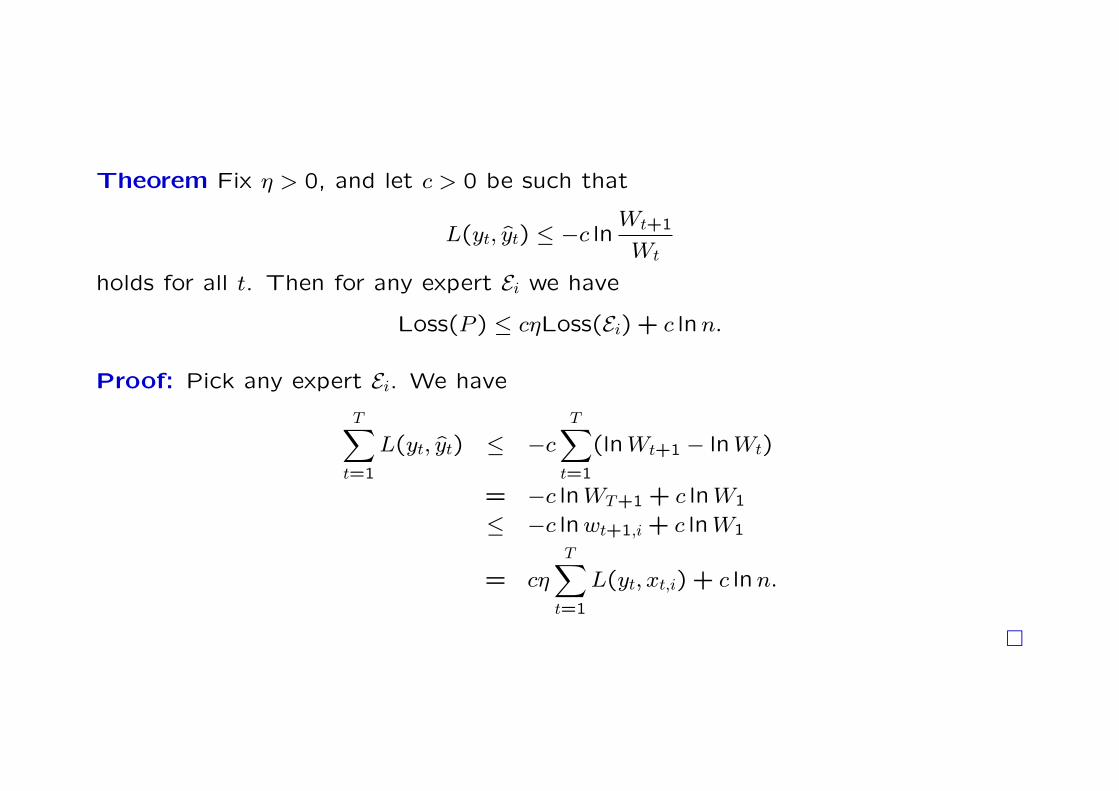
Theorem Fix η > 0, and let c > 0 be such that

L(yt, yt) ≤ −c lnWt+1

Wt

holds for all t. Then for any expert Ei we have

Loss(P ) ≤ cηLoss(Ei) + c lnn.

Proof: Pick any expert Ei. We have

T∑t=1

L(yt, yt) ≤ −c

T∑t=1

(lnWt+1 − lnWt)

= −c lnWT+1 + c lnW1

≤ −c lnwt+1,i + c lnW1

= cη

T∑t=1

L(yt, xt,i) + c lnn.

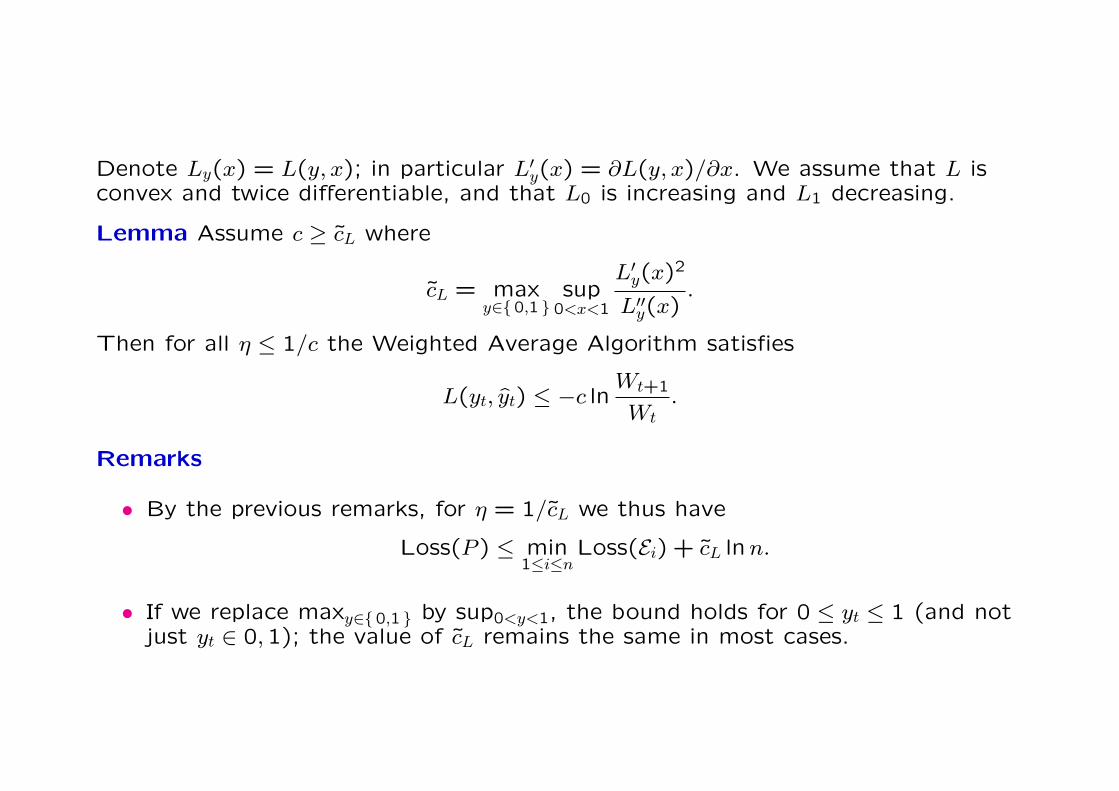
Denote Ly(x) = L(y, x); in particular L′y(x) = ∂L(y, x)/∂x. We assume that L isconvex and twice differentiable, and that L0 is increasing and L1 decreasing.

Lemma Assume c ≥ cL where

cL = maxy∈0,1

sup0<x<1

L′y(x)2

L′′y(x).

Then for all η ≤ 1/c the Weighted Average Algorithm satisfies

L(yt, yt) ≤ −c lnWt+1

Wt.

Remarks

• By the previous remarks, for η = 1/cL we thus have

Loss(P ) ≤ min1≤i≤n

Loss(Ei) + cL lnn.

• If we replace maxy∈0,1 by sup0<y<1, the bound holds for 0 ≤ yt ≤ 1 (and notjust yt ∈ 0,1); the value of cL remains the same in most cases.

Examples (The last column gives the optimal constant that can be achieved withthe “real” Aggregating Algorithm; more of this later.)

loss function L(y, x) cL cL

square (y − x)2 2 1/2

logarithmic (1− y) ln((1− y)/(1− x)) + y ln(y/x) 1 1

Hellinger 12

((√1− y −

√1− x

)2+(√

y −√

x)2)

1 2−1/2 ≈ 0.71

absolute |y − x| (∞) (∞)

Remark The constant cL can be shown to be optimal, i.e. for any predictor Pthere are sequences such that

Loss(P ) ≥ min1≤i≤n

Loss(Ei) + cL lnn− o(1).

Proof of Lemma: Without loss of generality take c = 1/η. The claim is

L(yt, vt · xt) ≤ −c ln

∑ti=1 wt,i exp(−L(yt, xt,i)/c)

Wt= −c ln

n∑i=1

vt,i exp(−L(yt, xt,i)/c),

or equivalently

exp(−L(yt, vt · xt)/c) ≥n∑

i=1

vt,i exp(−L(yt, xt,i)/c).

Write this as

f(n∑

i=1

vt,ixt,i) ≥n∑

i=1

vt,if(xt,i)

where f(x) = exp(−L(y, x)/c). The assumption implies that f ′′ is negative so theclaim follows by Jensen’s Inequality.

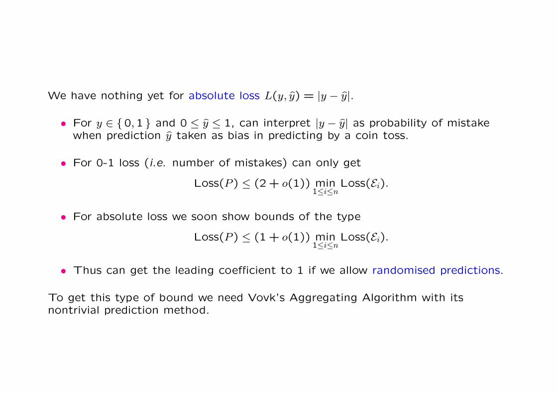
We have nothing yet for absolute loss L(y, y) = |y − y|.

• For y ∈ 0,1 and 0 ≤ y ≤ 1, can interpret |y − y| as probability of mistakewhen prediction y taken as bias in predicting by a coin toss.

• For 0-1 loss (i.e. number of mistakes) can only get

Loss(P ) ≤ (2 + o(1)) min1≤i≤n

Loss(Ei).

• For absolute loss we soon show bounds of the type

Loss(P ) ≤ (1 + o(1)) min1≤i≤n

Loss(Ei).

• Thus can get the leading coefficient to 1 if we allow randomised predictions.

To get this type of bound we need Vovk’s Aggregating Algorithm with itsnontrivial prediction method.

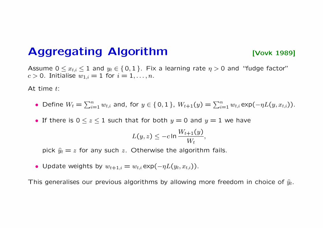
Aggregating Algorithm [Vovk 1989]

Assume 0 ≤ xt,i ≤ 1 and yt ∈ 0,1 . Fix a learning rate η > 0 and “fudge factor”c > 0. Initialise w1,i = 1 for i = 1, . . . , n.

At time t:

• Define Wt =∑n

i=1 wt,i and, for y ∈ 0,1 , Wt+1(y) =∑n

i=1 wt,i exp(−ηL(y, xt,i)).

• If there is 0 ≤ z ≤ 1 such that for both y = 0 and y = 1 we have

L(y, z) ≤ −c lnWt+1(y)

Wt,

pick yt = z for any such z. Otherwise the algorithm fails.

• Update weights by wt+1,i = wt,i exp(−ηL(yt, xt,i)).

This generalises our previous algorithms by allowing more freedom in choice of yt.

• As before we have

wt,i = w1,i exp

(−η

t−1∑τ=1

L(yτ , xτ,i)

).

• Since Wt+1 = Wt+1(yt), it now follows by definition that

L(yt, yt) ≤ −c lnWt+1

Wt.

The problem is choosing (c, η) so that the algorithm never fails.

• If this can be achieved then as before we get

Loss(P ) ≤ cη min1≤i≤n

Loss(Ei) + c lnn.

• Although the prediction rule looks rather abstract as written it usuallybecomes rather simple when c and η are given. Also given η there is a uniquebest value for c, depending only on which loss function we use.

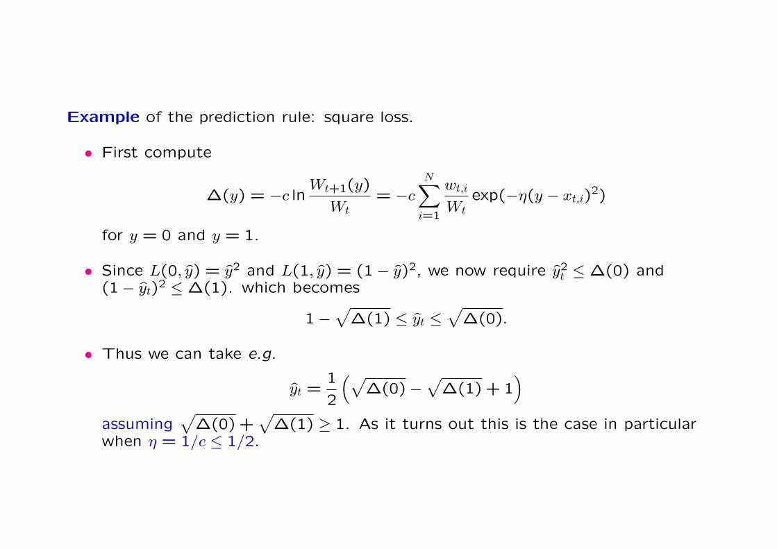
Example of the prediction rule: square loss.

• First compute

∆(y) = −c lnWt+1(y)

Wt= −c

N∑i=1

wt,i

Wtexp(−η(y − xt,i)

2)

for y = 0 and y = 1.

• Since L(0, y) = y2 and L(1, y) = (1− y)2, we now require y2t ≤ ∆(0) and

(1− yt)2 ≤ ∆(1). which becomes

1−√

∆(1) ≤ yt ≤√

∆(0).

• Thus we can take e.g.

yt =1

2

(√∆(0)−

√∆(1) + 1

)assuming

√∆(0) +

√∆(1) ≥ 1. As it turns out this is the case in particular

when η = 1/c ≤ 1/2.

Denote Ly(x) = L(y, x); in particular L′y(x) = ∂L(y, x)/∂x. We assume that L isconvex and twice differentiable, and that L0 is increasing and L1 decreasing.

Lemma Assume c ≥ cL where

cL = sup0<x<1

L′0(x)L′1(x)

2 − L′1(x)L′0(x)

2

L′0(x)L′′1(x)− L′1(x)L

′′0(x)

.

Then the Aggregating Algorithm for any η ≤ 1/c will not fail.

Remarks:

• For examples of cL and respective values of the constant cL for the WeightedAverage Algorithm see the earlier table.

• We get cL ≤ cL directly from the fact that (a + b)/(a′ + b′) ≤ max a/a′, b/b′ for positive a, a′, b, b′.

Absolute loss Pick any η > 0; write β = e−η.

• Can show that the algorithm never fails if c ≥ 1/(2 ln(2/(1 + β))) so

Loss(P ) ≤ln 1

β

2 ln 21+β

min1≤i≤n

Loss(Ei) +1

2 ln 21+β

lnn,

i.e. factor 2 better than Weighed Majority (but this is for a different loss).

• Write σi = Loss(Ei)/T . Optimal choice of β guarantees

Loss(P )

T≤ min

1≤i≤n

(σi +

√σi lnn

T+

lnn

2T ln 2

)but choosing optimal β requires knowing mini Loss(Ei).

• Bounds of the form Loss(P )/T ≤ mini σi + O(T−1/2) can also be achievedwithout additional knowledge by more sophisticated algorithms.

Lower bound for the absolute loss

We show that the square root term is unavoidable. Thus we can only get

Loss(P )

T≤ min

1≤i≤nσi + O(T−1/2)

where again σi is the loss rate for expert Ei. This is weaker than for square loss,log loss etc. which have

Loss(P )

T≤ min

1≤i≤nσi + O(T−1)

The bound is based on a simple probabilistic argument. We show a distributionfor the experts predictions xt,i and outcomes yt such that

E[Loss(P )] ≥ E[ min1≤i≤n

Loss(Ei)] + Ω(√

T )

where E denotes expectation with respect to the choice of xt,i and yt.

Since this holds on average, it of course also holds in worst case.

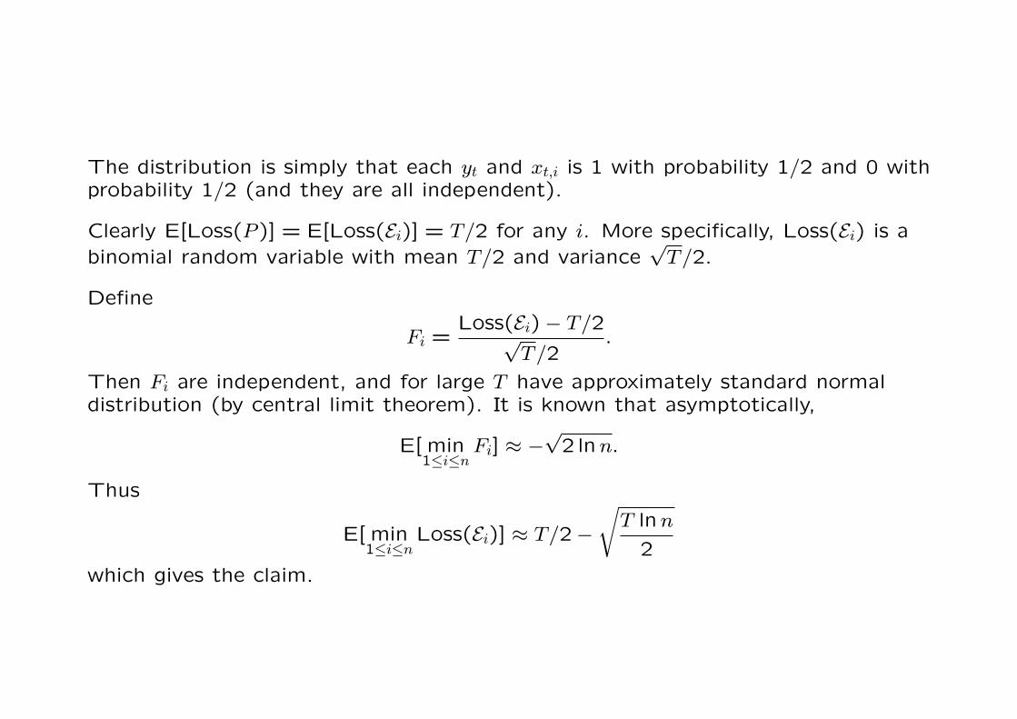
The distribution is simply that each yt and xt,i is 1 with probability 1/2 and 0 withprobability 1/2 (and they are all independent).

Clearly E[Loss(P )] = E[Loss(Ei)] = T/2 for any i. More specifically, Loss(Ei) is abinomial random variable with mean T/2 and variance

√T/2.

Define

Fi =Loss(Ei)− T/2√

T/2.

Then Fi are independent, and for large T have approximately standard normaldistribution (by central limit theorem). It is known that asymptotically,

E[ min1≤i≤n

Fi] ≈ −√

2 lnn.

Thus

E[ min1≤i≤n

Loss(Ei)] ≈ T/2−√

T lnn

2which gives the claim.

Further remarks on the prediction rule

• Weighted average yt = vt · xt will not in general work.

• Special case: for log loss yt = vt · xt is the only thing that works.

• There may not even be any function φ: [0,1] → [0,1] such that yt = φ(vt · xt)would work; however for absolute loss such a function φ does exist.

• The following plot shows the range of legal predictions for absolute loss inthe special case n = 2, (x1, x2) = (1,0).

Upper and lower bounds for prediction y when (x1, x2) = (1,0) as function ofv = w1/(w1 + w2). (Here β = 0.2, i.e. fairly high learning rate.)

Tracking a sequence of experts

Previous methods give good results if a fixed single expert is good over the wholesequence of predictions.

Suppose the process we are predicting is non-stationary. Then perhaps differentexperts are good at different times.

Example Disk caching

• a number of different caching strategies

• some strategies may not be good at all in a given environment

• which one is really the best depends on what activity is going on right now

(There are various other problems in applying prediction algorithms in a cachingsetting.)

Formal setting Consider a sequence of T experts U = (U1, . . . , UT),Ut ∈ Ei | 1 ≤ i ≤ n for all T .

• U has k shifts if there are exactly k indices t ∈ 1, . . . , T − 1 such thatUt 6= Ut+1.

• Expert Ei is active in U if there is at least one index t ∈ 1, . . . , T such thatUt = Ei.

• Let U(k, m) be the set of sequences with k shifts and m active experts, andU(k) = ∪n

m=1U(k, m)

• Define u ∈ [0,1]T by ut = xt,i where i is the index such that Ut = Ei, and let

Loss(U) =T∑

t=1

L(yt, ut).

Assume log loss for now. The basic expert bound

Loss(P ) ≤ min1≤i≤n

Loss(Ei) + lnn

has a (loose) coding theoretic interpretation:

• lnn is the number of bits (using natural logs for convenience) to encode thebest expert

• min1≤i≤n Loss(Ei) is the number of bits to encode the outcomes given thebest expert.

Can we achieve the same here, i.e. have

Loss(P ) ≤ minU∈U(k)

Loss(U) + f(k)

where f(k) is the coding length for a sequence U ∈ U(k)? (And similarly forU(k, m).)

In principle this is possible by considering each U ∈ U(k) as a new expert andrunning Aggregating Algorithm on top of those. However, this would becomputationally prohibitive since we would need |U(k)| weights.

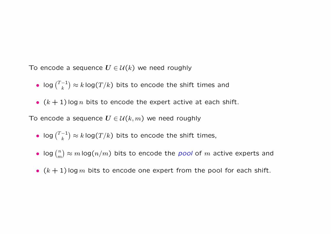
To encode a sequence U ∈ U(k) we need roughly

• log(T−1

k

)≈ k log(T/k) bits to encode the shift times and

• (k + 1) logn bits to encode the expert active at each shift.

To encode a sequence U ∈ U(k, m) we need roughly

• log(T−1

k

)≈ k log(T/k) bits to encode the shift times,

• log(

nm

)≈ m log(n/m) bits to encode the pool of m active experts and

• (k + 1) logm bits to encode one expert from the pool for each shift.

Problem 1: Can we get

Loss(P ) ≤ minU∈U(k)

Loss(U) + O(k logT

k) + O(k logn)

with an efficient algorithm?

Problem 2: Can we get

Loss(P ) ≤ minU∈U(k,m)

Loss(U) + O(k logT

k) + O(m log

n

m) + O(k logm)

with an efficient algorithm?

• Here “efficient” means roughly O(n) time per prediction and update.

• Going from 1 to 2 we replace k logn by k logm + m logn. This is interestingwhen m n and m k.

The basic Aggregating Algorithm will not work here. The exponential updateeradicates the weights of experts that initially perform poorly, and they neverrecover even if they later start performing better.

Thus we need to make sure each expert retains the chance of recovery if itsperformance improves.

Simple method: Divide a fixed portion of the total weight uniformly over all theexperts. Thus everyone has a chance to recover. This is enough to solveProblem 1.

Fancy method(s): Divide a fixed portion of the total weight favouring theexperts that performed well some time in the past. Thus the experts that arein the “pool” have faster recovery. This solves Problem 2.

We next sketch the simple method, called Fixed Share Algorithm.

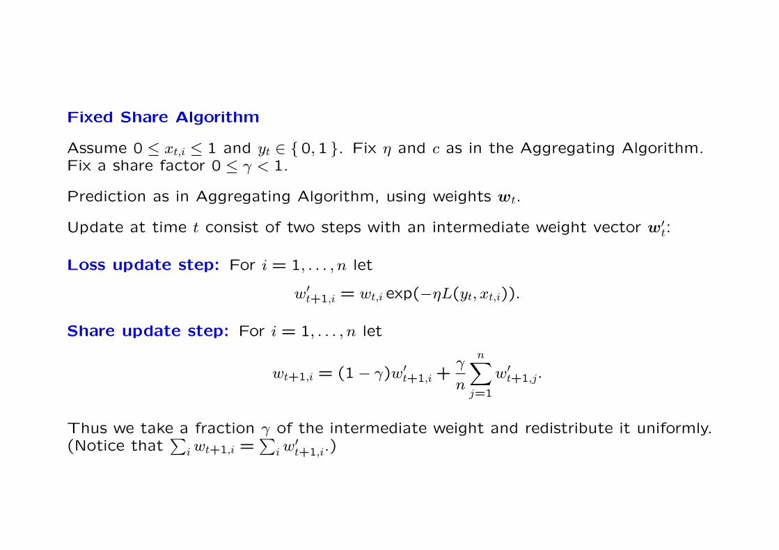
Fixed Share Algorithm

Assume 0 ≤ xt,i ≤ 1 and yt ∈ 0,1 . Fix η and c as in the Aggregating Algorithm.Fix a share factor 0 ≤ γ < 1.

Prediction as in Aggregating Algorithm, using weights wt.

Update at time t consist of two steps with an intermediate weight vector w′t:

Loss update step: For i = 1, . . . , n let

w′t+1,i = wt,i exp(−ηL(yt, xt,i)).

Share update step: For i = 1, . . . , n let

wt+1,i = (1− γ)w′t+1,i +

γ

n

n∑j=1

w′t+1,j.

Thus we take a fraction γ of the intermediate weight and redistribute it uniformly.(Notice that

∑i wt+1,i =

∑i w

′t+1,i.)

For simplicity we state the result only for log loss and omit the finer issues oftuning γ.

Theorem For log loss the Fixed Share Algorithm with

γ =n

n− 1

k

T − 1

satisfies

Loss(P ) ≤ minU∈U(k)

Loss(U) + (k + 1) lnn + k lnT − 1

k+ k.

Thus the bound is as stipulated in Problem 1.

References and further reading

The basic algorithms

Vladimir Vovk: A game of prediction with expert advice. Journal of Computer andSystem Sciences 56:153–173 (1998).

Nick Littlestone and Manfred Warmuth: The weighted majority algorithm. Informationand Computation 108:212–261 (1994).

Dealing with the absolute loss

Nicolo Cesa-Bianchi, Yoav Freund, David Haussler, David Helmbold and RobertSchapire: How to use expert advice. Journal of the ACM 44:427–485 (1997).

Fine-tuning for “nice” loss functions

Jyrki Kivinen, David Haussler and Manfred Warmuth: Sequential prediction of individualsequences under general loss functions. IEEE Transactions on Information Theory44:1906–1925 (1998).

Jyrki Kivinen and Manfred Warmuth: Averaging expert predictions. In EuroCOLT ’99,pp. 153–167 (1999).

Tracking expert sequences

Mark Herbster and Manfred Warmuth: Tracking the best expert. Machine Learning32:151–178 (1998).

Olivier Bousquet and Manfred Warmuth: Tracking a small set of experts by mixing pastposteriors. Journal of Machine Learning Research 3:363–396 (2002).

Robert Gramacy, Manfred Warmuth, Scott Brandt and Ismail Ari: Adaptive caching byrefetching. In NIPS 2002.

Adaptive tuning of learning rate

Peter Auer, Nicolo Cesa-Bianchi and Claudio Gentile: Adaptive and self-confidenton-line learning algorithms. Journal of Computer and System Sciences 64:48–75 (2002).

A parametric infinite set of experts

Vladimir Vovk: Competitive on-line statistics. International Statistical Review69:213–248 (2001).

Related model: Universal Prediction

Marcus Hutter: General loss bounds for universal sequence prediction. In 18thInternational Conference on Machine Learning, pp. 210–217 (2001).