Online Message Delay Prediction for Model Predictive ...€¦ · Online Message Delay Prediction for Model Predictive Control over CAN Amith Kaushal Bangalore Narendranath Rao (GENERAL

Online Message Delay Prediction for Model Predictive Control over

CAN

Amith Kaushal Bangalore Narendranath Rao

Thesis submitted to the Faculty of the

Virginia Polytechnic Institute and State University

in partial fulfillment of the requirements for the degree of

Master of Science

in

Computer Engineering

Haibo Zeng, Chair

Pratap Tokekar

Feng Guo

June 16, 2017

Blacksburg, Virginia

Keywords: Model Predictive Control (MPC), Controller Area Network (CAN), online

prediction, delay

Copyright 2017, Amith Kaushal Bangalore Narendranath Rao


CAN


(ABSTRACT)

Today’s Cyber-Physical Systems (CPS) are typically distributed over several computing

nodes communicating by way of shared buses such as Controller Area Network (CAN). Their

control performance gets degraded due to variable delays (jitters) incurred by messages on the

shared CAN bus due to contention and network overhead. This work presents a novel online

delay prediction approach that predicts the message delay at runtime based on real-time

traffic information on CAN. It leverages the proposed method to improve control quality, by

compensating for the message delay using the Model Predictive Control (MPC) algorithm

in designing the controller. By simulating an automotive Cruise Control system and a DC

Motor plant in a CAN environment, it goes on to demonstrate that the delay prediction

is accurate, and that the MPC design which takes the message delay into consideration,

performs considerably better. It also implements the proposed method on an 8-bit 16MHz

ATmega328P microcontroller and measures the execution time overhead. The results clearly

indicate that the method is computationally feasible for online usage.


CAN


(GENERAL AUDIENCE ABSTRACT)

In today’s world, most complicated systems such as automobiles employ a decentralized mod-

ular architecture with several nodes communicating with each other over a shared medium.

The Controller Area Network (CAN) is the most widely accepted standard as far as auto-

mobiles are concerned. The performance of such systems gets degraded due to the variable

delays (jitters) incurred by messages on the CAN. These delays can be caused by messages

of higher importance delaying bus access to the messages of lower importance, or due to

other network related issues. This work presents a novel approach that predicts the message

delays in real-time based on the traffic information on CAN. This approach leverages the

proposed method to improve the control quality by compensating for the message delay us-

ing an advanced controller algorithm called Model Predictive Control (MPC). By simulating

an automotive Cruise Control system and a DC motor plant in a CAN environment, this

work goes on to demonstrate that the delay prediction is accurate, and that the MPC design

which takes the message delay into consideration, performs considerably better. It also im-

plements the proposed approach on a low end microcontroller (8bit, 16MHz ATmega328P)

and measures the time taken for predicting the delay for each message (execution overhead).

The obtained results clearly indicate that the method is computationally feasible for use in

a real-time scenario.

To my parents, my sister, and my grandparents for the unconditional love and support.

iv

Acknowledgments

I would firstly like to express my heartfelt gratitude to my advisor/committee chair, Dr.

Haibo Zeng for guiding me throughout my time here; from the time when I took his class, to

when I served as a TA for a class he taught and finally as a Research Assistant at CESCA,

and steering me in the right direction. He has always been more than accommodating with

respect to my personal and academic requirements and has helped me grow towards being

a professional as well.

I want to thank the experts on my review committee, Dr. Pratap Tokekar and Dr. Feng

Guo, for taking time out from their busy schedules to read, review and provide valuable

comments.

I would like to extend my special thanks to Dr. Anton Cervin (Lund University) for clarify-

ing queries about TrueTime and Dr. Liuping Wang (RMIT University) for the discussions

on MPC which proved invaluable in my research.

I thank my fellow researchers in the Lab who had to put up with me switching workstations

every two months to accommodate my research requirements. They were all very helpful

and particularly nice to me.

Further, I thank my parents and my sister, for always believing in my abilities more than I

ever have, thereby driving me to reach heights greater than my imagination.

Being 16,000 miles away from my family back in Bangalore, I would like to thank my close

v

friends who have become my family here in Blacksburg over these two years. They have

shared my struggles and their joys, laughed and cried with me, partied and studied with me,

and I can safely say that the journey would have been very different without them. I would

like to make a special mention: Shriya - from my family here, who gave me a very practical

insight into Control Theory, which was not my area of focus. Because of those sessions, my

research now includes the advanced Model Predictive Control.

Lastly, I would like to thank the entirety of Virginia Tech for deeming me worthy of a Mas-

ter’s Degree and fully taking care of my tuition right from Day 1. It made a big difference

in my life. The Hokie community, in all its diversity has given me so many opportunities

to grow as an individual and develop a well rounded personality. I cannot thank my stars

enough for it.


vi

Contents

List of Figures ix

List of Tables xi

1 Introduction 1

1.1 Contributions . . . . . . . . . . . . . . . . . . . . . . . . . . . . . . . . . . . 3

2 Review of Literature 5

3 Model Predictive Control 7

3.1 Overview . . . . . . . . . . . . . . . . . . . . . . . . . . . . . . . . . . . . . . 7

3.2 Design Parameters . . . . . . . . . . . . . . . . . . . . . . . . . . . . . . . . 8

3.3 Delay Compensation in MPC Design . . . . . . . . . . . . . . . . . . . . . . 9

4 Online Delay Prediction on CAN 12

4.1 Stage 1: Trace Analysis . . . . . . . . . . . . . . . . . . . . . . . . . . . . . . 14

4.2 Stage 2: Delay Prediction . . . . . . . . . . . . . . . . . . . . . . . . . . . . 22

vii

5 Experimental Results 27

5.1 Measurement of Online Algorithm Timing Overhead . . . . . . . . . . . . . . 27

5.2 Necessity of Online Delay Prediction . . . . . . . . . . . . . . . . . . . . . . 29

5.3 MPC Performance . . . . . . . . . . . . . . . . . . . . . . . . . . . . . . . . 30

6 Conclusions 37

Bibliography 38

viii

List of Figures

1.1 CAN based Control Systems with Feedback Loops with a proposed Delay

Predictor for Compensation . . . . . . . . . . . . . . . . . . . . . . . . . . . 4

4.1 CAN System architecture. . . . . . . . . . . . . . . . . . . . . . . . . . . . . 13

4.2 From message arrival to message reception. . . . . . . . . . . . . . . . . . . . 16

4.3 Finding the reference event with the smallest TxTask scheduling delay. . . . 18

4.4 Detection of the message phase . . . . . . . . . . . . . . . . . . . . . . . . . 20

4.5 Serial Port Console showing online delay predictions and LookUp Updations 25

5.1 WCET trend with increasing number of messages. . . . . . . . . . . . . . . . 28

5.2 Clock drifts over time for two CAN nodes in the production vehicle. . . . . . 29

5.3 A sample output explaining the concepts of rise time and overshoot. . . . . . 31

5.4 MPC control performance for cruise control system. . . . . . . . . . . . . . . 32

5.5 MPC control performance for DC servo. . . . . . . . . . . . . . . . . . . . . 33

5.6 MPC control output with two different prediction methods of δk for cruise

control system. . . . . . . . . . . . . . . . . . . . . . . . . . . . . . . . . . . 35

ix

5.7 MPC control output with two different prediction methods of δk for DC servo. 36

x

List of Tables

4.1 Trace segment from a production vehicle, with computed arrival time, start

time, and delay (time unit: µs). . . . . . . . . . . . . . . . . . . . . . . . . . 15

4.2 Initial lookup table for the Example with N = 3 . . . . . . . . . . . . . . . 24

4.3 Updated lookup table for the Example with N = 3 after 2 reference events . 24

5.1 Evidence of clock drift on the same node: a message on a production vehicle

with different number of instances received in the same length of time. . . . 29

xi

xii

Chapter 1

Introduction

Cyber-Physical Systems (CPS) are often deployed over multiple computing platforms, where

the communication among distributed computing nodes is supported by shared network

buses. For example, today’s automobiles consist of over 50 or even 100 computing nodes and

dozens of in-vehicle communication buses. In this work, we consider CPS communicating

over Controller Area Network (CAN). CAN is the most popular communication protocol in

automotive, but it is also applied to many other CPS application domains such as factory

and plant controls, robotics, medical devices, and avionics.

CAN brings certain advantages that fits the need of many CPS systems, such as low cost,

flexibility, and built-in error handling capability. However, it also comes with a set of issues

that makes the design and implementation of CPS particularly challenging. One of the most

significant and relevant challenges for this work is the variable timing delays introduced into

the feedback control loop, as communication among sensors, actuators, and controllers is

supported by CAN. Specifically, computing nodes are unsynchronized in CAN, such that

each node is sending messages according to their own clocks. This, coupled with the fact

that CAN messages are arbitrated based on their ID (priority), makes the timing delay of

1

2 Chapter 1. Introduction

CAN message strongly affected by the (random) queuing times of messages from other nodes.

Such timing variation is known to cause significant degradation in control performance and

may even lead to instability [6]. To be effectively able to deal with these challenges, we will

require two things:

a) a procedure that predicts these delays in real-time thereby reducing unpredictability and

b) a robust control algorithm which can handle timing issues in real-time.

This work is aimed at providing a feasible way to achieve both of these requirements in a

single design on a Controller Area Network.

To satisfy requirement (a), we propose a timing model that effectively predicts the delays

on a CAN bus in real-time. The approach will be two-staged: Before deployment into the

real world, we perform an offline analysis on the CAN trace of messages and determine the

nominal timing properties of the messages involved. We then develop an online strategy

that uses the results of the offline analysis to successfully predict the delay (response time)

of every arriving message in real-time. The challenges in coming up with an online strategy

include the variable timing (jitters) in CAN. As stated earlier, the contention for the medium

access causes this variability and unpredictability which cannot be ignored. In addition,

all the methods cannot accommodate the blackbox-based supply chain that is typical in

industries such as automotive. More specifically, since the automotive supply chain values

Intellectual Property rights and their protection, nodes are often provided as blackboxes.

The timing characteristics of messages sent by other nodes on the network are unknown,

including message period and configuration in the software stack that is responsible for

message transmission. This provides the motivation for an online approach.

Now, we move on to requirement (b). Delay compensation is an appealing idea to counter

these issues in controller design for CPS [6]. However, the current current approaches have

1.1. Contributions 3

significant drawbacks. They either perform joint offline design on timing and control, hence

inapplicable for online employment [7, 11]; or rely on precise knowledge on the timing infor-

mation of software tasks in the remote sender node, which is ill-suited for CAN where nodes

are unsynchronized [19].

To fully leverage the benefit of delay compensation in controller design, the control algo-

rithm shall offer a way to embed timing related state and control constraints. Conventional

controllers, such as Proportional-Integral-Derivative (PID) and Linear-Quadratic Regula-

tor (LQR) lack this key capability to anticipate future events and adjust control actions

accordingly: the control value is computed (often in closed-form) based on a fixed plant

model [16, 19, 22]. In particular, the random nature of timing delay of CAN messages will

be impossible to capture in such a controller design. Therefore, this work considers Model

Predictive Control (MPC), an advanced method that is becoming popular in chemical plants,

process industries, and more recently, robotics and automotive [13]. This algorithm predicts

optimal control efforts for a small window (prediction horizon) into the future, while imple-

menting the current control effort. Different from PID and LQR, it uses the current plant

measurements and the current dynamic state of the process to dynamically adjust the con-

trol action. This conveniently allows incorporation of delays in the control loop at each time

step [16, 19, 22], which is vital in the approach towards delay compensation.

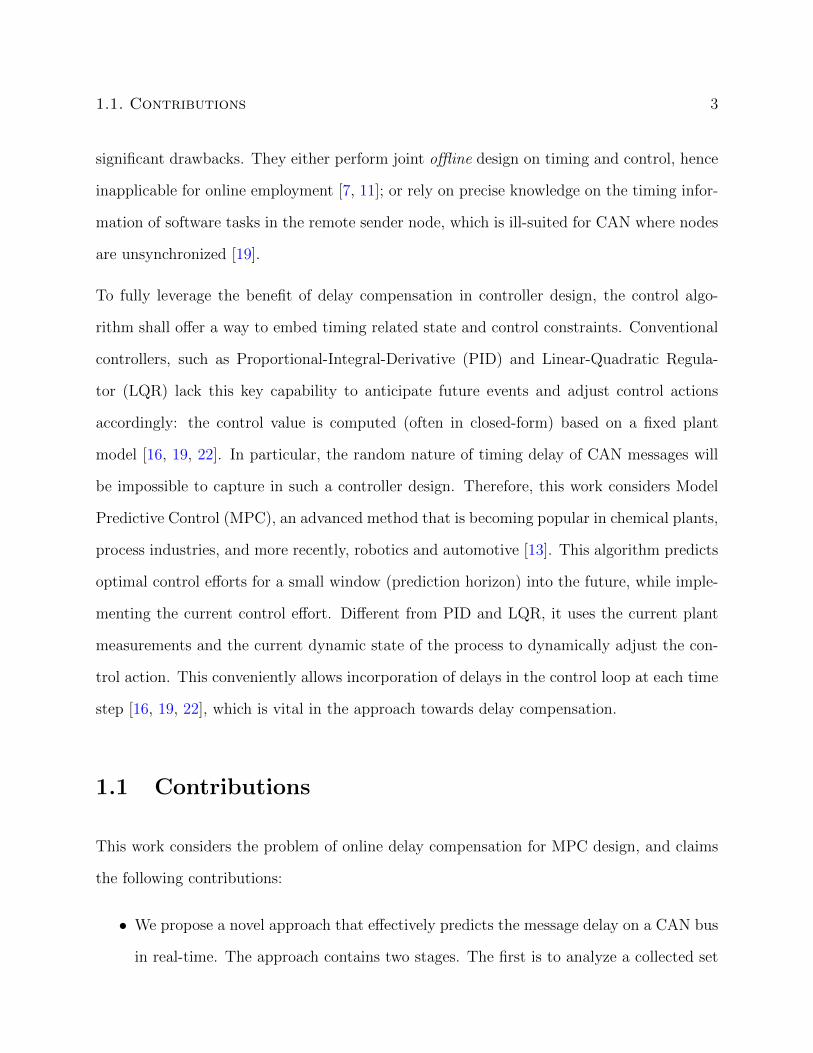
1.1 Contributions

This work considers the problem of online delay compensation for MPC design, and claims

the following contributions:

• We propose a novel approach that effectively predicts the message delay on a CAN bus

in real-time. The approach contains two stages. The first is to analyze a collected set

4 Chapter 1. Introduction

Figure 1.1: CAN based Control Systems with Feedback Loops with a proposed Delay Pre-dictor for Compensation

of traces (message reception events) and determine the nominal timing properties of

the messages, without assuming detailed knowledge on the sender nodes. The second

stage uses the results of the first stage to successfully predict the delay of every relevant

message in real-time.

• We also ensure its real-time feasibility by implementing the method and measuring its

worst-case execution time (WCET) on a low-end 8-bit microcontroller.

• We then include the timing information as constraints into the MPC controller design of

a Cruise Control system [2] and a DC servo [1], to demonstrate the control performance

improvement in terms of the rise time and maximum overshoot of the plant output.

The entire setup is represented by the block diagram shown in Figure 1.1.

Chapter 2

Review of Literature

With respect to controller design, the literature does offer quite a few works that perform

offline timing and control analysis together (e.g., [4, 5, 6, 7, 25]). However, as the name

suggests, offline methods lead to overly conservative designs, and they are unsuitable to be

employed in real-time as well as in conjunction with the MPC design [13, 19].These are

usually performed using computer simulations for all time stamps based on the employed

scheduling algorithm. As far as Model predictive control is concerned, these offline computer

simulations will prove too expensive. Online methods must design a schedule of events and

apply the control strategy at each sampling instant for the finite horizon. This saves a lot

of computation as compared to the offline strategies as we are optimizing only for a finite

window and not for all the samples.

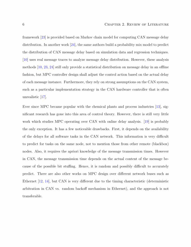
The timing delay of CAN messages has been studied in several contexts. Since CAN is typi-

cally used to support applications with hard real-time constraints, its worst-case delay (i.e.,

the maximum delay from its readiness to the completion of transmission) has been studied

in a variety of scenarios to make sure that the message deadline is met [8, 9, 15, 21]. How-

ever, this analysis only provides an upper bound on the message delay. A stochastic analysis

5

6 Chapter 2. Review of Literature

framework [23] is provided based on Markov chain model for computing CAN message delay

distribution. In another work [24], the same authors build a probability mix model to predict

the distribution of CAN message delay based on simulation data and regression techniques.

[10] uses real message traces to analyze message delay distribution. However, these analysis

methods [10, 23, 24] still only provide a statistical distribution on message delay in an offline

fashion, but MPC controller design shall adjust the control action based on the actual delay

of each message instance. Furthermore, they rely on strong assumptions on the CAN system,

such as a particular implementation strategy in the CAN hardware controller that is often

unrealistic [17].

Ever since MPC became popular with the chemical plants and process industries [13], sig-

nificant research has gone into this area of control theory. However, there is still very little

work which studies MPC operating over CAN with online delay analysis. [19] is probably

the only exception. It has a few noticeable drawbacks. First, it depends on the availability

of the delays for all software tasks in the CAN network. This information is very difficult

to predict for tasks on the same node, not to mention those from other remote (blackbox)

nodes. Also, it requires the apriori knowledge of the message transmission times. However

in CAN, the message transmission time depends on the actual content of the message be-

cause of the possible bit stuffing. Hence, it is random and possibly difficult to accurately

predict. There are also other works on MPC design over different network buses such as

Ethernet [12, 14], but CAN is very different due to the timing characteristic (deterministic

arbitration in CAN vs. random backoff mechanism in Ethernet), and the approach is not

transferable.

Chapter 3

Model Predictive Control

3.1 Overview

Simple lower order systems are often well controlled by simple PID controllers. When signif-

icant time delays are introduced in these systems, or when we have to deal with a system of

a very large order, it is considered very complex for a PID controller. Such systems require

the additional complexity and the predictive ability of the Model Predictive Control in a

controller in order to be controlled.

The main design objective of Model Predictive Control is to optimize the trajectory of the

future manipulated variable u (control effort) over a finite time window in order to optimize

the future performance output y of the plant. Unlike offline procedures, the MPC algorithm

performs predictions on-the-fly on the dependent variables based on the changes in the

independent variables of the system. The prediction is based on the past moves, the current

measurements, the current states of the variables and the constraints imposed on the output

- all in an effort to hold the dependent variables as close as possible to the target (or a

7

8 Chapter 3. Model Predictive Control

reference trajectory) in the near future. At each step, the algorithm uses an optimization

cost function J over the prediction horizon (H), to calculate the optimum control efforts.

This horizon keeps being shifted forward at every new step while the algorithm re-calculates

the new control effort. Because of this behavior, the horizon is also referred to as the receding

control horizon in the literature.

This can be understood of in terms of a day-to-day planning activity. Say we have to

prepare for an exam that is in 2 months. Initially, we optimally plan for the first 5 days and

implement the first day’s plan. Depending on how much of it we were able to implement

and how well we did, we re-plan for the next 5 days. This process is iterative until we reach

the target. At each step, we plan for the upcoming 5 steps while implementing the current

step, based on the prior progress, current state, while trying to stay as close to the optimal

plan.

3.2 Design Parameters

The key design parameters used in tuning the control performance are as follows:

• Sample Time(ts): This is the control interval duration and it is usually the parameter

that needs to be decided based on the application and held constant as the other

parameters are tuned.

It is important to recognize that as ts decreases, rejection of disturbances gets better at

the cost of the computation effort. It is vital to find the optimal balance of performance

and the computational effort needed.

• Prediction Horizon(H): The prediction horizon refers to the number of future control

intervals(ts) that the controller will predict by evaluation while optimizing its manip-

3.3. Delay Compensation in MPC Design 9

ulated variable(MV) at the current control interval.

Unfavorable plant characteristics combined with a small value of H can generate an

internally unstable controller. The remedy is to increase H if not large, but, if H is

already large, we’ll need to reconsider our ts or re think other parameters.

• Control Horizon(m): The control horizon refers to the number of MV moves to be

optimized at a given control interval. It lies between 1 and H.

Smaller values of m are preferred since it leads to fewer variables in the Quadratic Pro-

gram that needs to be solved at each control interval. This implies faster computation.

The MATLAB MPC Toolbox uses the KWIK algorithm to solve the QP [18].

3.3 Delay Compensation in MPC Design

The basic idea, as we know, in MPC is its iterative, finite-horizon optimization of the plant

model and the control action. At each time t it samples the current plant state, predicts the

changes in the other dependent state variables using online calculation, and computes a cost

minimizing control strategy (via a numerical minimization algorithm) for a (relatively short)

time horizon of length H, i.e., [t, t + H]. It then implements the first step of the control

strategy. For the next step, all the predictions are re-calculated over the prediction horizon,

yielding a new control effort. This happens over and over again whenever the controller is

triggered.

For simplicity, we use a single-input single-output linear time-invariant system to illustrate

the MPC design, but it can easily be extended to more sophisticated control systems. The

10 Chapter 3. Model Predictive Control

control system can be described by the equations

x(t) = Ax(t) +Bu(t); (3.1)

y(t) = Cx(t) (3.2)

where u(t) is the control effort at time t, y(t) is the output of the system, x(t) is the plant

state, and A, B, and C are constant.

In the control implementation, the sensor senses the status of the plant x(t) and triggers the

controller. The controller uses the sensed information and generates a control signal u(t)

every time it is triggered. Since the sensed data and the control signal may need to transmit

over the CAN bus, there exists a lag from the moment when the sensor measures the plant

states, to the moment when the actuator executes the control signal.

The computed control signal u(t) is applied to the plant until the next sensor message triggers

the controller [19]. Thus, the control effort u(t) in Equation (3.1) is a piecewise constant

function:

u(t) = µ[k], t ∈ [as,k + δk, as,k+1 + δk+1] (3.3)

where as,k is the k-th sampling instant of the sensor, µ[k] is a constant, δk is the delay that

exists between the time of sampling as,k and the reception time tu,k of µ[k], i.e., δk = tu,k−as,k.

In MPC, the prediction time horizon for the k-th sampling is [as,k, as,k + H]. The goal is

to find a control command u(t) that minimizes the difference between the predicted plant

output y(t) and the reference trajectory r(t) over the whole prediction horizon. In the control

design, a cost function models the impact of various parameters in the effort of the controller

to track the reference signal r(t). Weights (or penalties) are assigned to the involved variables

to penalize the controller for violating the associated constraints. The designed cost function

3.3. Delay Compensation in MPC Design 11

is then optimized to output the optimal control effort un(t). A typical and suitable example

cost function is [18, 19]

J(x(t), u(t))

=

∫ as,k+H

as,k

{(r(s)− y(s))T ·Q1 · (r(s)− y(s)) + u(s)T ·Q2 · u(s)

}ds

+xT (as,k +H) ·Q3 · x(as,k +H)

(3.4)

where Q1, Q2 and Q3 are non-negative constants (weights/penalties).

The objective is to minimize the above cost function subject to the constraints put forth in

the plant model in Equations (3.1)–(3.3). Thus the design of the MPC control requires the

values for δk in the prediction horizon.

However, in CAN, numerous messages from various unsynchronized computing nodes con-

tend to access the medium. Time-variant message delays are introduced, since the clocks

of computing nodes are randomly drifting, and consequently the time that messages are

ready for bus contention is random. Therefore, it is challenging to obtain the δk predictions

accurately and in an online fashion, which the next chapter will address.

Chapter 4

Online Delay Prediction on CAN

The purpose of having a timing model is to explicitly define and discuss the kind of timing

properties that the CAN bus can inject into the system. This will help in predicting timing

faults or non-ideal timing behaviors for all the CAN messages and will help in overcoming

them. In this chapter, we will discuss the CAN timing model, and the algorithm which

predicts message delays and outputs it to the MPC for delay compensation. Our approach

is based on two of simple characteristics in CAN.

The first is that the CAN arbitration protocol is both priority-based and non-preemptive.

Priority-based means that when multiple nodes with ready messages try to access the shared

bus medium, the node sending the message with lowest identifier is always the winner of the

arbitration round and is transmitted next. Hence, in CAN, each message is assigned with

a unique identifier (which is referred to as unique purity), and the lower the identifier, the

higher the priority. Non-preemptive means that a message being transmitted can not be

preempted by higher priority messages that are made available after the transmission has

started.

12

13

TxTask

Signal variables

periodicactivation

Messagequeue

Middleware

Driver

(priority−based arbitration)CAN bus

Figure 4.1: CAN System architecture.

In addition, we observe that sensor data are periodically sampled in control systems . Hence,

in most implementations of CAN, there is a software task in the middleware layer, called

TxTask, which is periodically activated and responsible for packing messages from signal

data and queuing them for transmission [11]. This is supported by the automotive AU-

TOSAR/OSEK standard and implemented by the commercial tools from Vector [3]. In

other words, this TxTask synchronizes the queuing of all messages from the same node. A

representation of the CAN system architecture is shown in Figure 4.1.

For the purpose of timing analysis, each periodic message stream mi is characterized by the

tuple

mi = {idi, Li, Ti}

where Li is the data content in bits, idi is the CAN identifier, and Ti is its period. CAN

messages can only contain a data content that is an integer multiple of 8 bits. The actual

message length needs to account for the protocol bits in addition to the data content, in-

cluding stuffed bits (34 of the 46 protocol bits are subject to stuffing) that are dependent on

14 Chapter 4. Online Delay Prediction on CAN

the data content.

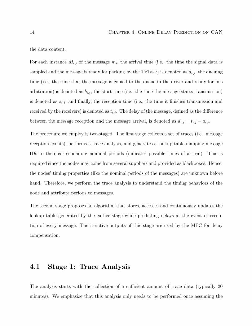
For each instance Mi,j of the message mi, the arrival time (i.e., the time the signal data is

sampled and the message is ready for packing by the TxTask) is denoted as ai,j, the queuing

time (i.e., the time that the message is copied to the queue in the driver and ready for bus

arbitration) is denoted as bi,j, the start time (i.e., the time the message starts transmission)

is denoted as si,j, and finally, the reception time (i.e., the time it finishes transmission and

received by the receivers) is denoted as ti,j. The delay of the message, defined as the difference

between the message reception and the message arrival, is denoted as di,j = ti,j − ai,j.

The procedure we employ is two-staged. The first stage collects a set of traces (i.e., message

reception events), performs a trace analysis, and generates a lookup table mapping message

IDs to their corresponding nominal periods (indicates possible times of arrival). This is

required since the nodes may come from several suppliers and provided as blackboxes. Hence,

the nodes’ timing properties (like the nominal periods of the messages) are unknown before

hand. Therefore, we perform the trace analysis to understand the timing behaviors of the

node and attribute periods to messages.

The second stage proposes an algorithm that stores, accesses and continuously updates the

lookup table generated by the earlier stage while predicting delays at the event of recep-

tion of every message. The iterative outputs of this stage are used by the MPC for delay

compensation.

4.1 Stage 1: Trace Analysis

The analysis starts with the collection of a sufficient amount of trace data (typically 20

minutes). We emphasize that this analysis only needs to be performed once assuming the

4.1. Stage 1: Trace Analysis 15

Reception ID Data Content Arrival Start Delay REF1145332 1C1 03 45 03 4C 1144241 1145150 10911148042 0C1 20 04 7C 82 20 11 BF 37 1147679 1147802 363 YES1148282 0C5 20 13 FB 69 20 0E 9F B8 1147679 1148042 6031148532 0F9 00 00 40 00 00 00 03 FF 1148201 1148282 3311148765 199 CF FF 0E 70 F1 8D 00 FF 1148201 1148532 5641148999 1E5 46 05 6C E0 00 FA 91 00 1147679 1148765 13201149185 2F9 C8 01 0F 00 00 1147679 1148999 15601149357 348 00 00 00 00 1147679 1149185 16781149531 34A 00 00 00 00 1147679 1149357 18521151167 0F1 1C 02 00 40 1150810 1150981 357 YES

Table 4.1: Trace segment from a production vehicle, with computed arrival time, start time,and delay (time unit: µs).

message nominal periods remain the same.

In the message trace, each line depicts an event of successful message reception on the bus.

The trace T consists of a finite sequence of events ei, T = {e0, e1, . . . , en}, where each event

ei is a tuple that includes the event time stamp (i.e., the time the message successfully

transmitted on the bus and received by all other nodes), the CAN ID of the message to

which the event is referred, and the data content which implicitly gives the corresponding

total number of bits (including stuff-bits). By studying the trace T we can extract an

estimate of information about a (possibly blackbox) node, including:

• The reconstruction of the possible message arrival time and delay starting from its

reception time stamp;

• The detection of true message periods;

• The analysis of the scheduling delays of TxTask.

As an example, a segment of the trace collected from a production vehicle and the analyzed

message delay are provided in Table 4.1, where the first three columns are the reception time

stamp, message ID, and the data content. The bus speed is 500kbps, hence, the message

transmission time is between 94µs (microseconds) to 270µs.


transmission time

ideal periodic activation of Txtask for message enqueuing

reception timestart timequeuing time next arrival timearrival time

Scheduling delay(TxTask)

queuing delay

Figure 4.2: From message arrival to message reception.

The reconstruction of the message arrival times is based on their reception times. This is

done by backtracking in time and subtracting the factors that contribute to the total message

delay, as illustrated in Figure 4.2. Specifically, the message delay di,j = ti,j−ai,j of a message

instance Mi,j is composed of three components:

• The scheduling delay of the TxTask, i.e., (bi,j − ai,j). At the end of the TxTask

execution, the message is queued to the hardware buffer and ready for arbitration.

• The queuing delay (si,j−bi,j), i.e., the time from its queuing to its start of transmission.

• The message transmission time (ti,j − si,j), i.e., the time between its start of transmis-

sion to its reception.

The message transmission time is easy to calculate from the trace, as it is simply the quotient

of the the number of bits in the message (including stuff-bits that are added depending on the

data content) divided by th bus speed (how many bits are transmitted each second). Since

CAN is non-preemptive, the start time is derived by subtracting the message transmission

time from ti,j.

The queuing delay and the TxTask scheduling delay depend on the other tasks and messages

in the system, and are more challenging to find out. We observe that the queuing delay is


generally unknown (as how much a message is delayed by messages of other unsynchronized

nodes is unknown), except for a few reference events for which it can be neglected. Specifi-

cally, for each event in the trace, if the calculated start time does not overlap (i.e., separated

by a safe distance to account for possible imprecision in the recorded time) with the recep-

tion time of the previous event, a bus idle time interval between the two events is identified.

The message that is transmitted after the idle time is labeled as a reference event with zero

queuing delay.

Base rate messages : Messages from the same node are almost always enqueued with har-

monic periods by a dedicated task (on middleware). This supports the assumption we made

clear earlier. Therefore, every instance of tasks with harmonic periods on a node is bound to

be launched on the bus with another task, thus delaying one of them based on priority. Thus

we define a base rate message as that which runs on each node with a period = (gcd) of the

periods of the messages and has the highest local priority. Hence, the base rate message acts

as a reference of the arrival times of all the other messages since every message is launched

with one of the instances of the base-rate message. This relation between the arrival times

is used for the reconstruction of arrival times of all messages as we will show.

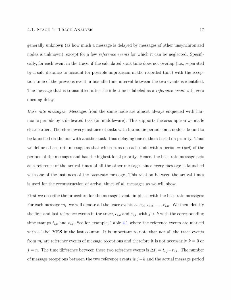
First we describe the procedure for the message events in phase with the base rate messages:

For each message mi, we will denote all the trace events as ei,0, ei,2, . . . , ei,n. We then identify

the first and last reference events in the trace, ei,k and ei,j, with j > k with the corresponding

time stamps ti,k and ti,j. See for example, Table 4.1 where the reference events are marked

with a label YES in the last column. It is important to note that not all the trace events

from mi are reference events of message receptions and therefore it is not necessarily k = 0 or

j = n. The time difference between these two reference events is ∆ti = ti,j−ti,k. The number

of message receptions between the two reference events is j−k and the actual message period


REF

i,k~

a i,q*~ a i,q*

a i,k a i,j

t i,k t i,q* t i,j

iT

a i,j~=

REF REF

a

Figure 4.3: Finding the reference event with the smallest TxTask scheduling delay.

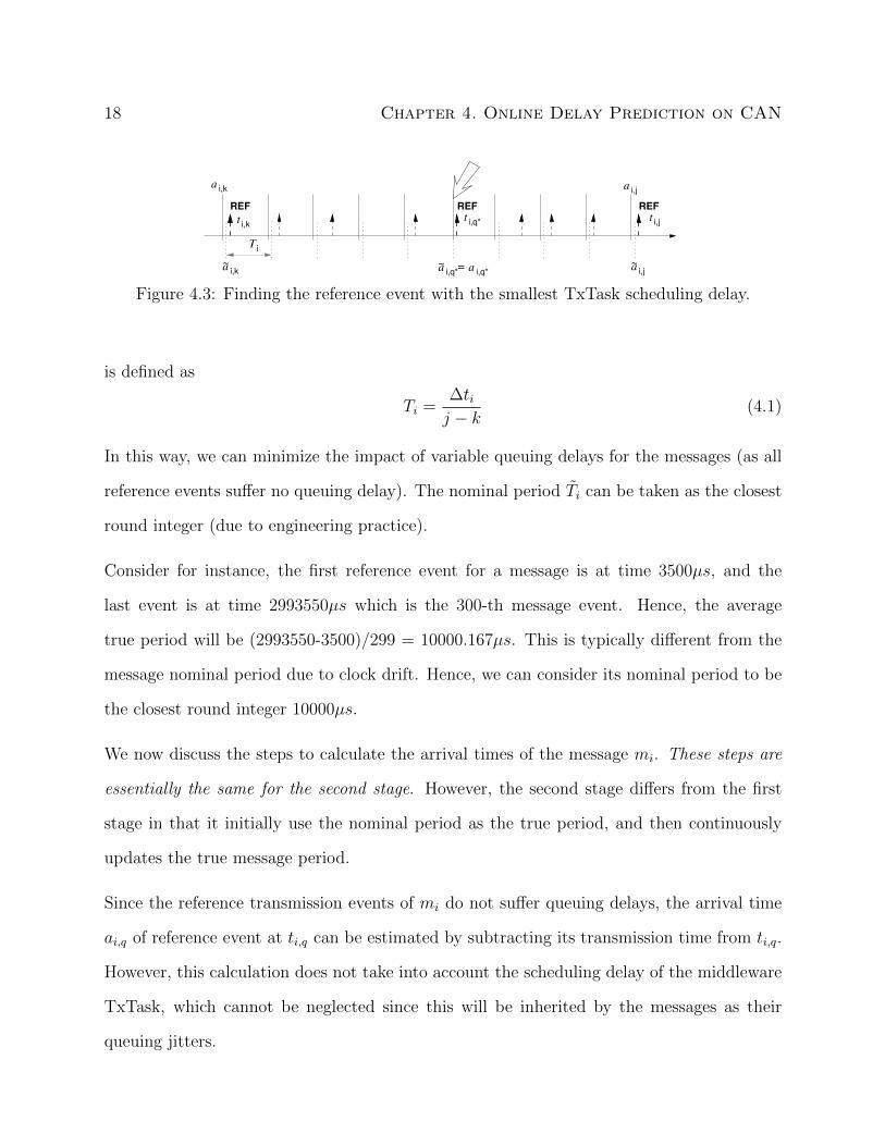
is defined as

Ti =∆tij − k

(4.1)

In this way, we can minimize the impact of variable queuing delays for the messages (as all

reference events suffer no queuing delay). The nominal period Ti can be taken as the closest

round integer (due to engineering practice).

Consider for instance, the first reference event for a message is at time 3500µs, and the

last event is at time 2993550µs which is the 300-th message event. Hence, the average

true period will be (2993550-3500)/299 = 10000.167µs. This is typically different from the

message nominal period due to clock drift. Hence, we can consider its nominal period to be

the closest round integer 10000µs.

We now discuss the steps to calculate the arrival times of the message mi. These steps are

essentially the same for the second stage. However, the second stage differs from the first

stage in that it initially use the nominal period as the true period, and then continuously

updates the true message period.

Since the reference transmission events of mi do not suffer queuing delays, the arrival time

ai,q of reference event at ti,q can be estimated by subtracting its transmission time from ti,q.

However, this calculation does not take into account the scheduling delay of the middleware

TxTask, which cannot be neglected since this will be inherited by the messages as their

queuing jitters.


We notice that the arrival times must come at a periodic base due to the periodic activation

of TxTask. Hence, starting from the first reference event at ti,k, with the value of true period

Ti estimated, the arrival times are also estimated using ai,q = ai,k + Ti × (q − k) (shown as

dotted lines in Figure 4.3).

Then, we find the reference event with the smallest TxTask scheduling delay and use it as

the base for arrival time calculation. More specifically, for all the reference events ei,q for

message mi, the value li,q = ai,q − ai,q is computed, and the one ei,q∗ with the smallest li,q

indicates the case suffering the smallest TxTask scheduling delay. The minimum value

Ja∗i = minq{li,q} (4.2)

(which shall be negative) is then applied as a correction to obtain the estimated arrival times

ai,q = ai,q + Ja∗i .

In Figure 4.3, a minimum value Ja∗i is obtained for the event indicated by the arrow, and the

arrival times are shifted left to the solid lines, yielding the final result. As in the figure, the

corrected arrival times ai,q are equal to ai,q for the event ei,q∗ , and for the other events it is

ai,q < ai,q. The (ti,q − ai,q) values for all the reference events from the same node is assumed

as the queuing jitter, i.e., the scheduling delay of the TxTask.

For message events that arrive at with a phase difference with respect to the base rate mes-

sages, we first find the phase associated with each of them and then assign the corresponding

arrival times. The following procedure detects the phases of such messages on a node in ref-

erence to the base rate message and then assigns arrival times based off of the results. The

method is hinged on the initial assumption that the majority of the message instances are

transmitted with a response time lower than the period of the base message. This assump-

tion is valid in most cases and exceptions can be detected a posteriori and corrected. The


mul[i]=2i=0count[] = {3, 1}

0 1 2 3 4 5 6 7

baseIx % mul[i] =

baseIx = 2 baseIx = 5

baseIx % mul[i] =

baseIx = 6

baseIx % mul[i] =

Base message index

baseIx

baseIx = 0

baseIx % mul[i] = 0 0 1 0

φ

Figure 4.4: Detection of the message phase

procedure is formally described in Algorithm 1, and an example is provided in Figure 4.4.

An index baseIx is assigned to each instance of the base message, starting with 0. An array

mul[] is defined to store the period ratio of all the other messages and the base rate message,

one entry per message.

Algorithm 1 Calculate phase φi of ei,j1: for each trace event e = ei,j do2: Message m = e.GetMessage();3: ECU c = m.GetEcu();4: Message bm = e.GetBaseRateMessage();5: if bm == m then6: c.SetBaseCount(index);7: else8: ph = c.GetBaseCount() % m.GetMultiplier();9: m.phase count[ph]++;

10: end if11: end for12: for each message m = mi do13: m.phase = Index of max(m.phase count);14: end for

The minimum response time of message mi can be calculated as the minimum queuing delay

caused due to the higher priority messages on the same node which are always queued before

mi, added to the transmission time of mi itself. Next, the phase of the message should is

adjusted such that the analyzed response time in the trace should always be larger than its

calculated minimum response time. An array of counters phase count[] of size mul[i] is

defined for each message. For every instance of mi with period larger than the base period,


the algorithm finds the value of baseIx for the latest transmission of the base message and

computes val=baseIx % mul[i]. Then, the counter in phase count[] which matches val

is incremented. By the end of this, the index of the counter array with the largest value is

output as the phase φi of the message.

Algorithm 2 Calculate arrival time of ei,j1: for each trace event e = ei,j do2: Message m = e.GetMessage();3: ECU c = m.GetEcu();4: Message bm = e.GetBaseRateMessage();5: if bm == m then6: c.SetBaseCount(index);7: c.SetLastBaseArrival(e.GetArrivalTime());8: else9: mcnt = m.GetBaseDynCnt();

10: bcnt = c.GetBaseCount();11: m.SetBaseDynCnt(mcnt + m.GetMultiplier());12: ∆ = bcnt-mcnt;13: if ∆ < 0 then14: ∆ = ∆ + m.GetMultiplier();15: end if16: e.SetArrivalTime(c.GetLastBaseArrival() - ∆×bm.GetTPeriod();17: end if18: end for

In the example illustrated by Figure 4.4, four transmission events return a phase count equal

to 0 and only one returns a phase count of 1. Therefore, the algorithm outputs φi = 0 and

assigns the corresponding arrival time by back-tracking until the first event of the base rate

message with index k×mul+ φi, where k ∈ 0, 1, 2, . . . is encountered. If such an event does

not exist, i.e., the base rate transmission of index φi occurs after the message transmission

event in question (the one that the algorithm is considering), then the arrival time of the

base rate event with index φi is decremented by the period of the message and assigned as

the message arrival time. This is formally described as Algorithm 2.


4.2 Stage 2: Delay Prediction

Before the delay compensation is in effect, the system is first subject to the trace analysis

described in the above subsection. This will populate a lookup table with message IDs and

the nominal message periods. This step only needs to be carried out once, unless the nominal

periods of messages change.

The delay prediction stage calculates the message delay for each message mi following the

same principle of Section 4.1, except that

• the message true period shall be updated each time it encounters a reference event of

the message, to adjust it according to the actual clock speed of the nodes;

• the reference event q∗ with the smallest TxTask scheduling delay shall be updated

whenever a smaller Ja∗i is observed.

We will need to keep updating the Ti values with time. As and when a new message arrives

into the predictor, its nominal time period Ti is looked up from the table. The difference

between the nominal arrival time and the actual time of arrival of the message is returned as

the delay δk. These delays are aggregated and stored in an array delaytracker, one index per

message id. Another array (dynCount) maintains the current count indicating the number

of times each message has arrived up to that point. The look up table id updated after the

occurrence of a Reference event. The aggregated delay value for every message is divided

by the number of occurrences in that reference window and added to the Ti corresponding

to the msgID in the look-up-table. The aggregate delay array is then reset. Thus, the

predictions of arrival times get closer and closer to the accurate value, thereby reducing the

delay in every feedback loop with time.

The procedure is formalized in Algorithm 3. In the main loop of execution, we maintain two

4.2. Stage 2: Delay Prediction 23

Algorithm 3 Calculate and predict δk for every incoming message mi,j

1: for each incoming message m = mi,j do2: r = nextReferenceInstance;3: if (m == r) then4: updateTPs(delaytracker,dynCount);5: reset.dynCount;6: reset.delaytracker;7: end if8: delay=calculateDelay(m,count,delaytracker,dynCount);

//delay is given as the input to the MPC9: end for

//Functions:10: calculateDelay:

index = find(msgId == id);cnt[index] = cnt[index] +1;DynCount[index] = DynCount[index] + 1;expected arr = cnt[index] x T [index];delay = time - expected arr;delayTracker(index)=delayTracker(index)+delay;

end11: updateTPs:

for each Ti entry in the lookuptable dooffset={DelayTracker[i]/(DynCount[i]+1)};Ti = Ti + offset ;

end forend

functions: calculateDelay and updateTPs. For every new message msgIn that arrives into

the predictor, we call the calculateDelay function which returns the delay estimate for that

particular message. We also check if the event is a reference event (message transmission

with no queuing delay). If so, we call updateTPs by passing the arrays delaytracker and

counter array dynCount.

The function calculateDelay looks up the message’s Time Period, calculates the next pre-

diction for the arrival time, and returns the difference as the delay. It also maintains the

counters count and DynCount by incrementing the count in the index corresponding to the

message ID.

The function updateTPs, updates the T column in the lookup table for all the messages.

This is done by averaging the aggregated delay (stored in delayTracker) for each message


Message ID T0x02 400x01 200x00 10

Table 4.2: Initial lookup table for the Example with N = 3

Message ID T0x02 40.340x01 20.250x00 9.63

Table 4.3: Updated lookup table for the Example with N = 3 after 2 reference events

over the number of times each message arrived in that window (stored in DynCount).The

window is refreshed in the main loop soon after updateTPs is called upon.

Table 4.2 shows the initial lookup Table (result of the offline trace analysis, say) for a toy

example with 3 messages in the lookup. The experiment is conducted on a hardware which

implements the online algorithm, and Table 4.3 shows the updated lookup table after 38

message events out of which 2 were reference message events. The algorithm considers the

higher message ID to have the higher priority (0x02 in this case). Therefore, as it can be seen

from the table, the message 0x00 acts as the base rate message for this particular ECU. The

second and fourth instances of 0x02 are identified as the reference instances of the highest

priority message on this ECU. Therefore, the table 4.3 shows the lookup table after two

updates (once for every reference event). Figure 4.5 also shows a snapshot the Arduino

Serial port console. We can see the delay values being predicted for every message and the

lookup updated upon detection of a reference event.

Now we are fully equipped to solve the problem posed in Section 3.3 since we have the needed

information for calculating δk within the prediction horizon. Specifically, δk is the difference

between the arrival of the sensor message instance as,k and the reception of the actuator

message tu,k. Hence, the controller, once receiving the sensor message, can calculate the

arrival time as,k using the approach developed in this section. Once the actuator message

4.2. Stage 2: Delay Prediction 25

Figure 4.5: Serial Port Console showing online delay predictions and LookUp Updations


is transmitted, the time stamp tu,k is recorded, and the delay δk for the control loop is

calculated as tu,k − as,k. These values then will be used for predicting the future delays.

Chapter 5

Experimental Results

In this section, we present our experimental results. Specifically, we verify that our online

delay prediction algorithm is in fact capable of performing the computations in real-time,

as it has small runtime overhead. We also motivate the need of online delay prediction by

analyzing the error incurred by clock drifts on delay calculation. We then use two example

control systems to demonstrate the effectiveness of the delay compensation.

5.1 Measurement of Online Algorithm Timing Over-

head

To ensure that our online delay prediction algorithm is actually feasible, we implement it

and measure the timing overhead. We use an Arduino Uno board which houses a low-end,

8-bit, 16 MHz ATmega328P controller. We used a CAN Shield to provide CAN capabilities

to the microcontroller. This CAN Shield adopts a MCP2515 CAN Bus controller with SPI

interface and MCP2551 CAN transceiver [20]. The experimental setup we used is as follows:

27

28 Chapter 5. Experimental Results

We use two Arduinos A and B; each connected to a different serial port on the same machine

or one serial port on two different machines. A and B are connected via CAN. A sends over

messages with different message IDs every 50 milliseconds on the CAN. B receives these

messages and represents the delay predictor box. This means that B stores the lookup table

that results from the offline trace analysis and performs the computation of the delays in

real-time as and when the message is received over CAN from A, updates the lookup, etc. It

is helpful to note that the delay prediction algorithm on B does not deal with growing data

structures for a given system.

0 1 2 3 4 5 6 7 80

50

100

150

200

250

300

350

400

450

Number of messages

WC

ET

[µs]

Figure 5.1: WCET trend with increasing number of messages.

We measure the worst-case execution time (WCET) of stage 2 (i.e., the stage after the nom-

inal period is constructed). As in Figure 5.1, the WCET of the proposed method increases

almost linearly with the number of messages. As a general trend, it can be observed that

every message adds around 48µs to the WCET. This is significantly smaller than the typical

period of control loop (in the range of tens of milliseconds to several seconds), and thus the

algorithm is feasible for real-time delay prediction.

5.2. Necessity of Online Delay Prediction 29

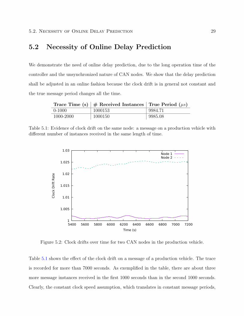
5.2 Necessity of Online Delay Prediction

We demonstrate the need of online delay prediction, due to the long operation time of the

controller and the unsynchronized nature of CAN nodes. We show that the delay prediction

shall be adjusted in an online fashion because the clock drift is in general not constant and

the true message period changes all the time.

Trace Time (s) # Received Instances True Period (µs)0-1000 1000153 9984.711000-2000 1000150 9985.08

Table 5.1: Evidence of clock drift on the same node: a message on a production vehicle withdifferent number of instances received in the same length of time.

1

1.005

1.01

1.015

1.02

1.025

1.03

5400 5600 5800 6000 6200 6400 6600 6800 7000 7200

Clo

ck D

rift

Rate

Time (s)

Node 1Node 2

Figure 5.2: Clock drifts over time for two CAN nodes in the production vehicle.

Table 5.1 shows the effect of the clock drift on a message of a production vehicle. The trace

is recorded for more than 7000 seconds. As exemplified in the table, there are about three

more message instances received in the first 1000 seconds than in the second 1000 seconds.

Clearly, the constant clock speed assumption, which translates in constant message periods,


cannot be sustained. Otherwise, the predicted message delay will be constantly growing,

which reaches about three times of its period (period is approximately 10 ms) i.e., about

30 milliseconds, as opposed to the actual delay that is always below 1 millisecond after the

system operates for 2000 seconds.

Figure 5.2 shows the measured clock drifts of two different nodes in the same vehicle. The

clock drift is calculated as the ratio between the message true period and its nominal period.

It is evident that the clocks of different nodes are generally drifting at different speeds all the

times. Hence, even if the nominal message periods are known apriori, it is still necessary to

continuously compute the true periods in an online fashion to avoid accumulating the error.

5.3 MPC Performance

Next, to simulate the control system and evaluate the performance of the controller delay

compensation, we use the Model Predictive Control Toolbox on MATLAB in a CAN envi-

ronment provided by TrueTime [6]. It is a simulator software for real-time control systems

that works with MATLAB and Simulink. We apply the delay prediction method to two

example systems. One is a cruise control system described in [2], the other is a DC servo [1].

In the cruise control system [2], the vehicle mass (m) is set to 1000kg, the damping coefficient

(b) is 50Ns/m, and the nominal control force is 500N. It is assumed that rolling resistance and

air drag are proportional to the car’s speed. The control system equation in the state-space

form is

[v] =

[−bm

][v] +

[1

m

][u] (5.1)

y =

[1

][v] (5.2)

where v is the velocity of the car which is also the output state.

5.3. MPC Performance 31

The DC Servo, found in the Truetime Library [1], has the following state equations:

[x] =

−50 0

1 0

[x] +

[1 0

][u] (5.3)

[y] =

[0 1000

][x] (5.4)

We inject delays in the system for both the actuator message (from controller to actuator)

and the sensor message (from sensor to controller). To match the actual implementation of

CAN systems, the message trace used to inject delay in the control system is recorded from

a CAN bus in a production vehicle.

0 2 4 6 8 10

-1

-0.5

0

0.5

1

Ref Trajectory

CC Output

Overshoot

Tr

Figure 5.3: A sample output explaining the concepts of rise time and overshoot.

Figure 5.3 shows a sample output of the cruise control plant for a particular MPC design

with online delay prediction. The y-axis shows the plant output y(t) against time t on the

x-axis. The black solid line represents the plant output and the red dashed line denotes the

reference trajectory. We are interested in comparing the rise time (i.e., the time needed to


400 500 600 700 800 900 1,0001,100

1.2

1.6

2

2.4

2.8

3.2

+/- Constraints

Ris

eT

ime

[s]

No PredictionOnline Prediction

(a) Rise Time (Tr) for various constraints on con-trol effort u(t).

400 500 600 700 800 900 1,0001,1000

0.1

0.2

0.3

0.4

0.5

+/- Constraints

Ove

rshoot


(b) Overshoot for various constraints on controleffort u(t).

Figure 5.4: MPC control performance for cruise control system.

meet the changing trajectory), and the maximum overshoot (the amount the control output

exceeding its reference) against MPC designs for (i) no delay prediction and (ii) online

prediction timing model.

The observed rise time and overshoot are plotted in Figures 5.4 and 5.5 respectively. Here


4 5 6 7 8 9

·10−2

0

0.2

0.4

0.6

0.8

1

1.2

1.4

1.6

1.8

2

+/- Constraints

Ris

eT

ime

[s]


(a) Rise Time (Tr) for various constraints on Con-trol Effort u(t).

4 5 6 7 8 9

·10−2

0

5 · 10−2

0.1

0.15

0.2

0.25

0.3

0.35

+/- Constraints

Ove

rshoot


(b) Overshoot for various constraints on controleffort u(t).

Figure 5.5: MPC control performance for DC servo.

the x-axis represents the applied constraints on the control effort in the MPC Design. For

example, in Figure 5.4, 800 represents a constraint of +/- 800N on the Force in the cruise

control. It is important to note that a higher value on the x-axis indicates a less constrained


control design.

From the figures 5.4 and 5.5, we can see that having the online prediction timing model

reduces the rise time at the cost of maximum overshoot. As per the application, the designer

can decide on a trade-off between the rise-time and the corresponding overshoot to decide on

the appropriate constraint on the control effort. The other observation is that, as we go on

reducing the constraint on the the control effort, the overshoot increases, thereby decreasing

the rise time. Similar trend is observed with the DC Servo plant (plotted in Figures 5.5a

and 5.5b), where the x-axis has different scales since the plant is different.

Finally, Figures 5.6 and 5.7 respectively show a sample plant output of the Cruise Control

and the DC Servo plant while tracking a square trajectory. The y-axis shows the plant output

y(t) against time t on the x-axis. In the subfigure (a), the output is based on inaccurate

predictions of δk using the worst-case message delay, and the subfigure (b) shows the output

with the online delay prediction. The DC Servo output is evidently better with accurate

predictions than the one with inaccurate predictions. We can see the output growing in

amplitude with increasing overshoots above the reference trajectory. We also confirmed

that the worst case predictions have rendered the system unstable by using the ”isstable”

command on MATLAB. The same system is held stable and tracks the reference better when

our prediction algorithm is used. The cruise control plant output is stable in both cases,

but the performance and reference tracking is noticeably better in Figure 5.6b compared to

Figure 5.6a. With inaccurate worst-case delay predictions, the rise time is higher than with

accurate predictions. This also confirms the results presented in Figures 5.4 and 5.5.


0 5 10 15 20

-1

-0.5

0

0.5

1

CC Output

Reference

(a) Inaccurate prediction with worst-case delay.

0 5 10 15 20

-1

-0.5

0

0.5

1

Reference

CC Output

(b) Prediction with our method.

Figure 5.6: MPC control output with two different prediction methods of δk for cruise controlsystem.


0 5 10 15 20

-2

-1

0

1

2

Servo Output

Reference

(a) Inaccurate prediction with worst-case delay.

0 5 10 15 20

-1.5

-1

-0.5

0

0.5

1

Reference

Servo Output

(b) Prediction with our method.

Figure 5.7: MPC control output with two different prediction methods of δk for DC servo.

Chapter 6

Conclusions

This work studies the problem of online delay prediction for control systems design in CAN-

based Cyber-Physical Systems. The main contribution of this work is the timing model

with online delay prediction algorithm for messages scheduled on a CAN bus. It assumes no

detailed knowledge on the other computing nodes. It leverages the characteristic of CAN,

and finds a special kind of message reception events, to backtrack from the message reception

to the message arrival and calculate the message delay. The work then demonstrates that

the online delay prediction is in fact feasible to be deployed in a real-time scenario by

implementing it and measuring the Worst-Case Execution Time (WCET). Such a delay

prediction method is then applied to the design of the model predictive control algorithm.

The work analyzes the rise time and maximum overshoot of the control output, to illustrate

the benefit of the proposed method.

37

Bibliography

[1] TrueTime: Simulation of Networked and Embedded Control Systems. [Online]

http://www.control.lth.se/truetime/.

[2] Control Tutorials for MATLAB and Simulink - Cruise Control: System Modeling. [On-

line] http://ctms.engin.umich.edu/CTMS/.

[3] Vector CANbedded: OEM-Specific Embedded Software Components for CAN Commu-

nication in Motor Vehicles. [Online] https://vector.com/vi canbedded en.html.

[4] A. Anta and P. Tabuada. On the benefits of relaxing the periodicity assumption for

networked control systems over can. In 30th IEEE Real-Time Systems Symposium, 2009.

[5] K.-E. Arzen, A. Cervin, J. Eker, and L. Sha. An introduction to control and scheduling

co-design. Proceedings of the 39th IEEE Conference on Decision and Control, pages

4865–4870, 2000.

[6] A. Cervin, D. Henriksson, B. Lincoln, J. Eker, and K.-E. Arzen. How does control timing

affect performance? analysis and simulation of timing using jitterbug and truetime.

IEEE Control Systems, 23(3):16–30, 2003.

[7] Thidapat Chantem, Xiaobo Hu, and M.d. Lemmon. Generalized elastic scheduling. 27th

IEEE International Real-Time Systems Symposium, 2006.

38

BIBLIOGRAPHY 39

[8] R. Davis, A. Burns, R. Bril, and J. Lukkien. Controller area network (can) schedulability

analysis: Refuted, revisited and revised. Real-Time Systems, 35(3):239–272, 2007.

[9] R. Davis, S. Kollmann, V. Pollex, and F. Slomka. Controller area network (can) schedu-

lability analysis with fifo queues. In 23rd Euromicro Conference on Real-Time Systems,

pages 45–56, 2011.

[10] M. Di Natale and H. Zeng. System identification and extraction of timing properties

from controller area network (can) message traces. 15th IEEE Conference on Emerging

Technologies & Factory Automation, (4), 2010.

[11] Marco Di Natale, Haibo Zeng, Paolo Giusto, and Arkadeb Ghosal. Understanding and

using the controller area network communication protocol: theory and practice. Springer,

2014.

[12] G. Goodwin, H. Haimovich, D. Quevedo, and J. Welsh. A moving horizon approach

to networked control system design. IEEE Transactions on Automatic Control, 49(9):

1427–1445, 2004.

[13] J. Lee, M. Morari, and C. Garcia. State-space interpretation of model predictive control.

Methods of Model Based Process Control, pages 299–330, 1995.

[14] G. Liu, Y. Xia, J. Chen, D. Rees, and W. Hu. Networked predictive control of systems

with random network delays in both forward and feedback channels. IEEE Transactions

on Industrial Electronics, 54(3):1282–1297, 2007.

[15] Meng Liu, M. Behnam, and T. Nolte. An evt-based worst-case response time analysis

of complex real-time systems. In 8th IEEE International Symposium on Industrial

Embedded Systems, pages 249–258, June 2013.

40 BIBLIOGRAPHY

[16] D. Mayne, J. Rawlings, C. Rao, and P. Scokaert. Constrained model predictive control:

stability and optimality. Automatica, 36(6):789–814, 2000.

[17] M. Di Natale and H. Zeng. Practical issues with the timing analysis of the controller

area network. In 18th IEEE Conference on Emerging Technologies Factory Automation,

Sept 2013.

[18] C. Schmid and L. Biegler. Quadratic programming methods for reduced hessian sqp.

Computers & Chemical Engineering, 18(9):817–832, 1994.

[19] Z. Shi and F. Zhang. Model predictive control under timing constraints induced by

controller area networks. Real-Time Systems, 53(2):196–227, 2016.

[20] Seeedstudio Team. CAN-BUS Shield V1.2. [Online] http://wiki.seeed.cc/CAN-

BUS Shield V1.2/.

[21] K. Tindell, A. Burns, and A. Wellings. Calculating controller area network (can) mes-

sage response times. Control Engineering Practice, 3(8):1163–1169, 1995.

[22] Liuping Wang. Model predictive control system design and implementation using MAT-

LAB. Springer, London, 2010.

[23] H. Zeng, M. Di Natale, Paolo Giusto, and A. Sangiovanni-Vincentelli. Stochastic anal-

ysis of can-based real-time automotive systems. IEEE Transactions on Industrial In-

formatics, 5(4):388–401, November 2009.

[24] H. Zeng, M. Di Natale, P. Giusto, and A. Sangiovanni-Vincentelli. Using statistical

methods to compute the probability distribution of message response time in controller

area network. IEEE Transactions on Industrial Informatics, 6(4):678–691, 2010.

BIBLIOGRAPHY 41

[25] Fumin Zhang, Klementyna Szwaykowska, Wayne Wolf, and Vincent Mooney. Task

scheduling for control oriented requirements for cyber-physical systems. IEEE Real-

Time Systems Symposium, pages 47–56, 2008.

42 BIBLIOGRAPHY

Documents

Online Message Delay Prediction for Model Predictive ...€¦ · Online Message Delay Prediction for Model Predictive Control over CAN Amith Kaushal Bangalore Narendranath Rao (GENERAL