Online Learning of Multiple Tasks with a Shared Loss

Journal of Machine Learning Research 8 (2007) 2233-2264 Submitted 9/06; Revised 9/07; Published 10/07

Online Learning of Multiple Tasks with a Shared Loss

Ofer Dekel [email protected]

School of Computer Science and EngineeringThe Hebrew UniversityJerusalem, 91904, Israel

Philip M. Long [email protected]

Yoram Singer [email protected]

Google Inc.1600 Amphitheater ParkwayMountain View, CA 94043, USA

Editor: Peter Bartlett

AbstractWe study the problem of learning multiple tasks in parallel within the online learning framework.On each online round, the algorithm receives an instance for each of the parallel tasks and respondsby predicting the label of each instance. We consider the case where the predictions made on eachround all contribute toward a common goal. The relationship between the various tasks is definedby a global loss function, which evaluates the overall quality of the multiple predictions made oneach round. Specifically, each individual prediction is associated with its own loss value, and thenthese multiple loss values are combined into a single number using the global loss function. Wefocus on the case where the global loss function belongs to the family of absolute norms, andpresent several online learning algorithms for the induced problem. We prove worst-case relativeloss bounds for all of our algorithms, and demonstrate the effectiveness of our approach on a large-scale multiclass-multilabel text categorization problem.Keywords: online learning, multitask learning, multiclass multilabel classiifcation, perceptron

1. Introduction

Multitask learning is the problem of learning several related problems in parallel. In this paper, wediscuss the multitask learning problem in the online learning context, and focus on the possibilitythat the learning tasks contribute toward a common goal. Our hope is that we can benefit fromlearning the tasks jointly, as opposed to learning each task independently.

For concreteness, we focus on the task of binary classification, and note that our algorithmsand analysis can be adapted to regression and multiclass problems using ideas in Crammer et al.(2006). In the online multitask classification setting, we are faced with k separate online binaryclassification problems, which are presented to us in parallel. The online learning process takesplace in a sequence of rounds. At the beginning of round t, the algorithm observes a set of kinstances, one for each of the binary classification problems. The algorithm predicts the binary labelof each of the k instances, and then receives the k correct labels. At this point, each of the algorithm’spredictions is associated with a non-negative loss, and we use `t = (`t,1, . . . , `t,k) to denote the k-coordinate vector whose elements are the individual loss values associated with the respective tasks.Let L : R

k → R+ be a predetermined global loss function, which is used to combine the individual

c©2007 Ofer Dekel, Philip M. Long and Yoram Singer.

DEKEL, LONG AND SINGER

loss values into a single number, and define the global loss attained on round t to be L(`t). Atthe end of this online round, the algorithm may use the k new labeled examples it has obtained toimprove its prediction mechanism for the rounds to come. The goal of the learning algorithm is tosuffer the smallest possible cumulative loss over the course of T rounds, ∑T

t=1 L(`t).The choice of the global loss function captures the overall consequences of the individual pre-

diction errors, and therefore how the algorithm should prioritize correcting errors. For example, ifL(`t) is defined to be ∑k

j=1 `t, j then the online algorithm is penalized equally for errors on eachof the tasks; this results in effectively treating the tasks independently. On the other hand, ifL(`t) = max j `t, j then the algorithm is only interested in the worst mistake made on each round.We do not assume that the data sets of the various tasks are similar or otherwise related. Moreover,the examples presented to the algorithm for each of the tasks may come from completely differentdomains and may possess different characteristics. The multiple tasks are tied together by the waywe define the objective of our algorithm.

In this paper, we focus on the case where the global loss function is an absolute norm. A norm‖ ·‖ is a function such that ‖v‖> 0 for all v 6= 0, ‖0‖= 0, ‖λv‖= |λ|‖v‖ for all v and all λ ∈ R, andwhich satisfies the triangle inequality. A norm is said to be absolute if ‖v‖ = ‖|v|‖ for all v, where|v| is obtained by replacing each component of v with its absolute value. The most well-knownfamily of absolute norms is the family of p-norms (also called Lp norms), defined for all p ≥ 1 by

‖v‖p =( n

∑j=1

|v j|p)

1/p .

A special member of this family is the L∞ norm, which is defined to be the limit of the above whenp tends to infinity, and can be shown to equal max j |v j|. A less known family of absolute norms isthe family of r-max norms. For any integer r between 1 and k, the r-max norm of v ∈ R

k is the sumof the absolute values of the r absolutely largest components of v. Formally, the r-max norm is

‖v‖r-max =r

∑j=1

|vπ( j)| where |vπ(1)| ≥ |vπ(2)| ≥ . . . ≥ |vπ(k)| . (1)

Note that both the L1 norm and L∞ norm are special cases of the r-max norm, as well as beingp-norms. Actually, the r-max norm can be viewed as a smooth interpolation between the L1 normand the L∞ norm, using Peetre’s K-method of norm interpolation (see Appendix A for details).

Since the global loss functions we consider in this paper are norms, the global loss equals zeroonly if `t is itself the zero vector. Furthermore, decreasing any individual loss can only decreasethe global loss function. Therefore, the simplest solution to our multitask problem is to learn eachtask individually, and minimize the global loss function implicitly. The natural question which is atthe heart of this paper is whether we can do better than this. Our answer to this question is basedon the following fundamental view of online learning. On every round, the online learning algo-rithm balances a trade-off between retaining the information it has acquired on previous rounds andmodifying its hypothesis based on the new examples obtained on that round. Instead of balancingthis trade-off individually for each of the learning tasks, we can balance it jointly, for all of thetasks. By doing so, we allow ourselves to make a big modification to one of the k hypotheses at theexpense of the others. This additional flexibility enables us to directly minimize the specific globalloss function we have chosen to use.

To motivate and demonstrate the practicality of our approach, we begin with a handful of con-crete examples.

2234

ONLINE LEARNING OF MULTIPLE TASKS WITH A SHARED LOSS

Multiclass Classification using the L∞ Norm Assume that we are faced with a multiclass classi-fication problem, where the size of the label set is k. One way of solving this problem is by learningk binary classifiers, where each classifier is trained to distinguish between one of the classes andthe rest of the classes. This approach is often called the one-vs-rest method. If all of the binaryclassifiers make correct predictions, then one of these predictions should be positive and the restshould be negative. If this is the case, we can correctly predict the corresponding multiclass label.However, if one or more of the binary classifiers makes an incorrect prediction, we can no longerguarantee the correctness of our multiclass prediction. In this sense, a single binary mistake onround t is as bad as many binary mistakes on round t. Therefore, we should only care about theworst binary prediction on round t, and we can do so by choosing the global loss to be ‖`t‖∞.

Another example where the L∞ norm comes in handy is the case where we are faced with amulticlass problem where the number of labels is huge. Specifically, we would like the runningtime and the space complexity of our algorithm to scale logarithmically with the number of labels.Assume that the number of different labels is 2k, enumerate these labels from 0 to 2k − 1, andconsider the k-bit binary representation of each label. We can solve the multiclass problem bytraining k binary classifiers, one for each bit in the binary representation of the label index. If all kclassifiers make correct predictions, then we have obtained the binary representation of the correctmulticlass label. As before, a single binary mistake is devastating to the multiclass classifier, andthe L∞ norm is the most appropriate means of combining the k individual losses into a global loss.

Vector-Valued Regression using the L2 Norm Let us deviate momentarily from the binary clas-sification setting, and assume that we are faced with multiple regression problems. Specifically,assume that our task is to predict the three-dimensional position of an object. Each of the three co-ordinates is predicted using an individual regressor, and the regression loss for each task is simplythe absolute difference between the true and the predicted value on the respective axis. In this case,the most appropriate choice of the global loss function is the L2 norm, which reduces the vector ofindividual losses to the Euclidean distance between the true and predicted 3-D targets. (Note thatwe take the actual Euclidean distance and not the squared Euclidean distance often minimized inregression settings).

Error Correcting Output Codes and the r-max Norm Error Correcting Output Codes (ECOC)is a technique for reducing a multiclass classification problem to multiple binary classification prob-lems (Dietterich and Bakiri, 1995). The power of this technique lies in the fact that a correct mul-ticlass prediction can be made even when a few of the binary predictions are wrong. The reductionis represented by a code matrix M ∈ {−1,+1}s×k, where s is the number of multiclass labels andk is the number of binary problems used to encode the original multiclass problem. Each row in Mrepresents one of the s multiclass labels, and each column induces one of the k binary classificationproblems. Given a multiclass training set {(xi,yi)}m

i=1, with labels yi ∈ {1, . . . ,s}, the binary prob-lem induced by column j is to distinguish between the positive examples {(xi,yi : Myi, j = +1} andnegative examples {(xi,yi : Myi, j = −1}. When a new instance is observed, applying the k binaryclassifiers to it gives a vector of binary predictions, y = (y1, . . . , yk) ∈ {−1,+1}k. We then predictthe multiclass label of this instance to be the index of the row in M which is closest to y in Hammingdistance.

Define the code distance of M, denoted by d(M), to be the minimal Hamming distance betweenany two rows in M. It is straightforward to show that a correct multiclass prediction can be guaran-teed as long as the number of binary mistakes made on this instance is less than d(M)/2. In other

2235


words, making d(M)/2 binary mistakes is as bad as making more binary mistakes. Let r = d(M)/2.If the binary classifiers are trained in the online multitask setting, we should only be interested inwhether the r’th largest loss is less than 1, which would imply that a correct multiclass predictioncan be guaranteed. Regretfully, taking the r’th largest element of a vector (in absolute value) doesnot constitute a norm and thus does not fit in our setting. However, the r-max norm, defined inEquation (1), can serve as a good proxy.

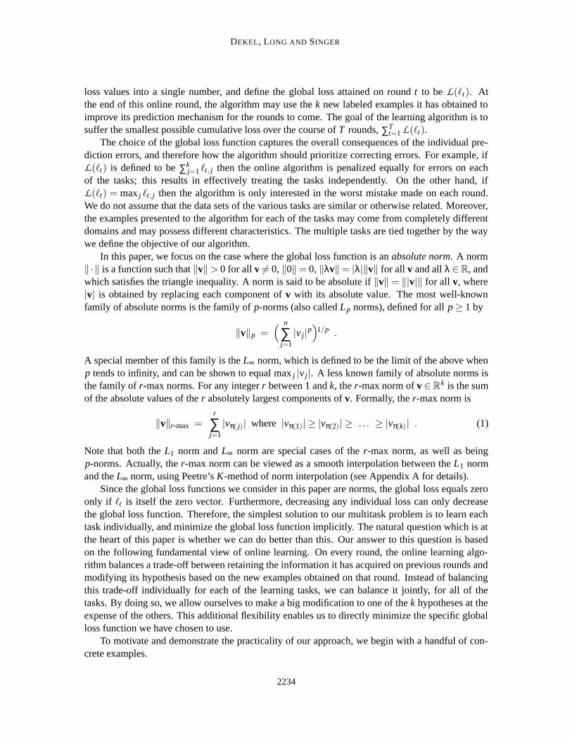
In this paper, we present three families of online multitask algorithms. Each family includesalgorithms for every absolute norm. All of the algorithms presented in this paper follow the gen-eral skeleton outlined in Figure 1. Specifically, all of our algorithms use linear threshold functionsas hypotheses and an additive update rule. The first two families are multitask extensions of thePerceptron algorithm (Rosenblatt, 1958; Novikoff, 1962), while the third family is closely relatedto the Passive-Aggressive classification algorithm (Crammer et al., 2006). Incidentally, all of thealgorithms presented in this paper can be easily transformed into kernel methods. For each algo-rithm, we prove a relative loss bound, namely, we show that the cumulative global loss attained bythe algorithm is comparable to the cumulative loss attained by any fixed set of k linear hypotheses,even defined in hindsight.

Much previous work on theoretical and applied multitask learning has focused on how to takeadvantage of similarities between the various tasks (Caruana, 1997; Heskes, 1998; Evgeniou et al.,2005; Baxter, 2000; Ben-David and Schuller, 2003; Tsochantaridis et al., 2004); in contrast, wedo not assume that the tasks are in any way related. Instead, we consider how to take account ofshared consequences of errors. Kivinen and Warmuth (2001) generalized the notion of matchingloss (Helmbold et al., 1999) to multi-dimensional outputs. Their construction enables analysis ofalgorithms that perform multi-dimensional regression by composing linear functions with a varietyof transfer functions. It is not obvious how to directly use their work to address the problems thatfall into our setting. An analysis of the L∞ norm of prediction errors is implicit in some past work ofCrammer and Singer (2001, 2003). The algorithms presented in Crammer and Singer (2001, 2003)were devised for multiclass categorization with multiple predictors (one per class) and a singleinstance. The present paper extends the multiclass prediction setting to a broader framework, andtightens the analysis. In contrast to the multiclass prediction setting, the prediction tasks in oursetting are tied solely through a globally shared loss. When k, the number of multiple tasks, is setto 1, two of the algorithms presented in this paper as well as the multiclass algorithms in Crammerand Singer (2001, 2003) reduce to the PA-I algorithm, presented in Crammer et al. (2006). Last, wewould like to mention in passing that a few learning algorithms for ranking problems decompose theranking problem into a preference learning task over pairs of instances (see for instance Herbrichet al., 2000; Chapelle and Harchaoui, 2005). The ranking losses employed by such algorithms aretypically defined as the sum over pair-based losses. Our setting generalizes such approaches forranking learning by employing a shared loss which is defined through a norm over the individualpair-based losses.

This paper is organized as follows. In Section 2 we present our problem more formally andprove a key lemma which facilitates the analysis of our algorithms. In Section 3 we present ourfirst family of algorithms, which works in the finite-horizon online setting. In Section 4 we extendthe first family of algorithms to the infinite-horizon online setting. Then, in Section 5 we presentour third family of algorithms, and show that it shares the analyses of both previous families. Thethird family of algorithms requires solving a small optimization problem on each online round, andis therefore called the implicit update family of algorithms. In Section 6 and Section 7 we describe

2236


input: norm ‖ · ‖initialize: w1,1 = . . . = w1,k = (0, . . . ,0)

for t = 1,2, . . .

• receive xt,1, . . . ,xt,k

• predict sign(wt, j ·xt, j) [1 ≤ j ≤ k]

• receive yt,1, . . . ,yt,k

• calculate `t, j =[1− yt, jwt, j ·xt, j

]

+[1 ≤ j ≤ k]

• suffer loss `t = ‖(`t,1, . . . , `t,n)‖• update wt+1, j = wt, j + τt, jyt, jxt, j [1 ≤ j ≤ k]

Figure 1: A general skeleton for an online multitask classification algorithm. A concrete algorithmis obtained by specifying the values of τt, j.

efficient algorithms for solving the implicit update in the case where the global loss is defined bythe L2 norm or the r-max norm. Experimental results are provided in Section 8 and we conclude thepaper in Section 9 with a short discussion.

2. Online Multitask Learning with Additive Updates

We begin by presenting the online multitask classification setting more formally. We are presentedwith k online binary classification problems in parallel. The instances of each task are drawn fromseparate instance domains, and for concreteness we assume that the instances of task j are all vectorsin R

n j . As stated in the previous section, online learning is performed in a sequence of rounds.On round t, the algorithm observes k instances, (xt,1, . . . ,xt,k) ∈ R

n1 × . . .×Rnk . The algorithm

maintains k separate classifiers in its internal memory, one for each of the multiple tasks, which areupdated from round to round. Each of these classifiers is a margin-based linear predictor, definedby a weight vector. We denote the weight vector used on round t to define the j’th predictor by wt, j

and note that wt, j ∈Rn j . The algorithm uses its classifiers to make k binary predictions, yt,1, . . . , yt,k,

where yt, j = sign(wt, j · xt, j). After making these predictions, the correct labels of the respectivetasks, yt,1, . . . ,yt,k, are revealed and each one of the predictions is evaluated. In this paper we focuson the hinge-loss function as the means of penalizing incorrect predictions. Formally, the lossassociated with the j’th task is defined to be

`t, j =[1− yt, jwt, j ·xt, j

]

+,

where [a]+ = max{0,a}. As previously stated, the global loss is then defined to be ‖`t‖, where‖ · ‖ is a predefined absolute norm. Finally, the algorithm applies an update to each of the onlinehypotheses, and defines the vectors wt+1,1, . . . ,wt+1,k. All of the algorithms presented in this paperuse an additive update rule, and define wt+1, j to be wt, j + τt, jyt, jxt, j, where τt, j is a scalar. Thealgorithms only differ from one another in the specific way in which τt, j is set. For convenience, we

2237


denote τt = (τt,1, . . . ,τt,k). The general skeleton followed by all of our online algorithms is given inFigure 1.

A concept of key importance in this paper is the notion of dual norms (Horn and Johnson, 1985).Any norm ‖ · ‖ defined on R

n, has a dual norm, also defined on Rn, denoted by ‖ · ‖∗ and given by

‖u‖∗ = maxv∈Rn

u ·v‖v‖ = max

v∈Rn :‖v‖=1u ·v . (2)

The dual of a p-norm is itself a p-norm, and specifically, the dual of ‖ ·‖p is ‖ ·‖q, where 1q + 1

p = 1.The dual of ‖ · ‖∞ is ‖ · ‖1 and vice versa. In Appendix A we prove that the dual of ‖v‖r-max is

‖u‖∗r-max = max

{

‖u‖∞,‖u‖1

r

}

. (3)

An important property of dual norms, which is an immediate consequence of Equation (2), is thatfor any u,v ∈ R

n it holds thatu ·v ≤ ‖u‖∗ ‖v‖ . (4)

If ‖ · ‖ is a p-norm then the above is known as Holder’s inequality, and specifically, if p = 2 it iscalled the Cauchy-Schwartz inequality. Two additional properties which we rely on are that the dualof the dual norm is the original norm (see for instance Horn and Johnson, 1985), and that the dualof an absolute norm is also an absolute norm. As previously mentioned, to obtain concrete onlinealgorithms, all that remains is to define the update weights τt, j for each task on each round. Thedifferent ways of setting τt, j discussed in this paper all share the following properties:

• boundedness: ∀ 1 ≤ t ≤ T ‖τt‖∗ ≤C for some predefined parameter C

• non-negativity: ∀ 1 ≤ t ≤ T, 1 ≤ j ≤ k τt, j ≥ 0

• conservativeness: ∀ 1 ≤ t ≤ T, 1 ≤ j ≤ k (`t, j = 0) ⇒ (τt, j = 0)

Even before specifying the exact value of τt, j, we can state and prove a powerful lemma which isthe crux of our analysis. This lemma will motivate and justify our specific choices of τt, j throughoutthis paper.

Lemma 1 Let {(xt, j,yt, j)}1≤ j≤k1≤t≤T be a sequence of T k-tuples of examples, where each xt, j ∈ R

n j ,and each yt, j ∈ {−1,+1}. Let w?

1, . . . ,w?k be arbitrary vectors where w?

j ∈ Rn j , and define the hinge

loss attained by w?j on example (xt, j,yt, j) to be `?

t, j =[1− yt, jw?

j · xt, j]

+. Let ‖ · ‖ be an arbitrary

norm and let ‖ · ‖∗ denote its dual. Assume we apply an algorithm of the form outlined in Figure 1to this sequence of examples, where the update weights satisfy the boundedness, non-negativity andconservativeness requirements. Then, for any C > 0 it holds that

T

∑t=1

k

∑j=1

(

2τt, j`t, j − τ2t, j‖xt, j‖2

2

)

≤k

∑j=1

‖w?j‖2

2 + 2CT

∑t=1

‖`?t‖ .

Under the assumptions of this lemma, our algorithm competes with a set of fixed linear classifiers,w?

1, . . . ,w?k , which may even be defined in hindsight, after observing all of the inputs and their labels.

The right-hand side of the bound is the sum of two terms, a complexity term ∑kj=1 ‖w?

j‖22 and a term

2238


which is proportional to the cumulative loss of our competitor, ∑Tt=1 ‖`?

t‖. The left hand side of thebound is the term

T

∑t=1

k

∑j=1

(

2τt, j`t, j − τ2t, j‖xt, j‖2

2

)

. (5)

This term plays a key role in the derivation of all three families of algorithms presented in the sequel.Each choice of the update weights τt, j enables us to prove a different lower bound on Equation (5).Comparing this lower bound with the upper bound in Lemma 1 gives us a loss bound for the respec-tive algorithm. The proof of Lemma 1 is given below.

Proof Define ∆t, j = ‖wt, j−w?j‖2

2−‖wt+1, j−w?j‖2

2. We prove the lemma by bounding ∑Tt=1 ∑k

j=1 ∆t, j

from above and from below. Beginning with the upper bound, we note that for each 1 ≤ j ≤ k,∑T

t=1 ∆t, j is a telescopic sum which collapses to

T

∑t=1

∆t, j = ‖w1, j −w?‖22 −‖wT+1, j −w?‖2

2 .

Using the facts that w1, j = (0, . . . ,0) and ‖wT+1, j −w?‖22 ≥ 0 for all 1 ≤ j ≤ k, we conclude that

T

∑t=1

k

∑j=1

∆t, j ≤k

∑j=1

‖w?j‖2

2 . (6)

Turning to the lower bound, we note that we can consider only non-zero summands which actuallycontribute to the sum, namely ∆t, j 6= 0. Plugging the definition of wt+1, j into ∆t, j, we get

∆t, j = ‖wt, j −w?j‖2

2 −‖wt, j + τt, jyt, jxt, j −w?j‖2

2

= τt, j(−2yt, jwt, j ·xt, j − τt, j‖xt, j‖2

2 +2yt, jw?j ·xt, j

)

= τt, j(2(1− yt, jwt, j ·xt, j)− τt, j‖xt, j‖2

2 −2(1− yt, jw?j ·xt, j)

). (7)

Since our update is conservative, ∆t, j 6= 0 implies that `t, j = 1− yt, jwt, j ·xt, j. By definition, it alsoholds that `?

t, j ≥ 1− yt, jw?j · xt, j. Plugging these two facts into Equation (7) and using the fact that

τt, j is non-negative gives

∆t, j ≥ τt, j(2`t, j − τt, j‖xt, j‖2

2 −2`?t, j

).

Summing the above over 1 ≤ j ≤ k gives

k

∑j=1

∆t, j ≥k

∑j=1

(2τt, j`t, j − τ2

t, j‖xt, j‖22

)−2

k

∑j=1

τt, j`?t, j . (8)

Using Equation (4) we know that ∑kj=1 τt, j`

?t, j ≤ ‖τt‖∗‖`?

t‖. From our assumption that ‖τt‖∗ ≤C, we

have that ∑kj=1 τt, j`

?t, j ≤C‖`?

t‖. Plugging this inequality into Equation (8) gives

k

∑j=1

∆t, j ≥k

∑j=1

(2τt, j`t, j − τ2

t, j‖xt, j‖22

)−2C‖`?

t‖ .

We conclude the proof by summing the above over 1 ≤ t ≤ T and comparing the result to the upperbound in Equation (6).

2239


3. The Finite-Horizon Multitask Perceptron

In this section, we present our first family of online multitask classification algorithms, and prove arelative loss bound for the members of this family. This family includes algorithms for any globalloss function defined through an absolute norm. These algorithms are finite-horizon online algo-rithms, meaning that the number of online rounds, T , is known in advance and is given as a param-eter to the algorithm. An analogous family of infinite-horizon algorithms is the topic of the nextsection.

As previously noted, the Finite-Horizon Multitask Perceptron follows the general skeleton out-lined in Figure 1. Given an absolute norm ‖ · ‖ and its dual ‖ · ‖∗, the multitask Perceptron sets τt, j

in Figure 1 toτt = argmax

τ:‖τ‖∗≤Cτ· `t , (9)

where C > 0 is a constant which is specified later in this section. There may exist multiple solutionsto the maximization problem above and at least one of these solutions induces a conservative update.In other words, we may assume that the solution to Equation (9) is such that τt, j = 0 at everycoordinate j where `t, j = 0. To see that such a solution exists, take an arbitrary optimal solution τand let τ be defined by

τ j =

{τ j if `t, j 6= 00 if `t, j = 0.

Clearly, τ· `t = τ· `t , whereas ‖τ‖∗ ≤ ‖τ‖∗ ≤ C. If the optimization problem in Equation (9) hasmultiple solutions that induce conservative updates, assume that one is chosen arbitrarily.

An equivalent way of defining the solution to Equation (9) is by satisfying the equality τt · `t =C‖`t‖. To see this equivalence, note that the dual of ‖ · ‖∗ is defined by Equation (2) to be

‖`‖∗∗ = maxτ:‖τ‖∗≤1

τ· ` .

However, since ‖ · ‖∗∗ is equivalent to ‖ · ‖ (see for instance Theorem 5.5.14 in Horn and Johnson,1985), we get

‖`‖ = maxτ:‖τ‖∗≤1

τ· ` .

Using the linearity of ‖ · ‖∗, we conclude that ‖τ/C‖∗ = ‖τ‖∗/C for any C > 0, and therefore theabove becomes

C‖`‖ = maxτ:‖τ‖∗≤C

τ· ` .

We conclude thatτt · `t = C‖`t‖ (10)

holds if and only if τt is a maximizer of Equation (9).When the global loss function is a p-norm, the following definition of τt solves Equation (9):

τt, j =C` p−1

t, j

‖`t‖p−1p

. (11)

When the global loss function is an r-max norm and π is a permutation such that `t,π(1) ≥ . . .≥ `t,π(k),the following definition of τt is a solution to Equation (9):

τt, j =

{C if `t, j > 0 and j ∈ {π(1), . . . ,π(r)}0 otherwise.

(12)

2240


1 16√

2√

2

L1 norm L2 norm L3 norm L∞ norm

Figure 2: The remoteness of a norm is the longest Euclidean length of any vector contained in thenorm’s unit ball. The longest vector in each of the two-dimensional unit balls above isdepicted with an arrow.

Note that when r = k, the r-max norm reduces to the L1 norm and the above becomes the well-knownupdate rule of the Perceptron algorithm (Rosenblatt, 1958; Novikoff, 1962). The correctness of thedefinitions in Equation (11) and Equation (12) can be easily verified by observing that ‖τt‖∗ ≤ Cand that τt · `t = C‖`t‖ in both cases.

Before proving a loss bound for the multitask Perceptron, we must introduce another importantquantity. This quantity is the remoteness of a norm ‖ · ‖ defined on R

k, and is defined to be

ρ(‖ · ‖,k) = maxu∈Rk

‖u‖2

‖u‖ = maxu∈Rk:‖u‖≤1

‖u‖2 . (13)

Geometrically, the remoteness of ‖ ·‖ is simply the Euclidean length of the longest vector (again, inthe Euclidean sense) which is contained in the unit ball of ‖ · ‖. This definition is visually depictedin Figure 2. As we show below, the remoteness of the dual norm, ρ(‖ · ‖∗,k), plays an importantrole in determining the difficulty of using ‖ · ‖ as the global loss function.

For concreteness, we now calculate the remoteness of the duals of p-norms and of r-max norms.

Lemma 2 The remoteness of a p-norm ‖ · ‖q equals

ρ(‖ · ‖q,k) =

{

1 if 1 ≤ q ≤ 2

k( 12− 1

q ) if 2 < q.

Before proving the lemma, we note that if ‖ · ‖p is a p-norm and ‖ · ‖q is its dual, then we cancombine Lemma 2 with the equality q = p

p−1 to obtain

ρ(‖ · ‖q,k) =

{

1 if 2 ≤ p

k( 1p− 1

2 ) if 1 ≤ p < 2.

This equivalent form is better suited to our needs. The proof of Lemma 2 is given below.

Proof If 2 ≤ p then 1 ≤ q ≤ 2, and the monotonicity of the p-norms implies that ‖v‖q ≥ ‖v‖2 forall v ∈ R

k. Therefore ‖v‖2/‖v‖q ≤ 1 for all v ∈ Rk and thus ρ(‖ · ‖q,k) ≤ 1. On the other hand,

2241


setting v = (1,0, . . . ,0), we get ‖v‖q = ‖v‖2 and therefore ρ(‖ · ‖q,k) ≥ 1. Overall, we have shownthat ρ(‖ · ‖q,k) = 1.

Turning to the case where 1 ≤ p < 2, we note that q > 2. Let v be an arbitrary vector in Rk,

and define u = (v21, . . . ,v

2k) and w = (1, . . . ,1). Noting that ‖ ·‖ q

2and ‖ ·‖ q

q−2are dual norms, we use

Holder’s inequality to obtainu ·w ≤ ‖u‖ q

2‖w‖ q

q−2.

The left-hand side above equals ‖v‖22, while the right-hand side above equals ‖v‖2

q k1− 2q . There-

fore, ‖v‖22/‖v‖2

q ≤ k1− 2q and taking square-roots on both sides yields ‖v‖2/‖v‖q ≤ k

12− 1

q . Since

this inequality holds for all v ∈ Rk, we have shown that ρ(‖ · ‖q,k) ≤ k

12− 1

q . On the other hand,

setting v = (1, . . . ,1), we get ‖v‖2 = k12− 1

q ‖v‖q. This proves that ρ(‖ · ‖q,k) ≥ k12− 1

q , and therefore

ρ(‖ · ‖q,k) = k12− 1

q .

Lemma 3 Let ‖ · ‖r-max be a r-max norm and let ‖ · ‖∗r-max be its dual. The remoteness of ‖ · ‖∗r-maxequals

√r.

Proof Using Equation (13), the remoteness of ‖ ·‖∗r-max is defined to be the maximum value of ‖u‖2

subject to ‖u‖∗r-max ≤ 1. Recalling the definition of ‖ · ‖∗r-max from Equation (3), we can replacethis constraint with two constraints ‖u‖1 ≤ r and ‖u‖∞ ≤ 1. Moreover, since both the L1 norm andthe L∞ norm are absolute norms, we can also assume that u resides in the non-negative orthant.Therefore, we have that 0 ≤ u j ≤ 1 for all 1 ≤ j ≤ k. From this we conclude that u2

j ≤ u j for all1 ≤ j ≤ k, and thus ‖u‖2

2 ≤ ‖u‖1 ≤ r. Hence, ‖u‖2 ≤√

r and ρ(‖ · ‖∗r-max,k) ≤√

r. On the otherhand, the vector

u =(

r︷︸︸︷

1, . . . ,1,

k−r︷︸︸︷

0, . . . ,0)

is contained in the unit ball of ‖ ·‖∗r-max, and its Euclidean length is√

r. Therefore, we also have thatρ(‖ · ‖∗r-max,k) ≥

√r, and overall we get ρ(‖ · ‖∗r-max,k) =

√r.

We are now ready to prove a loss bound for the Finite-Horizon Multitask Perceptron.

Theorem 4 Let {(xt, j,yt, j)}1≤ j≤k1≤t≤T be a sequence of T k-tuples of examples, where each xt, j ∈ R

n j ,‖xt, j‖2 ≤ R and each yt, j ∈ {−1,+1}. Let C be a positive constant and let ‖·‖ be an absolute norm.Let w?


j ∈ Rn j , and define the hinge loss incurred by w?

j onexample (xt, j,yt, j) to be `?

t, j =[1− yt, jw?

j · xt, j]

+. If we present this sequence to the finite-horizon

multitask Perceptron with the norm ‖ · ‖ and the aggressiveness parameter C, then,

T

∑t=1

‖`t‖ ≤ 12C

k

∑j=1

‖w?j‖2

2 +T

∑t=1

‖`?t‖ +

T R2C ρ2(‖ · ‖∗,k)2

.

Proof The starting point of our analysis is Lemma 1. The choice of τt, j in Equation (9) is clearlybounded by ‖τt‖∗ ≤C and conservative. It is also non-negative, due to the fact that ‖ · ‖∗ is an abso-lute norm and that `t, j ≥ 0. Therefore, the definition of τt, j in Equation (9) meets the requirements

2242


of the lemma, and we have

T

∑t=1

k

∑j=1

(

2τt, j`t, j − τ2t, j‖xt, j‖2

2

)

≤k

∑j=1

‖w?j‖2

2 + 2CT

∑t=1

‖`?t‖ .

Using Equation (10), we rewrite the left-hand side of the above as

2CT

∑t=1

‖`t‖−T

∑t=1

k

∑j=1

τ2t, j‖xt, j‖2

2 . (14)

Using our assumption that ‖xt, j‖22 ≤ R2, we know that ∑k

j=1 τ2t, j‖xt, j‖2

2 ≤ (R‖τt‖2)2. Using the

definition of remoteness, we can upper bound this term by (R‖τt‖∗ρ(‖ · ‖∗,k))2. Finally, using ourupper bound on ‖τt‖∗ we can further bound this term by R2C2ρ2(‖ ·‖∗,k). Plugging this bound backinto Equation (14) gives

2CT

∑t=1

‖`t‖ − T R2C2ρ2(‖ · ‖∗,k) .

Overall, we have shown that

2CT

∑t=1

‖`t‖ − T R2C2ρ2(‖ · ‖∗,k) ≤k

∑j=1

‖w?j‖2

2 + 2CT

∑t=1

‖`?t‖ .

Dividing both sides of the above by 2C and rearranging terms gives the desired bound.

In its current form, the bound in Theorem 4 may seem insignificant, since its right-most term growslinearly with the length of the input sequence, T . This term can be easily controlled by setting C toa value on the order of 1/

√T .

Corollary 5 Under the assumptions of Theorem 4, if C = 1/(√

T R2), then

T

∑t=1

‖`t‖ ≤T

∑t=1

‖`?t‖ +

√T

2

(

R2k

∑j=1

‖w?j‖2

2 + ρ2(‖ · ‖∗,k))

.

This corollary bounds the global loss cumulated by our algorithm with the global loss obtained byany fixed set of hypotheses, plus a term which grows sub-linearly in T . The significance of this termdepends on the magnitude of the constant

12

(

R2k

∑j=1

‖w?j‖2

2 + ρ2(‖ · ‖∗,k))

.

Our algorithm uses C in its update procedure, and the value of C depends on√

T . Therefore, thealgorithm is a finite horizon algorithm.

Dividing both sides of the inequality in Corollary 5 by T , we see that the average global losssuffered by the multitask Perceptron is upper bounded by the average global loss of the best fixedhypothesis ensemble plus a term that diminishes with T . Using game-theoretic terminology, we cannow say that the multitask Perceptron exhibits no-regret with respect to any global loss functiondefined by an absolute norm. The same cannot be said for the naive alternative of learning each

2243


task independently using a separate single-task Perceptron. We show this by presenting a simplecounter-example. Specifically, we construct a concrete k-task problem with a specific global loss,an arbitrarily long input sequence {(xt, j,yt, j)}1≤ j≤k

1≤t≤T , and fixed weight vectors u1, . . . ,uk to use forcomparison. We then prove that

k +12

T

∑t=1

‖`?t‖∞ ≤

T

∑t=1

‖ ˆt‖∞ , (15)

where ˆt is the vector of individual losses of the k independent single-task Perceptrons, and, asbefore, `?

t is the vector of individual losses of u1, . . . ,uk respectively. This example demonstratesthat a claim along the lines of Corollary 5 cannot be proven for the set of independent single-taskPerceptrons.

First, we would like to emphasize that we are considering a version of the single-task Perceptronthat updates its hypothesis whenever it suffers a positive hinge-loss, and not only when it makes aprediction mistake. Moreover, when an update is performed, the algorithm defines wt+1 = wt +Cytxt , where C is a predefined constant. This version of the Perceptron is sometimes called theaggressive Perceptron. If we were to use the simplest version of the Perceptron, which updatesits hypothesis only when a prediction mistake occurs, then finding a counter-example that achievesEquation (15) would be trivial, without even using the distinction between single-task and multitaskPerceptron learning.

Also, we can assume without loss of generality that 1/C = o(T ), since otherwise, even in thecase k = 1, simply repeating the same example over and over provides a counterexample.

Moving on to the counter-example itself, assume that our global loss is defined by the L∞ norm.Let k be at least 2, assume that the instances of all k problems are two dimensional vectors, andset u1 = . . . = uk = (1,1). Each of the single-task Perceptrons initializes its hypothesis to (0,0).Assume that all of the labels in the input sequence are positive labels. For t = 0, we set x1,1 = . . . =x1,k = (1,0). Each one of the independent Perceptrons suffers a positive individual loss and updatesits weight vector to (C,0). We continue presenting the same example for d1/Ce − 1 additionalrounds, which is precisely when all k weight vectors of the Perceptrons become equal to (α,0), withα ≥ 1. For instance, if C = O(1/

√T ) then the vector (1,0) is presented O(

√T ) times. Meanwhile,

the fixed weight vectors u1, . . . ,uk suffer no loss at all.Define t0 = d1/Ce, and note that the index of the next online round is t0 + 1. For each t in

t0 +1, . . . , t0 + k, we set xt,t−t0 to (0,1) and xt, j to (1,0) for all j 6= t − t0. On round t, the (t − t0)’thPerceptron, whose weight vector is (α,0), suffers an individual loss of 1 and updates its weightvector to (α,C). The remaining k−1 Perceptrons suffer no individual loss and do not modify theirweight vectors. Consequently, ‖ ˆt‖∞ = 1 on each of these rounds. Once again, the fixed vectorsu1, . . . ,uk suffer no loss at all. On round t = t0 +k+1, we set xt,1 = . . . = xt,k = (0,−1). As a result,each of the Perceptrons suffers a hinge loss of 1 +C and updates its weight vector back to (α,0).Since C is positive, we get ‖ ˆt‖∞ ≥ 1. Meanwhile, ‖`?

t‖∞ = 2. We now have that

t0+k+1

∑t=t0+1

‖ ˆt‖∞ ≥ k +1 andt0+k+1

∑t=t0+1

‖`?t‖∞ = 2 .

Furthermore, the weight vectors of the k single-task Perceptrons have returned to their values at theend of round t0. Therefore, by repeating the input sequence from round t0 + 1 to round t0 + k + 1over and over again, we obtain Equation (15).

2244


This concludes the presentation of the counter-example thus showing that a set of independentsingle-task Perceptrons does not attain no-regret with respect to the L∞ norm global loss. Similarconstructions can be given for other global loss functions. The exception is the L1 norm, whichnaturally reduces the multitask Perceptron to k independent single-task Perceptrons.

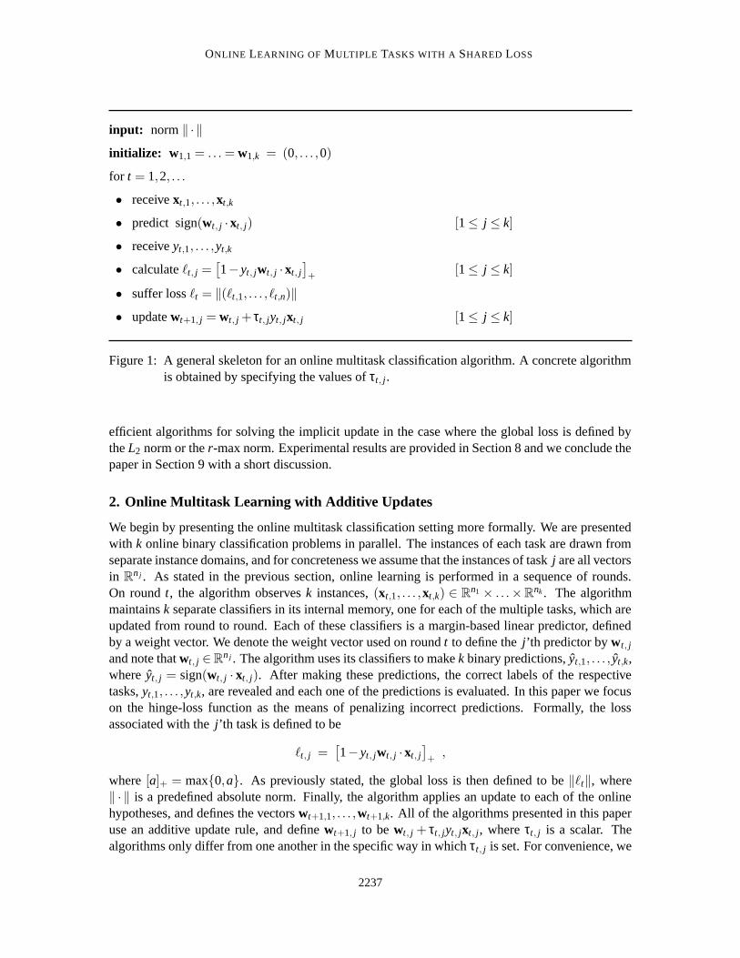
4. An Extension to the Infinite Horizon Setting

In the previous section, we devised an algorithm which relied on prior knowledge of T , the inputsequence length. In this section, we adapt the update procedure from the previous section to theinfinite horizon setting, where T is not known in advance. Moreover, the bound we prove in thissection holds simultaneously for every prefix of the input sequence. This generalization comes ata price; we can only prove an upper bound on ∑t min{`t , `

2t }, a quantity similar to the cumulative

global loss, but not the global loss per se.To motivate our infinite-horizon algorithm, we take a closer look at the analysis of the finite-

horizon algorithm. In the proof of Theorem 4, we lower-bounded the term ∑kj=1 2τt, j`t, j −τ2

t, j‖xt, j‖22

by 2C‖`t‖−R2C2ρ2(‖ · ‖∗,k). The first term in this lower bound is proportional to the global losssuffered on round t, and the second term is a constant. When ‖`t‖ is smaller than this constant, ourlower bound becomes negative. This suggests that the update step-size applied by the finite-horizonPerceptron may have been too large, and that the update step may have overshot its target. As aresult, the new hypothesis may be inferior to the previous one. Nevertheless, over the course of Trounds, our positive progress is guaranteed to overshadow our negative progress, and thus we areable to prove Theorem 4. However, if we are interested in a bound which holds for every prefix of theinput sequence, we must ensure that every individual update makes positive progress. Concretely,we derive an update for which ∑k

j=1 2τt, j`t, j − τ2t, j‖xt, j‖2

2 is guaranteed to be non-negative. Thevector τt remains in the same direction as before, but by setting its length more carefully, we enforcean update step-size which is never excessively large.

We use ρ to abbreviate ρ(‖ · ‖∗,k) throughout this section. We replace the definition of τt inEquation (9) with the following definition,

τt = argmaxτ:‖τ‖∗≤min

{

C, ‖`t ‖R2ρ2

}τ· `t , (16)

where C > 0 is a user defined parameter and R > 0 is an upper bound on ‖xt, j‖2 for all 1 ≤ t ≤ Tand all 1 ≤ j ≤ k. As in the previous section, we assume that τt, j = 0 whenever `t, j = 0. As inEquation (10), the solution to Equation (16) can be equivalently defined by the equation

τt · `t = min

{

C,‖`t‖R2ρ2

}

‖`t‖ . (17)

When the global loss function is a p-norm, the following definition of τt solves Equation (16):

τt, j =

`p−1t, j

R2ρ2‖`t‖p−2p

if ‖`t‖p ≤ R2Cρ2

C`p−1t, j

‖`t‖p−1p

if ‖`t‖p > R2Cρ2.

2245


When the global loss function is an r-max norm and π is a permutation such that `t,π(1) ≥ . . .≥ `t,π(k),then the following definition of τt is a solution to Equation (16):

τt, j =

‖`t‖r-max

rR2 if `t, j > 0 and ‖`t‖r-max ≤ R2Cρ2 and j ∈ {π(1), . . . ,π(r)}

C if `t, j > 0 and ‖`t‖r-max > R2Cρ2 and j ∈ {π(1), . . . ,π(r)}

0 otherwise.

The correctness of both definitions of τt, j given above can be verified by observing that ‖τt‖∗ ≤min{C, ‖`t‖

R2ρ2 } and that τt · `t = min{C, ‖`t‖R2ρ2 }‖`t‖ in both cases. We now turn to proving an infinite-

horizon cumulative loss bound for our algorithm.

Theorem 6 Let {(xt, j,yt, j)}1≤ j≤kt=1,2,... be a sequence of k-tuples of examples, where each xt, j ∈ R

n j ,‖xt, j‖2 ≤ R and each yt, j ∈ {−1,+1}. Let C be a positive constant, let ‖ · ‖ be an absolute norm,and let ρ be an abbreviation for ρ(‖ · ‖∗,k). Let w?


j ∈ Rn j ,

and define the hinge loss attained by w?j on example (xt, j,yt, j) to be `?

t, j =[1− yt, jw?

j ·xt, j]

+. If we

present this sequence to the explicit multitask algorithm with the norm ‖ · ‖ and the aggressivenessparameter C, then for every T

1/(R2ρ2) ∑t≤T :‖`t‖≤R2Cρ2

‖`t‖2 + C ∑t≤T :‖`t‖>R2Cρ2

‖`t‖ ≤ 2CT

∑t=1

‖`?t‖ +

k

∑j=1

‖w?j‖2

2 .

Proof The starting point of our analysis is again Lemma 1. The choice of τt, j in Equation (16) isclearly bounded by ‖τt‖∗ ≤ C and conservative. It is also non-negative, due to the fact that ‖ · ‖∗ isabsolute and that `t, j ≥ 0. Therefore, τt, j meets the requirements of Lemma 1, and we have

T

∑t=1

k

∑j=1

(

2τt, j`t, j − τ2t, j‖xt, j‖2

2

)

≤k

∑j=1

‖w?j‖2

2 + 2CT

∑t=1

‖`?t‖ . (18)

We now prove our theorem by lower-bounding the left hand side of Equation (18) above. We analyzetwo different cases. First, if ‖`t‖ ≤ R2Cρ2 then min{C,‖`t‖/(R2ρ2)}= ‖`t‖/(R2ρ2). Together withEquation (17), this gives

2k

∑j=1

τt, j`t, j = 2‖τt‖∗ ‖`t‖ = 2‖`t‖2

R2ρ2 . (19)

On the other hand, ∑kj=1 τ2

t, j‖xt, j‖22 can be bounded by ‖τt‖2

2R2. Using the definition of remoteness,we bound this term by (‖τt‖∗)2R2ρ2. Using the fact that, ‖τt‖∗ ≤ ‖`t‖/(R2ρ2), we bound this termby ‖`t‖2/(R2ρ2). Overall, we have shown that

k

∑j=1

τ2t, j‖xt, j‖2

2 ≤ ‖`t‖2

R2ρ2 .

Subtracting both sides of the above inequality from the respective sides of Equation (19) gives

‖`t‖2

R2ρ2 ≤k

∑j=1

(2τt, j`t, j − τ2

t, j‖xt, j‖22

). (20)

2246


Moving on to the second case, if ‖`t‖> R2Cρ2 then min{C,‖`t‖/(R2ρ2)}=C. Using Equation (17),we have that

2k

∑j=1

τt, j`t, j = 2‖τt‖∗ ‖`t‖ = 2C‖`t‖ . (21)

As before, we can upper bound ∑kj=1 τ2

t, j‖xt, j‖22 by (‖τt‖∗)2R2ρ2. Using the fact that, ‖τt‖∗ ≤C we

can bound this term by C2R2ρ2. Finally, using our assumption that ‖`t‖ > R2Cρ2, we conclude that

k

∑j=1

τ2t, j‖xt, j‖2

2 < C‖`t‖ .

Subtracting both sides of the above inequality from the respective sides of Equation (21) gives

C‖`t‖ ≤k

∑j=1

(2τt, j`t, j − τ2

t, j‖xt, j‖22

). (22)

Comparing the upper bound in Equation (18) with the lower bounds in Equation (20) and Equa-tion (22) proves the theorem.

Corollary 7 Under the assumptions of Theorem 6, if C is set to be 1/(R2ρ2) then for every T ′ ≤ Tit holds that,

T ′

∑t=1

min{‖`t‖2,‖`t‖

}≤ 2

T ′

∑t=1

‖`?t‖ + R2ρ2

k

∑j=1

‖w?j‖2

2 .

As noted at the beginning of this section, we do not obtain a cumulative loss bound per se, but ratherat a bound on ∑t min{`t , `

2t }. However, this bound holds simultaneously for every prefix of the input

sequence, and the algorithm does not rely on knowledge of the input sequence length.

5. The Implicit Online Multitask Update

We now discuss a third family of online multitask algorithms, which leads to the strongest lossbounds of the three families of algorithms presented in this paper. In contrast to the closed formupdates of the previous algorithms, the algorithms in this family require solving an optimizationproblem on every round, and are therefore called implicit update algorithms. Although the imple-mentation of specific members of this family may be more involved than the implementation of themultitask Perceptron, we recommend using this family of algorithms in practice. On every round,the set of hypotheses is updated according to the update rule:

{wt+1,1, . . . ,wt+1,k} = argminw1,...,wk

12

k

∑j=1

‖w j −wt, j‖22 +C‖ξ‖ (23)

s.t. ∀ j w j ·xt, j ≥ 1−ξ j and ξ j ≥ 0.

This optimization problem captures the fundamental tradeoff inherent to online learning. On onehand, the term ∑k

j=1 ‖w j −wt, j‖22 in the objective function above keeps the new set of hypotheses

close to the current set of hypotheses, so as to retain the information learned on previous rounds. On

2247


input: aggressiveness parameter C > 0, norm ‖ · ‖initialize w1,1 = . . . = w1,k = (0, . . . ,0)

for t = 1,2, . . .

• receive xt,1, . . . ,xt,k

• predict sign(wt, j ·xt, j) [1 ≤ j ≤ k]

• receive yt,1, . . . ,yt,k

• suffer loss `t, j =[1− yt, jwt, j ·xt, j

]

+[1 ≤ j ≤ k]

• update:

{wt+1,1, . . . ,wt+1,k} = argminw1,...,wk

12 ∑k

j=1 ‖w j −wt, j‖22 +C‖ξ‖

s.t. ∀ j w j ·xt, j ≥ 1−ξ j and ξ j ≥ 0

Figure 3: The implicit update algorithm

the other hand, the term ‖ξ‖ in the objective function, together with the constraints on ξ j, forces thealgorithm to make progress using the new examples obtained on this round. Different choices of theglobal loss function lead to different definitions of this progress. The pseudo-code of the implicitupdate algorithm is presented in Figure 3.

Our first task is to show that this update procedure follows the skeleton outlined in Figure 1, andsatisfies the requirements of Lemma 1. We do so by finding the dual of the optimization problemgiven in Equation (23).

Lemma 8 Let ‖ · ‖ be a norm and let ‖ · ‖∗ be its dual. Then the online update defined in Equa-tion (23) is equivalent to setting wt+1, j = wt, j + τt, jyt, jxt, j for all 1 ≤ j ≤ k, where

τt = argmaxτ

k

∑j=1

(2τ j`t, j − τ2

j‖xt, j‖22

)

s.t. ‖τ‖∗ ≤C and ∀ j τ j ≥ 0 .

Moreover, this update is conservative.

Proof The update step in Equation (23) sets the vectors wt+1,1, . . . ,wt+1,k to be the solution to thefollowing constrained minimization problem:

minw1,...,wk,ξ≥0

12

k

∑j=1

‖w j −wt, j‖22 + C‖ξ‖

s.t. ∀ j yt, jw j ·xt, j ≥ 1−ξ j .

We begin by using the notion of strong duality to restate this optimization problem in an equivalentform. The objective function above is convex and the constraints are both linear and feasible, there-fore Slater’s condition (Boyd and Vandenberghe, 2004) holds, and the above problem is equivalent

2248


tomaxτ≥0

minw1,...,wk,ξ≥0

L(τ,w1, . . . ,wk,ξ) ,

where L(τ,w1, . . . ,wk,ξ) is defined as follows:

12

k

∑j=1

‖w j −wt, j‖22 +C‖ξ‖+

k

∑j=1

τ j (1− yt, jw j ·xt, j −ξ j) .

We can rewrite L as the sum of two terms, the first a function of τ and w1, . . . ,wk (denoted L1) andthe second a function of τ and ξ1, . . . ,ξk (denoted L2),

12

k

∑j=1

‖w j −wt, j‖22 +

k

∑j=1

τ j(1− yt, jw j ·xt, j)

︸︷︷︸

L1(τ,w1,...,wk)

+ C‖ξ‖−k

∑j=1

τ jξ j

︸︷︷︸

L2(τ,ξ)

.

Using the notation defined above, our optimization problem becomes,

maxτ≥0

(

minw1,...,wk

L1(τ,w1, . . . ,wk) + minξ≥0

L2(τ,ξ)

)

.

For any choice of τ, L1 is a convex function and we can find w1, . . . ,wk which minimize it by settingall of its partial derivatives with respect to the elements of w1, . . . ,wk to zero. Namely,

∀ j, l 0 =∂L1

∂w j,l= w j,l −wt, j,l − τ jyt, jxt, j,l .

from the above we conclude that w j = wt, j + τ jyt, jxt, j for all 1 ≤ j ≤ k.The next step is to show that the update is conservative. If `t, j = 0 then setting w j = wt, j satisfies

the constraint yt, jw j ·xt, j ≥ 1−ξ j with any choice of ξ j ≥ 0. Since choosing w j = wt, j minimizes‖wt −wt, j‖2

2 and does not restrict our choice of any other variable, then it is optimal. The relationbetween w j and τ j now implies that τ j = 0 whenever `t, j = 0).

Plugging our expression for w j into L1, we have that

minw1,...,wk

L1(τ,w1, . . . ,wk) =k

∑j=1

τ j(1− yt, jwt, j ·xt, j) − 12

k

∑j=1

τ2j‖xt, j‖ .

Since the update is conservative, it holds that τ j(1−yt, jwt, j ·xt, j) = τ j`t, j. Overall, we have reducedour optimization problem to

τt = argmaxτ≥0

(k

∑j=1

(

τ j`t, j −12

τ2j‖xt, j‖

)

+ minξ≥0

L2(τ,ξ)

)

.

We finally turn our attention to L2 and abbreviate B(τ) = minξ≥0 L2(τ,ξ). We now claim that B is abarrier function for the constraint ‖τ‖∗ ≤C, namely

B(τ) =

{0 if ‖τ‖∗ ≤C−∞ if ‖τ‖∗ > C

.

2249


To see why this is true, recall that ‖τ‖∗ is defined to be

‖τ‖∗ = maxε∈Rk

∑kj=1 τ jε j

‖ε‖ .

First, let us consider the case where ‖τ‖∗ > C. In this case there exists a vector ε for which

k

∑j=1

τ jε j −C‖ε‖ > 0 .

Denote the left hand side of the above by δ. We can assume w.l.o.g. that all the components of ε arenon-negative since τ≥ 0. For any c ≥ 0, we now have that

B(τ) = minξ≥0

L2(τ,ξ) ≤ L2(τ,cε) = − cδ .

Therefore, by taking c to infinity we get that B(τ) = −∞.Turning to the case ‖τ‖∗ ≤ C, we have that ∑k

j=1 τ jξ j ≤ C‖ξ‖ for any choice of ξ, or in otherwords, minξ≥0 L2(τ,ξ) ≥ 0. However, this lower bound is attainable by setting ξ = 0. We concludethat if ‖τ‖∗ ≤C then B(τ) = 0. The original optimization problem has reduced to the form

τt = argmaxτ≥0

(k

∑j=1

(

τ j`t, j −12

τ2j‖xt, j‖

)

+ B(τ)

)

.

Clearly, the above is maximized in the domain where B(τ) = 0. Therefore, we replace the functionB with the constraint ‖τ‖∗ ≤C, and get

τt = argmaxτ≥0 : ‖τ‖∗≤C

k

∑j=1

(

τ j`t, j −12

τ2j‖xt, j‖

)

.

Lemma 5 proves that the implicit update essentially finds the value of τt that maximizes the left-hand side of the bound in Lemma 1. This choice of τt produces the tightest loss bounds that can bederived from Lemma 1. In this sense, the implicit update algorithm takes full advantage of our prooftechnique. An immediate consequence of this observation is that the loss bounds of the multitaskPerceptron also hold for the implicit algorithm. More precisely, the bound in Theorem 4 (andCorollary 5) holds not only for the multitask Perceptron, but also for the implicit update algorithm.Equivalently, it can be shown that the bound in Theorem 6 (and Corollary 7) also holds for theimplicit update algorithm. We prove this formally below.

Theorem 9 The bound in Theorem 4 also holds for the implicit update algorithm.

Proof Let τ′t, j denote the weights defined by the multitask Perceptron in Equation (9) and let τt, j

denote the weights assigned by the implicit update algorithm. In the proof of Theorem 4, we showedthat,

2C‖`t‖−R2C2ρ2 ≤k

∑j=1

(2τ′t, j`t, j − τ′t, j

2‖xt, j‖22

).

2250


According to Lemma 8, the weights τt, j maximize,

k

∑j=1

(2τt, j`t, j − τ2

t, j‖xt, j‖22

),

subject to the constraints ‖τt‖∗ ≤C and τt, j ≥ 0. Since the weights τ′t, j also satisfy these constraints,it holds that,

k

∑j=1

(2τ′t, j`t, j − τ′2t, j‖xt, j‖2

2

)≤

k

∑j=1

(2τt, j`t, j − τ2

t, j‖xt, j‖22

).

Therefore, we conclude that

2C‖`t‖−R2C2ρ2 ≤k

∑j=1

(2τt, j`t, j − τ2

t, j‖xt, j‖22

). (24)

Since τt, j is bounded, non-negative, and conservative (due to Lemma 8), the right-hand side of theabove inequality is upper-bounded by Lemma 1. Comparing the bound in Equation (24) with thebound in Lemma 1 proves the theorem.

In the remainder of this paper, we present efficient algorithms which solve the optimization problemin Equation (23) for different choices of the global loss function.

6. Solving the Implicit Update for the L2 Norm

Consider the implicit update with the L2 norm, namely we are trying to solve

τt = argmaxτ≥0 : ‖τ‖2≤C

k

∑j=1

(

τ j`t, j −12

τ2j‖xt, j‖

)

.

The Lagrangian of this optimization problem is

L =k

∑j=1

(2τt, j`t, j − τ2

t, j‖xt, j‖22

)−θ

(k

∑j=1

τ2t, j −C2

)

,

where θ is a non-negative Lagrange multiplier. The derivative of L with respect to each τt, j is,2`t, j −2τt, j‖xt, j‖2

2 −2θτt, j . Setting this derivative to zero, we get

τt, j =`t, j

‖xt, j‖22 +θ

.

The optimum of the unconstrained problem is attained by choosing τt, j =`t, j

‖xt, j‖22

for each j. If,

for this choice of τt , the constraint ∑kj=1 τ2

t, j ≤ C2 does not hold, then θ must be greater than zero.The KKT complementarity condition implies that in this case the constraint is binding, namely∑k

j=1 τ2t, j = C2. In order to find θ, we must now solve the following equation:

k

∑j=1

(`t, j

‖xt, j‖22 +θ

)2

= C2 . (25)

2251


The left hand side of the above is monotonically decreasing in θ. We also know that θ > 0. More-over, setting

θ =

√k‖`t‖∞

C

in the left-hand side of Equation (25) yields a value which is at least C2, and therefore we conclude

that θ ≤√

k‖`t‖∞C . These properties enable us to easily find θ using binary search.

In the special case where the norms of all the instances are equal, namely ‖xt,1‖22 = . . . =

‖xt,k‖22 = R2, Equation (25) gives θ = ‖`t‖2

C −R2, and therefore τt, j = C`t, j/‖`t‖2. The generalexpression for τt, j in this case becomes

τt, j =

`t, j

R2 if ‖`t‖2 ≤ R2C

C`t, j

‖`t‖2otherwise

.

Note that the above coincides with the definition of τt given by the Infinite Horizon Multitask Per-ceptron for the L2 norm, as defined in Section 4.

7. Solving the Implicit Update for r-max Norms

We now present an efficient procedure for calculating the update in Equation (23), in the case wherethe norm being used is the r-max norm. Lemma 8, together with (3), tells us that the update can becalculated by solving the following constrained optimization problem:

τt = argmaxτ

k

∑j=1

(2τ j`t, j − τ2

j‖xt, j‖22

)(26)

s.t.k

∑j=1

τ j ≤Cr , ∀ j τ j ≤C , ∀ j τ j ≥ 0 .

After dividing the objective function by 2, the Lagrangian of this optimization problem is

k

∑j=1

(

τ j`t, j −12

τ2j‖xt, j‖2

2

)

+θ(

Cr−k

∑j=1

τ j

)

+k

∑j=1

λ j(C− τ j)+k

∑j=1

β jτ j ,

where θ, the β j’s and the λ j’s are non-negative Lagrange multipliers. The derivative of L withrespect to each τ j is, `t, j − τ j‖xt, j‖2

2 −θ−λ j + β j. All of these partial derivatives must equal zeroat the optimum, and therefore

∀ 1 ≤ j ≤ k τ j =`t, j −θ−λ j +β j

‖xt, j‖22

. (27)

The KKT complementarity condition states that the following equalities hold at the optimum:

∀ 1 ≤ j ≤ k λ j(C− τ j) = 0 and β jτ j = 0 . (28)

We consider three different cases:

2252


1. Assume that `t, j −θ < 0. Since both τ j and λ j must be non-negative, then from the definitionof τ j in Equation (27) we learn that β j must be at least θ− `t, j. In other words, β j is positive.Referring to the right-hand side of Equation (28), we conclude that τ j = 0.

2. Assume that 0 ≤ `t, j −θ ≤C‖xt, j‖22. Summing the two equalities in Equation (28) and plug-

ging in the definition of τ j from Equation (27) results in,

λ j

(

C− `t, j −θ‖xt, j‖2

2

)

+β j

(`t, j −θ‖xt, j‖2

2

)

+(β j −λ j)

2

‖xt, j‖22

= 0 . (29)

Using our assumption that `t, j −θ ≥ 0, along with the requirement that β j ≥ 0, gives us thatβ(`t, j − θ)/‖xt, j‖2

2 ≥ 0. Equivalently, using our assumption that `t, j − θ ≤ C‖xt, j‖22 along

with the requirement that λ j ≥ 0 results in λ(C− (`t, j + θ)/‖xt, j‖2

2

)≥ 0. Plugging the last

two inequalities back into Equation (29) gives, (β j −λ j)2/‖xt, j‖2

2 ≤ 0. The only way that thisinequality can hold is if (β j −λ j) = 0. Thus, the definition of τ j in Equation (27) reduces to

τ j =`t, j−θ‖xt, j‖2

2.

3. Finally, assume that `t, j − θ > C‖xt, j‖22. Since τ j ≤ ‖τ‖∞ ≤ C and β j ≥ 0, then from Equa-

tion (27) we conclude that λ j is at least `t, j − θ−C‖xt, j‖22. In other words, λ j is positive.

Referring to the left-hand side of Equation (28), we conclude that (C− τ j) = 0, and τ j = C.

Overall, we have shown that there exists some θ ≥ 0 such that the optimal update weights take theform

τt, j =

0 if `t, j −θ < 0`t, j−θ‖xt, j‖2

2if 0 ≤ `t, j −θ ≤C‖xt, j‖2

2

C if C‖xt, j‖22 < `t, j −θ

. (30)

That is, if the individual loss of task j is smaller than θ then no update is applied to the respectiveclassifier. If the loss is moderate then the size of the update step is proportional to the loss attained,and inverse proportional to the squared norm of the respective instance. In any case, the size of theupdate step cannot exceed the fixed upper limit C.

We are thus left with the problem of finding the value of θ in Equation (30) which yields theupdate weights that maximize Equation (26). We denote this value by θ?. First note that if welift the constraint ∑k

j=1 τt, j ≤ rC then the maximum of Equation (26) is obtained by setting τt, j =

min{`t, j/‖xt, j‖22, C} for all j, which is equivalent to setting θ = 0 in Equation (30). Therefore, if

k

∑j=1

min

{`t, j

‖xt, j‖22

, C

}

≤ rC ,

the solution to Equation (26) is τt, j = min{`t, j/‖xt, j‖22, C} for all j. Thus, we can focus our attention

on the case wherek

∑j=1

min

{`t, j

‖xt, j‖22

, C

}

> rC .

In this case, θ? must be non-zero in order for the constraint ∑kj=1 τ j ≤ rC to hold. Once again using

the KKT complementarity condition, it follows that ∑kj=1 τt, j = rC. Now, for every value of θ, define

the following two sets of indices:

Ψ(θ) = {1 ≤ j ≤ k : 0 < `t, j −θ} ,

2253


andΦ(θ) = {1 ≤ j ≤ k : C‖xt, j‖2

2 < `t, j −θ} .

Let Ψ and Φ denote the sets Ψ(θ?) and Φ(θ?) respectively. The semantics of Ψ and Φ are readilyavailable from Equation (30): the set Ψ includes all indices j for which τ j > 0 in the optimalsolution, while Φ includes all indices j for which τ j is clipped at C in the optimal solution. If weknow the value of θ?, we can easily obtain the sets Ψ and Φ from their definitions above. However,the converse is also true: if we are able to find the sets Ψ and Φ directly then we can use them tocalculate the exact value of θ?. Assuming we know Ψ and Φ, and using the fact that ∑k

j=1 τ j = rC,we get

∑j∈Ψ\Φ

`t, j −θ?

‖xt, j‖22

+ ∑j∈Φ

C = rC .

Solving the above for θ? gives

θ? =∑ j∈Ψ\Φ

`t, j

‖xt, j‖22− rC +∑ j∈ΦC

∑ j∈Ψ\Φ1

‖xt, j‖22

. (31)

We have thus reduced the optimization problem in Equation (26) to the problem of finding the setsΨ and Φ. Once we find Ψ and Φ, we can easily calculate θ? using Equation (31) and then obtain τt

using Equation (30). Luckily, Ψ and Φ are subsets of {1, . . . ,k} and can only be defined in a finitenumber of ways. A straightforward and excessively inefficient solution is to enumerate over allpossible subsets of {1, . . . ,k} as candidates for Ψ and Φ, for each pair of candidate sets to computethe corresponding values of θ and τ using Equation (31) and Equation (30) respectively and thencheck if the obtained solution is consistent with our constraints (θ ≥ 0, ∑ j τ j = rC and 0 ≤ τ j ≤C).Of the candidates that turn out to be consistent, we choose the one which maximizes the objectivefunction in Equation (26). This approach is clearly infeasible even for reasonably small values of k.We therefore describe a more efficient procedure for finding Ψ and Φ, whose computational cost isonly O(k log(k)).

Let us examine two losses `t,r and `t,s such that `t,r ≤ `t,s and there is no index j for which`t,r < `t, j < `t,s. Then, all the sets Ψ(θ) for θ ∈ [`t,r, `t,s) are identical, and equal { j : `t, j ≥ `t,r}.Therefore, there are at most k different choices for Ψ(θ), which can be easily computed by sortingthe losses. An analogous argument holds for the set Φ with respect to the values `t, j −C‖xt, j‖2

2.Furthermore, to enumerate all admissible sets Ψ(θ) and Φ(θ) we need not examine their productspace. Instead, let q denote the vector obtained by sorting the union of the sets {`t, j}k

j=1, {`t, j −C‖xt, j‖2

2}kj=1, and {0} in ascending order. Extending the above rationale, the sets Ψ(θ) and Φ(θ)

are fixed for every θ ∈ [qi,qi+1). We can examine every possible pair of candidates Ψ(θ),Φ(θ) bytraversing the sorted vector q of critical values.

Concretely, define Ψ(q1) = {1, . . . ,k} and Φ(q1) = {1, . . . ,k}, and keep them sorted in memory.Use these sets to define θ and τas described above, and check if the solution satisfies our constraints.If so, return this value of τ as the update step for the r-max loss. Otherwise, move on to the nextvalue in q and evaluate the next pair of candidates. This procedure for choosing θ and τ impliesthat if more than one solution satisfies the constraints, we will choose the one encountered first,namely the one for which θ is the smallest. Indeed it can be verified that the smaller θ, the greaterthe value of the objective function in Equation (26). Given the sets Ψ(qi) and Φ(qi), we can obtainthe sets Ψ(qi+1) and Φ(qi+1), and recalculate θ, by simply removing from Ψ(qi) every j for which

2254


`t, j < qi+1 and removing from Φ(qi) every j for which `t, j −C‖xt, j‖22 < qi+1 . This operation can

be done efficiently since the sets Ψ(qi) and Φ(qi) are sorted in memory.

8. Experiments with Text Classification

In this section, we demonstrate the effectiveness of the implicit multitask algorithm on large-scaletext categorization problems. Throughout this paper, we have argued that when faced with multipletasks in parallel, we can often do better than to learn each task individually. The goal of the firsttwo experiments is to demonstrate that this is indeed the case. The third experiment demonstratesthat the superiority of the implicit update algorithm, presented in Section 5, over the multitaskPerceptron, presented in Sections 3 and 4.

We used the Reuters Corpus Vol. 1, which is a collection of over 800K news articles collectedfrom the Reuters newswire over a period of 12 months, in 1996-1997. An average article containsapproximately 240 words, and the entire corpus contains over half a million distinct tokens (notincluding numbers and dates). Each article is associated with one or more of 104 possible low-levelcategories.1 On average, each article is associated with 1.5 low-level categories. The categorizationproblem induced by this corpus is referred to as a multiclass-multilabel (MCML) problem, sincethere are multiple possible classes (the 104 categories) and each article may assigned multiple la-bels. Examples of categories that appear in the corpus are: WEATHER, MONEY MARKETS, andUNEMPLOYMENT. The articles in the corpus are given in their original chronological order, andour goal is to predict the label, or labels, associated with each newly presented article. Our firstexperiment addresses this problem.

The Reuters corpus also defines 5 high-level meta-categories: CORPORATE/INDUSTRIAL, ECO-NOMICS, GOVERNMENT/SOCIAL, MARKETS, and OTHER. About 20% of the articles in the corpusare associated with more than one of the five meta-categories. After discarding this 20%, we are leftwith over 600K documents, each with a single high-level label. This induces a 5-class single-labelclassification problem. Our second experiment addresses this multiclass single-label problem.

We began by applying some mild preprocessing to the articles in the corpus, which includedremoval of punctuation, numbers, dates, and stop-words, and a global conversion of the entire corpusto lower-case. Then, each article was mapped to a real vector using a logarithmic bag-of-wordsrepresentation. Namely, the length of each vector equals the number of distinct tokens in the corpus,and each coordinate represents one of these tokens. If a token appears s times in a given article, thenthe respective coordinate in the vector is set to log2(1+ s).

8.1 Multiclass Multilabel Categorization

We trained a separate binary classifier for each of the 104 low-level classes, using the implicitupdate algorithm presented in Section 5. Given an unseen article, each classifier predicts whetherits respective category applies to that article or not. We ran our algorithm using both the L1 normand the L∞ norm as the global loss function. In both cases, the user-defined parameter C was set to10−3.

The performance of the entire classifier ensemble on each article was evaluated in two ways.First, we examined whether the 104-classifier ensemble predicted the entire set of categories per-

1. The original corpus specifies 126 labels which are organized in a hierarchical tree-structure. Of these labels, 104are low-level categories, which correspond to leaves in the tree. The remaining labels are meta-categories whichcorrespond to inner nodes in the tree.

2255


0 2 4 6 8x 10

5

0.4

0.5

0.6

0.7

0.8

0.9

1

online rounds

∞−

erro

r ra

te

∞−norm 1−norm

0 2 4 6 8x 10

5

0.005

0.01

0.015

0.02

online rounds

1−er

ror

rate

∞−norm 1−norm

Figure 4: The ∞-error (left) and 1-error (right) error-rates attained by the implicit multitask algo-rithm using the L∞ norm (solid) and the L1 norm (dashed) global loss functions. Notethat the two plots are on a very different scale: the two lines on the left-hand plot differby approximately 3%, whereas the lines on the right-hand plot differ by approximately0.05%.

fectly. An affirmative answer to this test implies that all 104 classifiers made correct predic-tions simultaneously. Formally, let et be the vector in {0,1}104 such that et, j = 1 if and only ifyt, jwt, j · xt, j ≤ 0. In other words, et indicates which of the 104 binary classifiers made predictionmistakes on round t. Now define the ∞-error suffered on round t as ‖et‖∞. Second, we assessedthe fraction of categories for which incorrect binary predictions were made. Formally, define the1-error suffered on round t as ‖et‖1/104. Both measures of error are reasonable, and one shouldbe preferred over the other based on the specific requirements of the underlying application. Sinceeach coordinate of `t upper-bounds the respective coordinate in et , it holds that ‖et‖∞ ≤ ‖`t‖∞ andthat ‖et‖1 ≤ ‖`t‖1. Therefore, the L∞ norm update seems to be a more appropriate choice for min-imizing the ∞-error, while the L1 norm update is the more appropriate choice for minimizing the1-error. Our experiments confirm this intuitive argument.

The results of our experiments are summarized in Figure 4. The left-hand plot in the figureshows the ∞-error-rate of the L∞ norm and L1 norm multitask updates, as the number of examplesgrows from zero to 800K. The figure clearly shows that the L∞ norm algorithm does a better jobthroughout the entire online learning process. The advantage of the L∞ norm algorithm diminishesas more examples are observed.

The right-hand plot in Figure 4 compares the 1-error-rate of the two updates. In this case, the L∞norm update initially takes the lead, but is quickly surpassed by the L1 norm update. The fact thatthe L1 norm update ultimately gains the advantage coincides with our initial intuition. The reasonwhy the L∞ norm update outperforms the L1 norm update at first can also be easily explained. TheL1 norm update is quite aggressive, as it modifies every binary classifier that suffers a positiveindividual loss on every round. Moreover, the L1 norm update enforces the constraint ‖τt‖∞ ≤ C.On the other hand, the L∞ norm update is more cautious, since it enforces the stricter constraint‖τt‖1 ≤C. The aggression of the L1 norm update causes its initial behavior to be somewhat erratic.

2256


0 5 10 150.11

0.115

0.12

0.125

0.13m

ultic

lass

err

or r

ate

r

10K examples

0 5 10 15

0.07

0.072

0.074

0.076

0.078

r

100K examples

0 5 10 15

0.05

0.051

0.052

r

600K examples

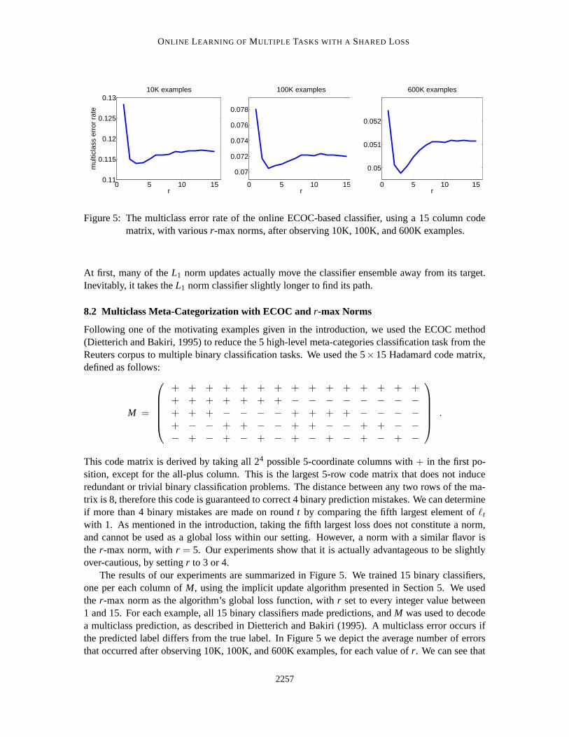
Figure 5: The multiclass error rate of the online ECOC-based classifier, using a 15 column codematrix, with various r-max norms, after observing 10K, 100K, and 600K examples.

At first, many of the L1 norm updates actually move the classifier ensemble away from its target.Inevitably, it takes the L1 norm classifier slightly longer to find its path.

8.2 Multiclass Meta-Categorization with ECOC and r-max Norms

Following one of the motivating examples given in the introduction, we used the ECOC method(Dietterich and Bakiri, 1995) to reduce the 5 high-level meta-categories classification task from theReuters corpus to multiple binary classification tasks. We used the 5× 15 Hadamard code matrix,defined as follows:

M =

+ + + + + + + + + + + + + + ++ + + + + + + − − − − − − − −+ + + − − − − + + + + − − − −+ − − + + − − + + − − + + − −− + − + − + − + − + − + − + −

.

This code matrix is derived by taking all 24 possible 5-coordinate columns with + in the first po-sition, except for the all-plus column. This is the largest 5-row code matrix that does not induceredundant or trivial binary classification problems. The distance between any two rows of the ma-trix is 8, therefore this code is guaranteed to correct 4 binary prediction mistakes. We can determineif more than 4 binary mistakes are made on round t by comparing the fifth largest element of `t

with 1. As mentioned in the introduction, taking the fifth largest loss does not constitute a norm,and cannot be used as a global loss within our setting. However, a norm with a similar flavor isthe r-max norm, with r = 5. Our experiments show that it is actually advantageous to be slightlyover-cautious, by setting r to 3 or 4.

The results of our experiments are summarized in Figure 5. We trained 15 binary classifiers,one per each column of M, using the implicit update algorithm presented in Section 5. We usedthe r-max norm as the algorithm’s global loss function, with r set to every integer value between1 and 15. For each example, all 15 binary classifiers made predictions, and M was used to decodea multiclass prediction, as described in Dietterich and Bakiri (1995). A multiclass error occurs ifthe predicted label differs from the true label. In Figure 5 we depict the average number of errorsthat occurred after observing 10K, 100K, and 600K examples, for each value of r. We can see that

2257


0 2 4 6 8x 10

5

0.4

0.5

0.6

0.7

0.8

online rounds

∞−

erro

r ra

te

∞−norm perceptron ∞−norm implicit

0 2 4 6 8x 10

5

0.005

0.01

0.015

0.02

0.025

online rounds

1−er

ror

rate

∞−norm perceptron ∞−norm implicit

Figure 6: The ∞-error (left) and 1-error (right) attained by the multitask Perceptron (dashed) andthe implicit update algorithm (solid) when using the L∞ norm as a global loss function.

using either the L1 norm (r = 15) or the L∞ norm (r = 1) is suboptimal, and the best performanceis consistently reached by setting r to be slightly smaller than half the code distance. Althoughthe theoretically motivated choice of r = 5 is not the best, it still yields better results than the twoextreme choices, r = 1 and r = 15.

When we replaced the Hadamard code matrix with the One-vs-Rest code matrix, defined by2I − 1 (where I is the 5× 5 identity matrix and 1 is the 5× 5 all-ones matrix) then the multiclasserror after observing 600K examples increases from 5% to around 8%. This justifies using theECOC method in the first place.

We conclude this experiment by noting that although setting r = 1 produces the largest numberof multiclass prediction mistakes, it still delivers the best performance if we evaluate the 15 classifierensemble using the ∞-error defined above.

8.3 The Implicit Update vs. the Multitask Perceptron

From a loss minimization standpoint, Theorem 9 proves that the implicit update, presented in Sec-tion 5, is at least as good as the multitask Perceptron variants, presented in Secs. 3 and 4. Thefollowing experiment demonstrates that the implicit update is also superior in practice.

We repeated the multitask multi-label experiment described in Section 8.1, using the multitaskPerceptron in place of the implicit update algorithm. The infinite horizon extension discussed inSection 4 does not have a significant effect on empirical performance, so we consider only the finitehorizon version of the multitask Perceptron, described in Section 3.

When the global loss function is defined using the L1 norm, both the implicit update and themultitask Perceptron update decouple to independent updates for each individual task. In this case,both algorithms are very similar, their empirical performance is almost identical, and the comparisonbetween them is not very interesting. Therefore, we focus on a global loss defined by the L∞ norm.

A comparison between the performance of the implicit update and the multitask Perceptronupdate, both using the L∞-norm loss, is given in Figure 6. The plot on the left-hand side of thefigure compares the two algorithms’ ∞-error-rate, and the plot on the right-hand side of the figure

2258


compares their 1-error-rate. The implicit algorithm holds a clear lead over the multitask Perceptronwith respect to both error measures, throughout the learning process. These results give empiricalvalidation to the formal comparison of the two algorithms.

9. Discussion

When faced with several online tasks in parallel, it is not always best to distribute the learning effortevenly. In many cases, it may be beneficial to allocate more effort to tasks when they are seen toplay “key” roles. In this paper, we presented an online algorithmic framework that does preciselythat. The priority given to each task is governed by its relative performance and by the choice of aglobal loss function.

We presented three families of algorithms, each of which includes an algorithm for every globalloss defined by an absolute norm. The first two families are illustrative and theoretically appeal-ing. The third family of algorithms uses the most sophisticated update of the three, and is the onerecommended for practical use. We demonstrated the superior performance of the third family ofalgorithms empirically.

We showed that, in the worst case, the finite horizon multitask Perceptron of Section 3 andthe implicit update algorithm of Section 5 both perform asymptotically as well as the best fixedhypothesis ensemble. In other words, these algorithms are no-regret algorithms with respect to anyglobal loss function defined by an absolute norm. The same cannot be said for the naive alternative,where we use multiple independent single-task learning algorithms to solve the multitask problem.We also demonstrated the benefit of the multitask approach over the naive alternative on two large-scale text categorization problems.

Throughout the paper, we assumed that the multiple online tasks are perfectly synchronized,and that a complete k-tuple of examples is observed on every round. This is indeed the case in eachof the concrete examples described in the introduction and empirically tested in our experiments.However, in other real-world situations, this may not be the case. Namely, there could occur situ-ations where not all of the tasks are active on every single round. In other words, there may be asubset of “dormant tasks” on each round. For example, say that we are operating an online store andthat we have multiple registered customers. Each product in our store is represented by a featurevector, and we train an individual binary classifier for each of our customers. When costumer jvisits a product-page on our website, the respective classifier is used to predict whether that cus-tomer intends to purchase the product or not. The prediction is then used to decide whether or notto lure the customer away from that page. This setting induces a natural online multitask learningproblem. Moreover, only a fraction of the customers is online at any given moment. We considerthe tasks of those customers that are not online to be dormant or inactive tasks. At a first glance,the inactive tasks setting may seem to be more complicated than the fully synchronized setting dis-cussed throughout the paper. However, our algorithms and analysis accommodate this extensionquite naturally. We simply need to define `t, j = 0 for every inactive task and apply the multitaskupdate verbatim. Due to the conservativeness assumption, the hypotheses of the inactive tasks willbe left intact. Additionally, note that all of the norms discussed in this paper have the property that‖v‖ = ‖v′‖, where v′ is the vector obtained by removing all of the zero entries from v. Therefore,we can imagine that the length of the vector `t changes from round to round, and that the update oneach round is applied as if the tasks that are sleeping on that round never existed in the first place.We would also like to note that, although our presentation focuses on multiple binary classifica-

2259


tion tasks, our algorithms and techniques can be adapted to other online learning problems as well.Specifically, a multitask implicit update can be derived for regression and uniclass problems usingideas from Crammer et al. (2006).

The next-step would be to extend our framework from absolute norms to general norms. Forexample, the family of Mahalanobis norms, defined by ‖z‖2 = z>Pz (where P is a positive definitematrix) includes norms that are not absolute but which could have interesting applications in oursetting. More generally, there exist meaningful global loss functions which are not norms at all.

Another interesting research direction would be to return to the roots of statistical multitasklearning, and to try to model generative similarities between the multiple tasks within the onlineframework. In our work, we completely disregarded any relatedness between the multiple tasks, andonly considered the shared consequences of errors. In the game-theoretic spirit of online learning,modeling these similarities would have to be done without making statistical assumptions on thedata source.

Appendix A. The K-Method of Norm Interpolation

In this section, we briefly survey Peetre’s K-method of norm interpolation. This method takes apair of norms and smoothly interpolates between them, producing a new family of norms whichcan be used in our setting. An example of such an interpolation is the family of r-max norms,previously mentioned in this paper. The main practical purpose of this section is to prove that thedual of the r-max norm takes the form given in Equation (3). We do not present the K-method inall its generality, but rather focus only on topics which are relevant to the online multitask learningsetting. The interested reader is referred to Bennett and Sharpley (1998) for a more detailed accountof interpolation theory.

We begin by presenting Peetre’s K-functional and J-functional, and proving that they inducedual norms. Let ‖ ·‖p1 : R

k → R+ and ‖ ·‖p2 : Rk → R+ be two p-norms, and let ‖ ·‖q1 and ‖ ·‖q2 be

their respective duals. The K-functional with respect to p1 and p2, and with respect to the constantα > 0, is defined as

‖v‖K(p1,p2,α) = minw+z=v

(

‖w‖p1 +α‖z‖p2

)

.

The J-functional with respect to q1, q2, and with respect to the constant β > 0, is defined as

‖u‖J(q1,q2,β) = max{

‖u‖q1 , β‖u‖q2

}

.

The J-functional is obviously a norm: positivity and linearity follow immediately from the fact that‖ · ‖q1 and ‖ · ‖q2 posses these properties. The triangle inequality follows from

‖v+u‖J(q1,q2,β) = max{

‖v+u‖q1 , β‖v+u‖q2

}

≤ max{

‖v‖q1 +‖u‖q1 , β‖v‖q2 +β‖u‖q2

}

≤ max{

‖v‖q1 , β‖v‖q2

}

+ max{

‖u‖q1 , β‖u‖q2

}

= ‖v‖J(q1,q2,β) + ‖u‖J(q1,q2,β) .

Since the J-functional is defined with respect to two absolute norms, it too is an absolute norm.Instead of explicitly proving that ‖ · ‖K(p1,p2,α) is also a norm, we prove that it is the dual of

‖ ·‖J(q1,q2,β) when α = 1/β. Since the dual of an absolute norm is itself an absolute norm, and since

2260


the dual of the dual norm is the original norm (Horn and Johnson, 1985), our proof implies that‖ · ‖K(p1,p2,α) is indeed a norm, that it is absolute, and that its dual is ‖ · ‖J(q1,q2,1/α).

Theorem 10 Using the notation defined above,

‖ · ‖∗J(q1,q2,β) ≡ ‖ ·‖K(p1,p2,1/β) .

Proof We abbreviate ‖v‖J = ‖v‖J(q1,q2,β) and ‖v‖K = ‖v‖K(p1,p2,1/β) throughout the proof. First,we show that ‖v‖∗J ≤ ‖v‖K for all v ∈ R

k. Let v,w and z be vectors in Rk such that v = w+z. Then

for any u ∈ Rk, we can use Holder’s inequality to obtain

u ·v = u ·w + u · z≤ ‖u‖q1‖w‖p1 + ‖u‖q2‖z‖p2 .

By definition, it holds that

‖u‖q1 ≤ ‖u‖J and ‖u‖q2 ≤1β‖u‖J ,

and so

u ·v ≤(

‖w‖p1 +1β‖z‖p2

)

‖u‖J .

Since the only restriction on u,v,w and z is that v = w+ z, we can fix v, choose u to be the vectorwhich maximizes the left-hand side above subject to ‖u‖J ≤ 1, and choose w and z which minimizethe right-hand side above subject to v = w+ z. This results in

maxu∈Rk:‖u‖J≤1

u ·v ≤ minw+z=v

(

‖w‖p1 +1β‖z‖p2

)

.

The left-hand side above is the formal definition of ‖v‖∗J , the right-hand side is the definition of‖v‖K , and we have proven that ‖v‖∗J ≤ ‖v‖K .

To prove the opposite direction, fix v and let u be the vector with ‖u‖J ≤ 1 which maximizesu ·v. We now consider two cases. If ‖u‖q1 ≥ β‖u‖q2 then

‖v‖∗J = maxu:‖u‖q1≤1

u ·v .

Using the duality of ‖ · ‖q1 and ‖ · ‖p1 , the right hand-side above equals ‖v‖p1 . Since we can choosew = v and z = 0, it certainly holds that

‖v‖p1 ≥ minw+z=v

(

‖w‖p1 +1β‖z‖p2

)

= ‖v‖K .

On the other hand, if ‖u‖q1 ≤ β‖u‖q2 then

‖v‖∗J =1β

maxu:‖u‖p2≤1

u ·v .

2261


Using the duality of ‖·‖q2 and ‖·‖p2 , the right hand-side above equals 1β‖v‖p2 . Since we can choose

w = 0 and z = v, it holds that

1β‖v‖p2 ≥ min

w+z=v

(

‖w‖p2 +1β‖z‖p2

)

= ‖v‖K .

Overall, we have shown that ‖v‖∗J ≥ ‖v‖K .

The r-max norm discussed in the paper is an instance of the K-functional, and can be defined as

‖v‖r-max = ‖v‖K(1,∞,r) .

To see why this is true, let φ be the absolute value of the r’th absolutely largest coordinate in v. Nowdefine for each 1 ≤ j ≤ k

w j = sign(v j)max{0, |v j|−φ} and z j = sign(v j)min{|v j|,φ} .

Note that w+ z = v, and that‖v‖r-max = ‖w‖1 + r‖z‖∞ .

This proves that ‖v‖r-max ≥ ‖v‖K(1,∞,r).Turning to the opposite inequality, let π(1), . . . ,π(r) be the indices of the r absolutely largest

elements of v, and let w and z be vectors such that w+ z = v. We now have that

‖v‖r-max =r

∑j=1

|vπ( j)|

=r

∑j=1

|wπ( j) + zπ( j)|

≤r

∑j=1

|wπ( j)| +r

∑j=1

|zπ( j)|

≤r

∑j=1

|wπ( j)| + r maxj=1,...,r

|zπ( j)|

≤k

∑j=1

|w j| + r maxj=1,...,k

|z j| = ‖w‖1 + r‖z‖∞ .

The above holds for any w and z which sum to v, and specifically to those which minimize ‖w‖1 +r‖z‖∞. We conclude that ‖v‖r-max ≤ ‖v‖K(1,∞,r), and therefore ‖v‖r-max = ‖v‖K(1,∞,r).

Finally, we calculate an upper bound on the remoteness of ‖·‖J(q1,q2,β). This enables us to obtainconcrete loss bounds for interpolation norms from the theorems proven in this paper. Recall that

ρ(‖ · ‖J(q1,q2,β),k) = maxu∈Rk

‖u‖2

‖u‖J(q1,q2,β).

Using the definition of the J-functional, the above becomes

maxu∈Rk

min

{ ‖u‖2

‖u‖q1

,‖u‖2

β‖u‖q2

}

.

2262


Using the weak minimax theorem, we can upper-bound the above by

min

{

maxu∈Rk

‖u‖2

‖u‖q1

,maxu∈Rk

‖u‖2

β‖u‖q2

}

.

Once again using the definition of remoteness, the above can be rewritten as

min

{

ρ(‖ · ‖q1 ,k),ρ(‖ · ‖q2 ,k)

β

}

.

Using Lemma 2, we can obtain an explicit upper bound on the remoteness of any interpolation ofp-norms.

References

J. Baxter. A model of inductive bias learning. Journal of Artificial Intelligence Research, 12:149–198, 2000.

S. Ben-David and R. Schuller. Exploiting task relatedness for multiple task learning. In Proceedingsof the Sixteenth Annual Conference on Computational Learning Theory, 2003.

C. Bennett and R. Sharpley. Interpolation of Operators. Academic Press, 1998.

S. Boyd and L. Vandenberghe. Convex Optimization. Cambridge University Press, 2004.

R. Caruana. Multitask learning. Machine Learning, 28(1):41–75, 1997.

O. Chapelle and Z. Harchaoui. A machine learning approach to conjoint analysis. In Advances inNeural Information Processing Systems, volume 17, 2005.

K. Crammer and Y. Singer. On the algorithmic implementation of multiclass kernel-based vectormachines. Journal of Machine Learning Research, 2:265–292, 2001.

K. Crammer and Y. Singer. Ultraconservative online algorithms for multiclass problems. Journalof Machine Learning Research, 3:951–991, 2003.

K. Crammer, O. Dekel, J. Keshet, S. Shalev-Shwartz, and Y. Singer. Online passive aggressivealgorithms. Journal of Machine Learning Research, 7:551–585, Mar 2006.

T. G. Dietterich and G. Bakiri. Solving multiclass learning problems via error-correcting outputcodes. Journal of Artificial Intelligence Research, 2:263–286, January 1995.

T. Evgeniou, C.Micchelli, and M. Pontil. Learning multiple tasks with kernel methods. Journal ofMachine Learning Research, 6:615–637, 2005.

D. P. Helmbold, J. Kivinen, and M. Warmuth. Relative loss bounds for single neurons. IEEETransactions on Neural Networks, 10(6):1291–1304, 1999.

R. Herbrich, T. Graepel, and K. Obermayer. Large marging rank boundaries for ordinal regression.In A. Smola, B. Scholkopf, and D. Schuurmans, editors, Advances in Large Margin Classifiers.MIT Press, 2000.

2263


T. Heskes. Solving a huge number of silmilar tasks: A combination of multitask learning anda hierarchical bayesian approach. In Proceedings of the Fifteenth International Conference onMachine Learning, pages 233–241, 1998.

R. A. Horn and C. R. Johnson. Matrix Analysis. Cambridge University Press, 1985.

J. Kivinen and M. Warmuth. Relative loss bounds for multidimensional regression problems. Jour-nal of Machine Learning, 45(3):301–329, July 2001.

A. B. J. Novikoff. On convergence proofs on perceptrons. In Proceedings of the Symposium on theMathematical Theory of Automata, volume XII, pages 615–622, 1962.

F. Rosenblatt. The perceptron: A probabilistic model for information storage and organization inthe brain. Psychological Review, 65:386–407, 1958. (Reprinted in Neurocomputing (MIT Press,1988).).

I. Tsochantaridis, T. Hofmann, T. Joachims, and Y. Altun. Support vector machine learning forinterdependent and structured output spaces. In Proceedings of the Twenty-First InternationalConference on Machine Learning, 2004.

2264

Documents

Online Learning of Multiple Tasks with a Shared Loss