Online Filtering, Smoothing and Probabilistic Modeling ofStreaming data

Bhargav Kanagal Amol Deshpandebhargav@cs.umd.edu amol@cs.umd.edu

University of Maryland University of Maryland

Abstract

In this paper, we address the problem of extending a relational database system to facilitate efficientreal-time application of dynamic probabilistic models to streaming data. We use the recently proposedabstraction of model-based views for this purpose, by allowing users to declaratively specify the modelto be applied, and by presenting the output of the models to the user as a probabilistic database view. Wesupport declarative querying over such views using an extended version of SQL that allows for queryingprobabilistic data. Underneath we use particle filters, a class of sequential Monte Carlo algorithmscommonly used to implement dynamic probabilistic models, to represent the present and historical statesof the model as sets of weighted samples (particles) that are kept up-to-date as new readings arrive.We develop novel techniques to convert the queries on the model-based view directly into queries overparticle tables, enabling highly efficient query processing. Finally, we present experimental evaluation ofour prototype implementation over sensor data from the Intel Lab dataset that demonstrates the feasibilityof online modeling of streaming data using our system and establishes the advantages of such tightintegration between dynamic probabilistic models and database systems.

1 Introduction

Enormous amounts of streaming data are being generated everyday by measurement infrastructures thatcontinuously monitor a variety of things from environmental properties using sensor networks [29] to be-havior of large computational clusters [19]. To fully harvest the benefits of this extensive monitoring, wemust be able to process and analyze such data streams in real-time. In recent years, there has been muchwork on data stream management systems [6, 7, 5, 31] that can process high-rate data streams in real-timeand continuously evaluate SQL queries over them. A large class of commonly used stream processing tasks,however, cannot be expressed as SQL queries and thus cannot benefit from these advances in stream dataprocessing. Examples of such tasks include:

• Inferring hidden variables: In several real-world data streams, the attributes of interest may not bedirectly observable (e.g. working status of a remotely located wireless sensor), or it may be very expensiveto measure them (light on a Berkeley Mote [12]). A common processing task over such data streams is tocontinuously infer the value of the hidden variables using the observed data. Hidden Markov models [36],or variations thereof, are often used for this purpose. These types of models allow us to combine priordomain knowledge about the system behavior with the actual observations to compute the most likelyvalues of the hidden variables (Section 2.1).

1

• Eliminating measurement noise: Data Streams generated by distributed measurement infrastructureslike sensor networks or GPS devices, are invariably noisy; this could be because of calibration effects(e.g., temperature sensors typically report voltages that are then converted into Celsius), errors due topoor coupling or analog-to-digital conversion, inaccuracies due to non-robust measurement techniquesthat fail in harsh environments (e.g., multi-path propagation errors that occur in GPS in urban settings),or inherent flaws with mass-produced sensing devices. Removing measurement noise is perhaps the mostimportant first step when analyzing such data streams or processing user queries over them. Analyticalfiltering techniques such as Kalman filters [43] (Section 2.2), and its extensions like extended Kalmanfilters and unscented Kalman filters, are commonly used for this purpose in a wide variety of domains.

• Probabilistically modeling high-level events from low-level sensor readings: Automatically recogniz-ing higher level events such as user activities through use of unobtrusive sensing technologies is consid-ered a key in the field of Ubiquitous computing [9, 34, 26]. For instance, Patterson et al. [34] demonstratehow the transportation mode of a user can be learned using GPS readings, which they then use to designa guiding device for cognitively impaired people. Increasing deployments of large-scale sensing infras-tructures will enable many such applications in the near future. Ideally, we would like to perform thistype of modeling in real-time as the data is being generated and streamed into the system; the applicationdevelopers can then be provided access to these inferred events (subject to privacy policies) directly in astreaming fashion, so they can provide user services.

There are several other common stream processing tasks such as predictive modeling and extrapolation tofill up missing values, identifying temporal or spatial trends and patterns in the data, novelty and anomalydetection and so on, that cannot be expressed as SQL queries. In most such applications, the majorityof the analysis and querying is typically done outside the database system, leading to much repetition offunctionality and highly inefficient execution. We start by presenting a motivating application in detail inthe following subsection.

1.1 Motivating Application

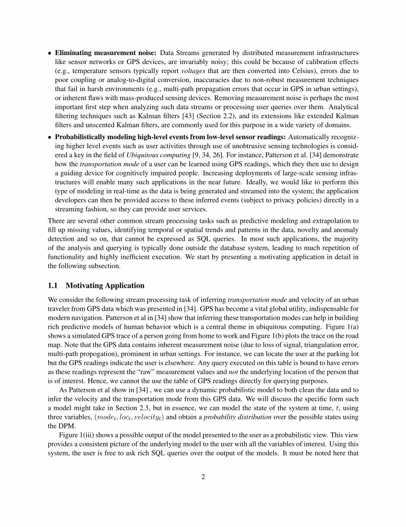
We consider the following stream processing task of inferring transportation mode and velocity of an urbantraveler from GPS data which was presented in [34]. GPS has become a vital global utility, indispensable formodern navigation. Patterson et al in [34] show that inferring these transportation modes can help in buildingrich predictive models of human behavior which is a central theme in ubiquitous computing. Figure 1(a)shows a simulated GPS trace of a person going from home to work and Figure 1(b) plots the trace on the roadmap. Note that the GPS data contains inherent measurement noise (due to loss of signal, triangulation error,multi-path propogation), prominent in urban settings. For instance, we can locate the user at the parking lotbut the GPS readings indicate the user is elsewhere. Any query executed on this table is bound to have errorsas these readings represent the “raw” measurement values and not the underlying location of the person thatis of interest. Hence, we cannot the use the table of GPS readings directly for querying purposes.

As Patterson et al show in [34] , we can use a dynamic probabilistic model to both clean the data and toinfer the velocity and the transportation mode from this GPS data. We will discuss the specific form sucha model might take in Section 2.3, but in essence, we can model the state of the system at time, t, usingthree variables, (modet, loct, velocityt) and obtain a probability distribution over the possible states usingthe DPM.

Figure 1(iii) shows a possible output of the model presented to the user as a probabilistic view. This viewprovides a consistent picture of the underlying model to the user with all the variables of interest. Using thissystem, the user is free to ask rich SQL queries over the output of the models. It must be noted here that

2

Time Positionx y

. . . . . . . . .22 32.89 34.4023 32.93 32.2324 - -25 57.07 48.0126 65.49 53.8627 - -28 - -29 106.4 80.030 107.12 80.5131 107.12 80.51. . . . . . . . .(a) Input GPS Data (b) Plot of GPS trace

Time Position Velocity Modex y vx vy

. . . . . . . . . . . . . . . . . .22 32.50 35.45 0.15 2.50 Walking23 32.50 32.20 0.08 2.45 Walking24 44.50 40.5 12.5 8.3 Driving25 56.56 48.25 11.0 8.2 Driving26 68.54 56.5 12.3 8.1 Driving27 80.32 64.5 12.5 7.9 Driving28 92.44 72.5 12.1 8.5 Driving29 104.4 80.5 12.5 8.1 Driving30 106.50 80.5 2.1 0.22 Walking31 108.8 80.8 2.1 0.3 Walking. . . . . . . . . . . . . . . . . .

(c) Output Probabilistic View (Our System)

Figure 1: (a,b) GPS trace of the urban traveler traveling from home to work. (c) The output of a dynamicprobabilistic model (used to both clean the GPS data and to infer the velocity and transportation mode) canbe presented as a user-queriable deterministic database table.

queries can also be posed on velocity and the mode, which were the hidden attributes inferred using theDBN.

In this paper, we present an extensible system that exploits the commonalities between many of thesetasks to natively support them inside a relational database system. Most of the aforementioned tasks canbe seen as applications of specific instances of dynamic probabilistic models (DPMs) to streaming data [33,

3

30]1. We use the recently proposed abstraction of model-based views [13] to push the application of a widerange of DPMs to streaming data inside a relational DBMS, thus enabling easy application of these tasks.

1.2 Contributions

The salient contributions of our work are as follows:• We extend the abstraction of model-based views [13] to present the output of a DPM to the users as

probabilistic tables, leading to intuitive user interaction with the system.

• We exploit the structure of particle filters (a widely-applicable sequential Monte Carlo inference tech-nique) to efficiently store the probabilistic output of a DPM as a set of weighted samples (called parti-cles). Our internal representation also naturally captures many of the attributes correlations present in thedata.

• We design novel techniques to convert queries posed over a single DPM-based view (including aggregatequeries) into queries over our internal particle-based representation, allowing us to exploit the existingquery processing machinery.

• Our experimental results show that we can achieve sufficient accuracy with a few particles (about 100)and that the time taken to process large number of particles (about 1000) is quite reasonable. This makesour system feasible for online modeling of streaming data.

The rest of the paper is organized as follows. We begin with an overview of dynamic probabilistic models inSection 2. We describe the abstraction of DPM-based views in Section 3 and present a detailed descriptionof our system and the algorithms used in Sections 4-8. We conclude with an experimental evaluation of ourprototype implementation in Section 9.

2 Dynamic Probabilistic Models

Dynamic probabilistic models are widely used in practice to model complex real-world stochastic pro-cesses and to reason about them. They form an active area of research in the machine learning commu-nity [22, 16, 33, 18, 30] and are playing an increasingly important role in the design of machine learning al-gorithms. The simplest and most widely used examples of dynamic probabilistic models are hidden Markovmodels (HMMs) and linear dynamical systems (better known as Kalman filter models (KFMs)). We illus-trate dynamic probabilistic models by describing some of the simple applications of HMMs and KFMs andthen describe a generalized graphical representation for DPMs.

2.1 Hidden Markov Models

Hidden Markov models (HMMs) are used in a variety of applications like speech recognition [36], bioin-formatics [15] and fault detection [23, 46]. In short, HMMs are used to infer the values of unobservable(hidden) state variables from the imprecise observations that are made about related variables.

We will illustrate HMMs using a simple fault detection application. Fault detection in mass produced,low cost sensor nodes is an important research problem and is widely studied in literature [23, 38, 46]. Letus consider an example of a single sensor, possibly faulty, that is measuring temperatures in a room andtransmitting them to a central database server. We want to know whether the sensor is working correctly

1 In this paper, we assume that DPMs are equivalent to the class of dynamic Bayesian networks. In some literature, DPMs areconsidered to be a more general class of models than the ones we consider here.

4

p(Tt|Tt−1, St) ={N(Tt−1, σ) St = WoU(min,max) St = Fa

p(St+1|St) =Wo Fa

Wo 0.99 0.01Fa 0.01 0.99

p(Vt+1|Vt) = N(Vt, σV )p(Xt+1|Xt, Vt+1) =

N(Xt + Vt+1, σX)p(Zt+1|Xt+1) = N(Xt+1, σY )Priors : p(V0) and p(X0)

(i) AR-HMM 2 (ii) KFM

Figure 2: Graphical representations of DPMs. (i) Using an HMM for fault detection; (ii) Using a KFM forvelocity and location estimation.

(so that we could ignore the erroneous readings produced by faulty sensors). The only information we haveabout the sensor are the temperature readings it transmits. We can use an HMM to infer the sensor’s statusfrom these readings alone. In this example, the hidden variable (that we cannot measure) is the status ofthe sensor, which can be in two states, Working (Wo) or Failed (Fa). The observed readings are thetemperatures measured by the device.

Figure 2(i) shows the graphical representation of the HMM we can use to model the state of such asystem. The shaded node denotes the observed temperature at time t (denoted by Tt), whereas the unshadednode denotes the hidden status variable that captures whether the sensor is working or not (denoted by St).The prior knowledge about the behavior of the system (that is used to determine whether the sensor hasfailed) can be captured by three conditional probability distributions:• P (Tt+1|Tt, St+1 = Working): This distribution captures the expected behavior of the sensor when the

sensor is functioning correctly. For instance, from prior knowledge about the process, we expect that attime t + 1, the sensor should return values around Tt plus a small (Gaussian) noise. This distributioncan also be learned from historical data.

• P (Tt+1|Tt, St+1 = Faulty): This distribution captures the expected behavior when the sensor is faulty.One simple way to model something like this would be to assume that the sensor might return any valuefrom 0 to 100 uniformly independently of the actual temperature. Clearly the faulty behavior dependson the nature of the sensor.

• P (St+1|St): Figure 2(i) shows a possible table for this that captures the prior knowledge that the sensorhas a small probability of failing. The table indicates that if the sensor was working at time t, then theprobability that it will fail in the next time instant is 0.01 and if the sensor has failed now, the probabilitythat it will work the next time instant is 0.01. Once again, the actual probabilities depend on the nature of

2AR-HMMs (Auto-Regressive HMMs) are a specific class of HMMs.

5

the sensor and possibly the manufacturing process; for most devices, this type of information is typicallyavailable.

These conditional distributions form the parameters of the HMM. By combining them with the observedtemperatures from the data stream, HMMs provide mechanisms to infer the best possible estimate of thehidden variables (in our case, the status of the sensor at various times) using the observed measurements.Some of the common analytical algorithms used for this purpose are forward-backward and Vitterbi algo-rithms [36]. These algorithms can be seen as special cases of general inference algorithms designed fordynamic probabilistic models [40]; we describe one such inference technique in Section 6.1.

We would like to note that this model is not appropriate for predicting future temperature values fromcurrent temperature and is appropriate only for fault detection. A model that can be used to predict futuretemperatures is shown in Figure 3(i).

2.2 Linear Dynamical Systems

A linear dynamical system, more commonly known as the Kalman filter model (KFM), is another widelyused dynamic probabilistic model. We illustrate KFMs using the following application. We are interestedin computing the position and velocity of a car based on continuous observations of the position of the carmade by an inaccurate GPS device.

Here, velocity is a hidden variable that is not being measured directly. Furthermore, the actual positionis also not known because of the inherent measurement noise in GPS data. In this case the state of the carat time t is denoted by [xt, vt], where xt denotes the true location of the car (assuming one-dimensionalmotion) and vt denotes the velocity. Let zt denote the observed location of the car.

Figure 2(ii) shows a pictorial representation of the KFM that can be used in this application. (Thismodel was described by Murphy [33]). Similar to the earlier example, we can summarize our prior knowl-edge about the process using the following equations; these equations can be easily recast as conditionalprobability distributions (shown in Figure 2(ii)).

zt = xt +N (0,W1)xt+1 = xt + vt+1 +N (0,W2)vt+1 = vt +N (0,W3)

The first equation specifies how the measurement noise (which is assumed to be a zero-mean Gaussian withcovariance W1) affects the observed locations, whereas the latter two equations encode the movement of theobject and the random perturbations that the location and velocity might be subject to.

Kalman filter actually refers to a specific analytical inference algorithm for the LDS model [43]. Giventhe observed variables and the conditional distributions, this algorithm can be used to obtain a distributionover the hidden variables (velocity and true location in our case) and once again, it can be seen as a specialcase of general inference algorithms for DPMs [25]. We will continue to call this model the Kalman filtermodel (KFM).

2.3 DPMs & Graphical representation

Generally speaking, a dynamic probabilistic model (DPM) is used to compactly represent the stochastic evo-lution of a set of random variables over time [16]. DPMs are typically represented using a directed graphicalstructure as shown in Figure 3(i), where the graph structure captures the complex interdependencies betweenthe variables of the process. We will illustrate the graphical representation using the model shown in Figure

6

Figure 3: (i) Graphical representation of the BBQ DPM used for modeling Intel Lab data (Section 9); (ii) Ageneric DPM used for Transporation Mode Estimation application discussed in Section 1.

3(i), which we call “BBQ DPM” [12]. This model is used to infer hidden temperature values using observedhumidity values in a sensor network and also remove noise from the observed humidity values (Section9). Figure 3(ii) is another generic DPM that can be used for the transportation mode estimation examplediscussed in Section 1. The details of the graphical representation are illustrated below.

Nodes: The nodes of the graph represent the attributes of the system being modeled (that are modeled asrandom variables). In Figure 3(i), the attributes of the system being modeled are temperature Tt and humid-ity Ht. The measured humidity Mt and hour of the day hourt are observed quantities. By convention, theobserved nodes are shaded while the hidden nodes are clear.

Edges: The directed edges represent “causality”. In Figure 3(i), the temperature at time t influences thetemperature at time t+ 1. Similarly the temperature at time t influences the humidity at time t. The degreeof causality is indicated by the conditional probability distribution function (CPD). The CPD of node X isindicated by P (X|Pa(X)) where Pa(X) denotes the parents of node X .

Time: Time is represented in a DPM through use of vertical slices. Each vertical slice of the graphicalmodel corresponds to the state of the system at a given time instant. As time advances, we can unroll themodel by repeating the structure and parameters of the model as shown in Figures 3 (i),(ii).

CPD: The key parameters of a DPM are the conditional probability distributions that encode our knowledgeabout the system being monitored, and its evolution over time. We need three sets of probability distributionsto fully specify a DPM:• The prior (unconditional) probability distributions over the variables in the first slice (that may not have

any parents).

• The conditional probability distributions that encode the knowledge about how the state at time t + 1depends on the state at time t.

• The conditional probability distributions that encode the knowledge about the how the observation attime t depends on the state at time t.

7

Figure 4: Abstraction of model-based views

Typically it is assumed that the variables at time t depend directly only on the variables at time t andt− 1 (Markov assumption), and hence a 2-slice representation (as shown in Figures 2(i) and (ii)) is usuallysufficient. In Figure 3(i), the CPD of node Tt+1 depends on Tt and the hour of the day ht+1. This isbecause hourly change in temperature depends on the hour of the day. Temperature increases during theday, decreases at night by a magnitude that also depends on the hour. The CPD of the humidity node Ht issimilar.

2.3.1 Inference

The ultimate goal of modeling a stochastic process using a DPM is to obtain a posterior distribution overthe hidden variables of the graphical model, given the observed measurements. This task is called inference.Several inference algorithms have been developed for efficient inference in special cases (e.g. KalmanFilters), and many general purpose inference techniques (e.g. junction tree algorithm) are also known. Wepresent one such general purpose algorithm, based on Monte Carlo techniques, in Section 6.1. The outputof the inference algorithm is typically a probability distribution over the hidden variables (although someinference algorithms may only provide expected or most likely values of the hidden variables).

2.3.2 Learning

The CPD parameters of the DPM are typically not known to the user and hence need to be learned fromtraining data. Maximum Likelihood Estimation (MLE) is one of the popular statistical methods used forlearning parameters of the CPDs. Given learning data, MLE estimates the values of the parameter values, θthat maximizes the likelihood of observing the learning data. In other words, we determine the parameter θthat makes the learning data “most likely”. Details of MLE are described in Section 7.

In the next section, we present our proposal for presenting the output of a DPM to the users.

3 DPMs as Database Views

We use the abstraction of model-based views, proposed in our prior work [13], to present the output of aDPM to the users. This abstraction is analogous to the well-known abstraction of database views whichallows creating virtual tables using an SQL query over one or more database tables. Model-based views

8

time (t) temp Tt humidity Ht...

......

3

4

5...

......

SID time temp humidity weight...

......

......

1 4 21.43 40.60 0.402 4 21.48 40.50 0.203 4 21.49 40.51 0.054 4 20.21 41.51 0.155 4 21.62 40.29 0.20...

......

......

(a) DPM based view (b) Associated Particle Table

Figure 5: (a) DPM-based views contain probabilistic attributes; (b) Particle-based representation of the view(only particles corresponding to the second tuple, time = 4, are shown for clarity)

further this abstraction and allow creating such virtual tables using a statistical model instead (Figure 4).Several examples of model-based views based on non-parametric statistical models like linear regressionand interpolation are described in [13].

We extend this abstraction by allowing views to be defined using DPMs instead. Figure 5(a) shows theschema of the view that would be presented to the user with the BBQ DPM model (Section 2.3) that inferstemperature from observed humidity values. As we can see, the schema contains all the state variables inthe DPM as attributes along with a time attribute. As with traditional database views, this is a virtual tableand it may or may not be materialized.

Note that the nature of DPMs forces these to be probabilistic views in that the attributes of this virtualtable may be probabilistic. For instance, in Figure 5(a), the temperature attribute is not known with certaintysince the DPM only provides a probability distribution over it. Although the above DPM based view showsonly continuous variables, DPM views can also have discrete variables. (e.g. status attribute in HMM basedview presented to the user in the Fault detection example (Section 2.1)).

The issue of querying and representing such probabilistic data has received much attention in recentyears [4, 24, 8, 44, 11, 2, 39], and some of the challenges we face form active research focuses in that area.We plan to utilize the techniques developed in that work to a large extent in building our system, especiallylanguage extensions for querying such tables. We currently allow querying single table DPM-based viewsusing an extended version of SQL with the following features:

• µ(X): We allow the users to specify operations on the expected values of probabilistic attributes usingthis extensions. Thus, a predicate such as µ(temp) > 30 indicates that the condition is on the meanvalue of the temperature attribute.• with confidence c: This construct allows the users to specify a minimum confidence in the result

tuples returned to the users.• We allow queries with aggregates such as AVG, MIN, MAX and NN (Nearest Neighbor).• Although the query processing itself is cognizant of the probability distributions and the correlations,

if the attributes of the final result are probabilistic, the user is presented with either the expected values(µ) or the most likely values (in case of discrete attributes) instead.

One significant way DPM-based views differ from prior work in this area is that DPM-based views exhibitcomplex and strong attribute correlations that can not be ignored during query processing. Most of the prob-abilistic databases either assumes independence or severely restrict the correlations that can be represented.

9

We differentiate between two types of correlations:

• intra-tuple correlations: that exist between attributes of a single tuple. For example, in Figure 5(a),humidity and the temperature attributes are correlated.• inter-tuple correlations: that exist between attributes of different tuples. For example, temperatures

at times t and t+ 1 are likely to be highly correlated with each other.

Our internal representation (that we discuss next) currently captures the intra-tuple correlations, and thequery results are also affected by it. Inter-tuple correlations, on the other hand, are harder to capture and wecurrently ignore those during query processing; in future, we plan to develop intuitive ways of representingand querying such correlations.

3.1 Particle-based representation

We use a representation based on weighted samples (called particles) to store the DPM-based views inter-nally. This not only allows us to handle the complex, continuous, and correlated probability distributionsthat may be generated during probabilistic modeling, but also forms the basis for our inference technique.

Definition: A particle is a weighted sample drawn from a probability distribution. The weight associatedwith the sample represents its likelihood of occurence in the distribution.

To represent a DPM-based view as a relational table with deterministic attributes, we essentially maintain aset of particles for each tuple in the view. These particles are drawn from the joint distribution over all theattributes in the view. Figure 5(b) shows an example set of particles corresponding to one of the tuples in theview. Clearly the accuracy of such a representation depends on the number of particles used (N , a systemparameter). It can be shown theoretically that the accuracy of the representation is proportional to 1/N [14].The schema of this table, called particle table, consists of the attributes of the view along with a SampleIDattribute (SID), and a weight attribute.

Given such a particle table, the expected (or most likely) values of the attributes are computed by takingweighted averages over the particles. For example, the expected value of the temperature attribute at time4 is given by (Figure 5(b)):

T4 =N∑

i=1

(T i4 ∗ wi

4) = 21.43 ∗ 0.4 + · · ·+ 21.62 ∗ 0.2 = 21.28

Similarly, we can compute expected value of humidity attribute. Since the particles are drawn from the jointdistribution, the intra-tuple correlations are naturally captured in this representation.Populating the Particle TablesAt the start of the process (at time = 0), the particle table is initially populated by sampling over the priordistributions of the attributes. After that, the particles are directly generated, and in some cases updated, bythe inference algorithm that we use (Section 6).

4 System Design

The schematic diagram depicting the architecture of our system is shown in Figure 6. Suppose that the useris interested in modeling a data stream based on a suitable probabilistic model. The following sequence ofsteps occur, we will look at each of the operations in detail.

10

Figure 6: Architecture of our system

1. The user issues a request to the View Manager to create the DPM based view by providing a createview definition statement (Section 4.1). This specifies the DPM to be used, data stream to be modeled,training data to learn the DPM.

2. If the parameters are to be learned using training data, the learning module is invoked over the trainingdata (Section 7).

3. A particle table is created and populated using the prior distributions specified along with the viewdefinition (Section 3.1).

4. The user interacts with the DPM based view by issuing SQL-style queries (extended to deal withprobabilistic data). A query transformer intercepts these queries and converts them into SQL queriesover the particle table that are then executed using the traditional query processor (Section 5).

5. The particle table is continuously updated by the Update Manager in order to keep it consistent withthe incoming data stream (Section 6.1)

4.1 Specifying DPM-based Views

To create a DPM-based view over a stream, the user is required to specify the following details:– The schema of the view.– The data stream to be modeled.– The dynamic probabilistic model (DPM) to be used to model the data.The generic view definition statement to create a DPM-based view is as follows.

CREATE VIEW <name of view> <Schema> AS

DPM <DPM config in file>

<TRAINING DATA <SQL query for training data>>

STREAMING DATA <SQL query for streaming data>

11

# Node PropertiesnumNodes: 4hidden: {1,3}discrete: {1,3}node(1): [’Wo’ ’Fa’]node(3): [’Wo’ ’Fa’]

# Graph adjacency matrixgraph: [0 1 1 0;

0 0 0 1;0 0 0 1;0 0 0 0]

# CPDs of Nodescpd(1):[1;0];cpd(2):(val(1),[N(50,0.05);

U(-100,+100)]);cpd(3):(val(1),[[0.99;0.01];

[0.01;0.99]]);cpd(4):(val(3),[N(val(2),0.05);

U(-100,+100)]);

# Node PropertiesnumNodes: 6hidden: {1,2,4,5}discrete: {}

# Graph adjacency matrixgraph: [0 1 0 1 0 0;

0 0 1 0 0 0;0 0 0 0 0 0;0 0 0 0 1 0;0 0 0 0 0 1;0 0 0 0 0 0]

# CPDs of nodescpd(1): N(0,0.05);cpd(2): N(0,0.05);cpd(3): N(val(2),0.05);cpd(4): N(val(1),0.05);cpd(5): N(val(4)+val(2),0.05);cpd(6): N(val(5),0.05);

(i) Configuration file for the HMM model (ii) Configuation file for the KFM model

Figure 7: (i) and (ii) Sample configuration files for the two DPM-based views shown in Figures 2 (i) and2(ii)

Syntax Definitionval(i) Variable modeled by node icpd(i) CPD of node iN(µ, σ) Normally distributed CPD with mean µ and vari-

ance σU(a, b) Uniformly distributed CPD with range [a, b][p1; p2; p3] Discrete distribution that has probability p1 of be-

ing in first state, p2 in the second state and p3 inthe third state.

(val(i), [s1; s2]) Discrete CPD with 2 possible states that takesstate s1 if val(i) is in the first state and state s2if val(i) is in the second state

Figure 8: Conventions used to specify DPM-based views

As we can see, the format for specifying views has been kept close to the view definition statement usedfor traditional database views. The first line of the statement specifies the schema of the view, includingits name and its attributes. The fourth line specifies the data stream to be modeled (an SQL query over astream can be used if only a portion of the data stream is of interest). The structure and the parameters of theDPM itself are specified using a configuration file that is provided with the view definition. Figure 7 showstwo examples of such configuration files for the two models presented in Section 2. The configuration file

12

contains the following details about the model:

Properties of attributes in the DPM, including whether the nodes are hidden or observed, continuous ordiscrete, and the set of values they can take if they are discrete. Attributes corresponding to two slicesof the DPM (for times 0 and 1) are typically specified.

Adjacency matrix of the graphical representation of DPM. The edges are assumed to be directed fromthe node corresponding to the row to the node corresponding to the column. Note that the graphicalrepresentation for a DPM is required to be acyclic.

CPDs Prior and conditional probability distributions (Section 2.3) for each of the nodes in the graph. Thisis perhaps the most complex part of the DPM specification. We allow the users to specify CPDs usingone of two ways.

• Using a set of pre-defined probability distributions: Figure 8 shows the distributions we currentlysupport. For example,N(µ, σ) represents a normal distribution with mean µ and standard deviationσ. [p1; p2; p3] represents a discrete distribution of a random variable with three states where pi’srepresent the probabilities of the variable being in each of the three states. Similarly, (val(i), [α;β])represents a discrete CPD that depends on val(i). If val(i) is in its first state, then it follows thedistribution α and if val(i) is in its second state, then if follows the distribution β and so on.For example, cpd(1) in Figure 7 (ii) specifies that the CPD of node 1 (prior distribution on thevelocity variable) is normally distributed with mean 0 and a variance of 0.05. Similarly, the CPDfor node 3 in Figure 7 (ii) is given by N(val(2), 0.05), which indicates that node 3 is normallydistributed, its mean value is the value of node 2 and its variance is 0.05. Node 3 of the HMM,in Figure 7 (i) has a discrete distribution that was specified using a transition probability matrixin Section 2 (i). We represent that distribution in the following way. If node 1 at time t was in′Wo′ state, then the distribution of node 3 is given by the discrete binary distribution [0.99 0.01].Otherwise, the distribution of node 3 would be [0.01 0.99].

• By providing a java module file that supports an appropriate API: If the probability distribution tobe specified is not among the ones supported above, then we allow the user to provide the distribu-tion in the form of a java class file. The class must be implemented to support a pre-defined API.We will discuss the details of the API in Section 8.

Instead of specifying the parameters explicitly using the configuration file, the user may instead specify atraining dataset from which to learn the parameters (line 3 in the view creation syntax). Learning algorithmsare described in Section 7.

5 Query Processing

Query processing over DPM-based views is simplified as a result of the internal particle-based represen-tation that our system uses. A probabilistic query is executed over DPM-based views by first convertingit into query over the corresponding particle tables, and then using an existing query processor (and queryoptimizer) to execute the new query. This approach not only minimizes the number of changes that wehave to make to the underlying database system, but also results in highly efficient query execution. Wefirst describe in detail, the query transformation process for the case of simple select-project queries over asingle DPM-based view. We then look at some of the issues involved in transforming more complex aggre-gate queries (Section 5.2). The transformation process for aggregate queries especially for aggregates such

13

as MIN and MAX is quite complex and we will look at a few examples of the transformed queries. Forsimplicity of discussion, we assume throughout this section that the attributes of the view, other than the keyattributes, are continuous. The extensions for handling discrete attributes are quite straightforward.

Algorithm 1 Converting single-table select-project queriesRequire: User SQL Query (Q) on the model based view.

1: for attribute i in SELECT clause in Q do2: if i is a key attribute then3: Add i to the SELECT clause of Q′

4: else5: Add sum(i ∗ weight) to the SELECT clause of Q′

6: Replace occurrences of DPM-based view in Q with particle-table in the FROM clause.7: Add key(DPM based view) to the GROUP BY clause of Q′

8: for each predicate α in WHERE clause of Q do9: if α involves only key attributes then

10: Add α to the WHERE clause of Q′

11: HAVING Clause of Q′← (confidenceQuery > c%)

Consider a DPM-based view that infers the temperature measured by a set of sensors from the observedhumidity values(Section 2.3). The schema of this view is given by:

bbqview(time, id, temp, humidity)where id denotes the sensor identifier and temp is the temperature of the sensor. The unique key for thisview is (time, id), and the schema of the corresponding particle table is:

particle-table(SampleID, time, id, temp, humidity, weight)

We will illustrate the query transformation process using this example DPM-based view.

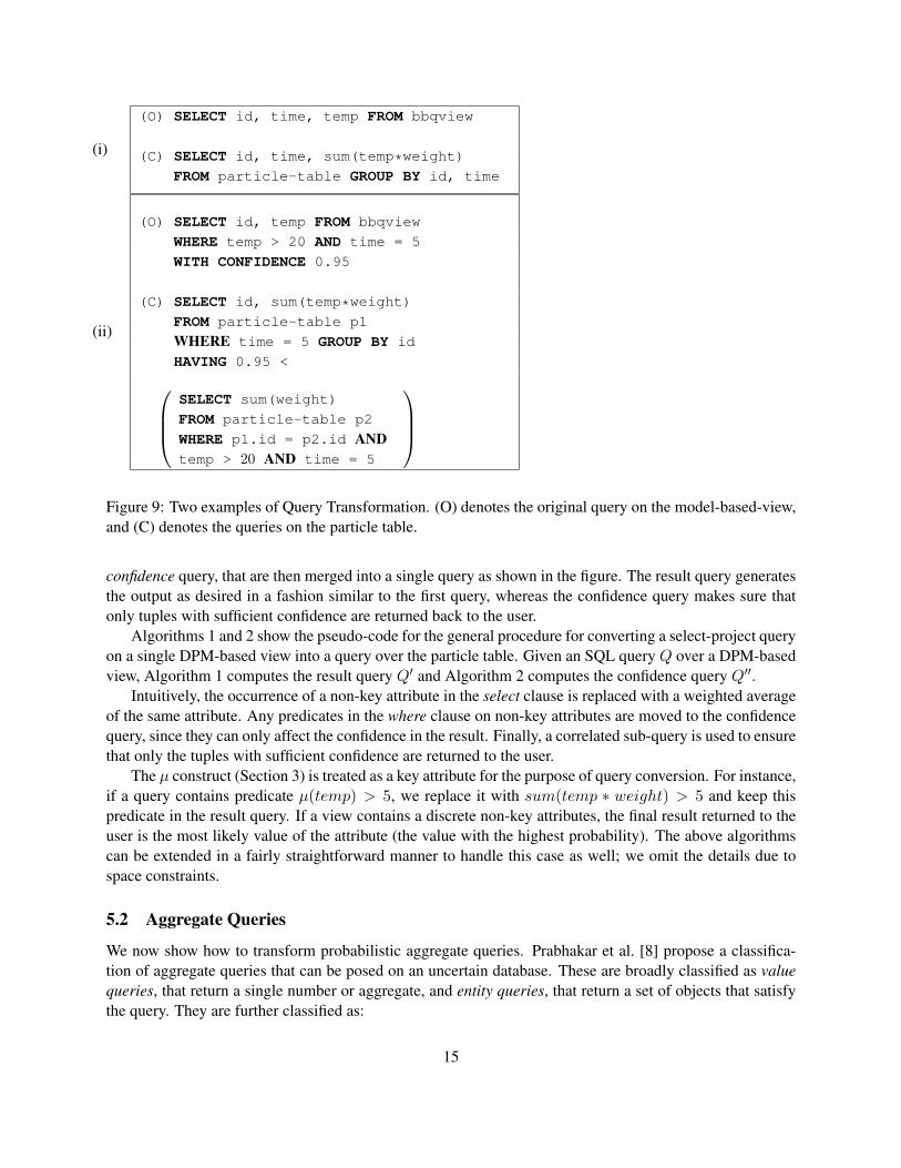
5.1 Select-Project SQL queries

Figure 9 shows two examples of query transformation over this view. The first query simply asks for thetemperatures measured by all sensors. As we discussed in Section 3, if the final result attributes in a queryare probabilistic, the expected values are returned instead. As shown in Figure 9, the corresponding queryover the particle table simply groups the particles by the key attributes and returns a weighted average of thetemperature attribute.

Algorithm 2 Constructing the confidence queryRequire: User SQL Query (Q) on the model based view.

1: Construct Query Q′′ such that,2: SELECT clause of Q′′← sum(weight)3: FROM clause of Q′′← particle-table p24: WHERE clause of Q′′←WHERE clause of Q5: Add ‘p1.key = p2.key’ predicates to WHERE clause of Q′

The second query specifies a predicate over a probabilistic attribute and a confidence value that specifiesthe minimum confidence required in the result tuples (a default confidence value is assumed if the userdoesn’t specify one). In such a case, the query transformer constructs two queries, a result query and a

14

(i)

(O) SELECT id, time, temp FROM bbqview

(C) SELECT id, time, sum(temp*weight)

FROM particle-table GROUP BY id, time

(ii)

(O) SELECT id, temp FROM bbqview

WHERE temp > 20 AND time = 5

WITH CONFIDENCE 0.95

(C) SELECT id, sum(temp*weight)

FROM particle-table p1

WHERE time = 5 GROUP BY id

HAVING 0.95 <SELECT sum(weight)

FROM particle-table p2

WHERE p1.id = p2.id ANDtemp > 20 AND time = 5

Figure 9: Two examples of Query Transformation. (O) denotes the original query on the model-based-view,and (C) denotes the queries on the particle table.

confidence query, that are then merged into a single query as shown in the figure. The result query generatesthe output as desired in a fashion similar to the first query, whereas the confidence query makes sure thatonly tuples with sufficient confidence are returned back to the user.

Algorithms 1 and 2 show the pseudo-code for the general procedure for converting a select-project queryon a single DPM-based view into a query over the particle table. Given an SQL query Q over a DPM-basedview, Algorithm 1 computes the result query Q′ and Algorithm 2 computes the confidence query Q′′.

Intuitively, the occurrence of a non-key attribute in the select clause is replaced with a weighted averageof the same attribute. Any predicates in the where clause on non-key attributes are moved to the confidencequery, since they can only affect the confidence in the result. Finally, a correlated sub-query is used to ensurethat only the tuples with sufficient confidence are returned to the user.

The µ construct (Section 3) is treated as a key attribute for the purpose of query conversion. For instance,if a query contains predicate µ(temp) > 5, we replace it with sum(temp ∗ weight) > 5 and keep thispredicate in the result query. If a view contains a discrete non-key attributes, the final result returned to theuser is the most likely value of the attribute (the value with the highest probability). The above algorithmscan be extended in a fairly straightforward manner to handle this case as well; we omit the details due tospace constraints.

5.2 Aggregate Queries

We now show how to transform probabilistic aggregate queries. Prabhakar et al. [8] propose a classifica-tion of aggregate queries that can be posed on an uncertain database. These are broadly classified as valuequeries, that return a single number or aggregate, and entity queries, that return a set of objects that satisfythe query. They are further classified as:

15

• Aggregate Value queries

(1) Probabilistic Sum, Avg Query (VSumQ, VAvgQ)(2) Probabilistic Min, Max Query (VMinQ, VMaxQ)• Aggregate Entity queries

(1) Probabilistic Range Query (ERQ)(2) Probabilistic Min, Max Query (EMinQ, EMaxQ)(3) Probabilistic Nearest Neighbor Query (ENNQ)

We illustrate our conversion routines for each type of query mentioned above.

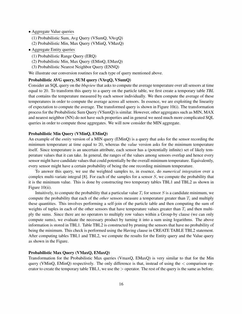
Probabilistic AVG query, SUM query (VAvgQ, VSumQ)Consider an SQL query on the bbqview that asks to compute the average temperature over all sensors at timeequal to 20. To transform this query to a query on the particle table, we first create a temporary table TBLthat contains the temperature measured by each sensor individually. We then compute the average of thesetemperatures in order to compute the average across all sensors. In essence, we are exploiting the linearityof expectation to compute the average. The transformed query is shown in Figure 10(i). The transformationprocess for the Probabilistic Sum Query (VSumQ) is similar. However, other aggregates such as MIN, MAXand nearest neighbor (NN) do not have such properties and in general we need much more complicated SQLqueries in order to compute those aggregates. We will now consider the MIN aggregate.

Probabilistic Min Query (VMinQ, EMinQ)An example of the entity version of a MIN query (EMinQ) is a query that asks for the sensor recording theminimum temperature at time equal to 20, whereas the value version asks for the minimum temperatureitself. Since temperature is an uncertain attribute, each sensor has a (potentially infinite) set of likely tem-perature values that it can take. In general, the ranges of the values among sensors overlap and hence everysensor might have candidate values that could potentially be the overall minimum temperature. Equivalently,every sensor might have a certain probability of being the one recording minimum temperature.

To answer this query, we use the weighted samples to, in essence, do numerical integration over acomplex multi-variate integral [8]. For each of the samples for a sensor S, we compute the probability thatit is the minimum value. This is done by constructing two temporary tables TBL1 and TBL2 as shown inFigure 10(ii).

Intuitively, to compute the probability that a particular value Ti for sensor S is a candidate minimum, wecompute the probability that each of the other sensors measure a temperature greater than Ti and multiplythese quantities. This involves performing a self-join of the particle table and then computing the sum ofweights of tuples in each of the other sensors that have temperature values greater than Ti and then multi-ply the sums. Since there are no operators to multiply row values within a Group-by clause (we can onlycompute sums), we evaluate the necessary product by turning it into a sum using logarithms. The aboveinformation is stored in TBL1. Table TBL2 is constructed by pruning the sensors that have no probability ofbeing the minimum. This check is performed using the Having clause in CREATE TABLE TBL2 statement.After computing tables TBL1 and TBL2, we compute the results for the Entity query and the Value queryas shown in the Figure.

Probabilistic Max Query (VMaxQ, EMaxQ)Transformation for the Probabilistic Max queries (VmaxQ, EMaxQ) is very similar to that for the Minquery (VMinQ, EMinQ) respectively. The only difference is that, instead of using the < comparison op-erator to create the temporary table TBL1, we use the> operator. The rest of the query is the same as before.

16

WITH TBL AS

SELECT id, sum(weight*temp)

FROM particles WHERE time = 20GROUP BY id

SELECT avg(temp) FROM TBL T;

(i) Transforming the AVG query (Original Query not shown)

WITH TBL1 AS (SELECT p.id AS pid, p.temp AS temp,

p.weight AS weight, q.id AS qid

log(sum(q.weight)) AS logsum

FROM particles p, particles q

WHERE pid != qid AND p.temp < q.temp

AND p.time = 20 AND q.time = 20GROUP BY p.id, p.temp, p.weight,q.id

)WITH TBL2 AS (SELECT pid, temp, weight,

exp(sum(logsum)) AS probability

FROM TBL1

GROUP BY pid, temp

HAVING Count(*)= (SELECT COUNT(distinct id)

FROM particles) - 1)SELECT sum(probability*weight*temp)

FROM TBL2;(a) VMinQ

SELECT pid, sum(probability*weight)

FROM TBL2 GROUP BY pid;

(b) EMinQ

(ii) Transformation of MIN query (Original Query not shown)

Figure 10: Examples of Aggregate Query Transformation.

Probabilistic Range Query (ERQ)Consider an SQL query that determines the sensors that measure temperatures between a given range[Tl, Tu]. As temperature is an uncertain attribute, every sensor will have a non-zero probability of measuringtemperature in the above range. Therefore, to execute this query, we need to integrate the temperature prob-ability distribution of each sensor in the given range [Tl, Tu] to compute the necessary probability values.Since, we have a sample based representation of the temperature probability distribution, the integration canbe easily performed by just computing the sum of weights. The transformed query on the particle table isshown in Figure 11(i).

Probabilistic Nearest Neighbor Query ENNQ

17

SELECT id, sum(weight) FROM particles

WHERE time = t and temp > Tl and temp < Tu

GROUP BY id, time

(i) Transformation of the Probabilistic Range query (Original query not shown)

WITH TBL1 AS (SELECT p.id AS pid, p.temp AS temp,

p.weight AS weight, q.id AS qid

log(sum(q.weight)) AS logsum

FROM particles p, particles q

WHERE pid != qid AND abs(p.temp-r) < (q.temp-r)

AND p.time = 20 AND q.time = 20GROUP BY p.id, p.temp, p.weight,q.id

)WITH TBL2 AS (SELECT pid, temp, weight,

exp(sum(logsum)) AS probability

FROM TBL1

GROUP BY pid, temp

HAVING Count(*)= (SELECT COUNT(distinct id)

FROM particles) - 1)SELECT sum(probability*weight*temp)

FROM TBL2;(a) VMinQ

SELECT pid, sum(probability*weight)

FROM TBL2 GROUP BY pid;

(b) EMinQ

(ii) Transformation of the Nearest Neighbor query (Original Query not shown)

Figure 11: More examples of Aggregate Query conversion

An example of the nearest neighbor query is the following. Report the sensor(s) that measures temperatureclosest to a given value r at time t. In essence, we need to determine the sensor i such that ∀j 6=i|Ti − r| <|Tj − r|. Effectively, we are determining the sensor with the minimum value of |T − q|. We can thereforeexecute the Nearest neighbour query just as the Min query, only with a different expression to minimize.The transformed query is shown in Figure 11(ii).

6 Update Manager

The update manager is in charge of keeping the particle table updated and consistent with the incoming datastream. We use a sequential Monte Carlo technique called particle filtering for this purpose. We present abrief overview of this inference technique next.

18

6.1 Particle Filters

Particle filtering [14] is a well known sequential Monte Carlo algorithm for performing state estimation inDPMs, and has been shown to be effective in a wide variety of scenarios. In short, the algorithm computesand constantly maintains sets of particles to describe the historical and present states of the model. Asdiscussed in Section 3, this is essentially the internal representation that our system uses to maintain theDPM-based views.

There are five components to the particle filtering technique: initialization, prediction, filtering, re-sampling, and smoothing. Algorithms 3, 4 and 5 show the pseudo-code for some of these routines. Weillustrate thse routines using the BBQ DPM(Figure 3(i)).

Initialization: At the beginning of the process, an initial set of particles is created by randomly samplingfrom the prior distributions on the attributes.

Prediction: The prediction step is invoked to advance time. During this step, the state at time t + 1 isestimated using the state at time t. This is done using the conditional probability distributions associ-ated with the model. More specifically, for each existing particle at time t, a new particle for time t + 1is created by sampling from an appropriate CPD. Let (T i

t , Hit) denote the ith particle at time t for our

model. The corresponding particle at time t+1, (T it+1, H

it+1), is created by sampling from the distributions

p(Tt+1|Tt, hourt+1) and p(Ht+1|Ht, hourt+1) where hourt+1 is the hour at time t+ 1.(Section 2.3)

Filtering: The filtering procedure involves using the updates that arrive at time t + 1 to update the stateestimate at time t + 1. First, each new particle is assigned a weight based on the values of the observedvariables at time t + 1. Particles closer to the observed values receive higher weights compared to theparticles that are further from the observed values. These weights are computed using the CPDs of theobserved nodes. For our running example, the weights are assigned to the predicted particles based onthe CPD of the observed node Mt, p(Mt|Ht). This step is typically integrated with the prediction step(Algorithm 3). At the end of the step, the weights are normalized so they sum up to 1.

Re-sampling: One of the critical problems with the particle filtering technique is that it may degenerate tothe case where a single particle has all the weight. This is handled through a re-sampling step, where the setof particles created in the filtering step are re-sampled to generate a new set of particles. The re-samplingstep creates a new set of particles, all with the same weight, thus taking care of the degeneracy. Note thatthe same particle may be repeated multiple times in the resulting set of particles. This is not a problem asthe next prediction step will generate different new particles from these identical particles.

Smoothing: This routine uses the current state distribution to “correct” the state at previous times. Weillustrate this with an example. Consider a scenario where the temperature being modeled changes suddenly.However, the first reading that contains this change may not affect the inferred temperature because of thenoise in the process. Over time as new readings arrive all confirming the change, the inference processbecomes more sure of the change in temperature. Intuitively speaking, the earlier change that was attributedto the noise, should now be re-attributed to an actual change in the temperature. This is done using thesmoothing procedure which recomputes the weights of the particles at earlier times. In theory, the changeshould be propagated all the way back to time = 0. However the effect typically diminishes after a fewsteps, and we only update the distribution of those steps that are atmost L time units away (where L is calledthe smoothing lag). The pseudo-code for smoothing is shown in Algorithm 4.The Smoothing step is present in order to reduce the variance in the filtering output. However, it is a veryexpensive operation - O(N2L) where N is the number of particles; and hence not performed at every timestep. This offers trade-off between accuracy and performance where in we can control the smoothing oper-

19

Algorithm 3 Prediction and FilteringRequire: Particles at time t; Observations obs made at time t+ 1.

1: for each particle pit at time t do

2: Create a partial particle, pit+1, for time t+ 1

3: for every hidden node Xjt+1 in the time slice for t+ 1 in the topological order do

4: Let Pa(Xjt+1) denote the parents of Xj

t+1

5: Let v denote the values of Pa(Xj) (from pit or from pi

t+1 constructed so far)6: Sample a value for Xj

t+1 from p(Xjt+1|Pa(X

jt ) = v).

7: Add the new sampled value to pit+1.

8: Set weight of new particle, wit+1 = 1.

9: for every observed node Y jt+1 do

10: wit+1 = wi

t+1 p(Yjt+1 = obsj |Pa(Y j

t+1))

Algorithm 4 SmoothingRequire: Smoothing lag L; Particles from time T to T − L

1: for time t = T to T-L do2: for each particle pi

t at time t do

3: wit = wi

t

∑Nj=1w

jt+1

p(Xjt+1|Xi

t)PNk=1 wkt p(Xj

t+1|Xkt )

Algorithm 5 Update Manager1: Initialize the particle table by sampling from the prior distributions of the hidden nodes in the first slice

of DPM.2: for each time instant t do3: Predict a new set of particles for time t+ 1 from the old particle set at time t.4: if New data obst in data stream at time t then5: Filter particles based on obst.6: Resample new particles.7: Smooth the particles at previous times (up to t− L) using obst.

ation and its lag in order to obtain necessary bounds. But in many models, Smoothing does not significantlyimprove upon the results (reduce variance) of the filtering step and in those cases filtering alone guaranteessufficient modeling accuracy with good performance.The update manager repeatedly invokes the routines described above to keep the particle table updated asnew data tuples arrive. The pseudo-code for the update manager is shown in Algorithm 5.

7 Learning

7.1 Maximum Likelihood Estimation

Maximum likelihood estimation (MLE) is a popular statistical method used to learn parameters of the un-derlying probability distribution from a given data set. Suppose that we have a sample of data X1, . . . , Xn

and we want to infer the distribution it came from. A common assumption made is that the data is inde-pendent and identically distributed (iid) from a parametric distribution with unknown parameters. We use

20

the MLE technique to estimate the unknown parameters. If the probability distribution to be determined hasparametric form f and is parametrized by θ, then we try to maximize the likelihood function, which is givenby.

L(θ) = f(x1, x2, x3 . . . , xn|θ)

Since the data are iid, we can simplify the above expression as follows.

L(θ) = πni f(xi|θ)

log(L(θ)) =n∑i

log(f(xi|θ))

We then determine the value of θ that maximizes the above log likelihood function. A simple illustration ofthe above method for determining parameters of the Gaussian distribution is shown below.

p(xi|µ, σ) = N(µ, σ) =1√2πσ

e−(xi−µ)2

σ2

Hence, log(L(µ, σ)) =n∑

i=1

(−log(σ)− (xi − µ)2

σ2

)Optimizing the above expression with respect to µ and σ independently gives us the following values.

µ =n∑

i=1

xi/n

σ =n∑

i=1

(xi − µ)2/n

7.2 Learning CPDs

For the applications in our system, we have to learn conditional probability distributions of the formP [X|Pa(X)].In order to learn CPDs, we initially learn the joint distribution P [X,Pa(X)] using MLE and then obtainthe expression for the conditional distribution using Baye’s theorem. We continue to illustrate using theGaussian example. Let us suppose we want to compute P [X|Y ] from P [X,Y ]. Let Z denote the randomvariable [X,Y ].

Let the vector z = [XT , Y T ]T be distributed according to:

z =[

xy

]∼ N

([ab

],

[A CCT B

])Then, the conditional distribution Pr[X|Y ] (which is computed using Baye’s rule) is given by

P [X|Y] = N(a + cB−1(y − b),A−CB−1CT)

8 Implementation Details

In this section, we briefly discuss the implementation details of our system. We have built a prototype of oursystem using Java, and we use the open source Apache Derby (Java embedded database system) [3] to store

21

(i) SELECT first.OID, second.OID, first.time

FROM kfview first, kfview second

WHERE (first.time = second.time)

AND (|first.µ(x) - second.µ(x)| < δ)

AND (|first.µ(y) - second.µ(y)| < δ)

(ii) SELECT kfview.x, kfview.y

FROM kfview WHERE kfview.OID = 4

Figure 12: Queries used in the experiments: (i) An intersection query, and (ii) a trajectory query on theKFM-based view for moving objects;

the particle tables. Our prototype implementation is currently an application level software that lies abovethe Derby abstraction layer. The application accesses the particle tables using JDBC calls. In addition, wecache the particles that belong to the last L time steps (smoothing lag, Section 6.1) in memory for efficientaccess; the particles are written to the database in background. We are currently working on moving theentire implementation inside Derby. The experiments we present in the next section were conducted on aLinux machine with 1.8 GHz Intel Pentium-IV processor with 512 MB of memory.

Perhaps the single most important challenge we faced in our implementation was handling the manydifferent possible types of node variables and their associated CPDs. Nodes in a DPM can be continuousor discrete (with a variety of domains). A node may have any number of discrete or continuous parentattributes, and the CPD itself may be a known parametric function or may be non-parametric. Hence theimplementation needs to be generic in order to support the various forms. Also, we need to provide flexibilityto the user to easily augment the system, for instance, by adding a new CPD that is not currently supportedbut is suitable for her application.

Extensible CPD APIWe abstract all the details specific to CPDs inside a CPD object and export only the generic functions thatare necessary for the higher level learning and inference procedures. To add a new probability distributionfor use as a CPD, the implementor must provide the following functions:• public Object getSampleFromCPD(ArrayList pVals):

This function produces a new sample value for the node given the value of its parents (supplied in theArrayList).

• double getProbability(double val, ArrayList pVals):This function returns the probability that the node variable takes the value val, given its parents values (asspecified in pVals).

• public void addSample(double val, ArrayList pVals): This function adds a new data sample to therepository of samples used to learn this particular CPD.

• public void computeParams(): This function, invoked after all the training samples are added, is usedto “learn” the parameters of the CPD.

9 System Evaluation

In this section we present results from the experimental evaluation of our prototype implementation. Thesalient points of our study can be summarized as follows:

22

1. Necessity: Using dynamic probabilistic models is a must to deal with erroneous and incomplete real-world data streams.

2. Accuracy: Error (MSE) obtained in the inference process follows theoretically expected 1/N be-havior [14] where N is the number of particles. With as few as 100 particles, the error percentageobtained on a real dataset was less that 1%.

3. Efficiency: Inference times required by our system, even with large number of particles (about 1000)is quite small (less than 20ms) and it is hence feasible to use it for online inference in high rate datastreams.

9.1 Experimental setup

We use the following two datasets for our evaluation.

Dataset I: Moving ObjectsWith an increasing amount of location data (e.g. GPS data) available today and the interest in providinglocation-based services using such data, moving objects databases have received much attention in recentyears [37, 42, 8]. We consider a moving objects scenario where a number of point objects are moving aroundin a 2-dimensional space. We assume that each object is fitted with a GPS device that constantly transmits itsposition to a central server. The GPS data may contain noise, and some location updates may be lost in theprocess. We are interested in modeling the above data stream to infer the true locations and the velocitiesof the objects. Lacking a real-world dataset with GPS traces over multiple objects, we instead generatesimulated data with the properties described above. We simulate GPS readings of random trajectories forthese objects. We add a white Gaussian noise with a standard deviation of 2 units to insert noise in the data.In addition, we drop 5% of the readings randomly to model incomplete data and communication failures.

We use the KFM model to process this data and to infer the true locations and velocities (Section 2.2).We perform smoothing operation with a lag of 2. Each moving object is modeled separately using a differ-ent KFM model, but we store the information about all objects in a single table. We use the view creationcommand shown along with the configuration file shown in Figure 7(i) to create these views. The schemaof this view is:

kfview(time, OID, x, y, vx, vy)

Dataset II: Sensor DataThere has been much work recently [12, 34, 8] on managing noisy and incomplete sensor data and inferringuseful information from them. We attempt to use our system to perform similar tasks. We use the publiclyavailable Intel Lab dataset [27] that consists of traces from a 54-node sensor network deployment at theIntel lab in Berkeley. The dataset consists of light, humidity and temperature readings collected in the lab.The readings collected are extremely noisy and in many cases incomplete. Also, several sensors failedmidway through deployment and most of them continued to transmit erroneous values leading to moreerrors. It is also observed the dataset has intra-tuple correlations (temperature and humidity) and inter-tuple correlations across time. In order to decrease acquisition costs for query processing in power awaresensor networks, the efficient strategy [12] is to observe only a few subset of attributes that are easy toacquire, and infer the rest of the attributes from a probabilistic model. In our experiment we attempt toaccurately infer the values of the temperature based on the observed humidity readings using the dynamicprobabilistic model shown in Figure 3(i). We ran a series of processings tasks overs this data.

Step 1: Remove Incorrect Data We first remove incorrect values from the dataset. This involves detection

23

0

20

40

60

80

100

0 0.2 0.4 0.6 0.8 1 1.2

% m

issed

inte

rsec

tions

Delta

Raw GPS dataKalman filter based view

0

20

40

60

80

100

0 100 200 300 400 500 600

Tem

pera

ture

Time

Temperature acquired by SensorWorking/Faulty (DPM-based View)

status = working

status = Faulty 10

15

20

25

30

35

0 400 800 1200 1600 2000

Tem

pera

ture

Time

Temperature recorded by sensorWorking/Faulty (DPM based view)

status = Working

status = Faulty

Figure 13: (i) The % of missed intersections as a function of δ on the raw data and the KFM-based view;(ii) The observed temperatures at a sensor, and the status inferred using an HMM. (iii) Same as (ii) withsimulated faults inserted.

of the failure times of the sensor nodes. We perform this using an HMM-based view based on theHMM model shown in Figure 2(i).

Step 2: Learn DPM Once the incorrect sensor readings are removed, we split the data into training andtesting datasets. The training dataset (data collected for 6 days) is used to learn the conditional prob-ability distributions of the nodes.

Step 3: Inferring Temperature values We then use the humidity readings in the test dataset (data collectedfor 3 days) to infer the temperatures using the BBQ DPM shown in Figure 3(i) by generating bbqview.

Step 4: True Temperature Values In order to evaluate the accuracy of the inferred temperatures, we re-move noise from the observed temperatures using another DPM based view. (The DPM used is similarto a KFM and is not shown). The resulting correct temperatures are compared with the temperaturesinferred from Step 3 to evaluate the accuracy of the inferred temperatures.

9.2 Experimental Results

Applying DPMs to data is criticalDataset I: To show the importance of modeling the data streams, we pose an intersection query over themoving objects database (Figure 12(i)). This query measures the number of intersections between objects,ie., the times at which two particles are closer than a specified distance δ. We execute the same query onthe raw GPS data and compare the number of correct intersections that are measured in both cases. Figure13(i) shows the plot comparing the percentage of missed intersections in the raw data and the KFM-basedview. As we can see, a large number of the intersections are missed while executing the query on the rawdata, especially for smaller values of δ. This is both because of the missing data and the noise in the data.The KFM-based view, on the other hand, is able to capture most of the real intersections in the data.Dataset II: Figures 13(ii), (iii) show the temperature values that were measured by the sensors and thosereadings that were marked as incorrect by the HMM-based view. As we can see from Figure 13(ii), thereare several incorrect values after 500 hours (20 days approx), that need to be removed before we can usethem for learning. We also added a few simulated faults in order to further verify that the HMM-based viewcorrectly identifies the faulty readings.

Inference using particle filtering is accurate

24

0

2

4

6

8

10

12

14

16

18

10 100 1000 10000

Mea

n Sq

uare

d Er

ror

Number of particles(log scale)

GPS from KF ViewRaw GPS data

Temperature from DPM View

0.001

0.01

0.1

1

10

100

0 100 200 300 400 500 600 700 800 900 1000

Tim

e pe

r Inf

eren

ce S

tep(

sec)

Number of particles

L = 4

L = 2

L = 1

L=0, filtering

Time = 2s

Time = 20ms

0

10

20

30

40

50

60

10 100 1000

Tim

e pe

r inf

eren

ce s

tep

(milli

seco

nd)

Number of particles (log scale)

Particle Filtering(Our system)Analytical Filtering(AKF)

(i) (ii) (iii)

Figure 14: (i) Plot of mean-squared error vs number of particles for both kfview (Dataset I) and bbqview(Dataset II). Mean squared error falls off as (1/N) (ii) Graph shows time taken for one inference step atvarious smoothing lags. (iii) The update times for particle filtering are comparable to those for an analyticaltechnique.

With this set of experiments, we show that the particle filtering algorithm accurately determines the hiddenstate of the system being modeled.Dataset I: We execute the trajectory query shown in Figure 12(ii), that returns the path traced by object4, on the raw data and on the KFM-based view. The accuracy of the result is measured by computing thedeviation of the path from its actual path using the sum-squared error function. We plot the estimate of theerror as a function of the number of particles (N ) in Figure 14(i).Dataset II: We compare the value of temperatures that were inferred by the bbqview (with just filtering, nosmoothing) to the true temperature values generated in Step 4. We compute a mean square error estimateand plot the mean squared error as a function of the number of particles. We obtain the graph shown infigure 14(i).

From the plots, we can see that the error in the KFM-based views for GPS datasets is much less than thatin the raw data. (Error in raw data is indicated by the straight line.) We also verify that the error decreases asthe number of particles used increases. For low values of N , the error reduces drastically in the beginning,however, for higher values of N (more than 100 particles), it remains fairly constant. Both the error graphsfollow the theoretically estimated (1/N) graph which validates our experiments. For the temperature data(dataset II), the mean square error obtained on the test data with just Filtering alone is less than 0.25 units(≤1% error) when just 100 particles are used.

Inference using particle filtering is efficientNext, we provide details regarding the performance of our system.Learning: Given data to be modeled and a DPM, time is initially spent for learning the CPDs. Learningthe CPDs for the Temperature and Humidity nodes in the BBQ DPM from about 430000 records (each ofdimension 3) took about 7.5 seconds.Inference: After the CPDs are learnt and we receive data continuously, time is spent on performing theInference procedure. The inference procedure, performed at each time instant, results in addition of severalnew rows and modification of already existing rows, if smoothing is used. We measure the time taken forone inference step as a function of the number of particles. We carry out this experiment for different valuesof the smoothing lag parameter, L = 0, 1, 2, 4. The results obtained are shown in Figure 14(ii). We findthat the execution time increases linearly with increase in the number of particles (as y-axis is in log scale,this cannot be explicitly seen). If we perform only filtering, the inference time is very small; we process

25

more than 1000 particles in just 20ms. However, if we continuously perform smoothing, the time taken forinference increases drastically as shown in the graph. However, even with a smoothing lag of 4 time steps,we can process 100 particles in less than 100ms (reasonable for most common streams). As the accuracygraph shows in Figure 14(i), this may be enough to achieve sufficient accuracy. We are considering “lazy”smoothing strategies where we perform smoothing ocassionally (not at every time step) and only when it isessential.Comparison to Analytical Filtering: As there are no other systems that perform tasks similar to our sys-tem, we implemented an analytical solution for Kalman Filters (called AKF). We compare the performanceof our particle filtering inference algorithm against AKF. In AKF, particles are directly sampled using themathematical equations for the Kalman filter [43] and are inserted into the database in order to obtain acommon ground for comparison. Note that even for AKF, we have to generate the samples in order to ex-ecute queries against the output of the model. We compare the time taken by our system (the KFM-basedview for Dataset I) against AKF. For both the systems, we do not perform the Smoothing procedure. Figure14(iii) shows the execution times for a single inference step as a function of the number of particles. As ex-pected, the Kalman filter implementation using analytical formulas takes less time than the particle filteringalgorithm. However the difference between the two is not significant except when the number of particles isvery large. We would also like to note that our prototype implementation is not fine-tuned for performance,and we expect that a more careful implementation will reduce the time taken by our implementation evenfurther.

10 Related Work

Bayesian Networks and Dynamic Probabilistic Models: Bayesian networks have a long and rich historyacross a wide variety of research disciplines, and numerous books have been written addressing several as-pects of such models (e.g. [35, 22]). Dynamic probabilistic models (sometimes called dynamic Bayesiannetworks, or dynamic probabilistic networks), a relatively newer and less well-established concept, allowreasoning about the temporal dimension as well, and are used extensively for modeling complex stochasticprocesses [16, 33, 30]. In recent years, they have been seen as the tool to unify similar concepts in seem-ingly disparate domains such as probabilistic expert systems, statistical physics, image analysis, geneticsand so on [41, 18]. For instance, both HMMs and Kalman filters, perhaps the most common examples ofsuch models, were developed independently in engineering and speech recognition communities, and theirsimilarities to graphical models have been observed fairly recently [40, 25]. Over the years, several generalpurpose toolkits have been developed that support Bayesian networks, and in some cases, dynamic Bayesiannetworks (e.g. [32, 20]). However, to the best of our knowledge, ours is the first work that proposes to di-rectly implement arbitrary dynamic probabilistic models inside databases thereby making it easier to useDPMs, and also increasing the functionality and appeal of relational database systems. Probabilistic rela-tional models [17] are a generalization of Bayesian networks to learning probabilistic models of the datapresent in relational tables. More recently, dynamic probabilistic relational probabilistic models have alsobeen considered in the machine learning community [38]. This work is also complementary to our approachhere.Probabilistic Databases: In recent years, we have seen a renewed interest in the area of probabilisticdatabases, fueled primarily by a large increase in the amount of real-world data that is inherently noisy,incomplete and uncertain (e.g., [24, 4, 11, 44, 39]). Several research efforts are underway to build systemsto manage uncertain data (e.g. MYSTIQ [11], Trio [44], ORION [8], ConQuer [2]). As we discussed inSection 3, views based on dynamic probabilistic models are naturally probabilistic, and we plan to use the

26

techniques developed in the probabilistic databases research, especially query languages and semantics, inour future work.Data Streams & Sensor Networks: Many data stream management systems have been proposed for real-time processing of continuously generated data by sensor networks [6, 7, 5, 31]. The main focus of thatwork has been on efficient evaluation of large number of continuous queries over high-rate streaming data.Our work is complementary to this work; it focuses on efficiently modeling streaming data so that the queryresults can be more meaningful and useful to the user.

Sensor networks have been a very active area of research in recent years (see [1] for a survey), andthere is a large body of work on data collection from sensor networks that applies higher-level techniquesto sensor network data processing. TinyDB and Cougar [45, 28] provide declarative interfaces to acquiringdata from sensor networks. Several systems propose to use probabilistic modeling techniques to answerqueries over sensor networks [21, 12, 10], though these have typically used specific models rather than ageneralized implementation in an existing relational database. Finally, as discussed in Section 3, our systemgeneralizes and significantly enriches the abstraction of model-based views that was originally proposed inthe MauveDB system [13].

11 Conclusions

Advances in miniaturization technology and networking have resulted in a rapid increase in the number oflarge-scale deployments of measurement infrastructures that continuously generate tremendous volumes ofpriceless data. In this paper, we presented an approach to build an extensible database system that enablesusers to apply general purpose dynamic probabilistic models to such data in real-time, thus significantly en-riching the functionality and the appeal of databases for managing such data. We provide intuitive interfacesto declaratively specify the models to be applied, and to query the output of the application of such modelsto data streams. We use particle filtering to perform the inference tasks, and we show how this also enablesefficient query execution over DPM-based views. The techniques we develop for representing and queryingprobabilistic tables using particles are of independent interest to the probabilistic database community aswell. Our experimental evaluation over a prototype implementation illustrates the advantages of enablingreal-time application of dynamic probabilistic models to streaming data.

References

[1] I.F. Akyildiz, W. Su, Y. Sankarasubramaniam, and E. Cayirci. Wireless sensor networks: a survey.Computer Networks, 38, 2002.

[2] Periklis Andritsos, Ariel Fuxman, and Renee J. Miller. Clean answers over dirty databases. In ICDE,2006.

[3] The Apache Derby Project. Web Site. http://db.apache.org/derby/.[4] D. Barbara, H. Garcia-Molina, and D. Porter. The management of probabilistic data. IEEE TKDE,

4(5):487–502, 1992.[5] D. Carney. Monitoring streams - a new class of data management applications. In VLDB, 2002.[6] Sirish Chandrasekaran. TelegraphCQ: Continuous dataflow processing for an uncertain world. In

CIDR, 2003.[7] Jianjun Chen, David DeWitt, Feng Tian, and Yuan Wang. NiagaraCQ: A scalable continuous query

system for internet databases. In SIGMOD, 2000.

27

[8] R. Cheng, D. V. Kalashnikov, and S. Prabhakar. Evaluating probabilistic queries over imprecise data.In SIGMOD, 2003.

[9] Tanzeem Choudhury, Matthai Philipose, Danny Wyatt, and Jonathan Lester. Towards activitydatabases: Using sensors and statistical models to summarize people’s lives. IEEE Data Eng. Bull.,29(1):49–58, 2006.

[10] M. Chu, H. Haussecker, and F. Zhao. Scalable information-driven sensor querying and routing for adhoc heterogeneous sensor networks. In Intl Journal of High Performance Computing Applications,2002.

[11] Nilesh N. Dalvi and Dan Suciu. Efficient query evaluation on probabilistic databases. In VLDB, 2004.[12] Amol Deshpande, Carlos Guestrin, Sam Madden, Joe Hellerstein, and Wei Hong. Model-driven data

acquisition in sensor networks. In VLDB, 2004.[13] Amol Deshpande and Samuel Madden. MauveDB: supporting model-based user views in database

systems. In SIGMOD Conference, pages 73–84, 2006.[14] Arnaud Doucet, Nando de Freitas, and Neil Gordon. Sequential Monte Carlo methods in practice.

Springer, 2005.[15] R. Durbin, S. R. Eddy, A. Krogh, and G. Mitchison. Biological Sequence Analysis: Probabilistic

Models of Proteins and Nucleic Acids. Cambridge Univ Press, 1999.[16] N. Friedman, K. Murphy, and S. Russell. Learning the structure of dynamic probabilistic networks. In

UAI, 1998.[17] Lise Getoor. Learning Statistical Models from Relat- ional Data. PhD thesis, Stanford University,

2001.[18] Zoubin Ghahramani. Learning dynamic Bayesian networks. Lecture Notes in Computer Science, 1387,

1998.[19] E. Hoke, J. Sun, and C. Faloutsos. Intemon: Intelligent system monitoring on large clusters. In VLDB,

2006.[20] S. Hjsgaard and C. Dethlefsen. The grbase package for graphical modelling in R. Technical Report

R-2004-19, Aalborg University, 2004.[21] A. Jain, E. Change, and Y. Wang. Adaptive stream resource management using kalman filters. In

SIGMOD, 2004.[22] Michael I. Jordan. Learning in Graphical Models (ed). MIT Press, 1998.[23] F. Koushanfar, M. Potkonjak, and A. Sangiovanni-Vincentelli. On-line fault detection of sensor mea-

surements. IEEE Sensors, 2003.[24] L. V. S. Lakshmanan, N. Leone, R. Ross, and V. S. Subrahmanian. Probview: a flexible probabilistic

database system. ACM TODS, 22(3), 1997.[25] B.C. Levy, A. Benveniste, and R. Nikoukhah. High-level primitives for recursive maximum likelihood

estimation. IEEE Trans. on Automatic Control, AC-41(8), 1996.[26] D. Lymberopoulos, A.S. Ogale, A. Savvides, and Y. Aloimonos. A sensory grammar for inferring

behaviors in sensor networks. In IPSN, 2006.[27] Sam Madden. Intel lab data, 2004. http://berkeley.intel-research.net/labdata.[28] Samuel Madden, Wei Hong, Joseph M. Hellerstein, and Michael Franklin. TinyDB web page. http:

//telegraph.cs.berkeley.edu/tinydb.[29] A. M. Mainwaring, D. E. Culler, J. Polastre, R. Szewczyk, and J. Anderson. Wireless sensor networks

for habitat monitoring. In WSNA, 2002.[30] V. Mihajlovic and M. Petkovic. Dynamic bayesian networks: A state of the art. University of Twente

Document Repository 2001.

28

[31] Rajeev Motwani. Query processing, resource management, and approximation in a data stream man-agement system. In CIDR, 2003.

[32] Kevin Murphy. The Bayes net toolbox for matlab. Computing Science and Statistics, 33, 2001.[33] Kevin Murphy. Dynamic Bayesian Networks: Representation, Inference and Learnig. PhD thesis, UC

Berkeley, 2002.[34] D. Patterson, L. Liao, D. Fox, and H. Kautz. Inferring high level behavior from low level sensors. In

UBICOMP, 2003.[35] Judea Pearl. Probabilistic Reasoning in Intelligent Systems: Networks of Plausible Inference. Morgan

Kaufmann, 1988.[36] L Rabiner. A tutorial on hidden Markov models and selected applications in speech recognition.

77:257–286, 1989.[37] K. Raptopoulou, M. Vassilakopoulos, and Y. Manolopoulos. Towards quadtree-based moving objects

databases. Lecture Notes in Computer Science, Volume 3255, Jan 2004, 2004.[38] S. Sanghai, P. Domingos, and D. Weld. Dynamic probabilistic relational models. In IJCAI, 2003.[39] P. Sen and A. Deshpande. Representing and querying correlated tuples in probabilistic databases. In

ICDE, 2007.[40] P. Smyth, D. Heckerman, and M. Jordan. Probabilistic independence networks for hidden markov

models. Neural Computation, 9(2):227–269, 1997.[41] Padhraic Smyth. Belief networks, hidden markov models, and markov random fields: a unifying view.

Pattern Recognition Letters, 18(11-13), 1997.[42] Goce Trajcevski, Ouri Wolfson, Klaus Hinrichs, and Sam Chamberlain. Managing uncertainty in

moving objects databases. ACM Trans. Database Syst., 29(3):463–507, 2004.[43] Greg Welch and Gary Bishop. An introduction to the Kalman filter. http://www.cs.unc.edu/

˜welch/kalman/kalmanIntro.html, 2002.[44] J. Widom. Trio: A system for integrated management of data, accuracy, and lineage. In CIDR, 2005.[45] Y. Yao and J. Gehrke. Query processing in sensor networks. In CIDR, 2003.[46] Jie Ying. A hidden markov model-based algorithm for fault diagnosis with partial and imperfect tests.

IEEE Trans. on Systems, Man, and Cybernetics, Part C, 2000.

29