Online Asymmetric Active Learning with Imbalanced Data

Xiaoxuan Zhang, Tianbao Yang, Padmini SrinivasanDepartment of Computer ScienceThe University of Iowa, IA 52242

{xiaoxuan-zhang, tianbao-yang, padmini-srinivasan}@uiowa.edu

ABSTRACTThis paper considers online learning with imbalanced stream-ing data under a query budget, where the act of queryingfor labels is constrained to a budget limit. We study dif-ferent active querying strategies for classification. In par-ticular, we propose an asymmetric active querying strategythat assigns different probabilities for query to examples pre-dicted as positive and negative. To corroborate the proposedasymmetric query model, we provide a theoretical analysison a weighted mistake bound. We conduct extensive eval-uations of the proposed asymmetric active querying strat-egy in comparison with several baseline querying strategiesand with previous online learning algorithms for imbalanceddata. In particular, we perform two types of evaluations ac-cording to which examples appear as “positive”/ “negative”.In push evaluation only the positive predictions given to theuser are taken into account; in push and query evaluationthe decision to query is also considered for evaluation. Thepush and query evaluation strategy is particularly suitedfor a recommendation setting because the items selected forquerying for labels may go to the end-user to enable cus-tomization and personalization. These would not be shownany differently to the end-user compared to recommendedcontent (i.e., the examples predicated as positive). Addi-tionally, given our interest in imbalanced data we measureF -score instead of accuracy that is traditionally consideredby online classification algorithms. We also compare thequerying strategies on five classification tasks from differ-ent domains, and show that the probabilistic query strategyachieves higher F -scores on both types of evaluation than de-terministic strategy, especially when the budget is small, andthe asymmetric query model further improves performance.When compared to the state-of-the-art cost-sensitive onlinelearning algorithm under a budget, our online classificationalgorithm with asymmetric querying achieves a higher F -score on four of the five tasks, especially on the push evalu-ation.

Permission to make digital or hard copies of all or part of this work for personal orclassroom use is granted without fee provided that copies are not made or distributedfor profit or commercial advantage and that copies bear this notice and the full cita-tion on the first page. Copyrights for components of this work owned by others thanACM must be honored. Abstracting with credit is permitted. To copy otherwise, or re-publish, to post on servers or to redistribute to lists, requires prior specific permissionand/or a fee. Request permissions from permissions@acm.org.KDD ’16, August 13-17, 2016, San Francisco, CA, USAc⃝ 2016 ACM. ISBN 978-1-4503-4232-2/16/08. . . $15.00

DOI: http://dx.doi.org/10.1145/2939672.2939854

KeywordsOnline Learning; Query Budget; Imbalanced Data; F-score

1. INTRODUCTIONTraditional batch classification algorithms that have been

broadly applied in various data mining domains, such asdocument filtering [29], news classification [23], spam detec-tion [2], and opinion mining [25], are challenged by appli-cations characterized by large-scale, streaming data as forinstance in web mining applications. Large amounts of dataare continually generated by the web such as through socialmedia and news. These datasets are often also highly imbal-anced with respect to classes of interest. A key consequenceof scale is that getting adequate training data becomes nontrivial in effort and costly. To address these problems, westudy online classification algorithms where the act of query-ing for labels is constrained to a budget limit.

Lowering cost is always a goal in algorithms processinglarge-scale and real-time data. In classification, there aretwo major sources of cost. The first is the obvious costincurred due to errors in performance (false positive andfalse negative decisions). The second is the cost of labelingthe data used to initially build or retrain the model overtime. Focusing on the second cost for the moment, labelleddata may be collected in two general ways with cost differ-ences that are both subtle and explicit. We may directlyask the client (end-user) to provide labels. This approach isparticularly useful for personalized recommendation [8, 1].As a consequence, in addition to giving the client the highconfidence positive predictions made by the system we alsoshow instances of low confidence to label. While risky theselow confidence instances are likely to be the most useful forimproving the performance of the classifier. However, overtime the client may become disappointed if the system takesbig risks with too many false positives shown. Therefore, itmakes sense to limit the amount of queries to label sent tothe end-user. In this paper, we tackle this issue in an onlinesetting for streaming data. We aim to maximize the per-formance subject to a budget limit for querying the labels.There are several fold of entangled difficulties: (i) how todecide which examples to query for the true labels given abudget limit; (ii) which performance measure should we tar-get? (iii) how to evaluate the performance of the system?These difficulties become severe in the presence of imbal-anced data. For example, if there are many more negativeexamples than positive examples, treating them equally formaking the query decisions can be sub-optimal. A ‘bad’query may even harm performance. For example, Figure 2

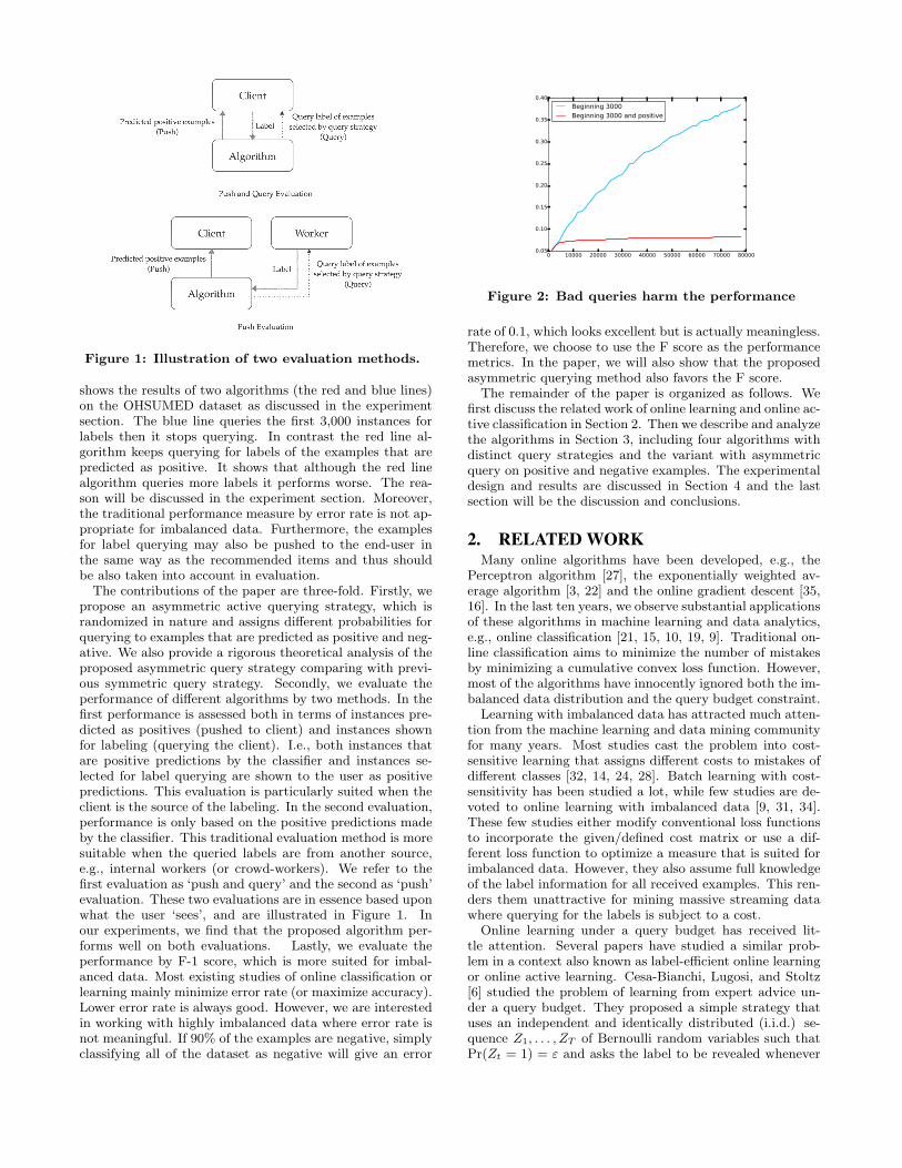
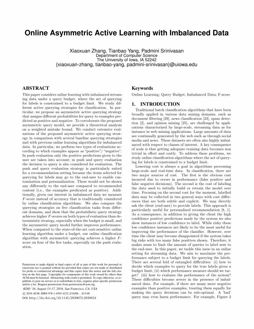
Figure 1: Illustration of two evaluation methods.

shows the results of two algorithms (the red and blue lines)on the OHSUMED dataset as discussed in the experimentsection. The blue line queries the first 3,000 instances forlabels then it stops querying. In contrast the red line al-gorithm keeps querying for labels of the examples that arepredicted as positive. It shows that although the red linealgorithm queries more labels it performs worse. The rea-son will be discussed in the experiment section. Moreover,the traditional performance measure by error rate is not ap-propriate for imbalanced data. Furthermore, the examplesfor label querying may also be pushed to the end-user inthe same way as the recommended items and thus shouldbe also taken into account in evaluation.The contributions of the paper are three-fold. Firstly, we

propose an asymmetric active querying strategy, which israndomized in nature and assigns different probabilities forquerying to examples that are predicted as positive and neg-ative. We also provide a rigorous theoretical analysis of theproposed asymmetric query strategy comparing with previ-ous symmetric query strategy. Secondly, we evaluate theperformance of different algorithms by two methods. In thefirst performance is assessed both in terms of instances pre-dicted as positives (pushed to client) and instances shownfor labeling (querying the client). I.e., both instances thatare positive predictions by the classifier and instances se-lected for label querying are shown to the user as positivepredictions. This evaluation is particularly suited when theclient is the source of the labeling. In the second evaluation,performance is only based on the positive predictions madeby the classifier. This traditional evaluation method is moresuitable when the queried labels are from another source,e.g., internal workers (or crowd-workers). We refer to thefirst evaluation as ‘push and query’ and the second as ‘push’evaluation. These two evaluations are in essence based uponwhat the user ‘sees’, and are illustrated in Figure 1. Inour experiments, we find that the proposed algorithm per-forms well on both evaluations. Lastly, we evaluate theperformance by F-1 score, which is more suited for imbal-anced data. Most existing studies of online classification orlearning mainly minimize error rate (or maximize accuracy).Lower error rate is always good. However, we are interestedin working with highly imbalanced data where error rate isnot meaningful. If 90% of the examples are negative, simplyclassifying all of the dataset as negative will give an error

Figure 2: Bad queries harm the performance

rate of 0.1, which looks excellent but is actually meaningless.Therefore, we choose to use the F score as the performancemetrics. In the paper, we will also show that the proposedasymmetric querying method also favors the F score.

The remainder of the paper is organized as follows. Wefirst discuss the related work of online learning and online ac-tive classification in Section 2. Then we describe and analyzethe algorithms in Section 3, including four algorithms withdistinct query strategies and the variant with asymmetricquery on positive and negative examples. The experimentaldesign and results are discussed in Section 4 and the lastsection will be the discussion and conclusions.

2. RELATED WORKMany online algorithms have been developed, e.g., the

Perceptron algorithm [27], the exponentially weighted av-erage algorithm [3, 22] and the online gradient descent [35,16]. In the last ten years, we observe substantial applicationsof these algorithms in machine learning and data analytics,e.g., online classification [21, 15, 10, 19, 9]. Traditional on-line classification aims to minimize the number of mistakesby minimizing a cumulative convex loss function. However,most of the algorithms have innocently ignored both the im-balanced data distribution and the query budget constraint.

Learning with imbalanced data has attracted much atten-tion from the machine learning and data mining communityfor many years. Most studies cast the problem into cost-sensitive learning that assigns different costs to mistakes ofdifferent classes [32, 14, 24, 28]. Batch learning with cost-sensitivity has been studied a lot, while few studies are de-voted to online learning with imbalanced data [9, 31, 34].These few studies either modify conventional loss functionsto incorporate the given/defined cost matrix or use a dif-ferent loss function to optimize a measure that is suited forimbalanced data. However, they also assume full knowledgeof the label information for all received examples. This ren-ders them unattractive for mining massive streaming datawhere querying for the labels is subject to a cost.

Online learning under a query budget has received lit-tle attention. Several papers have studied a similar prob-lem in a context also known as label-efficient online learningor online active learning. Cesa-Bianchi, Lugosi, and Stoltz[6] studied the problem of learning from expert advice un-der a query budget. They proposed a simple strategy thatuses an independent and identically distributed (i.i.d.) se-quence Z1, . . . , ZT of Bernoulli random variables such thatPr(Zt = 1) = ε and asks the label to be revealed whenever

Zt = 1. The limitation with the pure random query strategyis that it does not differentiate between examples with highconfidence score and low confidence score for classification.Later on, the same authors [7] designed a new strategy ofquery that makes the probability of querying dependent onthe absolute value of the prediction score. This query algo-rithm has also been used in a recent work for cost-sensitiveonline learning [33]. Active learning for querying the labelshas also been considered in different works for different al-gorithms from the perspective of sample complexity [11, 12,4]. [11] analyzed the perceptron-like algorithm under an ac-tive setting and provided a complexity on the number ofqueried labels for achieving a certain generalization perfor-mance. [4, 12] studied online ridge-regression type of algo-rithms for classification for different querying strategies andestablished the sample complexity bound. However, theseworks have not consider the asymmetry between positiveexamples and negative examples for imbalanced data.One of our goals in this paper is to compare different query

strategies for learning with imbalanced data. Moreover, wenote that the symmetric query model where the probabil-ity of querying is independent of the positive/negative de-cision is not well suited for imbalanced data. To under-stand this, consider that the number of positive examples ismuch smaller than the number of negative examples. As aresult, there would be more false positives than false nega-tives. If we assign equal probabilities to these false predictedexamples for querying the label, the algorithm would favorthe negative class more than the positive class, consequen-tially harm the performance. Therefore, we propose a novelasymmetric query model that is demonstrated to be soundin theory and effective in practice as well. Moreover, thecomparison of two different strategies to handle imbalanceddata under a query budget, namely (i) an asymmetric querymodel plus a symmetric updating rule of the proposed al-gorithm, and (ii) an asymmetric updating rule plus a sym-metric query model of a state-of-the-art algorithm [33], alsodemonstrate the proposed algorithm is very useful.

3. ONLINE ACTIVE LEARNING UNDER AQUERY BUDGET

We first introduce some notations. We denote by xt ∈ Rd

the feature vector of the example received at the t-th round,and by yt ∈ {1,−1} the label of xt. Let f(x) denote aprediction function. In the sequel, we will focus on the pre-sentation using the linear model f(x) = w⊤x, while one caneasily generalize it to a non-linear function in a reproducingkernel Hilbert space. Let B > 0 denote a budget limit onthe number of queries.The framework of online classification under a query bud-

get is presented in Algorithm 1. We let wt and Bt denotethe model available before the (t+1)-th round and the bud-get used before the (t + 1)-th round. Initially, the modelis w0 = 0 and B0 = 0. In line 5, the algorithm computespt = w⊤

t−1xt and in line 6 it makes a decision about the bi-nary label of xt by a function yt = Predict(pt) based on pt.The simplest Predict function is yt = sign(pt), i.e., usingthe sign of pt to determine the label. More generally, wecan use a threshold γ and and let yt = sign(pt − γ). Forimbalanced data, we observe that using a threshold alwaysyields better performance. We discuss how to set the valueof γ in the experiment section.

After the binary decision is made, the algorithm entersthe query stage, where it decides whether to query the labeland update the model. When the algorithm reaches thebudget limit, the model will not be updated because queryis not allowed and there are two options for making futurepredictions. The Option I is to use the last updated modeland the Option II is to use the averaged model before theiteration TB when the budget is used up. Many previousstudies have found that the averaged model might give morerobust predictions than the last model [30].

If the remaining budget is not zero, i.e., Bt−1 < B, weuse the output of a query function Zt = Query(pt), whichmight depend on pt and some other parameters, to deter-mine query (Zt = 1) or not (Zt = 0). If Zt is 1, then thealgorithm queries the label of current example denoted byyt ∈ {1,−1} from a source. Then the algorithm proceeds toupdate the model using wt = Upate(wt−1, yt,xt) in line 13.Function Upate depends on what optimization method isemployed and what surrogate loss function is assumed. In-deed, many different updating schemes can be used, includ-ing the margin-based updating rules (e.g., Perceptron [27],online passive-aggressive algorithm [9], confidence-weightedlearning algorithm [13], etc) and online gradient descent up-dates for different types of loss functions [35]. Take thePerceptron for example, wt is updated by

wt = wt−1 + ytxtI(ytft ≤ 0) (1)

where I(v) is an identity function that outputs 1 if v is trueand otherwise outputs zero.

The query model is the key concern in this paper. Be-low we first discuss some baseline models that either arisestraightforwardly or appear in previous work. Then wepresent the proposed query model for imbalanced data.

3.1 Baseline Query ModelsWe discuss several baseline query models below and com-

ment on their deficiencies.

• First Come First Query (referred to as QF). Thisstrategy is simply to query the true labels of the firstB examples and then uses the model learned from thefirst B examples to make predictions for all the follow-ing examples. This strategy is similar to the ϵ-greedystrategy used in bandit learning [20], where the firststage with B examples is devoted to exploration andthe second stage is exploitation.

• Random Query (referred to as QR). This strategy isto use a Bernoulli random variable Zt = Bern(ϵ) thatequals 1 with a probability ϵ to determine whetherto query or not. The random strategy has been usedin predict with expert advices under budget feedbacksetting [5].

• Deterministic prediction dependent Query (referred toas QD). Different from the first two query modelswhere the decision to query does not depend on pt, wecan make the query function dependent on pt. Themotivation is that if pt is closer to zero, meaning thatthe prediction is more uncertain, then we should queryits label for updating the model. This strategy is verysimilar to active learning where uncertain examplesshould be queried first [18]. The deterministic predic-

Algorithm 1 Online Binary Classification Under A QueryBudget

1: Input: budget B2: Initialize w0 = 0, B0 = 03: for t = 1, . . . , T do4: Receive an example xt

5: Compute pt = w⊤t−1xt

6: Make a push decision yt = Predict(pt) ∈ {1,−1}7: if Bt−1 ≥ B then8: Set wt as

Option I: wt = wt−1

Option II: wt =1TB

TB−1∑

t=0

wt

where TB is the smallest number that the budget isused up, i.e., BTB−1 = B.

9: else10: Compute a variable Zt = Query(pt) ∈ {1, 0}11: if Zt = 1 then12: Query the true label yt from a source S13: Update the model

wt = Upate(wt−1, yt,xt)

14: Update Bt = Bt−1 + 115: end if16: end if17: end for

tion dependent query function is given by

Query(pt) = I(|pt| ≤ c) (2)

where c > 0 is a parameter that determines the thresh-old of uncertainty.

• Randomized Symmetric prediction dependent Query(referred to as QS). This strategy was proposed asselective sampling in previous work, where the outputZt of the query function is a Bernoulli random vari-able with the sampling probability dependent on theprediction, i.e

”

Pr(Zt = 1) =c

|pt|+ c(3)

It can be seen that the smaller pt, the more uncertainthe prediction and the higher probability to query forthe label. In contrast to the asymmetric query modelpresented below, the above query model is symmetricfor pt > 0 and pt < 0.

Comparing the above query models, we can see that QF

and QR are prediction independent, and therefore will wastemany budget on those easy examples with the model intact.Moreover, if the data is imbalanced and the first B examplesare negative, then the model learned by using QF will pre-dict all the following examples to be negative. Similarly, theQR model will also query more negative examples. In con-trast, QD and QS are prediction dependent and thereforewill likely query more uncertain examples facilitating thelearning of the model wt. QS uses randomization in querythat tends to be more robust. More importantly, it hasbeen analyzed theoretically in [5] about the mistake bound.To facilitate the comparison between the symmetric querymodel and the proposed asymmetric query model in subsec-

tion 3.2, we present the mistake bound of Algorithm 1 usingthe symmetric query model QS in the following theorem.

Theorem 1. Let TB be the smallest number that BTB−1 =B. If we run Algorithm 1 using Eqn. (3) as the query model,then for all u ∈ Rd and for all ξ > 0, the expected numberof mistakes up to TB satisfies

E

[TB∑

t=1

Isign(pt) =yt

]≤ α

c

TB∑

t=1

ℓξ(ytu⊤xt) +

α2

2c∥u∥22

where ℓξ(z) = max(0, ξ− z) is a hinge loss parameterized by

a margin parameter ξ > 0, and α = c+R2/2ξ with R being the

upper bound of data norm, i.e., maxt ∥xt∥2 ≤ R.

Remark: Since the upper bound holds for any u, wecan minimize the upper bound by choosing the best u. Notethat we only establish the number of mistake bound up toTB since the model will keep the same after that and itsperformance is determined by examples received before iter-ation TB . The proof can be found in [5]. For completeness,we include a proof in the appendix.

3.2 Asymmetric Query ModelThe issue of the randomized symmetric query model is

to treat the positive examples and the negative examplesequally. For imbalanced data, this will be vulnerable to themajority class (e.g., the negative class). If the negative classis the majority class, positive examples will be more likelyto be predicted as negative. Therefore, intuitively for thesake of learning the model, it is better to query more falsenegative examples than false positive examples, i.e., makingthe query asymmetric. To quantify this, we propose thefollowing asymmetric query model, referred to as QA:

Pr(Zt = 1) =

⎧⎨

⎩

c+|pt|+c+

if pt ≥ 0

c−|pt|+c−

otherwise(4)

We establish below the weighted mistake bound of Algo-rithm 1 using the asymmetric query model. The proof isdeferred to the supplement due to the limits of space.

Theorem 2. Let TB be the smallest number that BTB−1 =B. If we run Algorithm 1 using Eqn. (4) as the query model,then for all u ∈ Rd and for all ξ+, ξ− > 0, the expectedweighted number of mistakes up to TB satisfies

E

[∑

yt=1

c−Isign(pt) =yt +∑

yt=−1

c+Isign(pt) =yt

]

≤ α

[∑

yt=1

ℓξ−(ytu⊤xt) +

∑

yt=−1

ℓξ+(ytu⊤xt)

]+

α2

2∥u∥22

where α = max{ c++R2/2

ξ+,c−+R2/2

ξ−} with R being the upper

bound of data norm, i.e., maxt ∥xt∥2 ≤ R.

Remark: Compared to Theorem 1, there are two key dif-ferences: (i) Theorem 2 is bounding the weighted numberof mistakes, where the false negative is weighted by c− andfalse positive is weighted by c+; (ii) the mistake bound inTheorem 2 is compared to the optimal loss that is definedusing different margin ξ+ and ξ− for positive and negativeexamples, respectively. It is these differences that render theflexibility of Algorithm 1 in balancing between false negative

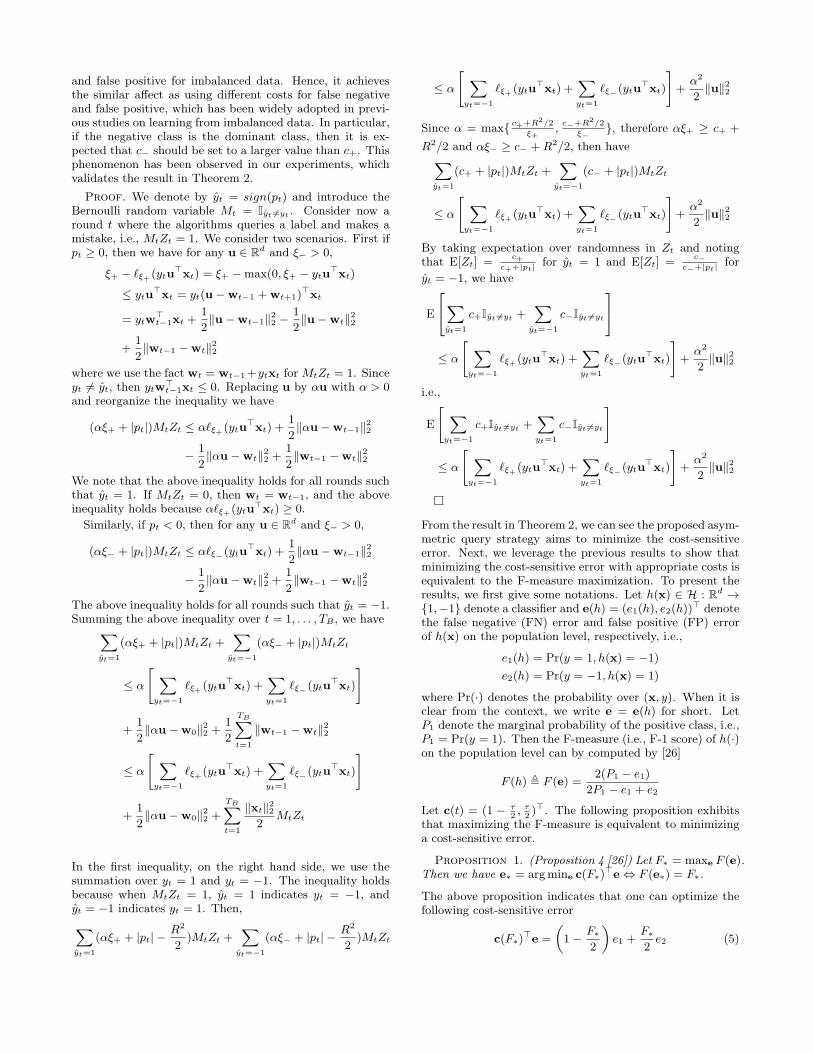
and false positive for imbalanced data. Hence, it achievesthe similar affect as using different costs for false negativeand false positive, which has been widely adopted in previ-ous studies on learning from imbalanced data. In particular,if the negative class is the dominant class, then it is ex-pected that c− should be set to a larger value than c+. Thisphenomenon has been observed in our experiments, whichvalidates the result in Theorem 2.

Proof. We denote by yt = sign(pt) and introduce theBernoulli random variable Mt = Iyt =yt . Consider now around t where the algorithms queries a label and makes amistake, i.e., MtZt = 1. We consider two scenarios. First ifpt ≥ 0, then we have for any u ∈ Rd and ξ− > 0,

ξ+ − ℓξ+(ytu⊤xt) = ξ+ −max(0, ξ+ − ytu

⊤xt)

≤ ytu⊤xt = yt(u−wt−1 +wt+1)

⊤xt

= ytw⊤t−1xt +

12∥u−wt−1∥22 −

12∥u−wt∥22

+12∥wt−1 −wt∥22

where we use the fact wt = wt−1+ytxt for MtZt = 1. Sinceyt = yt, then ytw

⊤t−1xt ≤ 0. Replacing u by αu with α > 0

and reorganize the inequality we have

(αξ+ + |pt|)MtZt ≤ αℓξ+(ytu⊤xt) +

12∥αu−wt−1∥22

− 12∥αu−wt∥22 +

12∥wt−1 −wt∥22

We note that the above inequality holds for all rounds suchthat yt = 1. If MtZt = 0, then wt = wt−1, and the aboveinequality holds because αℓξ+(ytu

⊤xt) ≥ 0.

Similarly, if pt < 0, then for any u ∈ Rd and ξ− > 0,

(αξ− + |pt|)MtZt ≤ αℓξ−(ytu⊤xt) +

12∥αu−wt−1∥22

− 12∥αu−wt∥22 +

12∥wt−1 −wt∥22

The above inequality holds for all rounds such that yt = −1.Summing the above inequality over t = 1, . . . , TB , we have

∑

yt=1

(αξ+ + |pt|)MtZt +∑

yt=−1

(αξ− + |pt|)MtZt

≤ α

[∑

yt=−1

ℓξ+(ytu⊤xt) +

∑

yt=1

ℓξ−(ytu⊤xt)

]

+12∥αu−w0∥22 +

12

TB∑

t=1

∥wt−1 −wt∥22

≤ α

[∑

yt=−1

ℓξ+(ytu⊤xt) +

∑

yt=1

ℓξ−(ytu⊤xt)

]

+12∥αu−w0∥22 +

TB∑

t=1

∥xt∥222

MtZt

In the first inequality, on the right hand side, we use thesummation over yt = 1 and yt = −1. The inequality holdsbecause when MtZt = 1, yt = 1 indicates yt = −1, andyt = −1 indicates yt = 1. Then,

∑

yt=1

(αξ+ + |pt|−R2

2)MtZt +

∑

yt=−1

(αξ− + |pt|−R2

2)MtZt

≤ α

[∑

yt=−1

ℓξ+(ytu⊤xt) +

∑

yt=1

ℓξ−(ytu⊤xt)

]+

α2

2∥u∥22

Since α = max{ c++R2/2

ξ+,c−+R2/2

ξ−}, therefore αξ+ ≥ c+ +

R2/2 and αξ− ≥ c− +R2/2, then have∑

yt=1

(c+ + |pt|)MtZt +∑

yt=−1

(c− + |pt|)MtZt

≤ α

[∑

yt=−1

ℓξ+(ytu⊤xt) +

∑

yt=1

ℓξ−(ytu⊤xt)

]+

α2

2∥u∥22

By taking expectation over randomness in Zt and notingthat E[Zt] =

c+c++|pt| for yt = 1 and E[Zt] =

c−c−+|pt| for

yt = −1, we have

E

⎡

⎣∑

yt=1

c+Iyt =yt +∑

yt=−1

c−Iyt =yt

⎤

⎦

≤ α

[∑

yt=−1

ℓξ+(ytu⊤xt) +

∑

yt=1

ℓξ−(ytu⊤xt)

]+

α2

2∥u∥22

i.e.,

E

[∑

yt=−1

c+Iyt =yt +∑

yt=1

c−Iyt =yt

]

≤ α

[∑

yt=−1

ℓξ+(ytu⊤xt) +

∑

yt=1

ℓξ−(ytu⊤xt)

]+

α2

2∥u∥22

From the result in Theorem 2, we can see the proposed asym-metric query strategy aims to minimize the cost-sensitiveerror. Next, we leverage the previous results to show thatminimizing the cost-sensitive error with appropriate costs isequivalent to the F-measure maximization. To present theresults, we first give some notations. Let h(x) ∈ H : Rd →{1,−1} denote a classifier and e(h) = (e1(h), e2(h))

⊤ denotethe false negative (FN) error and false positive (FP) errorof h(x) on the population level, respectively, i.e.,

e1(h) = Pr(y = 1, h(x) = −1)

e2(h) = Pr(y = −1, h(x) = 1)

where Pr(·) denotes the probability over (x, y). When it isclear from the context, we write e = e(h) for short. LetP1 denote the marginal probability of the positive class, i.e.,P1 = Pr(y = 1). Then the F-measure (i.e., F-1 score) of h(·)on the population level can by computed by [26]

F (h) ! F (e) =2(P1 − e1)

2P1 − e1 + e2

Let c(t) = (1 − τ2 ,

τ2 )

⊤. The following proposition exhibitsthat maximizing the F-measure is equivalent to minimizinga cost-sensitive error.

Proposition 1. (Proposition 4 [26]) Let F∗ = maxe F (e).Then we have e∗ = argmine c(F∗)

⊤e ⇔ F (e∗) = F∗.

The above proposition indicates that one can optimize thefollowing cost-sensitive error

c(F∗)⊤e =

(1− F∗

2

)e1 +

F∗

2e2 (5)

to obtain an optimal classifier h∗(x), which will give theoptimal F-measure, i.e., F (h∗) = F∗. However, the cost-sensitive error in (5) requires knowing the exact value ofthe optimal F-measure. To address this issue, we discretize(0, 1) to have a set of evenly distributed values {θ1, . . . , θK}such that θj+1 − θj = ϵ0/2. Then we can solve for a seriesof K classifiers to minimize the cost-senstive error

h∗j = argmin

h∈H

(1− θj

2

)e1 +

θj2e2 = c(θj)

⊤e, j = 1, . . . ,K

(6)

The following proposition shows that there exists one classi-fier among {h∗

j , · · · , h∗K} that can achieve a close-to-optimal

F-measure as long as ϵ0 is small enough.

Proposition 2. Let {θ1, . . . , θK} be a set of values evenlydistributed in (0, 1) such that θj+1 − θj = ϵ0/2. Then thereexists h∗

j ∈ {h∗j , · · · , h∗

K} such that

F (h∗j ) ≥ F∗ − 2ϵ0B

P1

where B = maxe ∥e∥2.

Remark: The above proposition is a corollary of Proposi-tion 5 in [26]. Note that the cost-sensitive error in (6) is justthe population level counterpart of the cost-sensitive error inTheorem 2, which further justifies the proposed asymmetricquery model.The above analysis implies that we can try different values

for the costs associated with the false negative error andfalse positive error, and use the cross-validation approach tochoose the best setting.

4. EXPERIMENT AND RESULTSIn order to investigate the algorithms on data of different

types, dimensionality, and proportion of positive examples,we conduct the experiment on 5 binary classification tasksfrom 3 datasets. All datasets are split as 2:1 for validationand testing respectively, with more information listed in Ta-ble 1. The validation data is used to tune the parametersin the compared algorithms. The testing data is used toevaluate the performance of different algorithms. On eachcollection, we evaluate the performance mainly through F1

score across the number of received examples. Also, we pro-vide both “query evaluation” and “query and push evalua-tion” according to the potential two types of label sources.

4.1 DataOne collection is cover type dataset from the UCI repos-

itory of Machine Learning databases. It contains 581,012examples and 7 classes of forest type, namely, Spruce-Fir,Lodgepole Pine, Ponderosa Pine, Cottonwood/Willow, As-pen, Douglas-fir, and Krummholz. Since the 7 classes havedistinct rates of positive examples, we conduct the exper-iment on three of them with different level of imbalanceto investigate the performance of algorithms. The threebinary classification problems are Ponderosa Pine vs NonPonderosa Pine, referred to as “cov1”, Spruce-Fir vs NonSpruce-Fir, referred to as “cov2”, and Lodgepole Pine vsNone Lodgepole Pine, referred to as “cov3”. From cov1,cov2 to cov3, the level of imbalance decreases. Detailed in-formation about the three tasks can be seen in Table 1.

Table 1: Statistics of five classification tasks# of examples Percentage # of

Validation Testing of Positive featurescov1 6.15cov2 387, 341 19, 3671 36.46 54cov3 48.76hd 155, 630 77815 6.25 313, 5392days 666, 667 333, 333 1.25 450, 065

Table 2: The best parameter values of different al-gorithms using PE

cov1 cov2 cov3 hd 2daysQA γ 0.1 0.1 0 10 0.1

c+ 0.005 0.01 0.1 1 0.01c− 0.01 0.1 0.1 10 1

QS γ 0.1 0 0 10 1c 0.01 0.1 0.1 10 0.1

QD γ 1 0 1 10 0c 0.01 0.01 0.01 100 0.01

QF γ 0 0 1 1 0.1QR γ 0 0.1 0.1 0 0CSOAL δ 0.01 0.01 0.1 0.1 0.1

We also evaluate our algorithm on two more datasetsfrom different domains, OHSUMED - a dataset of biomedi-cal publications, and 2 days’ tweets collected from Twitter.OHSUMED [17] is a well-known dataset, collecting 348, 543medical documents from MEDLINE from the year 1987 to1991. Each document consist of all or some of followingfields: MEDLINE identifier, MeSH terms, title, publicationtype, abstract, author, and source. Each document is asso-ciated with one or more MeSH terms, the medical subjectheading assigned by human. Since the MeSH term is orga-nized in a tree structure, we pick a subtree rooted at theMeSH term “Heart Disease” to be the positive class, andleave all the terms not in the subtree as negative. Specifi-cally, a document is a positive example if and only if it con-tains at least one MeSH term in the“Heart Disease” subtree.The task is referred to as hd.

The two days’ tweets, referred as 2days in the followingdiscussion, is a collection related to life satisfaction of theauthor of the tweets. It is collected by keywords such as “I”,“my”, etc. And each tweet is manually labeled as satisfy,dissatisfy, or irrelevant. We consider the binary classificationproblem of “related to the topic of life satisfaction” (positiveexample) or not relevant (negative example). Due to thenature of the data (e.g., tweet is a short text). this is adifficult task.

4.2 EvaluationAs we mentioned in the introduction section, we mainly

evaluate the algorithms by F1 score. Specifically, we plotthe accumulative F1 score along with the increase of theiteration. We also conduct two types of evaluation accord-ing to two types of label source. A push evaluation (PE)means that the labeling is independent from the use of theapplication, while push and query evaluation (PQE) meansthe labels are completely obtained from the user feedback.Specifically, in PE, only the examples such that yt = 1 arecounted as positive predication, and in PQE the queried ex-

(a) cov1, PE (b) cov2, PE (c) cov3, PE

(d) cov1, PQE (e) cov2, PQE (f) cov3, PQE

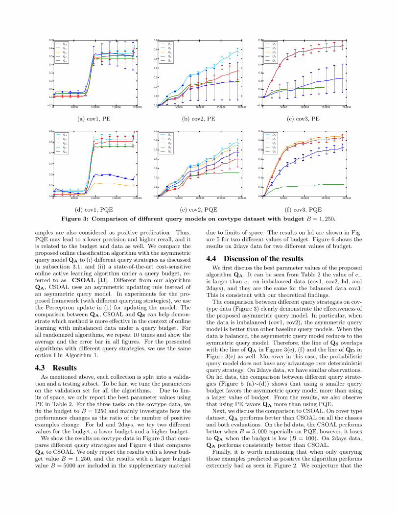
Figure 3: Comparison of different query models on covtype dataset with budget B = 1, 250.

amples are also considered as positive predication. Thus,PQE may lead to a lower precision and higher recall, and itis related to the budget and data as well. We compare theproposed online classification algorithm with the asymmetricquery model QA to (i) different query strategies as discussedin subsection 3.1; and (ii) a state-of-the-art cost-sensitiveonline active learning algorithm under a query budget, re-ferred to as CSOAL [33]. Different from our algorithmQA, CSOAL uses an asymmetric updating rule instead ofan asymmetric query model. In experiments for the pro-posed framework (with different querying strategies), we usethe Perceptron update in (1) for updating the model. Thecomparison between QA, CSOAL and QS can help demon-strate which method is more effective in the context of onlinelearning with imbalanced data under a query budget. Forall randomized algorithms, we repeat 10 times and show theaverage and the error bar in all figures. For the presentedalgorithms with different query strategies, we use the sameoption I in Algorithm 1.

4.3 ResultsAs mentioned above, each collection is split into a valida-

tion and a testing subset. To be fair, we tune the parameterson the validation set for all the algorithms. Due to lim-its of space, we only report the best parameter values usingPE in Table 2. For the three tasks on the covtype data, wefix the budget to B = 1250 and mainly investigate how theperformance changes as the ratio of the number of positiveexamples change. For hd and 2days, we try two differentvalues for the budget, a lower budget and a higher budget.We show the results on covtype data in Figure 3 that com-

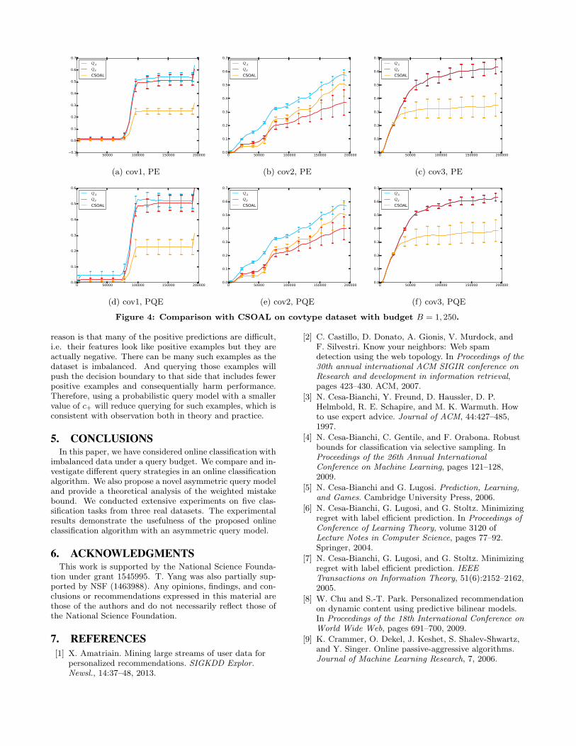
pares different query strategies and Figure 4 that comparesQA to CSOAL. We only report the results with a lower bud-get value B = 1, 250, and the results with a larger budgetvalue B = 5000 are included in the supplementary material

due to limits of space. The results on hd are shown in Fig-ure 5 for two different values of budget. Figure 6 shows theresults on 2days data for two different values of budget.

4.4 Discussion of the resultsWe first discuss the best parameter values of the proposed

algorithm QA. It can be seen from Table 2 the value of c−is larger than c+ on imbalanced data (cov1, cov2, hd, and2days), and they are the same for the balanced data cov3.This is consistent with our theoretical findings.

The comparison between different query strategies on cov-type data (Figure 3) clearly demonstrate the effectiveness ofthe proposed asymmetric query model. In particular, whenthe data is imbalanced (cov1, cov2), the asymmetric querymodel is better than other baseline query models. When thedata is balanced, the asymmetric query model reduces to thesymmetric query model. Therefore, the line of QS overlapswith the line of QA in Figure 3(e), (f) and the line of QD inFigure 3(e) as well. Moreover in this case, the probabilisticquery model does not have any advantage over deterministicquery strategy. On 2days data, we have similar observations.On hd data, the comparison between different query strate-gies (Figure 5 (a)∼(d)) shows that using a smaller querybudget favors the asymmetric query model more than usinga larger value of budget. From the results, we also observethat using PE favors QA more than using PQE.

Next, we discuss the comparison to CSOAL. On cover typedataset, QA performs better than CSOAL on all the classesand both evaluations. On the hd data, the CSOAL performsbetter when B = 5, 000 especially on PQE, however, it losesto QA when the budget is low (B = 100). On 2days data,QA performs consistently better than CSOAL.

Finally, it is worth mentioning that when only queryingthose examples predicted as positive the algorithm performsextremely bad as seen in Figure 2. We conjecture that the

(a) cov1, PE (b) cov2, PE (c) cov3, PE

(d) cov1, PQE (e) cov2, PQE (f) cov3, PQE

Figure 4: Comparison with CSOAL on covtype dataset with budget B = 1, 250.

reason is that many of the positive predictions are difficult,i.e. their features look like positive examples but they areactually negative. There can be many such examples as thedataset is imbalanced. And querying those examples willpush the decision boundary to that side that includes fewerpositive examples and consequentially harm performance.Therefore, using a probabilistic query model with a smallervalue of c+ will reduce querying for such examples, which isconsistent with observation both in theory and practice.

5. CONCLUSIONSIn this paper, we have considered online classification with

imbalanced data under a query budget. We compare and in-vestigate different query strategies in an online classificationalgorithm. We also propose a novel asymmetric query modeland provide a theoretical analysis of the weighted mistakebound. We conducted extensive experiments on five clas-sification tasks from three real datasets. The experimentalresults demonstrate the usefulness of the proposed onlineclassification algorithm with an asymmetric query model.

6. ACKNOWLEDGMENTSThis work is supported by the National Science Founda-

tion under grant 1545995. T. Yang was also partially sup-ported by NSF (1463988). Any opinions, findings, and con-clusions or recommendations expressed in this material arethose of the authors and do not necessarily reflect those ofthe National Science Foundation.

7. REFERENCES[1] X. Amatriain. Mining large streams of user data for

personalized recommendations. SIGKDD Explor.Newsl., 14:37–48, 2013.

[2] C. Castillo, D. Donato, A. Gionis, V. Murdock, andF. Silvestri. Know your neighbors: Web spamdetection using the web topology. In Proceedings of the30th annual international ACM SIGIR conference onResearch and development in information retrieval,pages 423–430. ACM, 2007.

[3] N. Cesa-Bianchi, Y. Freund, D. Haussler, D. P.Helmbold, R. E. Schapire, and M. K. Warmuth. Howto use expert advice. Journal of ACM, 44:427–485,1997.

[4] N. Cesa-Bianchi, C. Gentile, and F. Orabona. Robustbounds for classification via selective sampling. InProceedings of the 26th Annual InternationalConference on Machine Learning, pages 121–128,2009.

[5] N. Cesa-Bianchi and G. Lugosi. Prediction, Learning,and Games. Cambridge University Press, 2006.

[6] N. Cesa-Bianchi, G. Lugosi, and G. Stoltz. Minimizingregret with label efficient prediction. In Proceedings ofConference of Learning Theory, volume 3120 ofLecture Notes in Computer Science, pages 77–92.Springer, 2004.

[7] N. Cesa-Bianchi, G. Lugosi, and G. Stoltz. Minimizingregret with label efficient prediction. IEEETransactions on Information Theory, 51(6):2152–2162,2005.

[8] W. Chu and S.-T. Park. Personalized recommendationon dynamic content using predictive bilinear models.In Proceedings of the 18th International Conference onWorld Wide Web, pages 691–700, 2009.

[9] K. Crammer, O. Dekel, J. Keshet, S. Shalev-Shwartz,and Y. Singer. Online passive-aggressive algorithms.Journal of Machine Learning Research, 7, 2006.

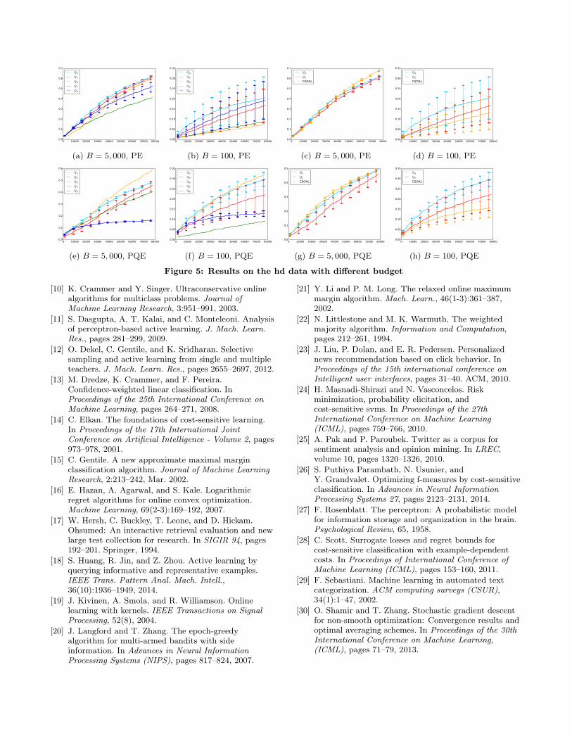
(a) B = 5, 000, PE (b) B = 100, PE (c) B = 5, 000, PE (d) B = 100, PE

(e) B = 5, 000, PQE (f) B = 100, PQE (g) B = 5, 000, PQE (h) B = 100, PQE

Figure 5: Results on the hd data with different budget

[10] K. Crammer and Y. Singer. Ultraconservative onlinealgorithms for multiclass problems. Journal ofMachine Learning Research, 3:951–991, 2003.

[11] S. Dasgupta, A. T. Kalai, and C. Monteleoni. Analysisof perceptron-based active learning. J. Mach. Learn.Res., pages 281–299, 2009.

[12] O. Dekel, C. Gentile, and K. Sridharan. Selectivesampling and active learning from single and multipleteachers. J. Mach. Learn. Res., pages 2655–2697, 2012.

[13] M. Dredze, K. Crammer, and F. Pereira.Confidence-weighted linear classification. InProceedings of the 25th International Conference onMachine Learning, pages 264–271, 2008.

[14] C. Elkan. The foundations of cost-sensitive learning.In Proceedings of the 17th International JointConference on Artificial Intelligence - Volume 2, pages973–978, 2001.

[15] C. Gentile. A new approximate maximal marginclassification algorithm. Journal of Machine LearningResearch, 2:213–242, Mar. 2002.

[16] E. Hazan, A. Agarwal, and S. Kale. Logarithmicregret algorithms for online convex optimization.Machine Learning, 69(2-3):169–192, 2007.

[17] W. Hersh, C. Buckley, T. Leone, and D. Hickam.Ohsumed: An interactive retrieval evaluation and newlarge test collection for research. In SIGIR 94, pages192–201. Springer, 1994.

[18] S. Huang, R. Jin, and Z. Zhou. Active learning byquerying informative and representative examples.IEEE Trans. Pattern Anal. Mach. Intell.,36(10):1936–1949, 2014.

[19] J. Kivinen, A. Smola, and R. Williamson. Onlinelearning with kernels. IEEE Transactions on SignalProcessing, 52(8), 2004.

[20] J. Langford and T. Zhang. The epoch-greedyalgorithm for multi-armed bandits with sideinformation. In Advances in Neural InformationProcessing Systems (NIPS), pages 817–824, 2007.

[21] Y. Li and P. M. Long. The relaxed online maximummargin algorithm. Mach. Learn., 46(1-3):361–387,2002.

[22] N. Littlestone and M. K. Warmuth. The weightedmajority algorithm. Information and Computation,pages 212–261, 1994.

[23] J. Liu, P. Dolan, and E. R. Pedersen. Personalizednews recommendation based on click behavior. InProceedings of the 15th international conference onIntelligent user interfaces, pages 31–40. ACM, 2010.

[24] H. Masnadi-Shirazi and N. Vasconcelos. Riskminimization, probability elicitation, andcost-sensitive svms. In Proceedings of the 27thInternational Conference on Machine Learning(ICML), pages 759–766, 2010.

[25] A. Pak and P. Paroubek. Twitter as a corpus forsentiment analysis and opinion mining. In LREC,volume 10, pages 1320–1326, 2010.

[26] S. Puthiya Parambath, N. Usunier, andY. Grandvalet. Optimizing f-measures by cost-sensitiveclassification. In Advances in Neural InformationProcessing Systems 27, pages 2123–2131, 2014.

[27] F. Rosenblatt. The perceptron: A probabilistic modelfor information storage and organization in the brain.Psychological Review, 65, 1958.

[28] C. Scott. Surrogate losses and regret bounds forcost-sensitive classification with example-dependentcosts. In Proceedings of International Conference ofMachine Learning (ICML), pages 153–160, 2011.

[29] F. Sebastiani. Machine learning in automated textcategorization. ACM computing surveys (CSUR),34(1):1–47, 2002.

[30] O. Shamir and T. Zhang. Stochastic gradient descentfor non-smooth optimization: Convergence results andoptimal averaging schemes. In Proceedings of the 30thInternational Conference on Machine Learning,(ICML), pages 71–79, 2013.

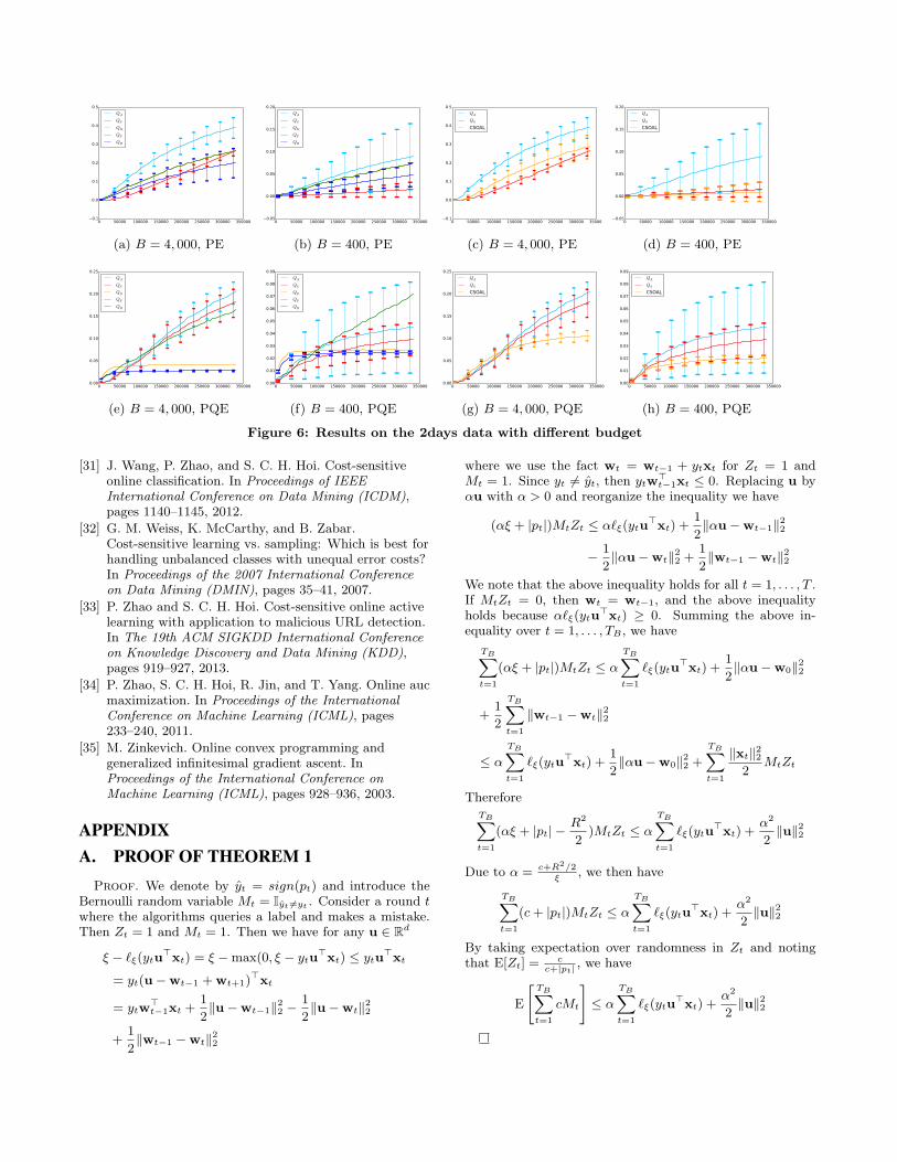
(a) B = 4, 000, PE (b) B = 400, PE (c) B = 4, 000, PE (d) B = 400, PE

(e) B = 4, 000, PQE (f) B = 400, PQE (g) B = 4, 000, PQE (h) B = 400, PQE

Figure 6: Results on the 2days data with different budget

[31] J. Wang, P. Zhao, and S. C. H. Hoi. Cost-sensitiveonline classification. In Proceedings of IEEEInternational Conference on Data Mining (ICDM),pages 1140–1145, 2012.

[32] G. M. Weiss, K. McCarthy, and B. Zabar.Cost-sensitive learning vs. sampling: Which is best forhandling unbalanced classes with unequal error costs?In Proceedings of the 2007 International Conferenceon Data Mining (DMIN), pages 35–41, 2007.

[33] P. Zhao and S. C. H. Hoi. Cost-sensitive online activelearning with application to malicious URL detection.In The 19th ACM SIGKDD International Conferenceon Knowledge Discovery and Data Mining (KDD),pages 919–927, 2013.

[34] P. Zhao, S. C. H. Hoi, R. Jin, and T. Yang. Online aucmaximization. In Proceedings of the InternationalConference on Machine Learning (ICML), pages233–240, 2011.

[35] M. Zinkevich. Online convex programming andgeneralized infinitesimal gradient ascent. InProceedings of the International Conference onMachine Learning (ICML), pages 928–936, 2003.

APPENDIXA. PROOF OF THEOREM 1

Proof. We denote by yt = sign(pt) and introduce theBernoulli random variable Mt = Iyt =yt . Consider a round twhere the algorithms queries a label and makes a mistake.Then Zt = 1 and Mt = 1. Then we have for any u ∈ Rd

ξ − ℓξ(ytu⊤xt) = ξ −max(0, ξ − ytu

⊤xt) ≤ ytu⊤xt

= yt(u−wt−1 +wt+1)⊤xt

= ytw⊤t−1xt +

12∥u−wt−1∥22 −

12∥u−wt∥22

+12∥wt−1 −wt∥22

where we use the fact wt = wt−1 + ytxt for Zt = 1 andMt = 1. Since yt = yt, then ytw

⊤t−1xt ≤ 0. Replacing u by

αu with α > 0 and reorganize the inequality we have

(αξ + |pt|)MtZt ≤ αℓξ(ytu⊤xt) +

12∥αu−wt−1∥22

− 12∥αu−wt∥22 +

12∥wt−1 −wt∥22

We note that the above inequality holds for all t = 1, . . . , T .If MtZt = 0, then wt = wt−1, and the above inequalityholds because αℓξ(ytu

⊤xt) ≥ 0. Summing the above in-equality over t = 1, . . . , TB , we have

TB∑

t=1

(αξ + |pt|)MtZt ≤ αTB∑

t=1

ℓξ(ytu⊤xt) +

12∥αu−w0∥22

+12

TB∑

t=1

∥wt−1 −wt∥22

≤ αTB∑

t=1

ℓξ(ytu⊤xt) +

12∥αu−w0∥22 +

TB∑

t=1

∥xt∥222

MtZt

ThereforeTB∑

t=1

(αξ + |pt|−R2

2)MtZt ≤ α

TB∑

t=1

ℓξ(ytu⊤xt) +

α2

2∥u∥22

Due to α = c+R2/2ξ , we then have

TB∑

t=1

(c+ |pt|)MtZt ≤ αTB∑

t=1

ℓξ(ytu⊤xt) +

α2

2∥u∥22

By taking expectation over randomness in Zt and notingthat E[Zt] = c

c+|pt| , we have

E

[TB∑

t=1

cMt

]≤ α

TB∑

t=1

ℓξ(ytu⊤xt) +

α2

2∥u∥22