Online and Offline Algorithms for the Time-Dependent TSP with Time Zones

DOI: 10.1007/s00453-004-1088-z

Algorithmica (2004) 39: 299–319 Algorithmica© 2004 Springer-Verlag New York, LLC

Online and Offline Algorithms for the Time-DependentTSP with Time Zones

Bjorn Broden,1 Mikael Hammar,2 and Bengt J. Nilsson3

Abstract. The time-dependent traveling salesman problem (TDTSP) is a variant of TSP with time-dependentedge costs. We study some restrictions of TDTSP where the number of edge cost changes are limited. Wefind competitive ratios for online versions of TDTSP. From these we derive polynomial time approximationalgorithms for graphs with edge costs one and two. In addition, we present an approximation algorithm for theorienteering problem with edge costs one and two.

Key Words. Online algorithms, The traveling salesman problem, Time dependencies, The orienteeringproblem.

1. Introduction. Transportation and scheduling problems modeled by the travelingsalesman problem (TSP) are inherently static. To model a dynamic environment a gener-alization is needed that incorporates changes in the environment. Such a generalizationis provided by the time-dependent traveling salesman problem (TDTSP). This problemis a generalization of TSP in which the cost of each edge depends on time, i.e., the cost ofan edge depends on the time interval during which the edge is traversed. Several aspectsof TDTSP have been studied and it seems to be difficult to collect them all under a singledefinition. The many variations all stem from the way that time is modeled.

In some definitions time is proportional to the cost of the edges traversed [12]. Thisgives a natural generalization of TSP and is suitable if for example variations in thetraffic load are important in computing a TSP tour for a delivery company. It also hasconnections to other generalizations of TSP, such as the kinetic TSP where movingpoints in the plane [9], [10] or on a line [10] are considered. We call this formulation thecost-dependent traveling salesman problem (CDTSP).

Our focus is on another formulation of TDTSP where the cost of an edge dependson its position in the path. We call this problem the step-dependent traveling salesmanproblem, denoted SDTSP. This interpretation has been studied on numerous occasionsby the operations research community, due to its application in scheduling [3], [5], [6],[14]. We limit our study of TDTSP to instances where the edge costs are restricted insize and can change only a limited number of times.

1 Department of Computer Science, Lund University, Box 118, S-221 00 Lund, Sweden. [email protected] Dipartimento di Informatica ed Applicazioni, Universita di Salerno, Baronissi (SA) 84081, [email protected] School of Technology and Society, Malmo University College, SE-205 06 Malmo, Sweden. [email protected].

Received October 7, 2002; revised November 27, 2003. Communicated by S. Albers.Online publication March 29, 2004.

300 B. Broden, M. Hammar, and B. J. Nilsson

Due to complications caused by time dependencies, approximation algorithms forTDTSP are hard to analyze. By considering online algorithms part of the time dependencyis removed and a more tractable structure is achieved. Online algorithms for TSP havebeen studied in the past [2], [4], [11]. These algorithms take a set of cities as input, andcompute the shortest TSP tour. Over time, new cities are added to the set. We studyTSP in a dynamic environment; although the cities are known from the beginning, thedistance between a pair of cities changes over time.

The online algorithms we present here still require a solution to the NP-hard orienteer-ing problem [1]. As we shall see in Section 5 this problem allows a 3/4-approximationalgorithm for graphs with edge costs one and two. We construct a polynomial time ap-proximation algorithm for SDTSP by choosing the best answer given by a set of onlinealgorithms. This results in a (2− 2/3k)-approximation algorithm for the SDTSP wherethe edge costs are restricted to the values one and two and the costs can change at mostk−1 times. The restrictions on the edge costs can be removed given an orienteering algo-rithm that handles arbitrary edge costs. Since the inapproximability ratio of TSP growswith the relative edge costs we cannot expect algorithms for SDTSP with approximationratio independent of the costs.

In Section 2 we state the formal definition of SDTSP. In Section 3 we analyze the on-line version of the problem and in Section 4 we consider polynomial time approximationalgorithms. We also give an approximation algorithm for the orienteering problem foredge costs one and two. In Section 5 we consider CDTSP. We give an inapproximabilityresult for the Euclidean CDTSP and present an online algorithm for CDTSP with twotime zones and edge costs one and two. This online algorithm is modified to give anapproximation algorithm as in the previous section.

2. Definition of SDTSP

DEFINITION 1. Consider a set of edge cost functions {c1, . . . , cn} assigned to a completegraph G = (V, E)with |V | = n, |E | = (n

2

), and where ct (e) is the cost function for edge

e ∈ E . Let ei j denote the edge between vi and vj in V . The step-dependent travelingsalesman problem (SDTSP) seeks a permutation π of V that minimizes

cn(eπnπ1)+n−1∑

i=1

ci (eπiπi+1).

In order to comprehend Definition 1 it helps to consider an instance of SDTSP asan n-layered graph, each layer containing n vertices. Layer i and layer i + 1 form acomplete bipartite graph where the edges are directed, going from layer i to layer i + 1,and are given weights according to weight function ci . The objective is to find a pathgoing from layer one to layer n that visits all columns, starting from and ending at thesame column.

We can view ct as a discrete time-dependent edge cost function defined on t ={1, . . . , n}. To simplify the problem we restrict our study to the case where this cost

Online and Offline Algorithms for the Time-Dependent TSP with Time Zones 301

function changes at most k−1 times as a function of t . A region where the cost functionis constant is called a time zone. Let 0 = z0, z1, . . . , zk−1, zk = n ∈ N denote the timezone divisors, i.e., time zone i = {zi−1+1, . . . , zi }, and cj = cj ′ for zi−1 < j, j ′ ≤ zi .We simplify the representation by assigning one cost function to each time zone, givingus an instance I = {(c1, z1), . . . , (ck, zk)}. An instance of SDTSP with k time zones isdenoted SDkTSP. Let M and m denote the costs of the most and least expensive edgesusing any of the cost functions c1, . . . , ck .

We primarily study the online version of SDkTSP for which an algorithm receivesinformation regarding the time zones and the cost functions online. Let Ij = (cj , zj )

represent the instance restricted to time zone j , i.e., I = {I1, . . . , Ik}. The algorithmreceives the input instance one time zone at a time. For each time zone j it producesa path Pj that contains zj − zj−1 previously unvisited vertices and with edge weightsgiven by cj . When Pj has been computed, the algorithm receives the next part of theinput instance, i.e., Ij+1. After k time zones the algorithm has received the entire inputinstance and a Hamilton cycle in G has been built.

DEFINITION 2. Given an arbitrary algorithm A for SDkTSP we write A[I ] for the ver-tices of the cycle that the algorithm chooses on the instance I and A(I ) for the cost ofthe resulting cycle produced on I . This will also be used for specific time zones, forinstance A(I1) is the cost of the path in time zone one.

Let A j [I ] = ∪ ji=1 A[Ii ], i.e., the vertices that A chooses from time zone one to time

zone j .

DEFINITION 3. Let R(A) denote the competitive ratio for algorithm A and let R be thesmallest competitive ratio for any online algorithm, i.e., R = minA{R(A)}. We use ALGto denote an arbitrary online algorithm, OFF to denote an arbitrary offline algorithm,and OPT to denote the optimal offline algorithm for SDkTSP.

3. Online SDkTSP. Here we present a lower bound on the competitive ratio forSDkTSP. We also present a strategy with a competitive ratio matching the lower bound.To compute the lower bound we use an adversary argument. The adversary builds a hardinstance for the strategy. This is done online in response to the decisions made by thestrategy. Let I z denote the instance created by the adversary. In addition to this instancewe define an adversary offline algorithm ZIG. This algorithm is adapted both to I z and tothe decisions that were made by the online strategy being analyzed. We can think of theadversary algorithm as being run in hindsight after the completion of the online strategy.Note that ZIG is designed to be optimal for I z .

The adversary constructs the instance I z as follows: all edge costs in I z1 are set to m.

In I zj , for 2 ≤ j ≤ k, all costs of edges adjacent to vertices in ALG j−1[I z] are set to m

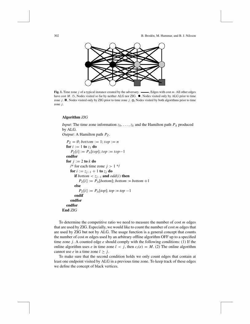
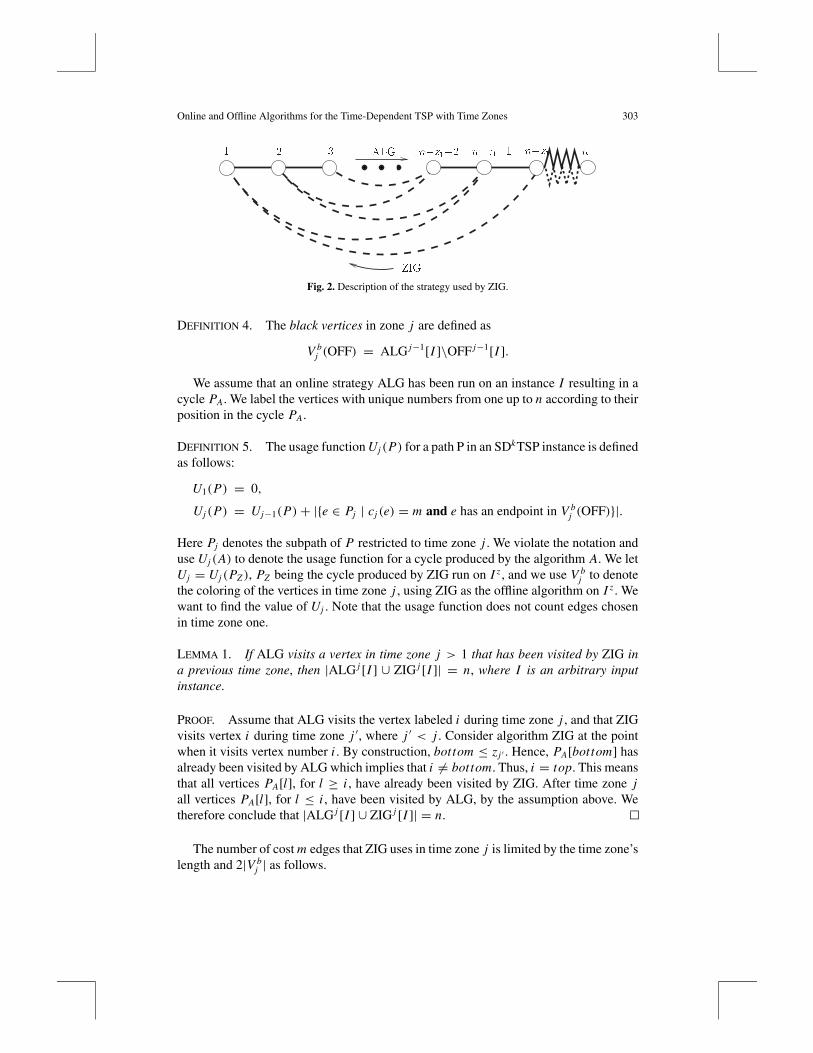
and all other edge costs are set to M . Time zone j of a typical instance I z is shown inFigure 1. The algorithm ZIG is designed to maximize the number of cost m edges used.It is described below and its strategy for time zone j is illustrated in Figure 2.


Fig. 1. Time zone j of a typical instance created by the adversary. , Edges with cost m. All other edgeshave cost M . , Nodes visited so far by neither ALG nor ZIG. , Nodes visited only by ALG prior to timezone j . , Nodes visited only by ZIG prior to time zone j . , Nodes visited by both algorithms prior to timezone j .

Algorithm ZIG

Input: The time zone information z0, . . . , zk and the Hamilton path PA producedby ALG.Output: A Hamilton path PZ .

PZ = ∅; bottom := 1; top := nfor i := 1 to z1 do

PZ [i] := PA[top]; top := top−1endforfor j := 2 to k do

/* for each time zone j > 1 */for i := zj−1 + 1 to zj do

if bottom < zj−1 and odd(i) thenPZ [i] := PA[bottom]; bottom := bottom +1

elsePZ [i] := PA[top]; top := top −1

endifendfor

endforEnd ZIG

To determine the competitive ratio we need to measure the number of cost m edgesthat are used by ZIG. Especially, we would like to count the number of cost m edges thatare used by ZIG but not by ALG. The usage function is a general concept that countsthe number of cost m edges used by an arbitrary offline algorithm OFF up to a specifiedtime zone j . A counted edge e should comply with the following conditions: (1) If theonline algorithm uses e in time zone l < j , then cl(e) = M . (2) The online algorithmcannot use e in a time zone l ≥ j .

To make sure that the second condition holds we only count edges that contain atleast one endpoint visited by ALG in a previous time zone. To keep track of these edgeswe define the concept of black vertices.


321

ZIG

ALG nn�z1�2 n�z1�1 n�z1

Fig. 2. Description of the strategy used by ZIG.

DEFINITION 4. The black vertices in zone j are defined as

V bj (OFF) = ALG j−1[I ]\OFF j−1[I ].

We assume that an online strategy ALG has been run on an instance I resulting in acycle PA. We label the vertices with unique numbers from one up to n according to theirposition in the cycle PA.

DEFINITION 5. The usage function Uj (P) for a path P in an SDkTSP instance is definedas follows:

U1(P) = 0,

Uj (P) = Uj−1(P)+ |{e ∈ Pj | cj (e) = m and e has an endpoint in V bj (OFF)}|.

Here Pj denotes the subpath of P restricted to time zone j . We violate the notation anduse Uj (A) to denote the usage function for a cycle produced by the algorithm A. We letUj = Uj (PZ ), PZ being the cycle produced by ZIG run on I z , and we use V b

j to denotethe coloring of the vertices in time zone j , using ZIG as the offline algorithm on I z . Wewant to find the value of Uj . Note that the usage function does not count edges chosenin time zone one.

LEMMA 1. If ALG visits a vertex in time zone j > 1 that has been visited by ZIG ina previous time zone, then |ALG j [I ] ∪ ZIG j [I ]| = n, where I is an arbitrary inputinstance.

PROOF. Assume that ALG visits the vertex labeled i during time zone j , and that ZIGvisits vertex i during time zone j ′, where j ′ < j . Consider algorithm ZIG at the pointwhen it visits vertex number i . By construction, bottom ≤ zj ′ . Hence, PA[bottom] hasalready been visited by ALG which implies that i �= bottom. Thus, i = top. This meansthat all vertices PA[l], for l ≥ i , have already been visited by ZIG. After time zone jall vertices PA[l], for l ≤ i , have been visited by ALG, by the assumption above. Wetherefore conclude that |ALG j [I ] ∪ ZIG j [I ]| = n.

The number of cost m edges that ZIG uses in time zone j is limited by the time zone’slength and 2|V b

j | as follows.


LEMMA 2. The number of cost m edges counted by Uj (OFF) in time zone j > 1 is atmost

min{2|V bj (OFF)|, zj − zj−1}.

PROOF. Let P be the cycle generated by OFF and let Pj be the subpath of P in timezone j . All edges counted by Uj (OFF) in time zone j belong to Pj by definition, and|Pj | = zj − zj−1. Secondly, all edges counted by Uj (OFF) in time zone j have atleast one endpoint in V b

j (OFF). This implies that each vertex in V bj (OFF) is adjacent

to at most two counted edges. It follows that the number of cost m edges counted is atmost 2|V b

j (OFF)|.

LEMMA 3. The number of cost m edges counted by Uj in time zone j > 1 is exactly

min{2|V bj |, zj − zj−1}.

PROOF. From Lemma 2 it follows that ZIG uses at most min{2|V bj |, zj − zj−1} cost m

edges in time zone j . To see that ZIG uses at least min{2|V bj |, zj − zj−1} cost m edges

of I z we need to examine the algorithm in detail.If |ALG j−1[I z] ∪ ZIG j [I z]| = n, then all edges taken by ZIG in time zone j have

endpoints in ALG j−1[I z] and by definition, these edges have cost m in I z . Hence, exactlyzj − zj−1 cost m edges are counted by Uj in time zone j .

If |ALG j−1[I z] ∪ ZIG j [I z]| < n, then there are vertices neither visited by ALG in atime zone prior to j nor by ZIG in a time zone prior to j + 1. Let tj denote the value oftop and bj the value of bottom at the beginning of time zone j and let t ′j and b′j denote thecorresponding values at the end of the time zone. Now, zj−1 is the index of the last vertexvisted by ALG in time zone j − 1, and, since there are unvisited vertices left, t ′j > zj−1.The black vertices therefore have the labels bj , . . . , zj−1. Thus, zj−1 − bj + 1 = |V b

j |.Furthermore, any vertex taken from the top of PA has not been visited yet by ALG.

Consider algorithm ZIG at the beginning of time zone j . Every time bottom isincreased, a black vertex is incorporated into ZIG’s path. Every time top is decreased,a vertex unvisited by ALG is inserted into the path. Thus, every second vertex pickedis black save perhaps a string of uncolored vertices at the end. If exactly every secondvertex in the path constructed for time zone j is black, then all zj − zj−1 edges arecounted by Uj . If less than every second vertex is black, then the if-statement inside thefor-loop has been violated more than (zj − zj−1)/2 times and we infer that b′j = zj−1.Thus, bottom has been increased |V b

j | times and all black vertices lie on the subpath ofPZ in time zone j . For every black vertex, two edges are counted by Uj . In this case2|V b

j | edges are counted.

Lemma 2 gives the following upper bound on Uj (OFF).

LEMMA 4. Uj (OFF) is given by the following recurrence relation:

U1(OFF) ≤ 0

Uj (OFF) ≤ Uj−1(OFF)+min{2|V bj (OFF)|, zj − zj−1} if 2 ≤ j ≤ k.


Lemma 3 gives us a recurrence relation for Uj similar to the upper bound on Uj (OFF).

LEMMA 5. Uj is given by the following recurrence relation:

U1 = 0

Uj = Uj−1 +min{2|V bj |, zj − zj−1} if 2 ≤ j ≤ k.

To evaluate the recurrence we would like to express |V bj | in terms of Uj−1 and zj−1.

To this end we use the following lemma.

LEMMA 6. If 2|V bj | < zj − zj−1, then |ALG j−1[I z] ∪ ZIG j−1[I z]| < n.

PROOF. At the beginning of time zone j , the number of vertices visited by ALG but notby ZIG is |V b

j |. The number of vertices visited by ZIG in previous time zones is zj−1.Therefore,

|ALG j−1[I z] ∪ ZIG j−1[I z]| = |ALG j−1[I z]\ZIG j−1[I z]| + |ZIG j−1[I z]|= |V b

j | + zj−1

≤ 2|V bj | + zj−1

< zj − zj−1 + zj−1 = zj ≤ n.

LEMMA 7. If 2|V bj | < zj − zj−1, then Uj−1 = 2|ALG j−1[I z] ∩ ZIG j−1[I z]|.

PROOF. If 2|V bj | < zj − zj−1, then |ALG j−1[I z] ∪ ZIG j−1[I z]| < n, according to

Lemma 6. From Lemma 1 it follows that prior to time zone j , ALG has never visited avertex already visited by ZIG. We infer two consequences from this fact, the first beingthat all vertices in ALG j−1[I z] ∩ ZIG j−1[I z] were black when ZIG visited them. Thesecond consequence is that top > zj−1 at the end of time zone j − 1. This implies thatno edge in the path produced by ZIG has two endpoints in ALG j−1[I z] ∩ ZIG j−1[I z].The number of edges incident to vertices in ALG j−1[I z] ∩ ZIG j−1[I z] is therefore2|ALG j−1[I z] ∩ ZIG j−1[I z]| and all of them are counted by Uj−1, since Uj−1 onlycounts edges that ALG has already visited. Hence, the result follows.

Now we can find a simpler expression for U using the following transformation.If 2|V b

j | < zj − zj−1, then |V bj | = |ALG j−1[I z]| − |ALG j−1[I z] ∩ ZIG j−1[I z]| =

zj−1 −Uj−1/2, by Lemma 7. We have proved the following theorem.

THEOREM 1. The usage function of ZIG is equal to

U1 = 0,

Uj = Uj−1 +min{2zj−1 −Uj−1, zj − zj−1} if 2 ≤ j ≤ k.

Given Theorem 1 we compute a maximum value of Uk .


THEOREM 2. The maximum value of the function Uk is Uk = n − z1 and occurswhen zi = (2i − 1)n/(2k − 1).

PROOF. Assuming U0 = 0 we have that

Uj = Uj−1 +min{2zj−1 −Uj−1, zj − zj−1}.

Uj is maximized if 2zj−1 −Uj−1 = zj − zj−1. That is,

Uj = 2zj−1,(3.0.1)

Uj = Uj−1 + zj − zj−1.(3.0.2)

Substituting Uj with 2zj−1 in (3.0.2) yields

zj − 3zj−1 + 2zj−2 = 0.

We solve the equation given that z0 = 0 and zk = n:

zj = 2 j − 1

2k − 1n.

After substituting zj accordingly in (3.0.1) we have that

Uk = n − z1,

since z1 = n/(2k − 1).

We state a final lemma concerning the usage function for any offline algorithm OFF.We use this to prove upper bounds on online algorithms for SDkTSP.

LEMMA 8. Let 0=z0, z1, . . . , zj≤n ∈ N. For any instance I = {(c1, z1), . . . , (cj , zj )}of SDkTSP and any offline algorithm OFF,

Uj (OFF) ≤ Uj .

PROOF. By definition U1(OFF) = U1 = 0.For j > 1, assume that Uj−1(OFF) ≤ Uj−1. By definition, Uj−1 counts the number

of low cost edges visited by OFF in time zone j ′ < j having at least one endpoint inALG j ′−1[I ]. The number of such vertices is at least Uj−1/2, and hence,

Uj−1

2≤ |ALG j ′−1[I ] ∩ OFF j ′ [I ]|

≤ |ALG j−1[I ] ∩ OFF j−1[I ]|= |ALG j−1[I ]| − |ALG j−1[I ]\OFF j−1[I ]|= zj−1 − |V b

j (OFF)|.


From Lemma 4 and our induction hypothesis we have that

Uj (OFF) ≤ Uj−1(OFF)+min{2|V bj (OFF)|, zj − zj−1}

≤ Uj−1(OFF)+min{2zj−1 −Uj−1(OFF), zj − zj−1}= min{2zj−1, zj − zj−1 +Uj−1(OFF)}≤ min{2zj−1, zj − zj−1 +Uj−1}= Uj−1 +min{2zj−1 −Uj−1, zj − zj−1}= Uj .

3.1. Lower Bound on the Competitive Ratio. This section uses the results we havearrived at so far to state the first of our main results.

THEOREM 3. The competitive ratio, R, of any online algorithm for SDkTSP is

R ≥ 1+ (M − m)Uk

ZIG(I z).

PROOF. Consider an arbitrary online strategy ALG. To analyze the competitive ratiowe use our adversary argument, including the instance I z together with the adversaryalgorithm ZIG. The online algorithm has to pay M on all edges except those usedin time zone one, since edges with cost set to m in other zones can only be used byZIG. The cost for ZIG on the instance I z is ZIG(I z) = mUk + M(n − (Uk + z1))

= Mn − (M − m)(Uk + z1), giving us the competitive ratio

R = minALG

maxI

ALG(I )

OPT(I )≥ min

ALG

ALG(I z)

ZIG(I z)≥ M(n − z1)+ mz1

ZIG(I z).

Doing the calculations backwards we get that

R ≥ M(n − z1)+ mz1 − Mn + (M − m)(Uk + z1)+ ZIG(I z)

ZIG(I z)

= 1+ (M − m)Uk

ZIG(I z).

Applying Theorem 2 to Theorem 3 produces the following corollary.

COROLLARY 1. The worst-case competitive ratio R of any strategy ALG on any instanceI = {(c1, z1), . . . , (ck, zk)} is at least

R ≥ M

m· 2k − 2

2k − 1+ 1

2k − 1.

3.2. Upper Bound on the Competitive Ratio. There is a simple strategy that achievesthe upper bound found in the last section. This algorithm, presented below, uses a greedyapproach.


Algorithm GREEDY for SDkTSP.

Input: A sequence of k instances I1, . . . , Ik .Output: A Hamilton cycle P .

1 Given an instance Ij , produce the cheapest path of size zj − zj−1 on theunvisited vertices in V .

End GREEDY for SDkTSP.

THEOREM 4. The competitive ratio of GREEDY as a function of Uk is at most

1+maxI

(M − m)Uk

OPT(I ).

PROOF. Let I be an arbitrary SDkTSP instance, and let PI be the optimal TSP touron I . In time zone one GREEDY(I1) = OPT(I1). Assume that the following holds forj > 1:

GREEDY(Ij ) ≤ OPT(Ij )+ (M − m)(Uj (PI )−Uj−1(PI )).

Summing up the inequalities (including time zone one) yields that

k∑

i=1

GREEDY(Ii ) ≤ OPT(I )+ (M − m)(Uk(PI ))

≤ OPT(I )+ (M − m)Uk,

according to Lemma 8. This gives a competitive ratio of

R(GREEDY) ≤ maxI

OPT(I )+ (M − m)Uk

OPT(I )= 1+max

I

(M − m)Uk

OPT(I ).

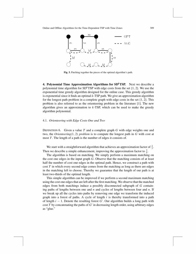
It remains to prove our assumed inequality. This is equivalent to showing that there isa path usable by GREEDY in time zone j > 1 that costs at most OPT(Ij ) + ((M −m)(U (OPT j [I ])−U (OPT j−1[I ])). First observe that the number of edges counted bythe usage function in time zone j is Uj (PI )−Uj−1(PI ). OPT pays at least m(Uj (PI )−Uj−1(PI )) for these edges. This cost is included in OPT j [I ]. Edges not counted by theusage function can be used by ALG for the same cost as OPT. These edges are connectedwith possibly expensive edges for a total cost of OPT(Ij )+(M−m)(Uj (PI )−Uj−1(PI ));see Figure 3. By construction GREEDY finds a path having at most this cost.

This theorem together with Theorem 3 gives a sharp worst-case competitive ratio.

COROLLARY 2. The competitive ratio of GREEDY is

R = M

m· 2k − 2

2k − 1+ 1

2k − 1.

Note that we have no implementation of GREEDY that runs in polynomial time, sinceit contains an NP-complete subproblem.


m

m

ALG

OPT

M

MM

m

M

m

m

mm

Fig. 3. Patching together the pieces of the optimal algorithm’s path.

4. Polynomial Time Approximation Algorithms for SDkTSP. Next we describe apolynomial time algorithm for SDkTSP with edge costs from the set {1, 2}. We use theexponential time greedy algorithm designed for the online case. This greedy algorithmis exponential since it finds an optimal k-TSP path. We give an approximation algorithmfor the longest path problem in a complete graph with edge costs in the set {1, 2}. Thisproblem is also referred to as the orienteering problem in the literature [1]. The newalgorithm gives an approximation to k-TSP, which can be used to make the greedyalgorithm polynomial.

4.1. Orienteering with Edge Costs One and Two

DEFINITION 6. Given a value T and a complete graph G with edge weights one andtwo, the Orienteering(1, 2) problem is to compute the longest path in G with cost atmost T . The length of a path is the number of edges it consists of.

We start with a straightforward algorithm that achieves an approximation factor of 23 .

Then we describe a simple enhancement, improving the approximation factor to 34 .

The algorithm is based on matching. We simply perform a maximum matching onthe cost one edges in the input graph G. Observe that the matching consists of at leasthalf the number of cost one edges in the optimal path. Hence, we construct a path withcost T in which every second edge comes from the matching as long as there are edgesin the matching left to choose. Thereby we guarantee that the length of our path is atleast two-thirds of the optimal length.

This simple algorithm can be improved if we perform a second maximum matchingusing the cost one edges that are left after the first matching. We observe that the matchededges from both matchings induce a possibly disconnected subgraph of G contain-ing paths of lengths between one and n and cycles of lengths between four and n. Ifwe break up all the cycles into paths by removing one edge we transform the inducedgraph into a forest of paths. A cycle of length i is thereby transformed into a pathof length i − 1. Denote the resulting forest G ′. Our algorithm builds a long path withcost T by concatenating the paths of G ′ in decreasing length order, using arbitrary edgesas “glue.”


Algorithm Enhanced Orienteering(1, 2)

Input: A value T and a complete graph G = (V, E) with edge costs eitherone or two.Output: A path with cost T .

1 E1 ← A maximum matching on the cost one edges in G.2 E2 ← A maximum matching on the remaining cost one edges in G.3 G ′ ← (V, E1 ∪ E2)

4 Break up the cycles in G ′ as described above.5 Construct a Hamilton path H of G by concatenating the paths in G ′ in

decreasing length order, appending the remaining cost two edges to theend.

6 return the longest (initial) part of H with cost less or equal to T .

End Enhanced Orienteering(1, 2)

The time complexity of this algorithm is dominated by the maximum matching pro-cedure, which is polynomial [7].

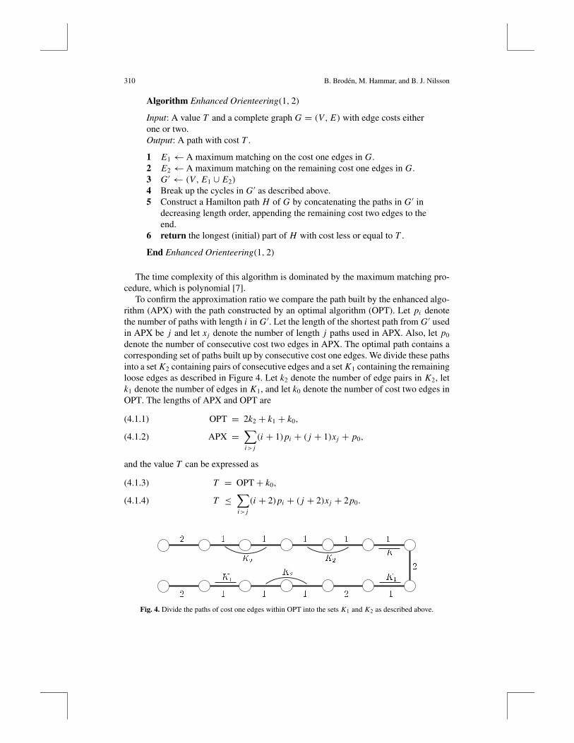
To confirm the approximation ratio we compare the path built by the enhanced algo-rithm (APX) with the path constructed by an optimal algorithm (OPT). Let pi denotethe number of paths with length i in G ′. Let the length of the shortest path from G ′ usedin APX be j and let xj denote the number of length j paths used in APX. Also, let p0

denote the number of consecutive cost two edges in APX. The optimal path contains acorresponding set of paths built up by consecutive cost one edges. We divide these pathsinto a set K2 containing pairs of consecutive edges and a set K1 containing the remainingloose edges as described in Figure 4. Let k2 denote the number of edge pairs in K2, letk1 denote the number of edges in K1, and let k0 denote the number of cost two edges inOPT. The lengths of APX and OPT are

OPT = 2k2 + k1 + k0,(4.1.1)

APX =∑

i> j

(i + 1)pi + ( j + 1)xj + p0,(4.1.2)

and the value T can be expressed as

T = OPT+ k0,(4.1.3)

T ≤∑

i> j

(i + 2)pi + ( j + 2)xj + 2p0.(4.1.4)

K2

K1 K1

K1

K2

K2

1

2

2

21 11

2 1 1 1 1

1

Fig. 4. Divide the paths of cost one edges within OPT into the sets K1 and K2 as described above.


Let A denote the number of cost one edges in G ′ that originate from the first maximummatching. Let B denote the number of cost one edges from the second matching in G ′.The following lemma describes crucial relations regarding the number of edges matchedby the algorithm, the number of paths in G ′ and the number of cost one edges in OPT.

LEMMA 9. The following four conditions hold:

B ≤∑

i>1

(i − 1)pi ,(4.1.5)

A >3k1 + 6k2

8,(4.1.6)

B ≥ k2,(4.1.7)

A + B =∑

i≥1

i pi .(4.1.8)

PROOF. (4.1.5) B = ∑i>1�i/2�pi , since every second edge in a path from G ′ comesfrom the second matching. Furthermore, since �i/2� ≤ i − 1 if i ≥ 1,

∑

i>1

�i/2�pi ≤∑

i>1

(i − 1)pi .

(4.1.6) The first matching will include at least half the number of cost one edges inthe optimal path, i.e., (2k2 + k1)/2. However, as we stated in the algorithm, some of theedges from the first matching can be lost as we break up the cycles. Nonetheless, eachcycle has at least four edges, which means that we can lose at most a quarter of the edgesfrom the matching. Thus,

A ≥ 3

4· 2k2 + k1

2= 6k2 + 3k1

2.

(4.1.7) The first matching will include at most one of the edges in each pair in K2.The rest of the k2 edges in K2 are left for the second matching, and all of them canbe used for the matching. Thus, the number of edges used in the second matching is atleast k2.

The correctness of (4.1.8) follows directly from the definition of pi , A, and B.

To prove the approximation ratio we need to consider two cases: p0 = 0 and p0 �= 0.

Case 1: p0 = 0. From (4.1.3) and (4.1.4) it follows that

xj ≥OPT+ k0 −

∑i> j (i + 2)pi

j + 2.

Thus,

APX ≥∑

i> j

(i + 1)pi + ( j + 1)OPT+ k0 −

∑i> j (i + 2)pi

j + 2

=∑

i> j pi (( j + 2)(i + 1)− ( j + 1)(i + 2))+ ( j + 1)(k0 + OPT)

j + 2.


If j = 1, then∑

i> j

pi (( j + 2)(i + 1)− ( j + 1)(i + 2)) =∑

i>1

(i − 1)pi ≥ B ≥ k2.

Inserting this into the expression for APX and taking the ratio between APX and OPTyields that

APX

OPT≥ k2 + 2(k0 + OPT)

3OPT.

Since k0 ≥ k1, and OPT = 2k2 + k1 + k0 it follows that

APX

OPT≥ 4k2 + 4k1 + 4k0 + 8OPT

12OPT≥ 10OPT

12OPT= 5

6.

If on the other hand j ≥ 2, then ( j +2)(i +1)− ( j +1)(i +2) ≥ 0, since j ≥ i > 0.Therefore

APX ≥ ( j + 1)OPT

j + 2.

The approximation ratio is thus

APX

OPT≥ j + 1

j + 2≥ 3

4,

since, once again, j ≥ 2.

Case 2: p0 �= 0. Observe that p0 �= 0 implies that all edges in the matching are usedin APX, i.e., j = 1 and x1 = p1. Again we use (4.1.3) and (4.1.4) to get that

p0 ≥OPT+ k0 −

∑i≥1(i + 2)pi

2.

Inserting the expression for p0 into (4.1.2) yields

APX ≥∑

i≥1

(i + 1)pi +OPT+ k0 −

∑i≥1(i + 2)pi

2(4.1.9)

=∑

i≥1 i pi + OPT+ k0

2(4.1.10)

= A + B + OPT+ k0

2(4.1.11)

≥ (6k2 + 3k1)/8+ k2 + OPT+ k0

2(4.1.12)

= 14k2 + 3k1 + 8k0 + 8OPT

16(4.1.13)

≥ 14k2 + 5k1 + 6k0 + 8OPT

16(4.1.14)

= 4k2 + k0 + 13OPT

16(4.1.15)

≥ 1316 · OPT.(4.1.16)


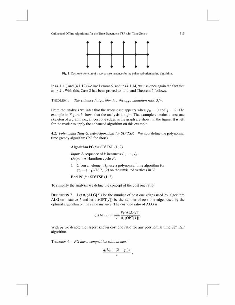
Fig. 5. Cost one skeleton of a worst case instance for the enhanced orienteering algorithm.

In (4.1.11) and (4.1.12) we use Lemma 9, and in (4.1.14) we use once again the fact thatk0 ≥ k1. With this, Case 2 has been proved to hold, and Theorem 5 follows.

THEOREM 5. The enhanced algorithm has the approximation ratio 3/4.

From the analysis we infer that the worst-case appears when p0 = 0 and j = 2. Theexample in Figure 5 shows that the analysis is tight. The example contains a cost oneskeleton of a graph, i.e., all cost one edges in the graph are shown in the figure. It is leftfor the reader to apply the enhanced algorithm on this example.

4.2. Polynomial Time Greedy Algorithms for SDkTSP. We now define the polynomialtime greedy algorithm (PG for short).

Algorithm PG for SDkTSP (1, 2)


1 Given an element Ij , use a polynomial time algorithm for(zj − zj−1)-TSP(1,2) on the unvisited vertices in V .

End PG for SDkTSP (1, 2)

To simplify the analysis we define the concept of the cost one ratio.

DEFINITION 7. Let #1(ALG[I ]) be the number of cost one edges used by algorithmALG on instance I and let #1(OPT[I ]) be the number of cost one edges used by theoptimal algorithm on the same instance. The cost one ratio of ALG is

q1(ALG) = minI

#1(ALG[I ])

#1(OPT[I ]).

With q1 we denote the largest known cost one ratio for any polynomial time SDkTSPalgorithm.

THEOREM 6. PG has a competitive ratio at most

q1Uk + (2− q1)n

n.


PROOF. Let PI denote the cycle produced by the new greedy algorithm. In every timezone the number of cost one edges used by PG is at least q1 times the number of costone edges used by OPT that were not counted by the usage function.

This adds up to

2Uk(PI )+ q1(n −Uk(PI ))+ 2(1− q1)(n −Uk(PI ))

n

= q1Uk(PI )+ (2− q1)n

n≤ q1Uk + (2− q1)n

n.

We can adopt the enhanced orienteering algorithm in the previous section to get ak-TSP path algorithm with q1 = 2

3 by returning a path of length T instead of a path withcost T . (To see that the algorithm attains this cost one ratio it is sufficient to considerits worst case, in which every third edge in the path has cost two when all edges in theoptimal path have cost one.) Using PG with this new algorithm as a subroutine we getthe competitive ratio

23Uk + 4

3 n

n.

Using the results in Theorem 2 we get the following largest competitive ratio:

2(2k − 2)

3(2k − 1)+ 4

3.

We present the competitive ratios for some values of k in Table 1.Not surprisingly these values are rather close to 2. Note that the only cost one edges

we can hope for in the worst case lie in time zone one. This situation does not changewith a better orienteering algorithm. Thus, to improve the approximation ratio we need tomodify the polynomial time greedy algorithm. We call the new algorithm IPG (improvedgreedy).

Algorithm IPG for SDkTSP(1, 2)


1 Use PG on every permutation of the set {I1, . . . , Ik}, and return thecheapest solution.

End IPG for SDkTSP(1, 2)

To measure the performance of this algorithm we note that no offline algorithm cansimultaneously force a value on the corresponding usage function U ′k higher than

U ′k = minπ{U (Aπ )},

where π is a permutation of {1, . . . , k} and Aπ is the polynomial time greedy algorithmusing the input sequence Iπ1 , Iπ2 , . . . , Iπk . A trivial upper bound on U ′k is if zj = jn/k,


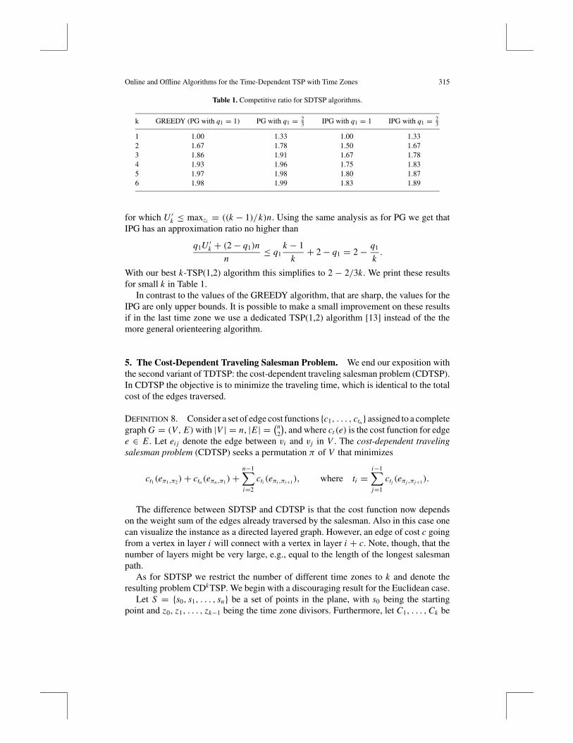
Table 1. Competitive ratio for SDTSP algorithms.

k GREEDY (PG with q1 = 1) PG with q1 = 23 IPG with q1 = 1 IPG with q1 = 2

3

1 1.00 1.33 1.00 1.332 1.67 1.78 1.50 1.673 1.86 1.91 1.67 1.784 1.93 1.96 1.75 1.835 1.97 1.98 1.80 1.876 1.98 1.99 1.83 1.89

for which U ′k ≤ maxzi = ((k − 1)/k)n. Using the same analysis as for PG we get thatIPG has an approximation ratio no higher than

q1U ′k + (2− q1)n

n≤ q1

k − 1

k+ 2− q1 = 2− q1

k.

With our best k-TSP(1,2) algorithm this simplifies to 2 − 2/3k. We print these resultsfor small k in Table 1.

In contrast to the values of the GREEDY algorithm, that are sharp, the values for theIPG are only upper bounds. It is possible to make a small improvement on these resultsif in the last time zone we use a dedicated TSP(1,2) algorithm [13] instead of the themore general orienteering algorithm.

5. The Cost-Dependent Traveling Salesman Problem. We end our exposition withthe second variant of TDTSP: the cost-dependent traveling salesman problem (CDTSP).In CDTSP the objective is to minimize the traveling time, which is identical to the totalcost of the edges traversed.

DEFINITION 8. Consider a set of edge cost functions {c1, . . . , ctn } assigned to a completegraph G = (V, E)with |V | = n, |E | = (n

2

), and where ct (e) is the cost function for edge

e ∈ E . Let ei j denote the edge between vi and vj in V . The cost-dependent travelingsalesman problem (CDTSP) seeks a permutation π of V that minimizes

ct1(eπ1,π2)+ ctn (eπn ,π1)+n−1∑

i=2

cti (eπi ,πi+1), where ti =i−1∑

j=1

ctj (eπj ,πj+1).

The difference between SDTSP and CDTSP is that the cost function now dependson the weight sum of the edges already traversed by the salesman. Also in this case onecan visualize the instance as a directed layered graph. However, an edge of cost c goingfrom a vertex in layer i will connect with a vertex in layer i + c. Note, though, that thenumber of layers might be very large, e.g., equal to the length of the longest salesmanpath.

As for SDTSP we restrict the number of different time zones to k and denote theresulting problem CDkTSP. We begin with a discouraging result for the Euclidean case.

Let S = {s0, s1, . . . , sn} be a set of points in the plane, with s0 being the startingpoint and z0, z1, . . . , zk−1 being the time zone divisors. Furthermore, let C1, . . . ,Ck be


k positive values such that C1 < · · · < Ck . We define the function

C(t) = Ci if τi−1 ≤ t < τi for 1 ≤ i ≤ k.

Consider a salesman that visits the points in S. We define the departure time ti of point si

as the point in time when the salesman leaves point si .The Restricted Euclidean CDTSP is the problem of finding a tour that visits all the

points in S, minimizing the total traveling time. The time needed to go between twopoints si and sj is given by d(si , sj )C(ti ), where d(si , sj ) is the distance between the twopoints. We assume that the departure time of the starting point is t0 = z0 = 0.

Garey et al. [8] prove that the Euclidean traveling salesman problem is NP-hardby a reduction from the NP-complete decision problem exact cover by 3-sets, X3C.We use their reduction to prove that the Restricted Euclidean CDTSP is inapproximable.If F is a yes instance of X3C, then we say that F ∈ X3C, otherwise we say thatF �∈ X3C.

Let S be an instance of TSP produced by Garey et al.’s reduction, such that |S| = n.The points of S lie on a unit grid G of size less that n×n and a naive tour visiting all pointsof S has a cost l < 2n. These results follow directly from Garey et al.’s construction.

Garey et al. prove that the cost of an optimal tour is less than or equal to some specificvalue L∗ if an exact cover exists for the X3C instance. If there is no exact cover, then ithas at least the cost L∗+1.

THEOREM 7. The Euclidean CD2TSP cannot be approximated by any constant factor.

PROOF. We construct a Restricted Euclidean CDTSP instance based upon the instanceused in the reduction of Garey et al. Let r be an arbitrary constant. We take S fromthe reduction of Garey et al. as the set of points in the Restricted Euclidean CDTSPinstance, with the lower leftmost point as the depot. We let z0 = 0, z1 = L∗, C1 = 1,and C2 = (r−1)L∗.

If F ∈ X3C, then the time needed by an optimal salesman to visit all points andgo back to the depot is L∗ as in the TSP instance of Garey et al. On the other hand, ifF �∈ X3C, then the cost of the optimal tour in the TSP instance is at least L∗+1. Theshortest Hamilton path starting from the lower leftmost point is therefore at least L∗

long. For the Restricted Euclidean CDTSP instance this implies that the departure timeof the last point si to be visited by the salesman is at least L∗. The cost of the last edgeis therefore (r−1)L∗d(si , s0) ≥ (r−1)L∗, since d(si , s0) ≥ 1. The total traveling timeis thus at least r L∗ and the approximation ratio becomes at least r L∗/L∗ = r . Since wecan choose r arbitrarily large, the theorem follows.

We again restrict the edge costs to either one or two and consider the online versionof CD2TSP. Once again the greedy algorithm is optimal.

THEOREM 8. The competitive ratio of online CD2TSP(1, 2) is 5/3 and the greedy al-gorithm is optimal.

We give two lemmas that together give us the proof of Theorem 8.


LEMMA 10. The competitive ratio of any online algorithm for CD2TSP(1, 2) with twotime zones is at least 5/3.

PROOF. Let z1 = n/3 and assume that each edge in time zone one has cost one. Takean arbitrary online algorithm ALG for this problem and consider its performance. Thealgorithm must produce an initial path of cost and length n/3 before acquiring the costof the edges in time zone two. The adversary makes sure that ZIG[1] and ALG[1] aredisjoint and that all edges incident to black vertices get cost one in time zone two. Allother edges get cost two. Since the only edges with cost one in time zone two are thoseincident to vertices already visited by ALG, the cost of time zone two is 4n/3 and thetotal cost of the tour is 5n/3. ZIG can use all cost one edges in time zone two and achievethe total cost n, since ZIG[1] and ALG[1] are disjoint.

Below, we present an optimal exponential-time online algorithm for CD2TSP(1, 2)withtwo time zones. The input to the algorithm is the cost matrix for time zone one and attime z1 the algorithm is given the cost function of time zone two.

Algorithm Aexp

1 Compute the longest path of cost ≤ z1.2 Get new input (new cost function).3 Compute the min cost path from the current position to the starting

point.

End Aexp

LEMMA 11. Aexp has competitive ratio 5/3.

PROOF. Let m1 be the number of edges in the tour produced by Aexp, restricted to timezone one, and let Aexp(I2) be the cost of the tour restricted to time zone two. Furthermore,let m2 and OPT(I2) be the corresponding variables for the optimal tour. The competitiveratio of Aexp can be expressed as

R(Aexp) = z1 + Aexp(I2)

z1 + OPT(I2).

The cost one edges that can be used by an offline algorithm but not by the onlinealgorithm are the edges in time zone two that are incident to black vertices. The maximalnumber of such edges included in a tour is min{2m1, n−m2}. The rest of the edges usedby the offline algorithm in the second time zone may also be used by Aexp. These edgesconnect a number of vertices that both tours visit in this time zone. If we let opt denote theshortest TSP path among these vertices, we get that OPT(I2) ≥ min{2m1, n−m2}+opt .

We apply the same argument for the cost two edges in time zone two. The cost twoedges that Aexp’s tour may be forced to visit but that the optimal tour may escape arethe edges that are adjacent to vertices already visited by the optimal tour. The maximalnumber of such edges in Aexp’s tour is min{2m2, n − m1}, and since Aexp computes an


optimal TSP path in time zone two, it follows that Aexp(I2) ≤ 2 min{2m2, n−m1}+opt .Since m2 ≤ m1 it follows that the competitive ratio is

R(Aexp) ≤ z1 + 2 min{2m1, n − m1} + opt

z1 +min{2m1, n − m1} + opt= 1+ min{2m1, n − m1}

z1 +min{2m1, n − m1} + opt.

This ratio is maximized for m1 = n/3 for which opt = 0, and since z1 ≥ m1, we getthat

R(Aexp) ≤ 1+ 2n/3

n/3+ 2n/3= 5

3.

Using the improved greedy algorithm for CD2TSP we can achieve the same approx-imation ratio in polynomial time.

COROLLARY 3. There is a polynomial time offline 5/3-approximation algorithm forCD2TSP(1, 2).

Note that we achieve the same result as for the two time zone SDTSP. However,because of the increased complexity in the dependency between time and cost we arenot able to generalize the result to hold for k time zones.

6. Conclusions. We study online strategies for two versions of the time-dependenttraveling salesman problem (SDkTSP and CDkTSP).

For the online version of SDkTSP we achieve an optimal exponential time strategywith competitive ratio (M/m − 1)((2k − 2)/(2k − 1))+ 1, where M is the largest andm the smallest edge cost, and k is the number of time zones.

In order to make the online strategy time efficient we study the orienteering problem,which appears as a subproblem in the online strategy. We find an approximation algorithmfor the orienteering problem with approximation ratio 3/4 if the edge costs are restrictedto one and two.

Using the online result for SDkTSP together with the approximation algorithm forthe orienteering problem we are able to produce a greedy approximation algorithm withapproximation factor 2 − 2/3k for graphs with edge costs one or two. We also givesimilar results for CD2TSP(1, 2), matching those found for SD2TSP(1, 2).

References

[1] E. M. Arkin, G. Narasimhan, and J. S. B. Mitchell. Resource-constrained geometric network optimiza-tion. In Proc. Fourteenth ACM Symposium on Computational Geometry, pages 307–316, 1998.

[2] G. Ausiello, E. Feuerstein, S. Leonardi, L. Stougie, and M. Talamo. Algorithms for the on-line travelingsalesman. Algorithmica, 29(4):560–581, 2001.

[3] N. Balakrishnan, A. Lucena, and R. T. Wong. Scheduling examinations to reduce second-order conflicts.Computers in Operations Research, 19:353–361, 1992.

[4] M. Blom, S. O. Krumke, W. de Paepe, and L. Stougie. The online-TSP against fair adversaries. InAlgorithms and Complexity: 4th Italian Conference, CIAC 2000, pages 137–149. Lecture Notes inComputer Science, 1767. Springer-Verlag, Berlin, 2000.


[5] K. Fox. Production Scheduling on Parallel Lines with Dependencies. Ph.D. thesis, The Johns HopkinsUniversity, Baltimore, MD, 1973.

[6] K. Fox, B. Gavish, and S. Graves. An n-constraint formulation of the (time-dependent) travelingsalesman problem. Operations Research, 28:1018–1021, 1980.

[7] H. N. Gabow. Data structures for weighted matching and nearest common ancestors with linking. InProc. 1st Annual ACM–SIAM Symposium on Discrete Algorithms, pages 434–443, 1990.

[8] M. R. Garey, R. L. Graham, and D. S. Johnson. Some NP-complete geometric problems. In Proc. 8thAnnual ACM Symposium on Theory of Computing, pages 10–21, 1976.

[9] M. Hammar and B. J. Nilsson. Approximation results for kinetic variants of TSP. In Proc. ICALP,pages 392–401, 1999.

[10] C. S. Helvig, G. Robins, and A. Zelikovsky. Moving-target TSP and related problems. In Proc. 6thAnnual European Symposium on Algorithms (ESA), pages 453–464, 1998.

[11] M. Lipmann. The Online Traveling Salesman Problem on the Line. Master’s thesis, Department ofOperations Research, University of Amsterdam, 1999.

[12] C. Malandraki and M. S. Daskin. Time dependent vehicle routing problems: formulations, propertiesand heuristic algorithms. Transportation Science, 26:185–200, 1992.

[13] C. H. Papadimitriou and M. Yannakakis. The traveling salesman problem with distances one and two.Mathematics of Operations Research, 18(1):1–11, 1993.

[14] J. C. Picard and M. Queyranne. The time-dependent traveling salesman problem and its application tothe tardiness problem in one machine scheduling. Operations Research, 26:86–110, 1978.

Documents

Online and Offline Algorithms for the Time-Dependent TSP with Time Zones