Online Algorithms for Market Clearing∗

Avrim Blum†

Tuomas Sandholm†

Martin Zinkevich†

Abstract

In this paper we study the problem of online market clearing where there is one commodity inthe market being bought and sold by multiple buyers and sellers whose bids arrive and expire atdifferent times. The auctioneer is faced with an online clearing problem of deciding which buyand sell bids to match without knowing what bids will arrive in the future. For maximizing profit,we present a (randomized) online algorithm with a competitive ratio of ln(pmax−pmin)+1, whenbids are in a range [pmin, pmax], which we show is the best possible. A simpler algorithm has aratio twice this, and can be used even if expiration times are not known. For maximizing thenumber of trades, we present a simple greedy algorithm that achieves a factor of 2 competitiveratio if no money-losing trades are allowed. We also show that if the online algorithm is allowedto subsidize matches — match money-losing pairs if it has already collected enough money fromprevious pairs to pay for them — then it can actually be 1-competitive with respect to theoptimal offline algorithm that is not allowed subsidy. That is, the ability to subsidize is at leastas valuable as knowing the future. We also consider objectives of maximizing buy or sell volumeand social welfare. We present all of these results as corollaries of theorems on online matchingin an incomplete interval graph.

We also consider the issue of incentive compatibility, and develop a nearly optimal incentive-compatible algorithm for maximizing social welfare. For maximizing profit, we show that noincentive-compatible algorithm can achieve a sublinear competitive ratio, even if only one buybid and one sell bid are alive at a time. However, we provide an algorithm that, under certainmild assumptions on the bids, performs nearly as well as the best fixed pair of buy and sellprices, a weaker but still natural performance measure. This latter result uses online learningmethods, and we also show how such methods can be used to improve our “optimal” algorithmsto a broader notion of optimality. Finally, we show how some of our results can be generalizedto settings in which the buyers and sellers themselves have online bidding strategies, rather thanjust each having individual bids.

1 Introduction

Electronic commerce is becoming a mainstream mode of conducting business. In electronic com-merce there has been a significant shift to dynamic pricing via exchanges (that is, markets withpotentially multiple buyers and multiple sellers). The range of applications includes trading instock markets, bandwidth allocation in communication networks, as well as resource allocation inoperating systems and computational grids. In addition, exchanges play an increasingly importantrole in business-to-business commerce. Several independent business-to-business exchanges have

∗An extended abstract of this paper appeared in Proceedings of the 13th Annual Symposium on Discrete Algo-rithms (SODA) 2002. This paper contains additional results not present in the conference version.

†Computer Science Department, Carnegie Mellon University, Pittsburgh, PA 15213-3891.avrim,sandholm,maz@cs.cmu.edu

1

been founded (e.g., ChemConnect). In addition, large established companies have started to formbuying consortia such as Transora, Covisint, Exostar, Trade-Ranger, and Enporion. This sourcingtrend means that instead of one company buying from multiple suppliers, we have multiple com-panies buying from the multiple suppliers. In other words, sourcing is moving toward an exchangeformat.

These trends have led to an increasing need for fast market clearing algorithms for exchanges.Such algorithms have been studied in the offline (batch) context [25, 24, 26, 28]. Also, recent elec-tronic commerce server prototypes such as eMediator [23] and AuctionBot [27] have demonstrateda wide variety of new market designs, leading to the need for new clearing algorithms.

In this paper we study the ubiquitous setting where there is a market for one commodity, forexample, the stock of a single company, oil, electricity, memory chips, or CPU time, and clearingdecisions must be made online. For simplicity, we assume that each buy bid and each sell bid is fora single unit of the commodity (to buy or sell multiple units, a bidder could submit multiple bids1).In these settings, the auctioneer has to clear the market (match buy and sell bids) without knowingwhat the future buy/sell bids will be. The auctioneer faces the tradeoff of clearing all possiblesmatches as they arise versus waiting for additional buy/sell bids before matching. Waiting can leadto a better matching, but can also hurt because some of the existing buy/sell bids might expire orget retracted as the bidders get tired of waiting.

We formalize the problem faced by the auctioneer as an online problem in which buy and sellbids arrive over time. When a bid is introduced, the auctioneer learns the bid price and expirationtime (though some of the simpler algorithms will not need to know the expiration times). At anypoint in time, the auctioneer can match a live buy bid with a live sell bid, removing the pair fromthe system. We will also consider the problem both from the perspective of pure online algorithms— in which our goal is to design algorithms for the auctioneer whose performance is comparableto the best achievable in hindsight for the bid sequence observed — and from the perspective ofincentive-compatible mechanism design, in which we also are concerned that it be in the bidders’interests to actually bid their true valuations.

Note that while the Securities Exchange Commission imposes relatively strict rules on thematching process in securities markets like NYSE and NASDAQ [10], most new electronic markets(for example for business-to-business trading) are not securities markets. In those markets theauctioneer has significant flexibility in deciding which buy bids and sell bids to accept. In thispaper we will study how well the auctioneer can do in those settings, and with what algorithms.

1.1 Basic Definitions

We will assume that all bids and valuations are integer-valued (for example, that money cannot besplit more finely than pennies) and lie in some range [pmin, pmax].

Definition 1 A temporal clearing model consists of a set B of buy bids and a set S of sell bids.Each bid v ∈ B ∪ S has a positive price p(v), is introduced at a time ti(v), and removed at a timetf (v). A bid v is said to be alive in the interval [ti(v), tf (v)]. Two bids v, v′ ∈ B ∪ S are said to beconcurrent if there is some time when both are alive simultaneously.

1This works correctly if the buyers have diminishing marginal valuations for the units (the first unit is at leastas valuable as the second, etc.) and the sellers have increasing marginal valuations for the units. Otherwise, theauctioneer could allocate the bidder’s k + 1’st unit to the bidder without allocating the bidder’s k’th unit to thebidder, thus violating the intention of the bid by allocating a certain number of units to the bidder at a differentprice than the bidder intended. These restrictions seem natural—at least in the limit—as buyers get saturated andsellers run out of inventory and capacity to produce.

2

Definition 2 A legal matching is a collection of pairs (b1, s1), (b2, s2), . . . of buy and sell bidssuch that bi and si are concurrent.

An offline algorithm receives knowledge of all buy and sell bids up front. An online algorithmonly learns of bids when they are introduced. Both types of algorithms have to produce a legalmatching: that is, a buy bid and sell bid can only be matched if they are concurrent. In ourbasic model, if the algorithm matches buy bid b with sell bid s (buying from the seller and sellingto the buyer), it receives a profit of p(b) − p(s). We will use competitive analysis [7] to measurethe quality of an online algorithm, comparing its performance (in expectation, if the algorithm israndomized) on a bid sequence to that of the optimal offline solution for the same sequence. Notethat in this measure we do not worry that had we acted differently, we might have seen a bettersequence of bids: the comparison is only to the optimum on the sequence observed. Formally, thecompetitive ratio of an algorithm is the worst-case, over all possible bid sequences, of the ratio ofits performance to the optimal offline solution on that sequence. We will consider several measuresof “performance”, including total profit, number of trades, and social welfare (see Section 1.3).

In Section 5.2 we consider a generalization of the temporal clearing model in which bidders canchange their bids over time. In this generalization, each bid can be a function of time, with onlythe values so far revealed to the online algorithm, and the goal of the algorithm is to be competitivewith the optimal offline solution for the actual functions.

The basic competitive-analysis model implicitly treats bidders as truthful in the sense that ittakes the bids as they come and compares to the offline optimum on the same bid sequence. This isa reasonable model in settings where the gaps between buy and sell bids are fairly small comparedto the prices themselves, and where true valuations are difficult to quantify (e.g., say in a stockmarket). However, we also consider in Section 6 the more general model of incentive-compatiblemechanism design, in which we assume each bidder has a private valuation for the commodity, andour goal is to compete with respect to the optimal offline solution for the actual valuations of allthe bidders. In this context, the mechanism must give bidders reason to bid their true valuations.We assume (though we relax this for some of our results) that the start and end times for bids arenot manipulable: the only control agents have is over their bid values. Even this, however, providesa sharp contrast between the setting of exchanges, which we consider here, and the simpler case ofauctions.

1.2 Auctions versus Exchanges

Competitive analysis of auctions (multiple buyers submitting bids to one seller) has been conductedby a number of authors [2, 3, 6, 13, 14, 19]. In this paper, we present the first competitive analysisof online exchanges (where there can be multiple buyers and multiple sellers submitting bids overtime). Competitive analysis of 1-shot exchanges (all bids concurrent) has been performed in [9].Exchanges are a generalization of auctions — one could view an exchange as a number of overlappingauctions — and they give rise to additional issues. For example, if a seller does not accept a buybid, some other seller might.

There are two primary differences between auctions and exchanges with respect to the designof algorithms. The first is that in addition to the basic question of what profit threshold to requireper sale, for exchanges there is the additional complication of deciding which bids meeting thatcriterion one should in fact match (e.g., maximizing the number of profitable trades is trivial for anauction). So achieving an optimal competitive ratio will require performing both tasks optimally. Asecond more subtle distinction, however, which impacts issues of incentive-compatibility, concerns

3

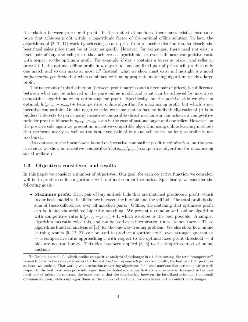
the relation between prices and profit. In the context of auctions, there must exist a fixed salesprice that achieves profit within a logarithmic factor of the optimal offline solution (in fact, thealgorithms of [2, 7, 11] work by selecting a sales price from a specific distribution, so clearly thebest fixed sales price must be at least as good). However, for exchanges, there need not exist afixed pair of buy and sell prices that achieves a logarithmic, or even sublinear competitive ratiowith respect to the optimum profit. For example, if day i contains a buyer at price i and seller atprice i + 1, the optimal offline profit in n days is n, but any fixed pair of prices will produce onlyone match and so can make at most 1.2 Instead, what we show must exist in hindsight is a goodprofit margin per trade that when combined with an appropriate matching algorithm yields a largeprofit.

The net result of this distinction (between profit margins and a fixed pair of prices) is a differencebetween what can be achieved in the pure online model and what can be achieved by incentive-compatible algorithms when optimizing for profit. Specifically, on the positive side we give anoptimal, ln(pmax − pmin) + 1-competitive, online algorithm for maximizing profit, but which is notincentive-compatible. On the negative side, we show that in fact no individually-rational (it is inbidders’ interests to participate) incentive-compatible direct mechanism can achieve a competitiveratio for profit sublinear in pmax−pmin, even in the case of just one buyer and one seller. However, onthe positive side again we present an incentive-compatible algorithm using online learning methodsthat performs nearly as well as the best fixed pair of buy and sell prices, so long as traffic is nottoo bursty.

(In contrast to the linear lower bound on incentive compatible profit maximization, on the pos-itive side, we show an incentive compatible 2 ln(pmax/pmin)-competitive algorithm for maximizingsocial welfare.)

1.3 Objectives considered and results

In this paper we consider a number of objectives. Our goal, for each objective function we consider,will be to produce online algorithms with optimal competitive ratios. Specifically, we consider thefollowing goals:

• Maximize profit. Each pair of buy and sell bids that are matched produces a profit, whichin our basic model is the difference between the buy bid and the sell bid. The total profit is thesum of these differences, over all matched pairs. Offline, the matching that optimizes profitcan be found via weighted bipartite matching. We present a (randomized) online algorithmwith competitive ratio ln(pmax − pmin) + 1, which we show is the best possible. A simpleralgorithm has ratio twice this, and can be used even if expiration times are not known. Thesealgorithms build on analysis of [11] for the one-way-trading problem. We also show how onlinelearning results [5, 12, 21] can be used to produce algorithms with even stronger guarantees— a competitive ratio approaching 1 with respect to the optimal fixed profit threshold — ifbids are not too bursty. This idea has been applied [3, 6] to the simpler context of onlineauctions.

2In Deshmukh et al. [9], which studies competitive analysis of exchanges in a 1-shot setting, the term “competitive”is used to refer to the ratio with respect to the best fixed pair of buy/sell prices (technically, the best pair that producesat least two trades). That work gives a reduction converting algorithms for 1-shot auctions that are competitive withrespect to the best fixed sales price into algorithms for 1-shot exchanges that are competitive with respect to the bestfixed pair of prices. In contrast, the issue here is that the relationship between the best fixed price and the overalloptimum solution, while only logarithmic in the context of auctions, becomes linear in the context of exchanges.

4

In Section 6, we consider the issue of incentive-compatible mechanism design, where weprove both a negative result and a positive result. On the negative side, we show no direct,individually rational, incentive-compatible mechanism can achieve a competitive ratio thatis sublinear in pmax − pmin. On the positive side, however, we give an incentive-compatiblealgorithm that performs well with respect to the best fixed pair of buy and sell prices (sublinearadditive regret so long as bids are not too bursty) using online learning techniques.

• Maximize liquidity. Liquidity maximization is important for a marketplace for severalreasons. The success and reputation of an electronic marketplace is often measured in termsof liquidity, and this affects the (acquisition) value of the party that runs the marketplace.Also, liquidity attracts buyers and sellers to the marketplace; after all, they want to be ableto buy and sell.

We analyze three common measures of liquidity: 1) number of trades, 2) sum of the pricesof the cleared buy bids (buy volume), and 3) sum of the prices of the cleared sell bids (sellvolume). Under criterion 1, the goal is to maximize the number of trades made, rather thanthe profit, subject to not losing money. We show that a simple greedy algorithm achieves afactor of 2 competitive ratio, if no money-losing trades are allowed. This can be viewed asa variant on the on-line bipartite matching problem [17]. Interestingly, we show that if theonline algorithm is allowed to subsidize matches — match money-losing pairs if it has alreadycollected enough money from previous pairs to pay for them — then it can be 1-competitivewith respect to the optimal offline algorithm that is not allowed subsidy. That is, the abilityto subsidize is at least as valuable as knowing the future. (If the offline algorithm can alsosubsidize then no finite competitive ratio is possible).

For the problems of maximizing buy or sell volume, we present algorithms that achieve acompetitive ratio of 2(ln(pmax/pmin) + 1) without subsidization. We also present algorithmsthat achieve a competitive ratio of ln(pmax/pmin) + 1 with subsidization with respect to theoptimal offline algorithm that cannot use subsidies. This is the best possible competitiveratio for this setting.

• Maximize social welfare. This objective corresponds to maximizing the good of the buyersand sellers in aggregate. Specifically, the objective is to have the items end up in the handsof the agents that value them the most. We obtain an optimal competitive ratio, which isthe fixed point of the equation r = ln pmax

(r−1)pmin. Using an incentive-compatible algorithm, we

can achieve a competitive ratio at most twice this.

We develop all of our best algorithms in a more general setting we call the incomplete interval-graph matching problem. In this problem, we have a number of intervals (bids), some of whichoverlap in time, but only some of those may actually be matched (because we can only match a buyto a sell, because the prices must be in the correct order, etc.). By addressing this more generalsetting, we are able to then produce our algorithmic results as corollaries.

2 An Abstraction: Online Incomplete Interval Graphs

In this section we introduce an abstraction of the temporal bidding problem that will be useful forproducing and analyzing optimal algorithms, and may be useful for analyzing other online problemsas well.

5

Definition 3 An incomplete interval graph is a graph G = (V,E), together with two functions tiand tf from V to [0,∞) such that:

1. For all v ∈ V , ti(v) < tf (v).

2. If (v, v′) ∈ E, then ti(v) ≤ tf (v′) and ti(v′) ≤ tf (v).

We call ti(v) the start time of v, and tf (v) the expiration time of v. For simplicity, we assume thatfor all v 6= v′ ∈ V , ti(v) 6= ti(v

′) and tf (v) 6= tf (v′).3

An incomplete interval graph can be thought of as an abstraction of the temporal biddingproblem where we ignore the fact that bids come in two types (buy and sell) and have pricesattached to them, and instead we just imagine a black box “E” that given two bids v, v′ thatoverlap in time, outputs an edge if they are allowed to be matched. By developing algorithms forthis generalization first, we will be able to more easily solve the true problems of interest.

We now consider two problems on incomplete interval graphs: the online edge-selection problemand the online vertex-selection problem. In the online edge-selection problem, the online algorithmmaintains a matching M . The algorithm sees a vertex v at the time it is introduced (that is, attime ti(v)). At this time, the algorithm is also told of all edges from v to other vertices which havealready been introduced. The algorithm can select an edge only when both endpoints of the edgeare alive. Once an edge has been selected, it can never be removed. The objective is to maximizethe number of edges in the final matching, |M |.

In the online vertex-selection problem, the online algorithm maintains a set of vertices W , withthe requirement that there must exist some perfect matching on W . At any point in time, thealgorithm can choose two live vertices v and v′ and add them into W so long as there exists aperfect matching on W ∪ v, v′. Note that there need not exist an edge between v and v′. Theobjective is to maximize the size of W . So, the vertex-selection problem can be thought of as a lessstringent version of the edge-selection problem in that the algorithm only needs to commit to theendpoints of the edges in its matching, but not the edges themselves.

It is easy to see that no deterministic online algorithm can achieve a competitive ratio less than2 for the edge-selection problem.4 A simple greedy algorithm achieves this ratio:

Algorithm 1 (Greedy) When a vertex is introduced, if it can be matched, match it (to any oneof the vertices to which it can be matched).

The fact that Greedy achieves a competitive ratio of 2 is essentially folklore (e.g., this fact ismentioned in passing for a related model in [17]). For completeness, we give the proof here.

Theorem 1 The Greedy algorithm achieves a competitive ratio of 2 for the edge-selection problem.

Proof: Consider an edge (v, v′) in the optimal matching M∗. Define v to be the vertex which isintroduced first, and v′ to be the vertex which is introduced second. Then the algorithm will matcheither v or v′. In particular, if v is not matched before v′ is introduced, then we are guaranteed v′

3All our results can be extended to settings without this restriction, and where ti(v) may equal tf (v). This isaccomplished by imposing an artificial total order on simultaneous events. Among the events that occur at any giventime, bid introduction events should precede bid expiration events. The introduction events can be ordered, forexample, in the order they were received, and so can the expiration events.

4Consider the following scenario: vertex u expires first and has edges to v1 and v2. Then, right after u expires, anew vertex w arrives with an edge to whichever of v1 or v2 the algorithm matched to u.

6

will be matched (either to v or some other vertex). Therefore, the number of vertices in the onlinematching M is at least the number of edges in M∗, which means |M | ≥ |M∗|/2.

For the vertex-selection problem, we show the following algorithm achieves a competitive ratio of1. That is, it is guaranteed to find (the endpoints of) a maximum matching in G.

Algorithm 2 Let W be the set of vertices selected so far by the algorithm. When a vertex v isabout to expire, consider all the live unmatched vertices v′, sorted by expiration time from earliestto latest. Add the first pair v, v′ to W such that there exists a perfect matching on W ∪ v, v′.Otherwise, if no unmatched vertex v′ has this property, allow v to expire unmatched.

Theorem 2 (Main Theorem) Algorithm 2 produces a set of nodes having a perfect matching Mwhich is a maximum matching in G.

The proof of Theorem 2 appears in Appendices A and B. The core of the proof is to show thatif W is the set of selected vertices, then at all times the following invariants hold:

H1: For any expired, unmatched vertex w, there does not exist any untaken vertex w′ such thatthere is a perfect matching on W ∪ w,w′. (An untaken vertex is a vertex that has beenintroduced but not matched.)

H2: For any matched vertex w, there does not exist an untaken vertex w′ such that there is aperfect matching on W ∪ w′ − w and tf (w) > tf (w′).

H3: For any two unexpired vertices w,w′ ∈W , there exists no perfect matching on W − w,w′.

The first invariant says that the algorithm is complete: it lets no matchable vertex expire, andexpired vertices do not later become matchable. The second and third invariants say that thealgorithm is cautious. The second invariant says that the algorithm favors vertices which expireearlier over those which expire later. The third invariant states that the algorithm only matchesvertices that it has to: no subset of the set of vertices chosen has a perfect matching and containsall of the expired vertices5.

Since an untaken vertex is a vertex which has been introduced but not matched, no untakenvertices exist at the start of the algorithm. Also, W is empty. Therefore, these invariants vacuouslyhold at the start.

Three events can occur: a vertex is introduced, a vertex expires without being matched, or avertex expires and is added with some other vertex to W . We establish that if all the invariantshold before any of these events, then they hold afterwards as well. If the first invariant holds atthe termination of the algorithm, then no pair could be added to the set selected. The augmentingpath theorem [4] establishes that the selected set is therefore optimal. See Appendices A and B fora full proof.

3 Competitive Algorithms for Profit, Liquidity, and Welfare

We now show how the results of Section 2 can be used to design optimal algorithms for the temporalbidding problem for the objectives of maximizing profit, liquidity, and social welfare. In each case,

5The paraphrasing of this last point is a bit more extreme than the others, but it turns out that if there exists aperfect matching on W and a perfect matching on W ′ ⊂ W , then there exists two vertices v, v′ ∈ W −W ′ such thatthere is a perfect matching on W − v, v′.

7

we construct a graph in which vertices are bids and edges are placed between a buy bid and asell bid if they overlap and meet some additional criteria (such as having a price gap of at leastsome threshold θ) that will depend on the specific problem. Note that because bids are intervals,if Algorithm 2 chooses to add some pair v, v′ to its matching, the corresponding bids will overlapin time, even though there may not be a direct edge between them in the graph.

3.1 Profit Maximization

We now return to the temporal bidding problem and show how the above results can be used toachieve an optimal competitive ratio for maximizing profit.

We can convert the profit maximization problem to an incomplete interval graph problem bychoosing some θ to be the minimum profit which we will accept to match a pair. So, when translatingfrom the temporal bidding problem to the incomplete interval matching problem, we insert an edgebetween a concurrent buy bid b and a sell bid s if and only if p(b) ≥ p(s) + θ.

The Greedy algorithm (Algorithm 1) then corresponds to the strategy: “whenever there existsa pair of bids in the system that would produce a profit at least θ, match them immediately.”Algorithm 2 attempts to be more sophisticated: first of all, it waits until a bid is about to expire,and then considers the possible bids to match to in order of their expiration times. (So, unlikeGreedy, this algorithm needs to know what the expiration times are.) Second, it can choose tomatch a pair with profit less than θ if the actual sets of matched buy and sell bids could have beenpaired differently in hindsight so as to produce a matching in which each pair yields a profit of atleast θ. This is not too bizarre since the sum of surpluses is just the sum of buy prices minus thesum of sell prices, and so does not depend on which was matched to which.

Define M∗(Gθ) to be the maximum matching in the incomplete interval graph Gθ produced inthe above manner. Then, from Theorem 1, the greedy edge-selection algorithm achieves a profit ofat least 1

2θ · |M∗(Gθ)|. Applying Algorithm 2 achieves surplus of at least θ · |M∗(Gθ)|.The final issue is how we choose θ. If we set θ to 1, then the number of matched pairs will be

large, but each one may produce little surplus. If we set θ deterministically any higher than 1, it ispossible the algorithms will miss every pair, and have no surplus even when the optimal matchinghas surplus. Instead, one approach is to use Classify-and-Randomly-Select [20, 1]: choose θ = 2i

for i chosen at random from 0, 1, . . . , ` for ` = blg(pmax − pmin)c. In this case, in expectationa 1/(` + 1) fraction of OPT’s profit is from matches made between bids whose prices differ by anamount in the range [θ, 2θ], and therefore the expected value of θ ·|M∗(Gθ)| is at least 1

2OPT/(`+1).We can achieve a tighter bound by choosing an exponential distribution as in in [11] (see also [15]).Specifically, for all x ∈ [1, pmax − pmin], let

Pr[θ ≤ x] =ln(x) + 1

ln(pmax − pmin) + 1,

where Pr[θ = 1] = 1ln(pmax−pmin)+1 . Observe that this is a valid probability distribution. Let OPT

be the surplus achieved by the optimal offline algorithm.

Lemma 1 If θ is chosen from the above distribution, then E[θ · |M∗(Gθ)|] ≥OPT

ln(pmax−pmin)+1 .

Corollary 1 The algorithm that chooses θ from the above distribution and then applies Greedyto the resulting graph achieves competitive ratio 2(ln(pmax − pmin) + 1). Replacing Greedy withAlgorithm 2 achieves competitive ratio ln(pmax − pmin) + 1.

8

In Section 4 we prove a corresponding lower bound of ln(pmax − pmin) + 1 for this problem.Proof (of Lemma 1): Let us focus on a specific pair (b, s) matched by OPT. Let Rθ(b, s) = θ ifp(b)−p(s) ≥ θ and Rθ(b, s) = 0 otherwise. Observe that θ · |M∗(Gθ)| ≥

∑

(b,s)∈OPT Rθ(b, s) becausethe set of pairs of profit at least θ matched by OPT is a legal matching in the incomplete intervalgraph. So, it suffices to prove that E[Rθ(b, s)] ≥ (p(b)− p(s))/(ln(pmax − pmin) + 1).

We do this as follows. First, for x > 1, ddx Pr[θ ≤ x] = 1

x(ln(pmax−pmin)+1) . So,

E[Rθ(b, s)] = Pr[θ = 1] +

∫ p(b)−p(s)

1

xdx

x(ln(pmax − pmin) + 1)

=p(b)− p(s)

ln(pmax − pmin) + 1.

One somewhat strange feature of Algorithm 2 is that it may recommend matching a pair of buyand sell bids that actually have negative profit. Since this cannot possibly improve total profit,we can always just ignore those recommendations (even though the algorithm will think that wematched them).

3.2 Liquidity Maximization

In this section we study the online maximization of the different notions of liquidity: number oftrades, aggregate price of cleared sell bids, and aggregate price of cleared buy bids.

3.2.1 Maximizing the Number of Trades

Suppose that instead of maximizing profit, our goal is to maximize the number of trades made,subject to the constraint that each matched pair have non-negative profit. This can directly bemapped into the incomplete interval graph edge-matching problem by including an edge for everypair of buy and sell bids that are allowed to be matched together. So, the greedy algorithm achievescompetitive ratio of 2, which is optimal for a deterministic algorithm, as we prove in Section 4.3.

However, if the online algorithm can subsidize matches (match a pair of buy and sell bids ofnegative profit if it has already made enough money to pay for them) then we can use Algorithm 2,and do as well as the optimal solution in hindsight that is not allowed subsidization. Specifically,when Algorithm 2 adds a pair b, s to W , we match b and s together, subsidizing if necessary. Weknow that we always have enough money to pay for the subsidized bids because of the property ofAlgorithm 2 that its set W always has a perfect matching. We are guaranteed to do as well as thebest offline algorithm which is not allowed to subsidize, because the offline solution is a matchingin the incomplete interval graph. Thus, the ability to subsidize is at least as powerful as knowingthe future.6

3.2.2 Maximizing Buy or Sell Volume

A different important notion of liquidity is the aggregate size of the trades.

6If the offline algorithm is also allowed to subsidize money-losing matches, then no finite competitive ratio ispossible. In particular, if the offline algorithm can use knowledge of future profitable matches to subsidize money-losing matches in the present, then it is clear no interesting competitive ratio can be achieved; but even if the offlinealgorithm can only use past profits to subsidize, then the logarithmic lower bound on profit of Section 4.1 immediatelygives a corresponding lower bound for number of trades.

9

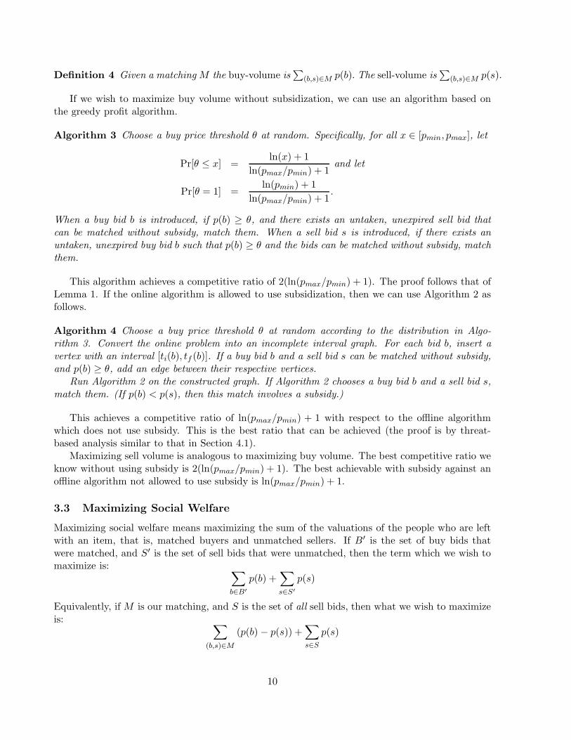
Definition 4 Given a matching M the buy-volume is∑

(b,s)∈M p(b). The sell-volume is∑

(b,s)∈M p(s).

If we wish to maximize buy volume without subsidization, we can use an algorithm based onthe greedy profit algorithm.

Algorithm 3 Choose a buy price threshold θ at random. Specifically, for all x ∈ [pmin, pmax], let

Pr[θ ≤ x] =ln(x) + 1

ln(pmax/pmin) + 1and let

Pr[θ = 1] =ln(pmin) + 1

ln(pmax/pmin) + 1.

When a buy bid b is introduced, if p(b) ≥ θ, and there exists an untaken, unexpired sell bid thatcan be matched without subsidy, match them. When a sell bid s is introduced, if there exists anuntaken, unexpired buy bid b such that p(b) ≥ θ and the bids can be matched without subsidy, matchthem.

This algorithm achieves a competitive ratio of 2(ln(pmax/pmin) + 1). The proof follows that ofLemma 1. If the online algorithm is allowed to use subsidization, then we can use Algorithm 2 asfollows.

Algorithm 4 Choose a buy price threshold θ at random according to the distribution in Algo-rithm 3. Convert the online problem into an incomplete interval graph. For each bid b, insert avertex with an interval [ti(b), tf (b)]. If a buy bid b and a sell bid s can be matched without subsidy,and p(b) ≥ θ, add an edge between their respective vertices.

Run Algorithm 2 on the constructed graph. If Algorithm 2 chooses a buy bid b and a sell bid s,match them. (If p(b) < p(s), then this match involves a subsidy.)

This achieves a competitive ratio of ln(pmax/pmin) + 1 with respect to the offline algorithmwhich does not use subsidy. This is the best ratio that can be achieved (the proof is by threat-based analysis similar to that in Section 4.1).

Maximizing sell volume is analogous to maximizing buy volume. The best competitive ratio weknow without using subsidy is 2(ln(pmax/pmin) + 1). The best achievable with subsidy against anoffline algorithm not allowed to use subsidy is ln(pmax/pmin) + 1.

3.3 Maximizing Social Welfare

Maximizing social welfare means maximizing the sum of the valuations of the people who are leftwith an item, that is, matched buyers and unmatched sellers. If B′ is the set of buy bids thatwere matched, and S′ is the set of sell bids that were unmatched, then the term which we wish tomaximize is:

∑

b∈B′

p(b) +∑

s∈S′

p(s)

Equivalently, if M is our matching, and S is the set of all sell bids, then what we wish to maximizeis:

∑

(b,s)∈M

(p(b)− p(s)) +∑

s∈S

p(s)

10

Note that the second term cannot be affected by the algorithm (because we assume that the bidsare predetermined). Furthermore, adding a constant to the offline and online algorithms’ objectivevalues can only improve the competitive ratio. Therefore, Corollary 1 immediately implies we canachieve a competitive ratio of ln(pmax − pmin) + 1. However, we can in fact do quite a bit better,using the following algorithm.

Algorithm 5 Let A be a given algorithm for matching on an incomplete interval graph with com-petitive ratio 1/α. Let r be the fixed point of the equation:

r =1

αln

pmax − pmin

(r − 1)pmin(1)

and let D be the (cumulative) distribution over [rpmin, pmax]:

D(x) =1

rαln

x− pmin

(r − 1)pmin(2)

The algorithm is as follows. Draw a threshold T such that Pr[T ≤ x] = D(x), and construct anincomplete interval graph by adding an edge between any concurrent pair of buy and sell bids b ands such that p(b) ≥ T and p(s) ≤ T . Then use algorithm A to perform the matching.

Theorem 3 Algorithm 5 has competitive ratio r from Equation 1. In particular, if Algorithm 2 isused as A, then the competitive ratio of Algorithm 5 is the fixed point of the equation:

r = lnpmax

(r − 1)pmin(3)

Note that this competitive ratio is at most max(2, ln(pmax/pmin)).

Theorem 4 The fixed point of Equation 3 is the optimal competitive ratio.

We prove Theorem 4 in Section 4.

Proof (of Theorem 3): The technique is similar to Lemma 1. First, let us associate utilitiesfrom trades with specific sell bids. Define S to be the set of sell bids. Fix an optimal matchingM∗. Let us define Ropt : S → [pmin, pmax] to be the valuation of the person who received the itemfrom seller s in the optimal matching. If s trades with b, then Ropt(s) = p(b). If s does not trade,then Ropt(s) = p(s). Observe that the optimal welfare is Wopt(s) =

∑

s∈S Ropt(s).For an arbitrary matching M , let us use the notation Mb,s(T ) to indicate the number of pairs

in M where the buy bid is greater than or equal to T and the sell bid is less than T . Similarly,define Mb,s(T ) to be the number of pairs in M where the buy bid and sell bid are both greaterthan or equal to T . Define Ms(T ) to be the number of unmatched sell bids greater than or equalto T . Recall that α is the reciprocal of the competitive ratio of the given matching algorithm A,and so is a lower bound on the fraction of potential trades actually harnessed.

Define N∗(T ) to be the number of agents (buyers and sellers) that end up with an item in theoptimal matching M∗, and have valuation greater than or equal to T . So,

N∗(T ) = |Ropt(s) ≥ T |s ∈ S| = M∗b,s(T ) + M∗

b,s(T ) + M∗s (T ).

11

Let Malg be a matching obtained by an online algorithm. Define Nalg(T ) to be the numberof agents (buyers and sellers) that end up with an item in the matching Malg, and have valuationgreater than or equal to T . Then,

Nalg(T ) ≥ αM∗b,s(T ) + M∗

b,s(T ) + M∗s (T ) ≥ α N∗(T ).

The social welfare achieved by the algorithm is at least

Nalg(T ) T + (|S| −Nalg(T ))pmin = (Nalg(T ))(T − pmin) + |S|pmin.

Because T > pmin, this is an increasing function of Nalg(T ), so the algorithm achieves social welfareat least

(α N∗(T ))(T − pmin) + |S|pmin.

Arithmetic manipulation yields

N∗(T )[αT + (1− α)pmin] + (|S| −N∗(T ))pmin.

By substitution we get

|Ropt(s) ≥ T |s ∈ S| [αT + (1− α)pmin] + |Ropt(s) < T |s ∈ S| pmin.

By defining RT (s) = αT +(1−α)pmin when Ropt(s) ≥ T and RT (s) = pmin otherwise, the algorithmis guaranteed to achieve social welfare of at least

∑

s∈S RT (s). We have divided the social welfare ona per sell bid basis. Therefore, if T is drawn according to D(x), we want to prove that E[RT (s)] ≥Ropt(s)

r for all s, the problem is solved. If Ropt(s) ≤ rpmin, then E[RT (s)] ≥ pmin ≥Ropt(s)

r . Considerthe case where Ropt(s) > rpmin. If T is drawn according to D(x), then since the density of T isD′(x) = 1

rα(x−pmin) between rpmin and pmax and zero elsewhere:

E[RT (s)] = pmin(1−D(Ropt(s)) +

∫ Ropt(s)

x=rpmin

(αT + (1− α)pmin)(D′(x))dx

= pmin +

∫ Ropt(s)

x=rpmin

(αx− αpmin)D′(x)dx

= pmin +

∫ Ropt(s)

x=rpmin

1

rdx

=Ropt(s)

r

Thus, for each sell bid s, E[RT (s)] ≥ Ropt(s), establishing the result.

4 Lower Bounds on Competitive Ratios

In this section we establish that our analysis is tight for these algorithms. Specifically we showthat no algorithm can achieve a competitive ratio lower than ln(pmax − pmin) + 1 for the profitmaximization problem, no algorithm can achieve competitive ratio lower than the fixed point ofr = ln pmax

(r−1)pminfor social welfare, and no deterministic algorithm can achieve a competitive ratio

better than 2 for the trade volume maximization problem without subsidization. We also show

12

that no randomized algorithm can achieve a competitive ratio better than 4/3 for the trade volumemaximization problem without subsidization, though we believe this is a loose bound. Furthermore,on this problem it is impossible to achieve a competitive ratio better than 3/2 without taking intoconsideration the expiration times of the bids. Also, we prove that our greedy profit-maximizingalgorithm does not achieve a competitive ratio better than 2(ln(pmax − pmin) + 1) (that is, ouranalysis of this algorithm is tight).

4.1 A Threat-Based Lower Bound for Profit Maximization

In this analysis, we prove a lower bound for the competitive ratio of any online algorithm by lookingat a specific set of temporal bidding problems. We prove that even if the algorithm knows that theproblem is in this set, it cannot achieve a competitive ratio better than ln(pmax − pmin) + 1. Thisis very similar to the analysis of the continuous version of the one-way trading problem in [11].

For this analysis, assume pmin = 0. Consider the situation where you have a single sell bid atprice 0 that lasts forever. First, there is a buy bid at price a, and then a continuous stream ofincreasing buy bids with each new one being introduced after the previous one has expired. Thelast bid occurs at some value y. Define D(x) to be the probability that the sell bid has not beenmatched before the bid of x dollars expires. Since it is possible there is only one buy bid, if onewanted to achieve a competitive ratio of r, then D(a) ≤ 1− 1

r . Also, define Y (y) to be the expectedprofit of the algorithm. The ratio r is achieved if for all x ∈ [a, pmax], Y (x) ≥ x/r. Observe thatY ′(x) = −D′(x)x, because −D′(x) is the probability density at x.

Observe that one wants to use no more probability mass on a bid than absolutely necessary toachieve the competitive ratio of r, because that probability mass is better used on later bids if theyexist. Therefore, for an optimal algorithm, D(a) = 1 − 1

r , and Y (x) = x/r. Taking the derivativeof the latter, Y ′(x) = 1/r. Substituting, 1/r = −D′(x)x. Manipulating, D′(x) = − 1

rx . Integrating:

D(y) = D(a) +

∫ y

aD′(x)dx

= 1−1

r−

1

rln∣

∣

∣

y

a

∣

∣

∣

For the optimal case, we want to just run out of probability mass as y approaches pmax. Therefore:

D(pmax) = 1−1

r−

1

rln∣

∣

∣

pmax

a

∣

∣

∣= 0

r = lnpmax

a+ 1

Thus, setting a to 1, and shifting back by pmin, one gets a lower bound of ln(pmax − pmin) + 1.

4.2 Greedy Profit Maximization

The following scenario shows that our analysis of the greedy profit algorithm is tight. Imagine thata buy bid for $2 is introduced at 1:00 (and is good forever), and a sell bid for $1 is introduced at1:01 (that is also good forever). At 2:00, another buy bid for $2 is introduced, which expires at3:00. At 3:01, another sell-bid for $1 is introduced. In this scenario, the optimal offline algorithmachieves a profit of $2 (matching the first buy bid to the last sell bid, and vice versa).

With a probability of 1 − 1ln(pmax−pmin)+1 , θ > 1, and the greedy algorithm ignores all of the

bids. Otherwise (θ = 1), the greedy algorithm matches the first two bids for a profit of 1 and then

13

cannot match the second two. Therefore, the expected reward is 1ln(pmax−pmin)+1 compared to an

optimal of 2.

4.3 Lower Bound for Maximizing the Number of Trades

Here we establish that no deterministic algorithm can achieve a competitive ratio lower than 2for maximizing the number of trades without subsidization. Also, no randomized algorithm canachieve a competitive ratio lower than 4/3. Furthermore, without observing the expiration times,it is impossible to achieve a competitive ratio less than 3/2.

Imagine a sell bid s∗ for $1, is introduced at 1:00 and will expire at 2:00. At 1:01, a buy bidb is introduced for $3, and will expire at 3:00. At 1:02, a buy bid b′ is introduced for $2, and willexpire at 4:00.

There are two possible sell bids that can be introduced: either a sell bid s for $2.5 at 2:30, or asell bid s′ for $1.5 at 3:30. Observe that b can match s, and b′ can match s′. So if s is to appear,s∗ should match b′, and if s′ is to appear, s∗ should match b. But when s∗ expires, the onlinealgorithm does not know which one of s and s′ will appear. So while a randomized algorithm canguess the correct match to make with a probability of 1/2, the deterministic algorithm must makea decision of which to take before the adversary chooses the example, and so it will choose thewrong match.

Without observing the expiration times, it is impossible achieve a competitive ratio below 3/2.Imagine that a sell bid is introduced at 9:00 AM for one dollar, and a buy bid is introduced at9:00 AM for 2 dollars. Should these be matched? Suppose an algorithm A matches them withprobability p by 10:00 AM. If p ≤ 2/3, then they expire at 10:00 AM and no other bids are seenand the expected reward is less than 2/3 when it could have been 1. If p > 2/3, then the bids lastall day. Moreover, there is another buy bid from 1:00 PM to 2:00 PM for two dollars and anothersell bid from 3:00 PM to 4:00 PM for one dollar. If the first two bids were unmatched, then there isthe possibility of a profit of 2 whereas the expected reward of the algorithm is (1)p+2(1−p) ≤ 4/3.Therefore, no algorithm has a competitive ratio better than 3/2 on these two examples.

4.4 Lower Bound for Maximizing Social Welfare

Maximizing social welfare is a generalization of the continuous one-way trading problem [11]. Inparticular, imagine that one seller has value pmin for the item, and is alive from time 0 onward.Then, if at time t the exchange rate is x, then there is a buy bid that is alive only at time t andhas a price p(b) = x. Making a trade is the same as converting the currency. Leaving the sellerwith the good is the same as trading on the last day at the lowest possible price. Therefore, sincethe competitive ratio in [11] is equal to the competitive ratio in Theorem 3, it is the case thatThereom 4 holds.

5 Extensions

In this section we discuss two natural extensions to the basic model.

14

5.1 Profit Maximization Revisited: Performing nearly as well as the best thresh-old in hindsight

The algorithm of Corollary 1 begins by picking a threshold θ from some distribution. It turns outthat under certain reasonable assumptions described below, we can use online learning results toperform within a (1 + ε) factor of the best value of θ picked in hindsight, minus an additive termlinear in 1/ε. This does not violate the optimality of the original algorithm: it could be that allthresholds perform a logarithmic factor worse than OPT. However, one can imagine that in certainnatural settings, the best strategy would be to pick some fixed threshold, and in these cases, themodified strategy would be within a (1 + ε) factor of optimal.

The basic idea of this approach is to probabilistically combine all the fixed-threshold strategiesusing the Randomized Weighted Majority (also called Exponential-Weighting, or Hedge) algorithmof [21, 12], as adapted by [5] for the case of experts with internal state. In particular, at any pointin time, for each threshold θ, we can calculate how well we would have done had we used thisthreshold since the beginning of time as a pair (profitθ, stateθ), where profitθ is the profit achievedso far, and stateθ is the set of its current outstanding bids. For example, we might find that had weused a threshold of 5, we would have made $10 and currently have unmatched live bids b1, b2, s1.On the other hand, had we used a threshold of 1, we would have made $14 but currently have nolive unmatched bids.

In order to apply the approach of [5], we need to be able to view the states as points in a metricspace of some bounded diameter D. That is, we need to imagine our algorithm can move fromstateθ1

to stateθ2at some cost d(stateθ1

, stateθ2) ≤ D. To do this, we make the following assumption:

Assumption 1 There is some a priori upper bound B on the number of bids alive at any one time.

We now claim that under this assumption we can view the states as belonging to a metricspace of diameter D ≤ B(pmax − pmin). Specifically, suppose we are currently following somebase-algorithm of threshold θ. Let us define a potential function equal to the number of bids inthe state stateθ of the algorithm we are currently following, but that are not actually in our state(we do not actually have available to us as live bids) because we already matched them at somepoint in the past. Note that by Assumption 1, this potential function is bounded between 0 andB. Now, suppose the algorithm we are following tells us to match a given pair of bids. If we do nothave both of them in our current state, then we simply do not perform a match: this causes us topossibly make pmax − pmin less profit than that algorithm, but decreases our potential by at least1. Since we never match a pair of bids unless told to by our current base-algorithm, this potentialcannot increase while we are following it (to be clear, even if our current state has two bids thatdiffer in price by more than θ, we do not match them unless our base-algorithm tells us to). Now,if the overall “master” algorithm tells us to switch from threshold θ to some other threshold θ′, thepotential can increase by at most B. Therefore, our overall total profit is at most B(pmax − pmin)less per switch than what our profit should be according to the master algorithm.

We can now plug in the Randomized Weighted-Majority (Hedge) algorithm, using the fact thatthere are at most N = pmax−pmin possible different thresholds to use, to get the following theorem.

Theorem 5 Under the assumption above, for any ε > 0 (ε is given to the algorithm), we canachieve an expected gain at least

maxθ

[

(1− ε)profitθ −2B(pmax − pmin)

εln(pmax − pmin)

]

,

where profitθ is the profit of the algorithm of Corollary 1 using threshold θ.

15

The proof follows the exact same lines as [5] (which builds on [21, 12]). Technically, the analysis of[5] is given in terms of losses rather than gains (the goal is to have an expected loss only slightlyworse than the loss of the best expert). For completeness, we give the proof of Theorem 5 fromfirst principles in Appendix C.

5.2 More General Bidding Languages

So far in this paper we have required bidders to submit bids in a somewhat restrictive form: a fixedprice for some interval of time. We now consider a model in which each bid can be an arbitraryfunction from time to price. For instance, a buyer might want to put in a bid for $100 at timet1, and then if that bid has not been matched by time t2 to raise it to $120, or perhaps to slowlyraise it according to some schedule until time t3 at which point if not yet matched the buyer givesup (setting his price to $0). We assume the online algorithm only gets to observe the past historyof the bid function, and that if a bidder is matched then his bid function is truncated and nolonger observable. Our goal is to compete against the offline optimal for the entire bid functions.For instance, in the above example, an online algorithm might match the buyer at price $100,and the offline optimal might involve waiting until the price reached $120, even though the onlinealgorithm never got to see the $120 bid price. Thus, in this setting, even the online algorithmcannot necessarily compute what would have been the offline optimal in hindsight.

We show that a competitive ratio of 2(ln(pmax − pmin) + 1) for profit maximization can still beachieved in this setting by using the Greedy algorithm described earlier in this paper.

The nature of the online graph is different in this model. We can still represent the bids asvertices and the matches as edges. If there is a single agent interested in a single unit, only onevertex will be used to represent the agent’s bidding function. This will guarantee that the agentdoes not buy or sell more than one item. If there is, at some time, a buy bid at price b(t) and a sellbid at price s(t) for b(t) ≥ s(t), then an edge from b to s is inserted into the graph. Because a singlevertex can represent multiple bids at different prices, there may be different edges between twovertices at different times. Also, two vertices may enter, and at a later time an edge may appearbetween them.

The algorithm remains the same: we choose a random profit threshold T according to the samedistribution as before and only include edges representing trades that achieve profit level at leastT . The algorithm selects from the edges greedily as they appear. This is still guaranteed to get amatching at least half as large as optimal. To see this, observe that at least one vertex from everyedge in the optimal matching is selected by the algorithm. When an edge arrives, either one of thevertices has already been taken, or both are free. If both are free, they will be matched to eachother, or at least one of them will be matched to another edge that happened to be introducedsimultaneously. Thus, after an edge is introduced, at least one of its vertices has been selected.

This technique also works for maximizing liquidity. However, maximizing social welfare in thissetting is a bit trickier. One problem is that it is not totally clear how social welfare should bedefined when the bids of the participants change with time. If only the buyers’ bids change withtime, then one natural definition of social welfare for a matching M is

∑

b∈B′

pM (b) +∑

s∈S′

p(s),

where B′ is the set of matched buy bids, S′ is the set of unmatched sell bids, and pM (b) is the valueof b’s bid at the time the match was made. In that case, the Greedy algorithm still achieves its

16

near-optimal competitive ratio. This is perhaps surprising since the online algorithm is at an extradisadvantage, in that even if it magically knew which buyers and sellers to match, it still wouldneed to decide exactly when to make those matches in order to maximize social welfare.

6 Strategic Agents

Up until this point of the paper, we have considered the standard competitive analysis model inwhich we compare performance of an online algorithm to the optimal offline solution for the samesequence of bids (or bidding functions). We now switch to a model in which instead, each bidderhas a private valuation for the item, and we are competing against the offline optimal for thosevaluations (i.e., the optimal had we known the true valuations and time-intervals in advance).In particular, this means that if we want bidders to actually bid their true valuations, then ourmechanism must be incentive-compatible. That is, no matter how other bidders behave, it shouldbe in a bidder’s best interest to report truthfully.

In this setting we show the following results. For social welfare maximization, we present anincentive-compatible algorithm with competitive ratio at most 2max(ln(pmax/pmin), 2). For profitmaximization we present a lower-bound, showing that no incentive-compatible, individually rationaldirect mechanism can achieve a competitive ratio sublinear in pmax − pmin, even when only twobids are alive at any point in time. We then complement this with two algorithmic results: a verysimple incentive-compatible algorithm with competitive ratio pmax−pmin, and a more sophisticatedalgorithm with a ratio of 1+ ε (less an additive loss term) with respect to the best fixed pair of buyand sell prices, when bids are not too bursty. For these latter results we assume that the start andend times of bids are not manipulable — the only control a bidder has is over his bid value.

6.1 An Incentive-Compatible Mechanism for Maximizing Social Welfare

We design an algorithm that is incentive-compatible in dominant strategies for maximizing socialwelfare. That is, each agent’s best strategy is to bid truthfully regardless of how others bid. Biddingtruthfully means revealing one’s true valuation.

We assume that each bidder wants to buy or sell exactly one item. We also assume that thereis one window of time for each agent during which the agent’s valuation is valid, and that insidethe window this valuation is constant (outside this window, a seller’s valuation is infinite, and abuyer’s valuation is negative infinity). For example, the window for a seller might begin when theseller acquires the item, and ends when the seller no longer has storage space. A buyer’s windowmight begin when the buyer acquires the space to store the item. Finally, we assume bidders areidentifiable and therefore we can restrict each to making at most one bid.

Let us first consider a simpler setting with no temporal aspects. That is, everyone makes bidsupfront to buy or sell the item. In our mechanism, we first decide a price T at which all trades willoccur, if at all. We then examine the bids and only consider sell bids below T and buy bids aboveT . If there are more sell bids than buy bids, then for each buy bid, we select a random seller witha valid bid to match it to. We do the reverse if there are more buy bids than sell bids.

Now, there are three factors that affect the expected reward of an agent:

1. The agent’s valuation for the item. This is fixed before the mechanism begins, and cannot bemodified by changing the strategy.

2. The price of a possible exchange. This is set upfront, and cannot be modified by changingthe strategy.

17

3. The probability that the agent is involved in an exchange.

The last factor is the only one that the agent has control over. For a buyer, if its valuation isbelow the price of an exchange, then the buyer does not wish to exchange, and can submit one bidat its true valuation, and it will have zero probability of being matched.

The more interesting case is when the agent’s valuation is above the trading price. Now, theagent wishes to maximize the probability of getting to trade. If the other agents submit at leastone fewer buy bid above T than the number of sell bids below T , then the agent is guaranteed atrade. On the other hand, if there are as many or more buy bids than sell bids, then the agentwould not be guaranteed to purchase an item. Regardless of what bid the buyer submits above T ,it will only have as much of a chance as any other buyer. So, the buyer loses nothing by submittinga bid at its true valuation.

A similar argument applies to sellers. Therefore, all of the agents are motivated to bid truth-fully.7 An important aspect of this is that the trading price does not depend on the bids.

Now, let us apply this technique to the online problem.

Algorithm 6 Define A to be a greedy algorithm that matches incoming bids uniformly at randomto existing bids. Run Algorithm 5 with algorithm A.

Under this algorithm, each agent is motivated to bid its true price. Furthermore, no agent canbenefit from only bidding for a fraction of its window.

This algorithm is an instance of our Greedy algorithm, because it always matches two bidswhen it can. For each pair in the optimal matching (where the buy bid is above the price thresholdand sell bid is below the threshold), the above algorithm will select at least one bid. If the firstbid introduced is not there when the second bid arrives, then it was matched. If the first bid stillremains when the second bid arrives, then (since either all buy bids or all sell bids are selected),one bid or the other bid is selected from the pair. This implies that our competitive ratio for theGreedy social welfare maximizing algorithm applies.

6.2 Incentive-Compatibility for Profit Maximization

As mentioned in the introduction (Section 1.2) the landscape of what can be achieved via incentive-compatible mechanisms for profit maximization is more complicated for exchanges than for 1-sidedauctions. The key issue is perhaps best understood by considering the following three classes ofoffline competitor algorithms, from strongest to weakest:

1. The optimal algorithm that knows all bids in advance and can produce any legal matchingb1, s1), . . . , (bn, sn), extracting full profit from them

∑

i(bi−si). This is what we have meantthroughout this paper by the offline optimal solution OPT, and our algorithm of Section 3.1achieved an optimal ln(pmax−pmin)+1 competitive ratio with respect to this “gold standard”.

2. The optimal fixed profit threshold. This is the optimal algorithm that picks some profitthreshold (“markup”) θ and can then produce any legal matching (b1, s1), . . . , (bn, sn) suchthat bi − si ≥ θ, making θ profit per trade. The analysis of Section 3.1 implies that theoptimal fixed profit threshold is at most a ln(pmax − pmin) + 1 factor worse than OPT, and

7This scheme is vulnerable to coalitions: if for a buyer b and a seller s, p(b) > p(s) > T , then b has a motivationto pay s to decrease his offered price to below T , such that b can receive the item. If we assume there are no sidepayments, such problems do not occur.

18

our algorithm of Section 5.1 performed within a 1+ε factor of the optimal fixed profit thresholdunder Assumption 1 (i.e., that bids are not too bursty).

3. The optimal fixed pair of prices. This is the optimal algorithm that picks two thresholdsθb and θs, and can produce any legal matching (b1, s1), . . . , (bn, sn) such that bi ≥ θb andsi ≤ θs for all i, making θb − θs profit per trade. As pointed out by the example in Section1.2, the optimal fixed pair of prices can be much worse, by a pmax − pmin factor, than OPTor even the optimal fixed profit threshold.

In the case of 1-sided auctions, the second two benchmarks above collapse, and for that reason itis possible to be incentive-compatible and have a logarithmic competitive ratio. In contrast, weshow for exchanges that no individually-rational (it is in bidders’ interests to participate) incentive-compatible direct mechanism for exchanges can achieve a competitive ratio sublinear in pmax−pmin.It is easy to achieve a linear ratio by choosing a pair of buy and sell prices from an appropriatedistribution (see Section 6.2.1 below), so this is tight. In addition, we give an algorithm usingonline learning methods that performs nearly as well as the best fixed pair of buy and sell prices(benchmark 3 above), so long as traffic is not too bursty. We begin with the positive algorithmicresults, and then give the lower bound, followed by a discussion of some related issues.

In this section, we assume a somewhat more restrictive model than in Section 6.1. In particular,we assume that bidders’ start and end times are not manipulable, and the only conrol a bidder hasis over his bid value.

6.2.1 Positive Results for Profit I: Achieving a Linear Ratio

We begin with is a very simple incentive-compatible algorithm that achieves a linear competitiveratio for maximizing profit.

Theorem 6 Algorithm 2, using thresholds θs = j and θb = j +1 for j chosen uniformly at randomfrom pmin, pmin + 1, . . . , pmax − 1 achieves an expected profit at least OPT/(pmax − pmin).

Proof: Consider the offline optimal matching b1, s1), . . . , (bn, sn), with its profit OPT =∑

i(bi−si). We can rewrite this sum (pictorially, considering it “horizontally” instead of “vertically”) as

OPT =

pmax−1∑

j=pmin

|i : si ≤ j and bi ≥ j + 1|.

Therefore, if we pick j at random from pmin, pmin + 1, . . . , pmax − 1 and choose θs = j, andθb = j + 1, the expected profit of this matching using those posted prices is OPT/(pmax − pmin).Therefore, the expected profit of Algorithm 2 using these posted prices is at least as large.

6.2.2 Positive Results for Profit II: Competing with the Best Pair of Prices

We now show how online learning methods can be used to develop an incentive-compatible algorithmfor profit maximization that performs nearly as well as the best fixed pair of buy/sell prices inhindsight, when the sequence of bids is not too bursty. In particular, we make the same assumptionused in Section 5.1 (Assumption 1) that at most B bids are alive at any one time, and in additionwe assume that all events happen at integral time steps. Our conclusion, however, will be weaker in

19

that our additive term will grow, sublinearly, with time (though we show how to remove this withthe additional assumption that all bids have at most constant length). Specifically, if we defineOPTfixedpair to be the optimal profit achievable by posting some fixed pair (θb, θs) of buy and sellprices, and matching bids that come in on their respective sides of these prices, making θb−θs profitper trade, then we achieve a profit of OPTfixedpair − O(BT 2/3(pmax − pmin) log1/3(pmax − pmin)).Thus, for our conclusion to be non-vacuous, we need that OPTfixedpair grows at least at the rate ofT 2/3. For example, if the optimal fixed-price profit grows linearly with time (a natural assumptionin any reasonably-stationary market), then our competitive ratio with respect to the best fixed pairof prices approaches 1. In game-theoretic terminology, our algorithm has sublinear additive regretwith respect to this comparison class.

The algorithm is similar to that used in Section 5.1, in that we will switch between base-algorithms using a probability distribution given by an online learning method. However, there aretwo primary differences:

1. We will need to use base-algorithms (experts) that themselves are incentive-compatible. Inparticular, the base-algorithms we combine will each be of the same type as OPTfixedpair:each is defined by a pair (θb, θs) of posted buy and sell prices, and will match pairs (b, s)such that p(b) ≥ θb and p(s) ≤ θs using Algorithm 2, making θb− θs profit per trade (buyingfrom the seller at θs and selling to the buyer at θb). Since our model allows bidders controlonly over their prices (and not start/end times), these algorithms are incentive-compatible.In particular, Algorithm 2 does not use the actual bid values to determine which matches tomake, only the start and end times.

2. We need to ensure that our method of combining base-algorithms retains incentive compat-ibility. Note that it is not enough to ensure that only expired bids influence our decision toswitch between base-algorithms, since a bidder may decide to bid more aggressively than histrue valuation in the hope that some other bidders will cause variation in our prices. In factwe will address this issue through a somewhat draconian method: we define in advance asequence of points in time t0, t1, t2, . . . such that switches can occur only at those times, andthrow out any bid whose time-interval contains any of those ti.

Note that one nice feature of the draconian method used in (2) above is that, after accountingfor lost profit due to bids thrown out, there are no longer any costs for switching between base-algorithms, as we had in Section 5.1. However, the penalty for this is an additive term that growswith time due to the presence of the ti: for example, if every bid overlapped some ti, then ouralgorithm would make no profit at all (on the other hand, the ti will be spaced out farther andfarther apart, so this can only happen if the rate of increase in OPTfixedpair with time drops tozero.

Theorem 7 There is an incentive-compatible algorithm for profit maximization such that in Ttime steps,

E[profit] ≥ OPTfixedpair −O(B(pmax − pmin)T 2/3 log1/3(pmax − pmin))

under the assumption that at most B bids can be alive at any point in time and all bid intervalshave integral endpoints.

Proof: The algorithm is as follows. For simplicity, we assume we are given up front the numberof time steps T that our exchange will be active, though this assumption can easily be removed by

20

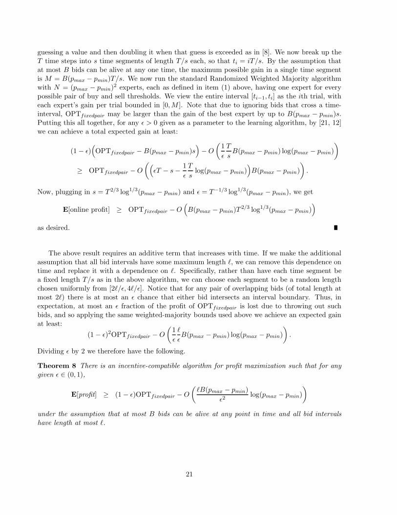
guessing a value and then doubling it when that guess is exceeded as in [8]. We now break up theT time steps into s time segments of length T/s each, so that ti = iT/s. By the assumption thatat most B bids can be alive at any one time, the maximum possible gain in a single time segmentis M = B(pmax − pmin)T/s. We now run the standard Randomized Weighted Majority algorithmwith N = (pmax − pmin)2 experts, each as defined in item (1) above, having one expert for everypossible pair of buy and sell thresholds. We view the entire interval [ti−1, ti] as the ith trial, witheach expert’s gain per trial bounded in [0,M ]. Note that due to ignoring bids that cross a time-interval, OPTfixedpair may be larger than the gain of the best expert by up to B(pmax − pmin)s.Putting this all together, for any ε > 0 given as a parameter to the learning algorithm, by [21, 12]we can achieve a total expected gain at least:

(1− ε)(

OPTfixedpair −B(pmax − pmin)s)

−O

(

1

ε

T

sB(pmax − pmin) log(pmax − pmin)

)

≥ OPTfixedpair −O

(

(

εT − s−1

ε

T

slog(pmax − pmin)

)

B(pmax − pmin)

)

.

Now, plugging in s = T 2/3 log1/3(pmax − pmin) and ε = T−1/3 log1/3(pmax − pmin), we get

E[online profit] ≥ OPTfixedpair −O(

B(pmax − pmin)T 2/3 log1/3(pmax − pmin))

as desired.

The above result requires an additive term that increases with time. If we make the additionalassumption that all bid intervals have some maximum length `, we can remove this dependence ontime and replace it with a dependence on `. Specifically, rather than have each time segment bea fixed length T/s as in the above algorithm, we can choose each segment to be a random lengthchosen uniformly from [2`/ε, 4`/ε]. Notice that for any pair of overlapping bids (of total length atmost 2`) there is at most an ε chance that either bid intersects an interval boundary. Thus, inexpectation, at most an ε fraction of the profit of OPTfixedpair is lost due to throwing out suchbids, and so applying the same weighted-majority bounds used above we achieve an expected gainat least:

(1− ε)2OPTfixedpair −O

(

1

ε

`

εB(pmax − pmin) log(pmax − pmin)

)

.

Dividing ε by 2 we therefore have the following.

Theorem 8 There is an incentive-compatible algorithm for profit maximization such that for anygiven ε ∈ (0, 1),

E[profit] ≥ (1− ε)OPTfixedpair −O

(

`B(pmax − pmin)

ε2log(pmax − pmin)

)

under the assumption that at most B bids can be alive at any point in time and all bid intervalshave length at most `.

21

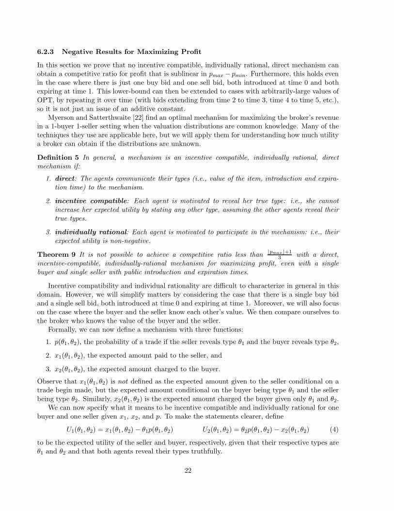
6.2.3 Negative Results for Maximizing Profit

In this section we prove that no incentive compatible, individually rational, direct mechanism canobtain a competitive ratio for profit that is sublinear in pmax − pmin. Furthermore, this holds evenin the case where there is just one buy bid and one sell bid, both introduced at time 0 and bothexpiring at time 1. This lower-bound can then be extended to cases with arbitrarily-large values ofOPT, by repeating it over time (with bids extending from time 2 to time 3, time 4 to time 5, etc.),so it is not just an issue of an additive constant.

Myerson and Satterthwaite [22] find an optimal mechanism for maximizing the broker’s revenuein a 1-buyer 1-seller setting when the valuation distributions are common knowledge. Many of thetechniques they use are applicable here, but we will apply them for understanding how much utilitya broker can obtain if the distributions are unknown.

Definition 5 In general, a mechanism is an incentive compatible, individually rational, directmechanism if:

1. direct: The agents communicate their types (i.e., value of the item, introduction and expira-tion time) to the mechanism.

2. incentive compatible: Each agent is motivated to reveal her true type: i.e., she cannotincrease her expected utility by stating any other type, assuming the other agents reveal theirtrue types.

3. individually rational: Each agent is motivated to participate in the mechanism: i.e., theirexpected utility is non-negative.

Theorem 9 It is not possible to achieve a competitive ratio less than bpmaxc+13 with a direct,

incentive-compatible, individually-rational mechanism for maximizing profit, even with a singlebuyer and single seller with public introduction and expiration times.

Incentive compatibility and individual rationality are difficult to characterize in general in thisdomain. However, we will simplify matters by considering the case that there is a single buy bidand a single sell bid, both introduced at time 0 and expiring at time 1. Moreover, we will also focuson the case where the buyer and the seller know each other’s value. We then compare ourselves tothe broker who knows the value of the buyer and the seller.

Formally, we can now define a mechanism with three functions:

1. p(θ1, θ2), the probability of a trade if the seller reveals type θ1 and the buyer reveals type θ2,

2. x1(θ1, θ2), the expected amount paid to the seller, and

3. x2(θ1, θ2), the expected amount charged to the buyer.

Observe that x1(θ1, θ2) is not defined as the expected amount given to the seller conditional on atrade begin made, but the expected amount conditional on the buyer being type θ1 and the sellerbeing type θ2. Similarly, x2(θ1, θ2) is the expected amount charged the buyer given only θ1 and θ2.

We can now specify what it means to be incentive compatible and individually rational for onebuyer and one seller given x1, x2, and p. To make the statements clearer, define

U1(θ1, θ2) = x1(θ1, θ2)− θ1p(θ1, θ2) U2(θ1, θ2) = θ2p(θ1, θ2)− x2(θ1, θ2) (4)

to be the expected utility of the seller and buyer, respectively, given that their respective types areθ1 and θ2 and that both agents reveal their types truthfully.

22

1. The mechanism is incentive compatible if for all θ1, θ2, θ′1, θ

′2 ∈ [pmin, pmax]:

U1(θ1, θ2) ≥ x1(θ′1, θ2)− θ1p(θ′1, θ2) U2(θ1, θ2) ≥ θ2p(θ1, θ

′2)− x2(θ1, θ

′2) (5)

2. The mechanism is individually rational if for all θ1, θ2 ∈ [pmin, pmax]:

U1(θ1, θ2) ≥ 0 U2(θ1, θ2) ≥ 0 (6)

Finally, the expected profit of the broker is:

U0(θ1, θ2) = x2(θ1, θ2)− x1(θ1, θ2) = (θ2 − θ1)p(θ1, θ2)− U2(θ1, θ2)− U1(θ1, θ2) (7)

Theorem 10 If an online direct mechanism is incentive compatible, then for all θ1,θ2, p(θ1, θ2) isweakly decreasing in θ1 and weakly increasing in θ2, and:

U1(θ1, θ2) = U1(pmax, θ2) +

∫ pmax

θ1

p(s1, θ2)ds1 U2(θ1, θ2) = U2(θ1, 0) +

∫ θ2

0p(θ1, s2)ds2

The proof of Theorem 10 follows quite closely the beginning of Theorem 1 of Hagerty andRogerson [16] where they prove a similar result for budget-balanced auctions. As is shown in [22],extending such a result beyond the budget-balanced case is not hard. See Chapter 3 of Zinkevich[29] for a full version of the proof.

Define n = bpmaxc. Consider the n pairs of types for the seller and the buyer, (0, 1), (1, 2), . . . , (n−1, n). Observe that the optimal broker achieves a value of 1 in any of these scenarios. If p is theprobability of trade for the online algorithm, define

p1 = mini∈1...n

p(i− 1, i).

Notice that by equation (7), the competitive ratio of the online algorithm can be no more than 1p1

if it satisfies individual rationality. We now show a recursive bound that gives an upper bound onp1.

Lemma 2 Define p∆ such that:p∆ = min

i∈∆...np(i−∆, i).

If the mechanism has a finite competitive ratio then for all ∆ > 1, p∆ ≥∆+1

3 p1.

Proof: Define

p∗∆ =

p1 if ∆ = 1∆+1

3 p1 otherwise.

We now argue by induction. Assume that the theorem holds for all ∆′ < ∆. Now, combiningEquations (6), (7), and Theorem 10 we have that for any integer a ∈ ∆, n:

U0(a−∆, a) ≤ tp(a−∆, a)−

∫ pmax

a−∆p(s1, a)ds1 −

∫ a

0p(a−∆, s2)ds2

23

Since p is nonnegative, decreasing in its first argument, and increasing in its second argument, thiscan be bounded above by:

U0(a−∆, a) ≤ ∆p(a−∆,∆)−

∫ a−1

a−∆p(s1, a)ds1 −

∫ a

1+a−∆p(a−∆, s2)ds2

≤ ∆p(a−∆,∆)−

a−1∑

s1=1+a−∆

p(s1, a)−

a−1∑

s2=1+a−∆

p(a−∆, s2).

By the definition of p∆′ , this can be bounded above by:

U0(a−∆, a) ≤ ∆p(a−∆,∆)− 2

∆−1∑

∆′=1

p∆′ .

In order to obtain a finite competitive ratio, the expected utility of the broker must be nonnegativeregardless of the types of the agents. Thus U0(a−∆, a) ≥ 0, and:

p(a−∆,∆) ≥2

∆

∆−1∑

∆′=1

p∆′

By the inductive hypothesis

p(a−∆,∆) ≥2

∆

∆−1∑

∆′=1

p∗∆′ .

Since a is any integer in ∆, . . . , n:

p∆ ≥2

∆

∆−1∑

∆′=1

p∗∆′ =2

∆

(

1 +∆−1∑

∆′=2

∆′ + 1

3

)

p1 =2

∆

(

∆(∆ + 1)

6

)

p1 =∆ + 1

3p1.

Proof (of Theorem 9): ¿From the above lemma, p(0, n) ≥ n+13 p1. This implies that p1 ≤

3n+1 ,

and the competitive ratio is no less than bpmaxc+13 .

In a dominant strategy mechanism, the bidders can have strategies that are more complex.However, the strategy of a bidder must be optimal regardless of the other agents’ bids, and everybidder must be motivated to participate.8 In this case, using a similar technique, we can get asimilar bound.

Theorem 11 No dominant strategy mechanism can achieve a competitive ratio for profit lowerthan pmax−pmin

3 .

8Therefore, a direct mechanism that is incentive compatible and individually rational for any pair of valuations isa dominant strategy mechanism.

24

Objective Upper bound Lower bound

Profit (non-IC) ln(pmax − pmin) + 1 ln(pmax − pmin) + 1

Profit (non-IC) (1 + ε) wrt fixed thresholdwith assumptions

Profit (IC) pmax − pmin Ω(pmax − pmin)

Profit (IC) (1 + ε) wrt fixed priceswith assumptions

# trades (non-IC) 2 (no subsidy) 4/3 (no subsidy)1 (with subsidy)

Buy/sell volume (non-IC) 2(ln(pmax/pmin) + 1) (no subsidy) ln(pmax/pmin) + 1ln(pmax/pmin) + 1 (with subsidy)

Social welfare (non-IC) r = ln pmax

(r−1)pminr = ln pmax

(r−1)pmin

Social welfare (IC) 2max(2, ln(pmax/pmin))

Table 1: Main results of this paper.

7 Conclusions and Open Questions

In this paper, we have derived bounds on competitive ratios for a number of basic online marketclearing problems. These include the objectives of maximizing profit, maximizing liquidity accord-ing to several natural measures, and maximizing social welfare. Using the abstraction of onlineincomplete interval graphs, we obtain algorithms that achieve best-possible competitive ratios formost of these problems, and for the rest we are within a factor of two of the best that is achievableonline. For the objective of maximizing number of trades, we demonstrate that by allowing theonline algorithm to subsidize matches with profits from previous trades, we can perform as well asthe optimal offline algorithm without subsidy. Thus the ability to subsidize trades is at least aspowerful as knowing the future, in this context.

It is a somewhat unfortunate fact about competitive analysis that no algorithm can guaranteebetter than a logarithmic ratio for maximizing profit. This lower bound occurs because we arecomparing the performance of our online algorithm to the best performance of any arbitrary algo-rithm in hindsight. However, if we restrict our comparison class to a fixed, finite set of algorithms(such as the class of all fixed-threshold algorithms), and if we assume the data is not too “bursty”,then we can use online learning results to achieve a 1 + ε ratio, as we demonstrate in Section 5.1.

We also consider the issue of incentive compatibility, and show that our Greedy algorithm isincentive-compatible for the goal of maximizing social welfare. Thus, losing only a factor of 2 incompetitive ratio we can achieve this desirable property. In fact, we show the Greedy algorithm isquite robust in that it maintains its competitive ratio even if bidders are allowed to modify theirbids over time, making the task even harder on the online algorithm. For profit maximization,we show that no direct algorithm can achieve a sublinear competitive ratio, though we present analgorithm that has competitive ratio approaching 1 with respect to the best fixed pair of buy/sellprices when bids are not too bursty. We summarize our main results in Table 1.

25

Open problems

There are a number of open problems with respect to incentive-compatibility. For example in termsof competing with respect to the best fixed pair of buy and sell prices for profit maximization, ourresults require that bids not be too “bursty” (at most B alive at any one time). On the otherhand, [9] provide algorithms for the offline problem where all bids are concurrent. Perhaps somecombination can handle the general case.

There is also a gap between our best upper bound (2) and our best lower bound (3/2) foralgorithms for the incomplete interval graph vertex-selection problem when expiration times areunknown. Algorithm 2 achieves an optimal matching but it needs to know the expiration times inadvance. Related to this question, we do not know whether the Greedy algorithm can be improvedupon for the setting of Section 5.2 in which a bidder may submit a bid whose value varies withtime.

There has also been recent interest in offline clearing algorithms for combinatorial exchangeswhere a bid can concern multiple distinguishable items (possibly multiple units of each) [23, 25, 26].A bid could state, for example, “I want to buy 20 IBM, buy 50 DELL, sell 700 HP, and getpaid $500”. As we transformed the online clearing problem to an online matching problem in anincomplete interval graph, the online problem of maximizing profit or liquidity in a combinatorialexchange can be transformed to the problem of finding a matching on an incomplete intervalhypergraph online. While we can show with a simple example that a maximum matching cannotbe achieved online in the hypergraph problem, it might be possible to achieve a matching with anexpected size no less than half of the maximum one.

One direction of future research is to extend these results to settings where there is a marketmaker who can carry inventory of the commodity (sell short and long) rather than simply decidingwhich bids to match.

Acknowledgements

The authors would like to thank Ke Yang for a number of helpful suggestions. This materialis based upon work supported under NSF grants CCR-9732705, CCR-0085982, CAREER AwardIRI-9703122, IIS-9800994, ITR IIS-0081246, ITR IIS-0121678, and an NSF Graduate ResearchFellowship. Sandholm was also funded by a Sloan Fellowship. Any opinion, findings, conclusionsor recommendations expressed in this publication are those of the authors and do not necessarilyreflect the views of the National Science Foundation or the Sloan Foundation.

References

[1] B. Awerbuch, Y. Bartal, A. Fiat, and A. Rosen. Competitive non-preemptive call control. InProceedings of the 5th Symposium on Discrete Algorithms (SODA), pages 312–320, 1994.

[2] A. Bagchi, A. Chaudhary, R. Garg, M. Goodrich, and V. Kumar. Seller-focused algorithmsfor online auctioning. In Proceedings of WADS 2001, pages 135–147, 2001.

[3] Z. Bar-Yossef, K. Hildrum, and F. Wu. Incentive-compatible online auctions for digital goods.In Proceedings of the 13th Symposium on Discrete Algorithms (SODA), 2002.

[4] C. Berge. Two theorems in graph theory. In Proceedings of the National Academy of Sciences,volume 43, pages 842–844, 1957.

26

[5] A. Blum and C. Burch. On-line learning and the metrical task system problem. MachineLearning, 39(1):35–58, April 2000.

[6] A. Blum, V. Kumar, A. Rudra, and F. Wu. Online Learning in Online Auctions. In Proc. 14thSymposium on Discrete Algorithms. ACM/SIAM, 2003.

[7] A. Borodin and R. El-Yaniv. Online Computation and Competitive Analysis. CambridgeUniversity Press, 1998.

[8] N. Cesa-Bianchi, Y. Freund, D. Helmbold, D. Haussler, R. Schapire, and M. Warmuth. Howto use expert advice. Journal of the ACM, 44(3):427–485, 1997.

[9] K. Deshmukh, A. Goldberg, J. Hartline, and A. Karlin. Truthful and competitive doubleauctions. In ESA ’02: Proceedings of the 10th Annual European Symposium on Algorithms,pages 361–373. Springer-Verlag, 2002.

[10] I. Domowitz. Automating the continuous double auction in practice: Automated trade exe-cution systems in financial markets. In Daniel Friedman and John Rust, editors, The DoubleAuction Market, volume 14 of Santa Fe Institute Studies in the Sciences of Complexity, pages27–60. Addison-Wesley, 1993.

[11] R. El-Yaniv, A. Fiat, R. Karp, and G. Turpin. Competitive analysis of financial games. InProc. 33rd Symp. Foundations of Computer Science, pages 327–333, 1992.

[12] Y. Freund and R. Schapire. Game theory, on-line prediction and boosting. In Proc. 9th Conf.on Computational Learning Theory, pages 325–332, 1996.

[13] A. Goldberg, J. Hartline, and A. Wright. Competitive auctions and multiple digital goods.Technical report, InterTrust 00-01, 2000.

[14] A. Goldberg, J. Hartline, and A. Wright. Competitive auctions and digital goods. In AnnualACM-SIAM Symposium on Discrete Algorithms (SODA), Washington, DC, 2001.

[15] S. Goldman, J. Parwatikar, and S. Suri. On-line scheduling with hard deadlines. Journal ofAlgorithms, 34:370–389, 2000.

[16] K. Hagerty and W. Rogerson. Robust trading mechanisms. Journal of Economic Theory,42:94–107, 1987.

[17] R. Karp, U. Vazirani, and V. Vazirani. An optimal algorithm for on-line bipartite matching.In Proc. 22nd Symp. Theory of Computing, pages 352–358, Baltimore, Maryland, 1990.

[18] D. Kozen. The Design and Analysis of Algorithms. Springer-Verlag, New York, 1991.

[19] R. Lavi and N. Nisan. Competitive analysis of incentive compatible on-line auctions. In Pro-ceedings of the ACM Conference on Electronic Commerce (ACM-EC), pages 233–241, Min-neapolis, MN, 2000.

[20] R. Lipton and A. Tomkins. Online interval scheduling. In Proc. 5th Symp. on Discrete Algo-rithms, pages 302–311, 1994.

[21] N. Littlestone and M. Warmuth. The weighted majority algorithm. Information and Compu-tation, 108:212–261, 1994.

27

[22] R. Myerson and M. Satterthwaite. Efficient mechanisms for bilateral trading. Journal ofEconomic Theory, 28:265–281, 1983.

[23] T. Sandholm. eMediator: A next generation electronic commerce server. ComputationalIntelligence, 18(4):656–676, 2002. Special issue on Agent Technology for Electronic Commerce.

[24] T. Sandholm and S. Suri. Optimal clearing of supply/demand curves. In 13th Annual Interna-tional Symposium on Algorithms and Computation (ISAAC), Vancouver, Canada, November2002. Also appeared in the proceedings of the AAAI-02 workshop on Agent-Based Technolo-gies for B2B Electronic Commerce (AAAI Technical Report WS-02-01), pp. 15–22, Edmonton,Canada.

[25] T. Sandholm and S. Suri. BOB: Improved winner determination in combinatorial auctionsand generalizations. Artificial Intelligence, 145:33–58, 2003.

[26] T. Sandholm, S. Suri, A. Gilpin, and D. Levine. Winner determination in combinatorialauction generalizations. In International Conference on Autonomous Agents and Multi-AgentSystems (AAMAS), pages 69–76, Bologna, Italy, July 2002.

[27] P. Wurman, M. Wellman, and W. Walsh. The Michigan Internet AuctionBot: A configurableauction server for human and software agents. In Proceedings of the Second InternationalConference on Autonomous Agents (AGENTS), pages 301–308, Minneapolis/St. Paul, MN,May 1998.

[28] P. Wurman, W. Walsh, and M. Wellman. Flexible double auctions for electronic commerce:Theory and implementation. Decision Support Systems, 24(1):17–27, 1998.

[29] M. Zinkevich. Theoretical Guarantees for Algorithms in Multiagent Settings. Ph.D. Thesis,Carnegie Mellon University, August 2004.

Appendices

A Lemmas on Matchings

In this section, we prove some lemmas required for the proof of the main theorem in Appendix B.We will use some standard facts and definitions from graph theory; for a review, see [18]. Paths willbe represented as sets of edges, although sometimes it will be easier to write them as a sequence ofvertices. V (P ) is the set of vertices of a path P . We will also use some well known lemmas:

Lemma 3 Given W ⊂ V , a perfect matching M on W , and v, v′ ∈ V −W , if there exists someaugmenting path P with respect to M from v to v′, then M⊕P is a perfect matching on W ∪v, v′.

Lemma 4 The symmetric difference of two matchings M and M ′ consists of alternating paths andalternating cycles with respect to M .

Lemma 5 A vertex v ∈ V is the endpoint of an alternating path in the symmetric difference oftwo matchings M and M ′ if and only if it is in V (M)⊕ V (M ′).

28

Proof: Suppose a vertex is in V (M) ⊕ V (M ′). Then it has an incident edge in either M or M ′,but not both. Hence, it can only have one incident edge in M ⊕M ′, making it an endpoint of analternating path.

Suppose a vertex is at the endpoint of a path in M ⊕M ′. Then it has one edge in M ⊕M ′.Observe that if it has an odd number of edges incident to it in M ⊕M ′, the number of edges in Mto it plus the number of edges in M ′ to it is also odd. But since the latter is bounded by zero andtwo, it is one. Therefore, the vertex cannot be in both V (M) and V (M ′).

Augmenting paths capture some of the local properties of matchings. But they do not capturehow to remove elements from a matching, or how to replace an element. Since these are importantconcepts in the online setting, we introduce some other types of paths. These paths have propertiesvery similar to those of augmenting paths.

Definition 6 An abridging path with respect to a matching M is an alternating path whose firstand last edges are in M . A replacement path with respect to M is an alternating path whose firstedge is in M , and whose last endpoint is not in V (M).

Lemma 6 Given v, v′ ∈ W , and a perfect matching M on W , if there exists some abridging pathP with respect to M from v to v′, then M ⊕ P is a perfect matching on W − v, v′.

The proof is similar to the proof of Lemma 3.

Lemma 7 Given v ∈ W and v′ ∈ V − W , and a perfect matching M on W , if there existssome replacement path P with respect to M from v to v′, then M ⊕ P is a perfect matching onW ∪ v′ − v.

The proof is similar to the proof of Lemma 3.

Lemma 8 Suppose W and W ′ are subsets of V , and there exists a perfect matching on W and aperfect matching on W ′, then there exists a partition of W ⊕W ′ into sets of size two:

a1, b1, a2, b2, . . . , ak, bk

such that for all 1 ≤ i ≤ k, there exists a perfect matching on W ⊕ ai, bi.

Proof: Define M to be a perfect matching on W and M ′ to be a perfect matching on W ′. ThenM ⊕M ′ consists of a set of alternating paths and cycles. Here, we are only concerned with thepaths. Since these paths only begin and end at points in W ⊕W ′, we can partition W ⊕W ′ whereeach set is the set of endpoints of a path in M ⊕M ′. Consider a set in this partition a, b, whereP is the path between the two elements of the set. There are three possibilities:

1. Both vertices are in W ′−W . Then P is an augmenting path, and M⊕P is a perfect matchingon W ∪ a, b = W ⊕ a, b.

2. One vertex is in W −W ′ and one vertex in W ′−W . In this case, the path P is a replacementpath. Without loss of generality, assume a ∈W −W ′. Then M ⊕P is a perfect matching onW ∪ b − a = W ⊕ a, b.

29

3. Both vertices are in W−W ′. The first and last edges are not in M ′, because a and b are not inW ′. Also, the first and last edges are in M⊕M ′ ⊆M ∪M ′. Therefore, the first and last edgesare in M , and P is an abridging path. M⊕P is a perfect matching on W−a, b = W⊕a, b.

Corollary 2 If W ⊆ V has a perfect matching, but it is not one of the largest sets that has aperfect matching, then there exists v, v′ ∈ V −W such that W ∪ v, v′ has a perfect matching.

B Proof of Theorem 2 (Main Theorem)

Assume W is the set of selected vertices, then we define H1,H2, and H3 as follows:

H1: For any expired, unmatched vertex w, there does not exist any untaken vertex w′ such thatthere is a perfect matching on W ∪ w,w′.

H2: For any matched vertex w, there does not exist an untaken vertex w′ such that there is aperfect matching on W ∪ w′ − w and tf (w) > tf (w′).

H3: For any two unexpired vertices w,w′ ∈W , there exists no perfect matching on W − w,w′.

Let H denote the conjunction of the three invariants H1, H2, and H3. We will prove that if theseinvariants of the algorithm hold before an event occurs, they will hold after the event. The possibleevents that can occur are a vertex being introduced, expiring without being matched, or expiringand being added.

Lemma 9 If H holds before a vertex w′ is introduced, H holds after the event.

Proof: We prove this for all three parts of H.

H1: Consider w to be an expired, unmatched vertex. Here we need to prove that there existsno perfect matching on W ∪ w,w′. We will prove this by contradiction. Suppose thatM is a perfect matching on W ∪ w,w′. Define v such that (w′, v) ∈ M . Let us defineM ′ = M −(w′, v). Then, M ′ is a perfect matching on W −v+ w. Since w has expiredand v has not expired, tf (w) < tf (v). This contradicts the inductive hypothesis H2.

H2: Suppose that w ∈W and tf (w) > tf (w′). We need to prove that there does not exist a perfectmatching for W ∪ w′ − w by contradiction, assuming there exists a perfect matching M .

Define v such that (w′, v) ∈M . Observe that tf (v) > ti(w′), so v has not expired. Neither has

w, since tf (w) > tf (w′) > ti(w′). However, M − (w′, v) is a perfect matching on W − w, v.

This is a contradiction of H3.

H3: This cannot have any effect.

Lemma 10 If H holds before a vertex w expires without being matched, H holds after the event.

Proof: We prove this for all three parts of H.

30

H1: Suppose w′ is an untaken vertex. We need to prove that there does not exist a perfectmatching on W ∪ w,w′.

(a) Assume w′ expired. By H1, there there did not exist a perfect matching on W ∪w,w′.

(b) If there existed an unexpired, unmatched vertex w′ such that W ∪w,w′ had a perfectmatching, then w would have been matched.

H2,H3: This cannot have any effect.

Lemma 11 If H holds before a vertex v expires and is added with v′, H holds after the event.

Proof: We prove this for all three parts of H.

H1: Suppose w is an expired, unmatched vertex, and w′ is an untaken vertex. We need to provethat there does not exist a perfect matching on W ∪ v, v′, w,w′. We can prove this bycontradiction.

Observe that there exists a perfect matching on W . If there existed a perfect matching onW ∪ v, v′, w,w′, then by Lemma 8 one of the following conditions holds:

(a) There exists a perfect matching on W ∪ v′, w. This would contradict H1.

(b) There exists a perfect matching on W ∪ v,w. This would contradict H1.

(c) There exists a perfect matching on W ∪ w,w′. This would contradict H1.

H2: Consider an arbitrary vertex w in W ∪ v, v′, and an arbitrary untaken vertex w′. Assumethat W ∪ v, v′, w′ − w is a perfect matching. We must prove that tf (w′) ≥ tf (w).

(a) w = v. Then W ∪ v, v′, w′ − w = W ∪ v′, w′. So by H1, w′ has not expired. Thentf (w′) ≥ tf (w), because w is just expiring.

(b) w = v′. Then W ∪ v, v′, w′ − w = W ∪ v,w′. So by H1, w′ has not expired. Thusif tf (w) > tf (w′), then w′ would have been added instead of w.

(c) w ∈W . Then by Lemma 8 applied to W and W ∪v, v′, w′−w, one of the followingconditions holds:

i. W ∪ v − w and W ∪ v′, w′ have perfect matchings. Then by H1, w′ has notexpired, and tf (w) < tf (v), so w has expired.

ii. W ∪ v′ − w and W ∪ v,w′ have perfect matchings. Then by H1, w′ has notexpired, so tf (w′) ≥ tf (v′). Also, tf (w) ≤ tf (v′).

iii. W ∪ w′ − w has a perfect matching. Then by H2, tf (w′) ≥ tf (w).

H3: A vertex v expires and is added with v′. Suppose that w,w′ ∈ W ∪ v, v′. Assume thatW ∪ v, v′ − w,w′ has a perfect matching. We must prove that w or w′ has expired.Consider three cases:

(a) w = v. Then w has expired.

(b) w = v′. Then W ∪ v, v′ − w,w′ = W ∪ v − w′. Thus by H2, tf (v) ≥ tf (w′), sow′ has already expired(a contradiction).

31

(c) w ∈W . Then by Lemma 8 applied to W and W ∪v, v′−w,w′, one of the followingconditions holds:

i. W ∪ v − w has a perfect matching. By H2, tf (v) ≥ tf (w), so w has expired.ii. W ∪ v − w′ has a perfect matching. By H1, tf (v) ≥ tf (w′), so w′ has expired.iii. W − w,w′ has a perfect matching. By H3, either w or w′ has expired.

Proof (of Theorem 2): We will prove by induction that H holds at the termination of the al-gorithm. First, observe that H1, H2, and H3 are all properties of introduced vertices, so when thereare no vertices introduced, they cannot be violated. This is the base case. Inductively, by Lem-mas 9, 10, 11, if these properties hold before an event, they hold afterward as well. Thus, H holdsat the termination of the algorithm. Specifically, H1 implies that there exists no v, v′ ⊆ V −Wsuch that W ∪ v, v′ has a perfect matching. By Corollary 2, W is one of the largest sets with aperfect matching.

C Proof of Theorem 5 (Performing nearly as well as the best

threshold in hindsight)

The setting is we have N algorithms (“experts”) and we can switch from one to another at cost≤ D. At each time step (introduction of a bid) the algorithms experience gains between 0 andgmax. (We use gmax instead of pmax because we will be using “p” for probabilities). At any point intime, our overall “master” algorithm will be a probability distribution over the N base algorithms.Specifically, we use the standard multiplicative-weights algorithm [21, 12] as follows:

• We begin with each base algorithm having a weight wi = 1. Let W =∑

i wi. Our probabilitydistribution over base algorithms will be pi = wi/W .

• After each event, we update weights according to the rule:

wi ← wi(1 + ε)gi/gmax ,

where gi is the gain of the ith algorithm, and ε is defined below. We then update ourprobability distribution pi accordingly. Note: if ~p is the old distribution and ~p′ is the newdistribution, we can do this such that the expected movement cost is at most D

2 L1(~p, ~p′) whereL1(~p, ~p′) is the L1 distance between the two distributions.

Theorem 12 If we use ε = εgmax

2D , and under the assumption that D ≥ gmax, the above algorithmproduces an expected gain at least

OPT(1− ε)−2D

εln N,

where OPT is the gain of the best of the N base algorithms in hindsight.

32

Proof: Suppose the algorithm currently has weights w1, . . . , wn, observes a gain vector g1, . . . , gn

and then updates the weights to w′1, . . . , w

′n, where w′

i = wi(1 + ε)gi/gmax . Let W =∑

i wi and letW ′ =

∑

i w′i. Let pi = wi/W and let p′i = w′

i/W′.

The expected gain of the online algorithm from this event is∑

i pigi, which we will call Et ifthis is event t. The expected cost due to moving from probability distribution ~p to distribution ~p′

is at most

D∑

i:p′i>pi

(p′i − pi) ≤D

W

∑

i:p′i>pi

(w′i − wi) ≤

D

W(W ′ −W ) = D

(

W ′

W− 1

)

,

where the first inequality above uses the fact that W ′ ≥W , and the second inequality uses the factthat w′

i ≥ wi for all i, not just the ones such that p′i > pi.The next step in the analysis is to upper bound W ′ as a function of W . To do this, we use the

fact that for x ≤ 1, (1 + α)x ≤ 1 + xα. So,

W ′ ≤∑

i

wi

(

1 +εgi

gmax

)

= W∑

i

pi

(

1 +εgi

gmax

)

= W

(

1 +ε

gmaxEt

)

.

This upper bound on W ′ is useful in two ways. First, we can now analyze the expected movementcost: D(W ′/W − 1) ≤ D( ε

gmaxEt). So, our total expected gain for event t is at least Et(1−

Dεgmax

).Second, we can use this to give an upper bound on the total weight Wfinal at the end of the

process:

Wfinal ≤ N∏

t

(

1 +ε

gmaxEt

)

.

This upper bound can be compared to a lower bound

Wfinal ≥ (1 + ε)OPT/gmax

which is simply the final weight of the best of the N algorithms. Taking logs on the upper andlower bounds to Wfinal and using the fact that ln(1 + x) ∈ [x− x2/2, x] for x ∈ [0, 1], we have:

(OPT/gmax)(ε− ε2/2) ≤ (OPT/gmax) ln(1 + ε) ≤ ln N +∑

t

ln(1 +ε

gmaxEt) ≤ ln N +

ε

gmax

∑

t

Et.

So,∑

t

Et ≥ OPT(1− ε/2)−gmax

εln N.

Finally, using the fact that the total expected gain Galg (with movement costs included) is at least(1− Dε

gmax)∑

t Et, and using our definition ε = εgmax/(2D), we have:

Galg ≥ OPT(1− ε/2)(1 − ε/2) − (1− ε/2)2D

εln N ≥ OPT(1− ε)−

2D

εln N.

33