Embed Size (px)
Citation preview

CCOONNFFEERREENNCCEE OONN IINNTTEERRNNAATTIIOONNAALL MMAACCRROO--FFIINNAANNCCEE
AAPPRRIILL 2244--2255,, 22000088
The Decomposition of the U.S. External Returns
Differential
Stephanie E. Curcuru, Tomas Dvorak, and Francis E. Warnock
Presented by Frank Warnock


The Decomposition of the U.S. External Returns Differential*
Stephanie E. Curcuru
Board of Governors of the Federal Reserve System
Tomas Dvorak
Union College
Francis E. Warnock
Darden Graduate School of Business, University of Virginia
Institute for International Integration Studies, Trinity College Dublin
Globalization and Monetary Policy Institute, Federal Reserve Bank of Dallas
National Bureau of Economic Research
April 21, 2008
Prepared for the April 24-25 2008 IMF Conference on International Macro-Finance
Abstract
We examine the returns differential between U.S. portfolio claims and liabilities and identify a
quantitatively and statistically important role for the timing of shifts between asset classes.
Specifically, we find that the poor timing of foreign investors when reallocating between U.S.
bonds and U.S. equities contributes positively to the U.S. external returns differential. While part
of this poor timing is due to the lack of portfolio rebalancing, most of it is due to deliberate
trading. The poor timing of trades across asset classes is not driven by mechanical reserve
accumulation, is particularly pronounced, and appears to be persistent across subsamples.
* This paper was previously circulated as ―The Stability of Large External Imbalances: The Role of
Returns Differentials‖. The views in this paper are solely the responsibility of the author(s) and should not
be interpreted as reflecting the views of the Board of Governors of the Federal Reserve System, the Federal
Reserve Bank of Dallas, or of any other person associated with the Federal Reserve System. We thank for
helpful comments Carol Bertaut, Ricardo Caballero, Charles Engel, Kristen Forbes, Gian-Maria Milesi-
Ferretti, Cedric Tille, Charles Thomas, Ralph Tryon, Eric van Wincoop, Jon Wongswan, and seminar
participants at the Dallas Fed and the European University Institute. Warnock thanks the Darden School
Foundation for its generous support.

1. Introduction
The year 2007 proved to be a volatile one for financial markets. It was also a year
with individual months of both record net foreign purchases and record net foreign sales
of U.S. stocks. The record net foreign purchases occurred in May, only to be followed by
1.7 and 3.1 percent declines in the S&P500 in June and July. The record net foreign sales
occurred in August, only to be followed by a 3.7 percent rise in the S&P500 in
September. In October, foreigners again piled into U.S. stocks, recording the second
highest net purchases on record. The following month, the S&P500 lost 4.2 percent.
Thus, 2007 could not have been a happy year for foreign investors in U.S. equities. On
top of a nine percent dollar depreciation against major currencies, foreigners seem to
have timed their equity purchases and sales wrong—being net buyers when the market
was about to fall and net sellers when the market was poised to rise.
In this paper we investigate the impact of market timing—specifically,
reallocating across portfolio asset classes—on the performance of foreign investors in the
U.S. compared to that of U.S. investors abroad. Focusing on bond and equity portfolios,
we calculate the returns differential between what U.S. investors earn abroad and what
foreign investors earn in the U.S. We decompose the returns differential into three
components: the composition, return, and timing effects. The first two—the composition
and return effects—capture average characteristics of U.S. claims and liabilities. The
composition effect would be positive were U.S. claims on foreigners weighted toward
asset classes with higher average returns. The return effect would be positive were U.S.
investors to earn higher average returns within each asset class. The third effect, timing,
is driven by reallocations across different asset classes and captures investment skill as

2
given by the covariance between current weights and subsequent returns. A positive
covariance between current asset weights—themselves the outcome of a passive buy-and-
hold strategy or active trading—and subsequent asset returns would mean that portfolios
were correctly positioned to capture subsequent returns. If portfolio weights and
subsequent returns covary more positively in U.S. claims than in U.S. liabilities, U.S.
investors display more skill abroad than foreign investors in the U.S. and the timing
effect would be positive.
Understanding the sources of the returns differential is important for a number of
reasons. As pointed out by Lane and Milesi-Ferretti (2005), with large gross external
positions even a small returns differential has significant implications for the net
international investment position. From the perspective of the current global imbalances
it is important to understand the persistence of the returns differential. Identifying its
components may help us evaluate their likely persistence. Furthermore, documenting the
dynamics of gross asset class allocation is relevant to the growing literature on portfolio
dynamics in open economy macroeconomics (Engel and Matsumoto (2006), Devereux
and Saito (2006), Tille and Wincoop (2007)). Finally, evaluating timing ability of foreign
investors contributes to the literature on information asymmetries between foreign and
domestic investors (Dvorak (2005), Choe, Kho and Stulz (2005), Brennan et al. (2005)).
Our paper differs from existing work in two important ways. The first is
methodological. While the composition and return effects have been studied before
(Gourinchas and Rey (2007)), examining the role of timing in the returns differential is
new. Our decomposition, which is inspired by performance evaluation techniques from
the finance literature (Grinblatt and Titman (1993)), enables us to separate the effect of

3
average portfolio characteristics and market timing. This allows us to evaluate the
previously unexplored role of investment skill in the returns differential. The second way
our analysis differs from previous work is that we use information from actual bond and
equity portfolios. Previous work on the composition and return effects utilizes implied
returns from datasets that we show in Curcuru, Dvorak and Warnock (2008) are
internally inconsistent. In contrast, we utilize monthly data on the country and asset class
composition of U.S. portfolio claims and liabilities. By matching precise country and
asset class weights to corresponding total market returns (and by being careful with the
currency composition by asset class and country), we are able to obtain accurate
estimates of the returns differential and its underlying components. Using data on
bilateral positions also has the advantage of allowing us to distinguish differentials vis-à-
vis developed from those vis-à-vis developing countries.1
We find that the timing of reallocations across asset class is a quantitatively and
statistically important component of the overall returns differential. Specifically, we find
that foreign investors in the U.S. exhibit poor timing across asset classes, tending to have
a relatively high equity weight when U.S. equity prices have already peaked and a
relatively low equity weight when U.S. equity prices are poised to rise. U.S. portfolio
investors abroad also time their allocations between foreign stocks and foreign bonds
poorly but to a much lower degree than foreigners in the U.S. On net, the difference
between the timing of foreign investors in the U.S. and the timing of U.S. investors
1 It should be noted at the outset that by focusing on high quality data on bond and equity portfolios, we are
necessarily excluding foreign direct investment (FDI), another important component of cross-border
positions. There is a long-standing, positive returns differential for direct investment that most evidence
suggests owes to some combination of a maturity effect (much of the FDI in the United States is relatively
new, whereas U.S. direct investment abroad tends to have been placed a long time ago) and transfer pricing
(Mataloni 2000, Hung and Mascaro 2004 and Higgins et. al. 2007). However, Gros (2006), Bosworth et al.
(2007), and Heath (2007) argue that much of the differential on FDI owes to tax system effects, suggesting
that for FDI any differential may be more apparent than real.

4
abroad increases the overall annual returns differential by about one-half percentage
point. Thus, part of whatever returns differential exists owes to the poor timing of
foreign investors. Were foreigners to exhibit more skill within their U.S. portfolios, the
returns differential would be even smaller.
We also differentiate between two underlying components of the timing effect,
active trading and the more passive failure to reallocate after the portfolio‘s composition
is altered by valuation changes. The more active component—the trading effect, a
generally accepted metric of portfolio performance originated by Grinblatt and Titman
(1993)—summarizes the ability of countries to shift their investments into asset classes
that subsequently rise in value. We find that active trading plays an important role in the
poor timing of foreign investors. Thus, our evidence suggests that the pattern of ill-timed
purchases by foreign investors in the U.S. described in the introduction has occurred
systematically over our 12-year sample period. We find no such pattern in the active
trading of U.S. investors abroad.
We perform a number of robustness checks. First, we examine whether our results
are driven by the accumulation of U.S. bonds by foreign officials, in particular the
governments of emerging market countries. We find that this is not the case. The results
are actually much stronger for developed countries and carry through to private foreign
investors. The results are also robust to excluding countries with financial centers such as
the U.K. or Luxembourg. Finally, poor timing by foreign investors appears persistent
and statistically significant across different subsamples, suggesting that ill-timed
purchases represent a genuine difference in investment style rather than bad luck.

5
The paper proceeds as follows. In the next section we discuss the underlying data
on international portfolios and returns characteristics. In Section 3, after presenting the
returns differential, we decompose it into the composition, return, and timing effects and
then further decompose the timing effect into its active and passive components. Section
4 concludes.
2. Characteristics of U.S. Portfolio Claims and Liabilities
Our technique to form portfolio returns is as in Curcuru, Dvorak, and Warnock
(2008): Observe monthly portfolio weights and then calculate one-month returns using
indices that mimic (to the extent possible) the composition of those portfolios. In this
section we describe the underlying data as well as the characteristics of the resulting
bilateral bond and equity positions and within-asset-class returns.
2.1 Positions
We use the highest quality dataset available on the monthly portfolio debt and
equity investment positions of U.S. investors abroad and foreign investors in the United
States. See Bertaut and Tryon (2007) for a complete discussion of the technique used to
construct the monthly positions data, which will soon be part of a regular data release by
the Federal Reserve. Briefly, monthly bilateral investment positions are constructed using
two components of data reported by the Treasury International Capital Reporting System
(TIC): infrequent but highly accurate benchmark surveys of holdings (both foreign
holdings of U.S. securities and U.S. holdings of foreign securities) and net monthly
transactions (both net purchases of U.S. assets by foreigners and net purchases of foreign
assets by U.S. residents). Bertaut and Tryon (2007), building on a technique originated in
6
Thomas, Warnock, and Wongswan (2006), bring these data sources together to produce
high-quality estimates of monthly positions of foreigners in U.S. securities (―U.S.
liabilities‖) and U.S. positions in foreign securities (―U.S. claims‖). The data cover
portfolio investment in long-term securities, specifically debt instruments with greater-
than-one-year original maturity (―bonds‖) and equities.
Two features of our dataset should be noted. One, we include only those countries
for which we have at least fifty monthly observations on both equity and bond returns
between January 1994 and December 2005. This leaves us with nineteen developed
countries and nineteen emerging markets. These countries account for the majority of
U.S. portfolio investment abroad as well as the majority of foreign investment in the
United States.2 Two, the TIC data distinguish between private and official positions only
at the aggregate level, so our country-level analysis groups together official and private
investors. We recognize that foreign official purchases of U.S. assets may occur for
reasons other than mean-variance optimization. With the exception of Japan, private
positions dwarf official holdings in developed countries, but for emerging market
countries official positions are likely to be more important. In robustness checks we delve
further into this issue.
2.2 Returns
The monthly bilateral positions dataset provides time-varying portfolio weights.
To calculate one-month returns we must select the returns series that mimic (to the extent
possible) the composition of those portfolios. For U.S. securities, for returns on U.S.
2 In 2004, the countries in our sample account for 84 percent and 80 percent of U.S. equity and bond
investment abroad and 77 percent and 73 percent of all foreigners‘ equity and bond investment in the
United States. Of the international investment that we do not cover, Caribbean financial centers account for
more than half.

7
bonds we use the weighted average of Lehman Brothers U.S. Treasury, corporate and
agency bond indices, with the weights given by foreigners‘ positions in each respective
bond type. Foreign investors, especially those from emerging markets, tend to overweight
Treasury and Agency bonds relative to a market-capitalization benchmark such as the
Lehman Brothers Aggregate U.S. bond index, so it is important to use the actual weights
of foreign investors in the three types of bonds to produce an accurate measure of their
returns on U.S. bonds. For returns on U.S. equities we use the return on the gross MSCI
U.S. index. The index is market capitalization weighted and, with roughly 300 large and
liquid U.S. firms, is comparable to the S&P 500 (which prior to 2002 included some
foreign firms).
For foreign securities, for returns on foreign equities we use dollar returns on the
gross MSCI equity index for each country. MSCI indexes are appropriate because MSCI
firms represent almost 80 percent of U.S. investors‘ foreign equity investment (Ammer et
al. 2006). For foreign bonds, to a large extent U.S. investors tend to hold local currency
bonds in developed countries and dollar-denominated bonds in emerging markets (Burger
and Warnock, 2007). Thus, for developing countries we use J.P. Morgan‘s EMBI+
indices (which are comprised of dollar-denominated bonds). In those developed countries
where U.S. holdings of local currency bonds are predominant, we use the MSCI bond
index (which is an index of local-currency-denominated bonds). In those developed
countries where U.S. holdings of dollar-denominated bonds are significant we calculate
returns as the weighted average of the MSCI bond index and MSCI Eurodollar Credit
index (which is an index of dollar-denominated bonds), with the weights on the
Eurodollar index being the shares of dollar denominated bonds in U.S. holdings of

8
foreign bonds.3 When calculating returns on the aggregate foreign bond and foreign
equities portfolios, we weight each country according to U.S. bond (or equity) holdings in
that country. The average weight of each country in U.S. foreign equity and bond
portfolios and the average returns on each country‘s equities and bonds appear in Table I.
Our sample period covers the 144 months between January 1994 and December
2005. The starting point is determined by the availability of MSCI bond indices, which
begin in December 1993. The ending point is determined by the availability of U.S.
foreign asset positions, which are available through December 2005. For some countries,
equity or bond returns data begin after January 1994. We add these countries to the U.S.
asset and liability portfolios when the data for both equity and bond returns become
available (see the last column in Table I). Countries added after January 1994 tend to
have very low weights in both U.S. claims and liabilities portfolios, so our results are
nearly identical if we restrict our study to countries with returns data for the entire sample
period.
2.3 Descriptive statistics
Table II shows the descriptive statistics for aggregate equity weights in U.S.
portfolio claims and liabilities and aggregate returns on U.S. and foreign bonds and
equities. It is evident from Panels A and B that U.S. claims (that is, U.S. investors‘
foreign portfolios) are weighted heavily toward equities, while U.S. liabilities
(foreigners‘ portfolios in the U.S.) are weighted toward bonds. This resembles the
―venture capitalist‖ capital structure of the U.S. external balance sheet as pointed out by
Gourinchas and Rey (2007). Specifically, the mean equity-to-bond ratio in U.S. claims is
3 The developed countries where U.S. holdings of dollar denominated bonds are significant include
Australia, Belgium, Canada, Finland, France, Germany, Ireland, Netherlands, Sweden and the United
Kingdom.

9
71:29 across all countries, with equities having a higher weight in U.S. investors‘
developed country portfolios (72:28 equity-to-bond ratio) than in the emerging market
portfolios (60:40). By contrast, the mean equity-to-bond ratio in U.S. liabilities is 42:58,
roughly that (46:54) for developed countries‘ positions, but much lower for emerging
markets‘ portfolios (9:91).
Equity and bond returns are shown in Panels C and D, respectively. Note at the
outset that, while over short periods returns differentials between claims and liabilities
are driven primarily by movements in the exchange value of the dollar, over our 12-year
sample the dollar was essentially flat. For example, for the short period from end-2001 to
end-2004 the dollar depreciated 10 percent per year against the currencies of developed
countries (that is, the Fed‘s Major Currencies Index fell 10 percent per year), but from
January 1994 to September 2003 it was flat, and over our whole sample it depreciated
only 4.7 basis points per month, or 0.56 percent per year. Thus, for our sample the effect
on the returns differentials of exchange rate movements is very minor, whereas their
effect in shorter samples can be sizeable.4
Panel C shows that over the period from 1994 through 2005 data on actual
portfolios indicate that returns were higher on U.S. equities (0.94 percent per month) than
on foreign equities (0.77 percent per month overall, with 0.80 in developed countries and
0.85 in emerging markets). For bonds (Panel D), returns on developed country bonds
(0.57 percent per month) were somewhat higher than returns on U.S. bonds (0.48), while
returns on emerging market bonds were much lower (0.20).
4 See, for example, Lane and Milesi-Ferretti (2005) and Forbes (2007, 2008).

10
3. The Returns Differential and its Decomposition
In this section we formally compute the returns differential for portfolio (bond
and equity) securities and then, to better understand the sources of any returns
differential, we decompose it into its three component effects: composition, return, and
timing.
3.1 The returns differential for portfolio securities
The average return on any portfolio p can be written as the time series average of
the sum of the products of lagged asset weights and returns:
N
j
p
tj
p
tj
T
t
p rwT
r1
,1,
1
1 (1)
where wp
j,t-1 is portfolio weight of asset j at the end of period t-1 (the beginning of period
t), rp
j,t is the period t return on asset j in portfolio p and N is the number of assets in the
portfolio.
In Table III we apply (1) to compute the returns differential using the underlying
data on time-varying portfolio weights and returns that were described in the previous
section. Note that the bilateral aspect of the monthly data on international portfolio
positions in bonds and equities enables us to differentiate between different types of
foreign countries, which could be important if, for example, portfolio considerations of
emerging market countries differ from those of developed countries. As the table shows,
for the period January 1994-December 2005 the returns differential for portfolio
securities vis-à-vis all countries is positive but quite small at 5.6 basis points per month
(67 basis points per year).5 This might seem counterintuitive as it is larger than the
5 We recognize that the overall differential is perhaps abnormally low over this period as U.S. equity
markets substantially outperformed foreign equity markets. Over longer time periods the relative

11
differential for either of the two underlying asset classes. But it is not counterintuitive
when one realizes that the overall differential is a function not just of average
differentials on each asset class (the return effect) but also of portfolio weights and
trading skill. We turn next to a decomposition that highlights each of these components
of the overall returns differential.
3.2 Decomposition into composition, return, and timing effects
That the returns differential on bonds and equities is quite small is not new; we
showed that in Curcuru, Dvorak, and Warnock (2008). But a deeper understanding of
whatever differential exists requires decomposing the differential into some underlying
components. To do this, note first that that equation (1) can be also written as:
N
j
p
tj
p
j
p
tj
T
t
N
j
p
j
p
j
p rwwT
rwr1
,1,
11
)(1
(2)
where p
jw and p
jr are the time-series averages of the weights and returns on asset j.
Equation (2) shows that the average portfolio return depends on two components: (i)
average returns and average holdings, and (ii) the covariance of portfolio weights with
subsequent returns. For investors whose portfolio weights and future returns move
together, these covariances will tend to be positive. Note that if either returns or weights
remain constant, the second term in (2) is zero and the portfolio return will depend only
on average weights and average returns. If, as is more likely, investors change their
portfolio weights and returns are not constant, the second term is potentially important.
performance of U.S. and non-U.S. equity markets is closer to zero—for example, from 1973 to 2004Q1
they both returned roughly 12 percent per year—and so over longer periods the differential for equities and,
thus, portfolio securities as a whole would likely be slightly higher.

12
Using equation (2) to express the average return on U.S. claims, cr , and
liabilities, lr , the returns differential can be written as:
N
j
l
tj
l
j
l
tj
T
t
N
j
c
tj
c
j
c
tj
T
t
N
j
l
j
c
j
l
j
c
j
N
j
l
j
c
j
l
j
c
jlc
rwwT
rwwT
rrww
wwrr
rr
1
,1,
1
1
,1,
1
1
1
)(1
)(1
)(2
)(
)(2
)(
(3)
Each line in equation (3) represents a component of the decomposition of the difference
between the returns on U.S. claims and liabilities. The first line, the composition effect, is
the weighted sum of the differences between the average weights of each asset class in
U.S. claims and liabilities. The weight for each asset class is the average return of the
asset class in claims and liabilities. If both U.S. and foreign investors put the same
average weight on each asset class, the composition effect is zero. Should U.S. investors
put a higher weight on higher yielding asset classes, the composition effect would be
positive.
The second line, the return effect, is the weighted sum of the differences between
returns on U.S. claims and liabilities within each asset class. The weight for each asset
class is the average weight of the asset class in claims and liabilities. If each asset class
has the same average return in both claims and liabilities, the return effect is zero. If
average returns in each asset class tend to be higher for U.S. claims than for U.S.
liabilities, the return effect will be positive.

13
The timing effects—the timing of U.S. investors abroad and of foreign investors in
the United States—are captured by the third and fourth lines. Both lines are the sum of
sample covariances between investors‘ weights on each asset class and subsequent
returns on that asset class. This is a version of Grinblatt and Titman‘s (1993) measure of
portfolio performance. 6
If U.S. investors put relatively high weights on assets that have
subsequent high returns, these covariances will be positive and will contribute positively
to the aggregate returns differential between U.S. claims and liabilities. In contrast,
positive covariances between foreign investors‘ weights and subsequent returns will
contribute negatively to the aggregate returns differential: The better the timing of foreign
investors in the United States, the lower the return on U.S. claims relative to U.S.
liabilities. Therefore, foreign timing enters equation (3) with a negative sign.
In Table IV we decompose the difference between the return on U.S. claims and
liabilities into the composition, return, and timing effects. The composition effect is
always positive because U.S. claims are on average weighted toward stocks, which have
high average returns. The composition effect is considerably larger vis-à-vis developing
countries (about 3.5 percent per year) than vis-à-vis developed countries (about 1.1
percent per year). In both cases, however, the composition effect is statistically
insignificant.7
6 In general, the Grinblatt and Titman (1993) measure can be written as
tj
j
tjtj
t
rwEwT
,1,1, ])[(1
where E(wj,t-1) is the expected weight on asset j at t-1 that needs to be estimated. As discussed in Wermers
(2006) there are many approaches to estimating this expected weight. One possibility is to use the time-
series average weight as an estimate of the expected weight. Our timing effect uses this approach. Another
possibility, suggested by Ferson and Khang (2003), is to use buy-and-hold weights as an estimate of
expected weights. Our trading effect, discussed below, uses the buy-and-hold weight as an estimate of the
expected weight. 7 Because the composition effect is a product of two averages, its distribution is unknown. In order to
assess statistical significance of the composition effect, we calculate its standard error using bootstrapping.
We obtain 1000 different samples by drawing 144 observations from our data with replacement 1000 times.

14
The return effect is negative. This indicates that within asset classes, U.S. claims
tend to have lower returns than U.S. liabilities. While U.S. investors earn slightly more
on foreign bonds than foreigners earn on U.S. bonds, U.S. investors earn much less on
foreign equity. The differences in returns within each asset class partially offset each
other. However, since equities have on average a higher weight, the return effect is
negative. The return effect is even more negative with respect to developing countries.
This is driven by the poor performance of assets (especially bonds) in developing
countries during our sample period.
The last two columns in Table IV show the foreign and U.S. timing effects, that
is, the sums of covariances between asset weights and subsequent returns. Using all
countries we see that the foreign timing effect is negative and statistically significant.
This means that foreign investors have relatively high weights on assets that subsequently
have low returns. The magnitude of the effect is about 0.06 percentage points per month.
Thus, poor timing by foreign investors reduces their U.S. return by 70 basis points per
year and positively contributes to the returns differential. In fact, negative foreign timing
is the only statistically significant term in the decomposition of the returns differential
between U.S. claims and liabilities. The U.S. timing effect is also negative, but is
considerably smaller and statistically insignificant.
The significantly negative timing effect for foreign investors could owe to the
mechanical accumulation of dollar reserves. For example, foreign governments could, for
various reasons, accumulate U.S. bonds just before U.S. bonds underperform. To verify
that the poor timing of foreign investors is not driven by dollar reserve accumulation, we
Using these samples we calculate 1000 compositions effects. The standard error of our original
composition effect is the standard error of these 1000 composition effects. The z-statistic reported in the
table is the original composition effect divided by the bootstrapped standard error.

15
re-estimate our decomposition using aggregate private positions in the United States
(Panel B). Even when we consider only private investment, foreign timing is negative
and statistically significant. Because the split between foreign private investors and
foreign governments is murky in the TIC data (Warnock and Warnock, 2006) and
because with the exception of Japan official purchases are likely negligible for developed
countries, we also split between developed and developing countries (Panels C and D).
The foreign timing is significant and negative for developed countries, again suggesting
that the poor timing of foreign purchases of U.S. securities is not driven by mechanical
accumulation of dollar reserves by emerging markets. Indeed, for developing countries
foreign timing is statistically insignificant. We re-estimated Panel C without Japan,
without the United Kingdom (since some developing countries may trade through
London), and without both Japan and the United Kingdom, and we found nearly identical
(unreported) results in all cases: For developed countries, foreign timing is negative and
statistically significant.
3.3. Timing due to trading vs. revaluation of existing positions
The timing effects documented above are driven by two underlying components:
the passive evolution of existing positions and active reallocation (trading). That is, the
variation in weights on different asset classes is a function not only of active trading but
also to some extent by returns on existing positions. For example, when equities do
particularly well and investors do not rebalance their portfolio, the equity weight will
rise. The sample period that we consider is characterized by the worldwide boom in
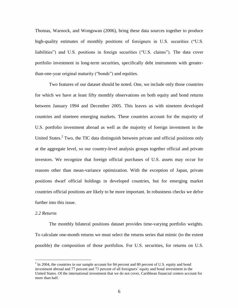
equities that ended in 2000 and re-emerged in 2003. This is shown in Figures 1 and 2.
The top panel in each figure shows year-over-year returns in equities and bonds; in both

16
the United States (Figure 1) and abroad (Figure 2), equity returns were generally higher
than bond returns from the beginning of the sample until 2000, and again from 2003 to
the end of the sample. The bottom panels of the two figures show equity weights from
actual portfolios (the thick lines) and theoretical 24-month buy-and-hold equity weights
(thin lines).8 A relationship clearly holds between relative performance for equities and
the actual weight on equities; while equities were outperforming bonds, investors (both
U.S. and foreign) allowed their portfolios to be more heavily weighted in equities.
Neither foreign nor U.S. investors seem to rebalance their portfolio when returns change
the portfolio weights of asset classes.
In order to distinguish between timing that is a result of a passive strategy versus
deliberate trading, we decompose the timing effect into trading and passive effects. Note
that the weight of asset j at the end of t-1 that would have resulted from a buy-and-hold
strategy adopted k periods ago can be calculated as follows:
where wj,t-1-k is the actual weight at the end of t-1-k. This weight is then updated
according to actual returns on asset j and returns on a buy-and-hold portfolio bh
pr .9 With
this we can decompose the timing effect into the part that depends on the deviations of
8 The buy-and-hold equity weight series begins only in January 1996 since it is the weight that foreigners
would have in equity had they not traded for twenty-four months starting in January 1994. 9 In order to construct the buy-and-hold weight at the end of t-1, we need the return on a buy-and-hold
portfolio in period t-1. This is not circular because the buy-and-hold portfolio return in t-1 uses buy-and-
hold weights from t-2.
1
,,1,,1, )1/()1(t
kt
bh
pjktj
bh
ktj rrww

17
actual weights from buy-and-hold weights and the part that depends on the deviation of
actual weights from average weights:
We call the first term on the right hand side the trading effect. It measures the
covariance between the deviations of actual weights from buy-and-hold weights and
subsequent returns. If investors tend to increase weights in assets that subsequently rise in
value, this term will be positive. We calculate this for both U.S. investors abroad and
foreign investors in the United States. We call the second term the passive effect. It
measures the covariance between the deviations of buy-and-hold weights from average
weights and subsequent returns. This covariance will tend to be positive if returns are
positively serially correlated.
Table V shows the foreign and U.S. trading effects as well as the passive effects.
Both trading and passive effects are calculated for different lags corresponding to
different buy-and-hold weights. For example, lag 6 uses buy-and-hold weights that would
have resulted from a buy-and-hold strategy adopted six months ago.
Panel A shows the results using all countries. The foreign trading effect is always
negative and statistically significant. The passive strategy effect is also always negative
and sometimes significant. This indicates that the negative foreign timing effect that we
documented in Table IV is due to poor passive strategy but mostly to ill-timed trading.
Foreign investors make new purchases (sales) that tend to be followed buy low (high)
returns. Interestingly, the foreign trading effect is negative and significant for both
N
j
tjj
bh
ktj
T
t
N
j
tj
bh
ktjtj
T
t
N
j
tjjtj
T
t
rwwT
rwwT
rwwT 1
,,1,
11
,,1,1,
11
,1,
1
)(1
)(1
)(1

18
developed and developing countries. Even though the overall timing effect in Table IV
was statistically significant only for developed countries, the part of the timing effect that
results from active trading is negative and significant in both developed and developing
countries. To the extent that we can interpret the negative trading effects as a lack of
investment skill, it appears to be low for investors from both developed and developing
counties. The magnitude of the effect is about 3 basis points per month at the 12-month
lag and 6 basis points at the 24-month lag. This translates to roughly 36 and 72 basis
points per year. In contrast, the U.S. trading effect is almost always positive although
never statistically significant.10
Poor timing on the part of foreign investors is apparent in Figure 1. For example,
in the twenty-four months after January 1994 U.S. equities outperformed U.S. bonds, so
the buy-and-hold weight for January 1996 is considerably higher than the actual weight
from January 1994 and the actual weight for January 1996. In fact, actual equity weights
are lower than the buy-and-hold weights for most of the second half of the 1990s. Putting
a relatively low weight on U.S. equity during the late 1990s turned out to have been a
poor decision, as U.S. equities performed spectacularly during this period. When U.S.
equities peaked in early 2000, foreigners‘ actual equity weights are higher than the buy-
and-hold weights, indicating that foreign investors were buying stocks (or selling
bonds)—in hindsight a poor decision. We see similarly poor timing toward the end of the
sample. During 2003 and 2004, foreign investors‘ weight in U.S. equity remains
relatively low despite the strong performance of the U.S. stock market. Had foreign
investors allowed their equity positions to appreciate in 2003, their equity weight (and the
10
This is entirely consistent with Thomas et al. (2006), who found that U.S. investors beat foreign
benchmarks not by skilled month-to-month trading but as a result of longer standing differences from
benchmark allocations.

19
return on their portfolio) would have been higher in 2004. Instead, foreign investors sold
U.S. equities or bought U.S. bonds when equities were about to outperform bonds.
Figure 2 allows a similar analysis for U.S. claims. In the late 1990s U.S.
investors‘ buy-and-hold weight is mostly lower than the actual equity weight. Therefore,
U.S. investors deliberately shifted toward equity while equity returns were relatively
high. U.S. investors continued to shift toward foreign equities even as foreign equities
were falling between 2000 and 2002. However, unlike foreign investors in the United
States, U.S. investors abroad appear to have deliberately shifted into equities before the
2003 and 2004 recovery in global equity markets. As the insignificant coefficients on the
U.S. trading effect in Table V show, in a statistical sense U.S. timing is neither poor nor
exceptional.
In Table VI we calculate the trading and passive effects for the aggregate private
positions in the United States. We find that foreign private positions also exhibit a
negative and statistically significant trading effect. This means that private foreign
investors tend to buy (sell) assets that subsequently experience low (high) returns. This is
further evidence that our aggregate results are not driven by mechanical accumulation of
dollar reserves but appear rather to be driven by the behavior of private investors.
3.4 Decomposition over 1994-1999 and 2000-2005 subsamples
In this subsection we investigate whether the decomposition of the returns
differential varies over time. Our aim is to determine which components of the returns
differential are stable over time and which vary. In part, this is motivated by the need to
understand the permanency or transitory nature of the returns differential (or lack of
thereof). In Table VII we split our sample into two periods: January 1994 through

20
December 1999, and January 2000 through December 2005. The table shows that the
composition and return effects switch signs between the two periods. For the return
effect, from 1994 through 1999 U.S. equities and bonds outperformed their foreign
counterparts, so the return effect is negative (that is, within each asset class foreign
investors earned more in the United States than U.S. investors earned abroad). The return
effect becomes positive during the period from 2000 through 2005, when both U.S.
equities and U.S. bonds performed worse than their foreign counterparts. As regards the
composition effect, from 1994 to 1999 it is positive; U.S. claims are weighted more
heavily toward equities than U.S. liabilities are and during this period equities
outperformed bonds. But between 2000 and 2005 both U.S. and foreign equities
performed far worse than bonds, so the composition effect becomes negative. Neither the
composition effect nor the return effect appears to be a permanent feature of U.S. external
positions.11
The transitory nature of composition and return effects is driven by volatile
returns. With volatile returns, timing of reallocations becomes more important. Table VII
shows that the foreign timing effect is negative during both time periods but is
statistically significant only in the 2000 to 2005 subperiod. As in the full sample, U.S.
timing remains statistically insignificant during both time periods. In Table VIII we
decompose the timing effect into the trading and passive effects. We see that at the 12-
and 24-month horizons the foreign trading effect is consistently negative and statistically
significant in both sub-samples. The magnitude of the trading effect is roughly the same
in the two sub-samples as in the full sample. Therefore, poor timing of new sales and
11
Of course, to the extent that over very long periods of time equities outperform bonds, we would expect
the composition effect to be positive.

21
purchases by foreign investors in the United States seems rather persistent. It is worth
emphasizing that the number of observations in the two sub-samples is relatively low.
Given this relatively small number of observations, the significance and the robustness of
the negative trading effect of foreign investors in the United States is striking. It suggests
that the poor timing found using the full sample represents a genuine difference in
investment style rather than bad luck on the part of foreign investors.
4. Conclusion
The goal of this paper was to improve our understanding of the sources of the
returns differential that the United States receives on its net international positions.
Consistent with existing literature we find that the greater weighting of U.S. portfolio
claims toward equity (compared to U.S. liabilities) contributes positively to the returns
differential. Over our sample period, however, this positive composition effect was offset
by a negative return effect as U.S. equities strongly outperformed foreign ones.
Importantly, we find that the poor timing of foreign investors‘ reallocations across stocks
and bonds lowered their return by 70 basis points per year, thus contributing positively to
the returns differential. While we find no evidence of superior market timing ability by
U.S. investors abroad, they do quite well relative to foreign investors in the United States.
For the current debate on global imbalances, it is important to know whether poor
foreign timing is permanent or transitory. Our estimate of poor foreign timing is stable
over our 12-year sample, but we have no confidence in its permanency. Increasing
financial integration, cross ownership of financial institutions, as well as improving

22
information flows suggest that any skill advantage is unlikely to persist.12
Should foreign
investors improve their timing, the U.S. external position would worsen at a faster pace.
Understanding why foreign investors consistently fail to anticipate shifts in
relative returns on different asset classes is an important question for future research. One
possibility is that foreign investors in the United States chase returns as suggested in
Bohn and Tesar (1996) and Brennan et al (2005). Superior U.S. investment skill is also
consistent with the evidence in Thomas et al. (2006), who find that U.S. investors‘
foreign equity portfolio outperforms capitalization-weighted benchmarks. It is also
possible that U.S. returns are less predictable than foreign returns, which would be
consistent with studies that find negative market timing among U.S. mutual funds (see,
for example, Ferson and Schadt 1996). Poor foreign timing in the U.S. is consistent with
Parwada, Walter, Winchester (2007) who, using proprietary trading data, find that foreign
investors incur higher transaction costs than domestic (U.S.) investors. It is also
consistent with Shukla and Inwegen (1995) who find that U.K. based mutual funds
investing in the U.S. perform worse than U.S. based mutual funds.
Another area for future research is foreign investors‘ reallocations within each
asset class. Currently, we are assuming that foreigners invest in market indices for both
equity and bonds, that is, we assume that foreign investors‘ allocation within each asset
class matches that of the benchmark index for each asset class. This assumption is on
solid footing, as security-level analysis of holdings suggests that at a point in time the
bulk of cross-border holdings is in just those securities that are in benchmark indices. But
if over time foreign investors‘ poor timing within asset classes is as poor as is their timing
12
For example, Dvorak (2005) finds that in Indonesia, U.S.-based global brokerages improve the
investment performance of both local and foreign investors.

23
between asset classes, then we underestimate the true magnitude of the timing and trading
effects.

24
References:
Ammer, J., S. Holland, D. Smith, and F. Warnock, 2006, Look at me now: The role of cross-
listings in attracting U.S. shareholders. NBER Working Paper 12500.
Bertaut, Carol C. and Ralph W. Tryon, 2007, Monthly estimates of U.S. cross-border securities
positions, Federal Reserve Board International Finance Discussion Paper # 910.
Bohn, H., and L. Tesar, 1996, U.S. equity investment in foreign markets: Portfolio rebalancing or
returns chasing? American Economic Review 86(2), 77-81.
Bosworth, Barry, Susan Collins, and Gabriel Chodorow-Reich, 2007, Returns on FDI: Does the
U.S. Really Do Better?, Brookings Trade Forum.
Burger, J., and F. Warnock, 2007, Foreign participation in local currency bond markets, Review
of Financial Economics 16, 291-304.
Brennan, Michael J., H. Henry Cao, Norman Strong and Xinzhong Xu, 2005, The dynamics of
international equity market expectations, Journal of Financial Economics 77, 257–288.
Curcuru, Stephanie E., Tomas Dvorak, and Francis E. Warnock, 2008, Cross-Border Returns
Differentials, Quarterly Journal of Economics (forthcoming).
Choe, Hyuk, Bong-Chan Kho, and René M. Stulz, 2005, Do Domestic Investors Have an Edge?
The Trading Experience of Foreign Investors in Korea, Review of Financial Studies
18(3):795-829.
Devereux, Michael B. and Makoto Saito, 2006. A Portfolio Theory of International Capital
Flows, Institute for International Integration Studies Discussion Paper No. 124.
Dvorak, Tomas, 2005. Do domestic investors have an information advantage? Evidence from
Indonesia, Journal of Finance 60, 817-839.
Engel, Charles and Akito Matsumoto, 2006, Portfolio Choice in a Monetary Open-Economy
DSGE Model, working paper.
Ferson, Wayne, and Kenneth Khang, 2002, Conditional performance measurement using
portfolio weights: Evidence for pension funds, Journal of Financial Economics 65, 249-
282.
Ferson, W. and R. Schadt, 1996, Measuring fund strategy and performance in changing economic
conditions, Journal of Finance 51(2), 425-461.
Forbes, Kristin J., 2007. Global Imbalances: A Source of Strength or Weakness?, Cato Journal
27, 193-202.
Forbes, Kristin J., 2008. Why Do Foreigners Invest in the United States? working paper.
Gourinchas, Pierre-Olivier and Helene Rey, 2007, From world banker to world venture capitalist:
The U.S. external adjustment and the exorbitant privilege, in R. Clarida (ed.) G7 Current

25
Account Imbalances: Sustainability and Adjustment (Chicago, University of Chicago
Press), 11-55.
Griever, W., G. Lee, and F. Warnock, 2001, The U.S. system for measuring cross-border
investment in securities: A primer with a discussion of recent developments. Federal
Reserve Bulletin 87(10), 633-650.
Grinblatt, Mark and Sheridan Titman, 1993, Performance measurement without benchmarks: An
examination of mutual fund returns, Journal of Business 66, 47-68.
Gros, Daniel, 2006, Why the U.S. Current Account Deficit is Not Sustainable, International
Finance 9(2), 241-260.
Heath, A., 2007, What explains the U.S. net income balance? BIS Working Papers No 223.
Higgins, Matthew, Thomas Klitgaard and Cedric Tille, 2007, Borrowing without debt?
Understanding the U.S. international investment position, Business Economics 42(1).
Hung, J., and A. Mascaro, 2004, Return on cross-border investment: Why does U.S. investment
abroad do better? CBO Technical Paper Series 2004-17.
Kho, B.-C., R. Stulz, and F. Warnock, 2006, Financial globalization, governance, and the
evolution of the home bias. NBER Working Paper 12386.
Lane, Philip R., and Gian Maria Milesi-Ferretti, 2005, Financial Globalization and Exchange
Rates, IMF working paper # 05/3.
Parwada, Jerry T., Terry S. Walter and Donald W. Winchester, 2007, Do foreign investors pay
more for stocks in the United States? An analysis by country of origin, working paper.
Shukla, Ravi K. and Gregory B. van Inwegen, 1995, Do locals perform better than foreigners?:
An analysis of UK and US mutual fund managers, Journal of Economics and Business 47,
241-253.
Thomas Charles P., Francis E. Warnock and Jon Wongswan, 2006, The performance of
international equity portfolios, NBER Working Paper 12346.
Tille, Cedric, and Eric van Wincoop, 2007, International capital flows, NBER Working Paper
12856.
Warnock, F. and V. Warnock, 2006, International capital flows and U.S. interest rates. NBER
Working Paper 12560.

26
Table I
Country Composition of U.S. Portfolio of Foreign Equity and Foreign Bonds Country‘s weight in U.S. equity (bond) portfolio is the U.S. equity (bond) position in the country divided
by the total U.S. equity (bond) position in all 38 countries included in the sample. Country‘s equity return is
the average of simple monthly returns on MSCI gross U.S. dollar total return index expressed in percent.
Developed countries‘ bond returns are the weighted averages of simple monthly U.S. dollar returns on the
country‘s MSCI bond index and the MSCI Eurodollar Credit index where the weights on the Eurodollar
index are the shares of dollar denominated bonds in U.S. holdings of foreign bonds. Emerging markets‘
bond returns are simple monthly returns on the EMBI+ U.S. dollar index. The time period is from January
1994 through December 2005 unless otherwise noted in the last column.
Country
Country‘s Avg.
Weight in U.S.
Equity Portfolio
Country‘s Avg.
Equity Return
Country‘s Avg.
Weight in U.S.
Bond Portfolio
Country‘s
Avg. Bond
Return
Country
Included
from
Australia 0.030 1.076 0.037 0.567 Jan ‗94
Austria 0.003 0.939 0.005 0.598 Jan ‗94
Belgiumlux 0.010 1.078 0.022 0.597 Jan ‗94
Canada 0.071 1.225 0.227 0.574 Jan ‗94
Denmark 0.006 1.239 0.016 0.649 Jan ‗94
Finland 0.023 2.023 0.009 0.600 Jan ‗94
France 0.076 0.964 0.049 0.573 Jan ‗94
Germany 0.056 0.896 0.092 0.565 Jan ‗94
Greece 0.002 1.346 0.003 0.720 Jun ‗97
Ireland 0.013 0.971 0.010 0.651 Jan ‗94
Italy 0.029 1.165 0.036 0.750 Jan ‗94
Japan 0.158 0.329 0.072 0.262 Jan ‗94
Netherlands 0.081 0.969 0.051 0.565 Jan ‗94
Norway 0.007 1.226 0.010 0.639 Jan ‗94
Portugal 0.003 0.923 0.002 0.701 Jan ‗94
Spain 0.024 1.343 0.018 0.689 Jan ‗94
Sweden 0.026 1.505 0.025 0.698 Jan ‗94
Switzerland 0.055 1.055 0.002 0.544 Jan ‗94
U. K. 0.213 0.813 0.136 0.618 Jan ‗94
Argentina 0.006 1.112 0.029 -0.347 Jan ‗94
Brazil 0.018 1.966 0.027 0.622 Jan ‗94
Chile 0.003 0.965 0.010 0.223 Jun ‗99
China 0.003 -0.086 0.004 0.152 Apr ‗94
Colombia 0.000 1.857 0.006 0.209 Mar ‗97
Hungary 0.002 2.225 0.001 -0.019 Feb ‗99
India 0.006 0.994 0.001 0.095 Mar ‗96
Korea 0.019 1.458 0.015 0.057 Jan ‗94
Malaysia 0.007 0.333 0.007 0.148 Nov ‗96
Mexico 0.026 1.202 0.050 0.225 Jan ‗94
Morocco 0.000 0.980 0.001 0.332 Jan ‗95
Peru 0.001 1.618 0.002 0.994 Jan ‗94
Philippine 0.003 -0.127 0.006 0.213 Jan ‗94
Poland 0.001 1.063 0.003 0.467 Jan ‗94
Russia 0.004 3.406 0.007 1.393 Jan ‗95
South Africa 0.009 1.267 0.004 0.248 Jun ‗94
Thailand 0.005 0.331 0.004 0.130 Jun ‗97
Turkey 0.002 2.167 0.003 0.355 Jul ‗96
Venezuela 0.001 1.319 0.010 0.632 Jan ‗94

27
Table II
Characteristics of U.S. Foreign Claims and Liabilities Equity weight in U.S. claims is the share of foreign equities in U.S. investors‘ foreign bond and equities
portfolio. Equity weight in U.S. liabilities is the share of U.S. equities in foreign investors‘ U.S. bond and
equities portfolio. Returns on U.S. equities are the monthly simple returns on the U.S. MSCI gross return
equity index. Returns on U.S. bonds are foreign-portfolio-weighted averages of Lehman Brothers Treasury,
Corporate and Agency bond indices. Returns on foreign equities are U.S.-portfolio-weighted averages of
each country‘s simple monthly dollar return on its MSCI gross return equity index. Returns on foreign
bonds are U.S.-portfolio-weighted averages of each country‘s bond returns. Developed countries‘ bond
returns are the weighted averages of simple monthly U.S. dollar returns on the country‘s MSCI bond index
and the MSCI Eurodollar Credit index where the weights on the Eurodollar index are the shares of dollar
denominated bonds in U.S. holdings of foreign bonds. Emerging markets‘ bond returns are simple monthly
returns on the EMBI+ U.S. dollar index. All data are from January 1994 through December 2005, unless
otherwise noted in Table I.
Mean Median St.Dev. Min Max
Panel A: Equity Weight in U.S. Claims (%)
All Countries 70.8 71.1 3.8 62.7 78.3
Developed Countries 72.3 72.7 4.5 62.1 81.1
Emerging Markets 60.2 60.6 6.7 44.9 75.9
Panel B: Equity Weight in U.S. Liabilities (%)
All Countries 41.7 39.4 5.9 33.9 54.4
Developed Countries 45.8 42.8 6.0 39.0 59.1
Emerging Markets 9.0 9.4 2.8 4.0 14.5
Panel C: Equity Returns (% per month)
Return on U.S. Equities 0.940 1.318 4.306 -13.905 9.984
Return on Foreign Equities
All Countries 0.766 1.221 4.321 -14.791 10.726
Developed Countries 0.797 1.068 4.169 -13.004 10.540
Emerging Markets 0.849 2.181 7.433 -32.656 16.408
Panel D: Bond Returns (% per month)
Return on U.S. Bonds
By All Countries 0.478 0.576 0.922 -2.769 2.957
By Developed Countries 0.484 0.594 0.954 -2.948 3.013
By Emerging Markets 0.451 0.481 0.794 -2.123 2.502
Return on Foreign Bonds
All Countries 0.493 0.511 1.620 -4.641 5.528
Developed Countries 0.567 0.451 1.605 -3.558 5.149
Emerging Markets 0.197 0.716 3.798 -22.812 8.822

28
Table III
Returns Differential on U.S. Claims and Liabilities This table shows average percent returns using the monthly bond and equity portfolios for the
time period January 1994 to December 2005.
Equity All Countries Developed Countries Emerging Markets
Claims 0.766 0.797 0.849
Liabilities 0.940 0.940 0.940
Differential -0.174 -0.143 -0.091
Bonds
Claims 0.493 0.567 0.197
Liabilities 0.478 0.484 0.451
Differential 0.015 0.083 -0.254
Combined Bonds and Equity
Claims 0.668 0.712 0.599
Liabilities 0.612 0.627 0.489
Differential 0.056 0.084 0.110

29
Table IV
Decomposition of the Returns Differential into Composition, Return and Timing Effects
Difference, the difference between the average monthly percentage return on the portfolio of U.S.
claims (foreign equities and U.S. bonds) and the return on U.S. liabilities (U.S. equities and U.S.
bonds), equals Composition Effect plus Return Effect minus Foreign Timing Effect plus U.S.
Timing Effect. The composition, return and timing effects are defined in section 2.1. Standard t-
statistics are in parentheses. Bootstrapped z-statistics based on 1000 draws are in brackets.
Statistical significance at the 1, 5, and 10 percent levels are denoted by ***, **, and *,
respectively.
Difference
(claims-liabilities) Composition Effect Return Effect
Timing Effects
Foreign U.S.
Panel A: All Countries
0.056 0.107 -0.091 -0.058** -0.018
(0.31) [1.07] [-0.60] (-2.67) (-1.48)
Panel B: Vis-à-vis Private Foreign Positions
-0.002 0.074 -0.112 -0.053** -0.018
(-0.01) [1.12] [-0.62] (-2.67) (-1.44)
Panel C: Developed Countries
0.084 0.091 -0.050 -0.065** -0.022
(0.48) [1.00] [-0.33] (-2.97) (-1.46)
Panel D: Emerging Market Countries
0.11 0.292 -0.197 -0.006 0.009
(0.25) [1.45] [-0.60] (-0.72) (0.27)

30
Table V
Decomposing the Timing Effect into Trading and Passive Effects The covariance between lagged weights and returns (the timing effect) is decomposed into (1) the
covariance between lagged deviations of actual from buy-and-hold weights and subsequent returns (the
trading effect), and (2) the covariance of the lagged deviation of buy-and-hold weights from average
weights and subsequent returns. Lag indicates the horizon of the buy-and-hold weight in months. T-
statistics are in parentheses. Statistical significance at the 1, 5, and 10 percent levels are denoted by ***, **,
and *, respectively.
Lag Foreign Timing Effect U.S. Timing Effect # of
obs Trading Effect Passive Effect Trading Effect Passive Effect
Panel A: All Countries
6 -0.011**
(-2.03)
-0.049**
(-2.45)
0.003
(0.69)
-0.019
(-1.57) 138
12 -0.034***
(-3.38)
-0.029
(-1.59)
0.000
(0.05)
-0.016
(-1.34) 132
24 -0.061***
(-3.48)
-0.001
(-0.03)
-0.003
(-0.37)
-0.015
(-1.04) 120
Panel B: Developed Countries
6 -0.011*
(-1.93)
-0.057***
(-2.85)
0.004
(0.99)
-0.023
(-1.56) 138
12 -0.032***
(-3.17)
-0.038**
(-2.15)
0.003
(0.61)
-0.022
(-1.51) 132
24 -0.059***
(-3.31)
-0.007
(-0.37)
0.006
(1.10)
-0.028*
(-1.71) 120
Panel C: Emerging Market Countries
6 -0.007*
(-1.91)
0.001
(0.12)
0.013
(0.93)
-0.009
(-0.23) 138
12 -0.021***
(-3.34)
0.013
(1.29)
0.023
(1.19)
-0.019
(-0.44) 132
24 -0.029**
(-2.39)
0.018
(1.07)
-0.016
(-0.67)
0.029
(0.62) 120

31
Table VI
Trading and Passive Effects of Aggregate Foreign Private Investors in the U.S.
The calculations in this table use aggregate private foreign positions in the U.S. The covariance
between lagged weights and returns (the timing effect) is decomposed into (1) the covariance
between lagged deviations of actual from buy-and-hold weights and subsequent returns (the
trading effect), and (2) the covariance of the lagged deviation of buy-and-hold weights from
average weights and subsequent returns. Lag indicates the horizon of the buy-and-hold weight in
months.. T-statistics are in parentheses. Statistical significance at the 1, 5, and 10 percent levels
are denoted by ***, **, and *, respectively.
Foreign Private Timing Effect # of
Lag Trading Effect Passive Effect obs
6 -0.013**
(-2.45)
-0.042**
(-2.26) 138
12 -0.032***
(-3.58)
-0.024
(-1.42) 132
24 -0.058***
(-3.49)
0.003
(0.11) 120

32
Table VII
Decomposition of the Returns Differential into Composition, Return and Timing Effects:
Subsamples
Difference, the difference between the average monthly percentage return on the portfolio of U.S.
claims (foreign equities and U.S. bonds) and the return on U.S. liabilities (U.S. equities and U.S.
bonds), equals Composition Effect plus Return Effect minus Foreign Timing Effect plus U.S.
Timing Effect. The composition, return and timing effects are defined in section 2.1. Standard t-
statistics are in parentheses. Bootstrapped z-statistics based on 1000 draws are in brackets.
Statistical significance at the 1, 5, and 10 percent levels are denoted by ***, **, and *,
respectively.
Difference
(claims-liabilities) Composition Effect Return Effect
Timing Effects
Foreign U.S.
Panel A: 1994 -1999
-0.127 0.304*** -0.452** -0.009 0.012
(-0.41) [3.01] [-2.14] (-0.39) -0.83
Panel B: 2000 – 2005
0.239 -0.115 0.279 -0.106*** -0.032
(0.92) [-0.74] [1.46] (-2.88) (-1.58)

33
Table VIII
Decomposing the Timing Effect into Skill and Passive Strategy: Subsamples The covariance between lagged weights and returns (the timing effect) is decomposed into (1) the
covariance between lagged deviations of actual from buy-and-hold weights and subsequent returns (the
trading effect), and (2) the covariance of the lagged deviation of buy-and-hold weights from average
weights and subsequent returns. Lag indicates the horizon of the buy-and-hold weight in months. T-
statistics are in parentheses. Statistical significance at the 1, 5, and 10 percent levels are denoted by ***, **,
and *, respectively.
Lag Foreign Timing U.S. Timing
Nobs Trading Effect Passive Effect Trading Effect Passive Effect
Panel A: 1994 -1999
6 -0.013
(-1.74)
0.004
(0.18)
0.008
(1.29)
0.010
(0.65) 66
12 -0.037***
(-2.53)
0.029
(1.37)
0.011
(1.22)
0.012
(0.70) 60
24 -0.071**
(-2.25)
0.080*
(2.10)
0.015*
(1.64)
0.011
(0.56) 48
Panel B: 2000-2005
6 -0.011
(-1.19)
-0.095***
(-3.06)
-0.003
(-0.55)
-0.029
(-1.36) 66
12 -0.030*
(-1.94)
-0.054***
(-2.77)
-0.009
(-1.00)
-0.014
(-0.62) 60
24 -0.047*
(-2.06)
-0.013
(-0.57)
-0.007
(-0.51)
-0.008
(-0.21) 48

34
Figure 1
U.S. equity and bond returns and the equity weight in U.S. portfolio liabilities The 12-month total return on U.S. equities is the return on the MSCI U.S. total return index. The 12-month
total return on U.S. bonds is the foreign-portfolio-weighted average of Lehman Brothers Treasury,
Corporate and Agency bond returns. Actual equity weight in U.S. portfolio liabilities is the share of U.S.
equities in foreign investors‘ U.S. bond and equities portfolio. The 24-month buy-and-hold weight is the
share of equity that would have resulted from a buy-and-hold strategy adopted 24 months ago.
U.S.equities
U.S. bonds
-20
02
04
06
0
12
-mo
nth
to
tal re
turn
(%
pe
r ye
ar)
actualweight
24-monthbuy-and-hold
weight
.35
.4.4
5.5
.55
eq
uity w
eig
ht
in U
.S.
po
rtfo
lio
lia
bilitie
s
1994 1995 1996 1997 1998 1999 2000 2001 2002 2003 2004 2005 2006

35
Figure 2
Foreign equity and bond returns and the equity weight in U.S. portfolio claims The 12-month total return on foreign equities is the U.S.-portfolio-weighted average of each country‘s
dollar return on its MSCI gross return equity index. The 12-month total returns on foreign bonds are U.S.-
portfolio-weighted averages of each country‘s bond returns. Developed countries‘ bond returns are the
weighted averages of simple monthly U.S. dollar returns on the country‘s MSCI bond index and the MSCI
Eurodollar Credit index where the weights on the Eurodollar index are the shares of dollar denominated
bonds in U.S. holdings of foreign bonds. Emerging markets‘ bond returns are simple monthly returns on the
EMBI+ U.S. dollar index. foreign bonds is the U.S.-portfolio-weighted average of the MSCI (for developed
countries) or EMBI+ (for emerging markets) bond return indices. Actual equity weight in U.S. claims is the
share of foreign equities in U.S. investors‘ foreign bond and equities portfolio. The 24-month buy-and-hold
weights is the share of equity that would have resulted from a buy-and-hold strategy adopted 24 months
ago.
foreignequities
foreignbonds
-20
02
04
06
0
12
-mo
nth
to
tal re
turn
(%
pe
r ye
ar)
actualweight
24-monthbuy-and-hold
weight
.6.6
5.7
.75
eq
uity w
eig
ht
in U
.S.
po
rtfo
lio
asse
ts
1994 1995 1996 1997 1998 1999 2000 2001 2002 2003 2004 2005 2006