One Too Many Red Solo Cups proofread-2

One Too Many Red Solo Cups! 2015

DOES A BEER TAX REDUCE YOUTH DRUNK DRIVING FATALITIES

bY: Tyler Collins

1

Abstract

If the cost of alcohol reduces the consumption of the beverage, does a hike in the price of

alcohol, caused by an alcohol tax reduce the drunk driving fatalities? This paper explores the

origins of alcohol control and touches on the different aspects of prevention. Special

consideration is given to how alcohol policies effect underage alcohol driving fatalities.

2

Introduction

“Alcohol intoxication increases the risk of injury resulting from motor vehicle crashes

and violent assaults.” (Holder, et al. (2000) Every year, thousands of people die in motor vehicle

crashes and a substantial portion of those accidents are alcohol related. Since before prohibition,

the government and citizens have grappled with how to manage a substance that is infamously

difficult to manage.

Citizen advocacy groups such as, “MADD (Mothers Against Drunk Driving), RID

(Remove Intoxicated Drivers), SADD (Students Against Drunk Driving), and others launched

grassroots campaigns against alcohol-impaired driving in the late 1970s and early 1980s”

(Roizen, 2004, p. 68). Since that time, the knowledge surrounding alcohol and how it affects our

everyday lives has changed exponentially. The marketing campaigns that focused largely on

alcoholics have refocused their efforts to all consumers. “Alcohol problems arise, not from a

small group of chronic dependents, but from the drinking habits of the general population”

(Moore & Gerstein, 1981, p. 13).

Not all drinkers are the same; however, “Alcohol's effect on individuals stems from a

variety of cognitive, biological, and social factors. The propensity to binge drink may arise from

a combination of these factors, which could contribute to the underlying “cause” of binge

drinking” (Courtney & Polich, 2009). With all of these factors in play, it is only logical that to

combat the misuse of alcohol, policy makers must find a way to control the behavior of drinkers

across a broad spectrum of personal qualities.

“The most fundamental law of economics links the price of a product to the demand for

that product. Accordingly, increases in the monetary price of alcohol (i.e., through tax increases)

3

would be expected to lower alcohol consumption and its adverse consequences” (Chaloupka,

Grossman, & Saffer, 2002, para. 1). Approaching alcohol consumption with this logic, “the study

found consistent evidence that increases in the price of alcohol resulting from higher monetary

prices significantly reduced the number of alcoholic drinks consumed by young adults in the past

year. Moreover, the analyses provided strong evidence that drinking in this age group is

addictive in the sense that a strong interdependency existed among past, current, and future

alcohol consumption” (Chaloupka, Grossman, & Saffer, 2002, para.2).

Purpose of the Study

“Alcohol policy is one of the severest tests of government’s will to serve the public

interest” (Stockwell, 2004, p. 1090). With alcohol affecting violent crime, personal health, and a

flood of drunk-driving deaths, it is only natural that the government and public interest groups

will try to work for the common good. According to Hanssens & Ornsteing (1985), “Alcohol

control laws can be divided into three general categories: (1) economic legislation directed at

raising revenues for the state and/or protecting sellers from competition, (2) attempts to control

the social costs resulting from excessive drinking, and (3) attempts to prevent product

adulteration and false advertising” (p. 201). This study is going to focus on the first category,

economic legislation. “Studies suggest that increases in federal or state excise taxes on alcohol

discourage heavy drinking and reduce motor vehicle fatalities” (Brown, Jewell, and Richer,

1996, p. 1043).

Background Literature

Robert Reynolds 1984 paper, “Toward the Prevention of Alcohol Problems Government,

Business and Community Action” talks about the three aspects of prevention. “The first was to

affect the terms and conditions under which alcohol is available, through special taxes, minimum

4

age requirements, regulation of outlets and availability and times of sale-all the things that

determine how easy and convenient it is for people to have access to alcohol” (Reynolds, 1984,

p. 3). This paper focuses on the aspect of prevention in regard of special taxes. “The second idea

was to shape drinking practices directly by talking to people about what constitutes safe and

appropriate drinking behavior” (Reynolds, 1984, 3). “The third idea was to make the

environment a safer one in which to be drunk” (Reynolds, 1984, 3). This might include

suggestions like making for sure taxi services are available.

Reynolds’ aspects of prevention concur with other academics in this field, especially

when businesses are part of the prevention of alcohol misuse. Levine & Reinarman’s paper,

From Prohibition to Regulation: Lessons from Alcohol Policy for Drug Policy states,

Under alcohol control, all establishments licensed for on-premises consumption of

spirits were specifically restricted in ways that shaped the cultural practice of

drinking. In some areas, control laws attempted to moderate the effects of

drinking by encouraging food consumption (just as hosts of cocktail parties

served hors d’oeuvres). For example, spirit sales often were limited to bona fide

restaurants with laws specifying how many feet of kitchen space and how many

food preparation workers there must be. Most states established restrictions on the

number of entrances and their locations (back entrances are usually prohibited);

the times of day and days of the week when sales may occur; permissible

decorations; degree of visibility of the interior from the street; numbers and uses

of other rooms; distance of the establishment from churches, schools, and other

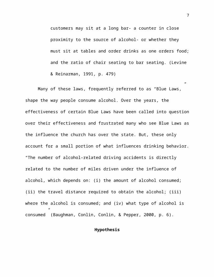
alcohol outlets; whether customers may sit at a long bar- a counter in close

5

proximity to the source of alcohol- or whether they must sit at tables and order

drinks as one orders food; and the ratio of chair seating to bar seating. (Levine &

Reinarman, 1991, p. 479)

Many of these laws, frequently referred to as “Blue Laws,” shape the way people

consume alcohol. Over the years, the effectiveness of certain Blue Laws have been called into

question over their effectiveness and frustrated many who see Blue Laws as the influence the

church has over the state. But, these only account for a small portion of what influences drinking

behavior. “The number of alcohol-related driving accidents is directly related to the number of

miles driven under the influence of alcohol, which depends on: (i) the amount of alcohol

consumed; (ii) the travel distance required to obtain the alcohol; (iii) where the alcohol is

consumed; and (iv) what type of alcohol is consumed” (Baughman, Conlin, Conlin, & Pepper,

2000, p. 6).

Hypothesis

This paper’s theoretical derived hypothesis comes from an “increases in the price of

alcohol resulting from higher monetary prices significantly reduced the number of alcoholic

drinks consumed by young adults” (Chaloupka, Grossman, & Saffer, 2002, para. 2).

Method

The data for this paper is gathered from multiple sources. State level data regarding drunk

driving is gathered from (Responsibility.org). This source gives the percentage of total fatalities

in the state from drunk-driving automobile accidents divided by all automobile fatalities

(PERCTFATAL) and the percentage of total under 21 fatalities in the state from drunk-driving

automobile accidents, divided by all under 21 automobile fatalities (PERCT21). The data can be

6

viewed in the form of a sitemap which draws on data from the Center for Disease Control and

Prevention.

State level data for consumption comes from (State-Specific Alcohol Consumption Rates

for 2013). The data includes, “State-Specific Weighted Prevalence Estimates of Alcohol Use and

Binge Drinking Among Women 18–44 Years of Age.” The code for any use is (ANYDRK) and

the code for binge drinking rates is (BINGE). Any use is defined as “any drink within the past 30

days” and binge drinking is defined as “4 or more drinks at any given time during the last 30

days.”

State level data for the taxes of alcohol come from The Tax Policy Center (Alcohol Rates

2000-2010, 2013-2015). The variables are divided into three categories, beer tax (BEERTAX),

wine tax (WINETAX), and liquor tax (LIQTAX). The variables reflect the dollar amount of tax

specified by beverage.

Finally, the paper uses state level data to get the number of miles driven a year in each

state and the population of each state to get the total miles driven adjusted for population by

state. To do this, the number of miles driven each year is illustrated per billion and gathered from

the United States Census (State and Local Areas, 2010) and is divided by the population of each

state, which is gathered from the United States Census (Quick Facts, 2010) to give us the new

variable of the population adjusted miles driven coded as (WEIGHTMILES).

7

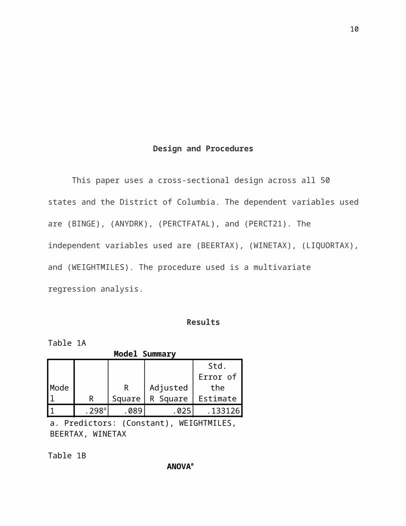
Design and Procedures

This paper uses a cross-sectional design across all 50 states and the District of Columbia.

The dependent variables used are (BINGE), (ANYDRK), (PERCTFATAL), and (PERCT21).

The independent variables used are (BEERTAX), (WINETAX), (LIQUORTAX), and

(WEIGHTMILES). The procedure used is a multivariate regression analysis.

Results

Table 1AModel Summary

Model R R SquareAdjusted R

SquareStd. Error of the Estimate

1 .298a .089 .025 .133126a. Predictors: (Constant), WEIGHTMILES, BEERTAX, WINETAX

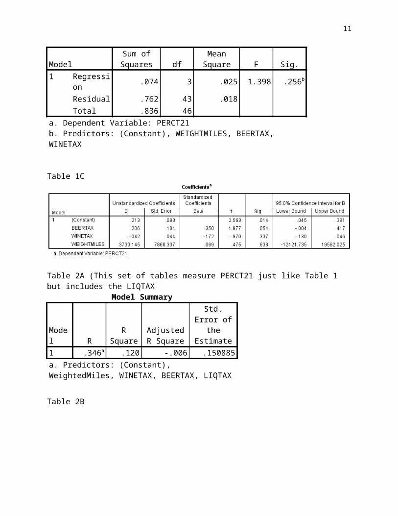
Table 1BANOVAa

ModelSum of Squares df Mean Square F Sig.

1 Regression .074 3 .025 1.398 .256b

Residual .762 43 .018Total .836 46

a. Dependent Variable: PERCT21b. Predictors: (Constant), WEIGHTMILES, BEERTAX, WINETAX

Table 1C

8

Table 2A (This set of tables measure PERCT21 just like Table 1 but includes the LIQTAXModel Summary



1 .346a .120 -.006 .150885a. Predictors: (Constant), WeightedMiles, WINETAX, BEERTAX, LIQTAX

Table 2B

Table 2C


9



1 .303a .092 -.043 .055032a. Predictors: (Constant), WeightedMiles, BEERTAX, LIQTAX, WINETAX

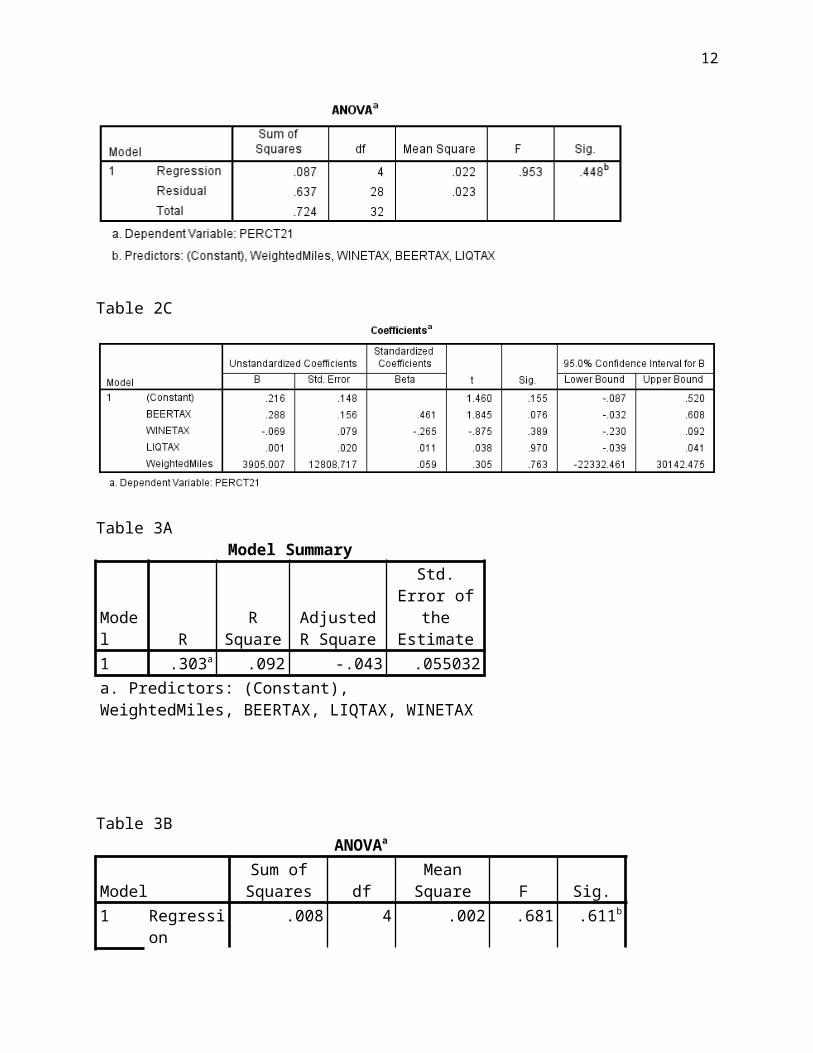
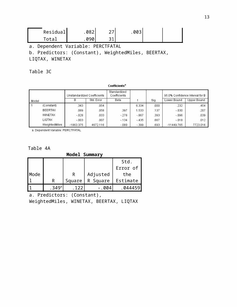
Table 3BANOVAa


1 Regression .008 4 .002 .681 .611b

Residual .082 27 .003Total .090 31

a. Dependent Variable: PERCTFATALb. Predictors: (Constant), WeightedMiles, BEERTAX, LIQTAX, WINETAX

Table 3C




1 .349a .122 -.004 .044459a. Predictors: (Constant), WeightedMiles, WINETAX, BEERTAX, LIQTAX

10

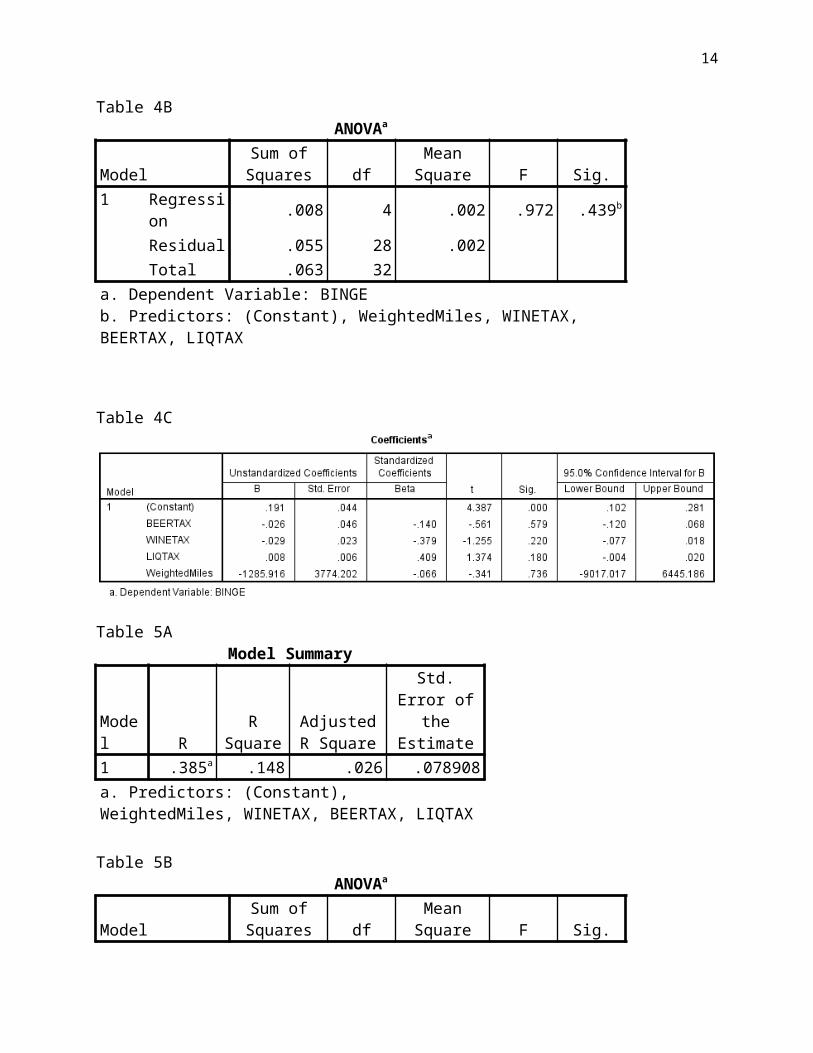
Table 4BANOVAa


1 Regression .008 4 .002 .972 .439b

Residual .055 28 .002Total .063 32

a. Dependent Variable: BINGEb. Predictors: (Constant), WeightedMiles, WINETAX, BEERTAX, LIQTAX

Table 4C




1 .385a .148 .026 .078908a. Predictors: (Constant), WeightedMiles, WINETAX, BEERTAX, LIQTAX

Table 5B

11

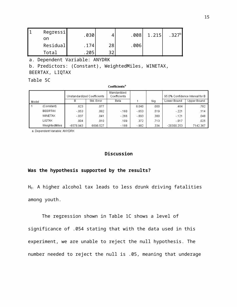
ANOVAa


1 Regression .030 4 .008 1.215 .327b

Residual .174 28 .006Total .205 32

a. Dependent Variable: ANYDRKb. Predictors: (Constant), WeightedMiles, WINETAX, BEERTAX, LIQTAX

Table 5C

Discussion

Was the hypothesis supported by the results?

HO: A higher alcohol tax leads to less drunk driving fatalities among youth.

The regression shown in Table 1C shows a level of significance of .054 stating that with

the data used in this experiment, we are unable to reject the null hypothesis. The number needed

to reject the null is .05, meaning that underage automobile accidents are not significantly reduced

by a higher beer tax.

While the effect of a beer tax almost reaches statistical significance, a wine or liquor tax

doesn’t even come close. This is probably because beer is the most popular and easily accessible

beverage among youth.

12

Why might the results have turned out that way?

As mentioned earlier, the consumption data was “State-Specific Weighted Prevalence

Estimates of Alcohol Use and Binge Drinking Among Women 18–44 Years of Age.” (State-

Specific Alcohol Consumption Rates for 2013) This excludes any data regarding the

consumption of alcohol among men. “Higher volumes of high alcohol content beer, wine and

distilled spirits were purchased in the licensed hotels during late trading hours. Extended hours

were also associated with young crowds, more likely to be women, and lower blood alcohol

levels among women but not men” (Popova, Giesbrecht, Bekmuradov, Javadeep, 2009, p. 513).

This gives me the reason to believe that when the data that includes male consumption is

introduced, the null hypothesis will be able to be rejected.

How could the study be improved?

One way the study could be improved would be to add the consumption data among

males. Other data that could be included would be the percentage of each ethnicity represented

by state to see how drinking behaviors change between different groups. The religious affiliation

of individuals by state and the average distance driven to obtain the alcohol could also provide

valuable data for this study.

Another way the study could be improved, would be to include other types of alcohol

taxes than the current ones given. There are other alcohol taxes and they vary by state, county,

and city. Including these in the study and finding a way to properly measure the other tax options

available may have an impact.

13

14

References

Baughman, R., Conlin, S., Conlin, M., Pepper, J., (2000). Slippery when wet: The effects of local alcohol access laws on highway safety. Center for Policy Research, 1-28.

Brown, R., Jewell, R., Richer, J., (1996) Endogenous alcohol prohibition and drunk driving. Southern Economic Association, 62(4), 1043-1053.

Chaloupka, F., Grossman, M., & Saffer, H. (2002, August 1). The Effects of Price on Alcohol Consumption and Alcohol-Related Problems. Retrieved October 6, 2015, from http://pubs.niaaa.nih.gov/publications/arh26-1/22-34.htm

Courtney, K. E., & Polich, J. (2009). Binge drinking in young adults: Data, definitions, and determinants. Psychological Bulletin, 135(1), 142–156. http://doi.org/10.1037/a0014414

Hanssens, D., Ornstein., (1985). Alcohol control laws and the consumption of distilled spirits and beer. Journal of Consumer Research, The University of Chicago Press, 12(2)

Holder, H., Gruenewald, P., Ponicki,W., Treno, Andrew., Grube, J., Saltz, R., Voas, R., Reynolds, R., Davis, J., Sanches, L., Gaumont, G., Roeper, R., (2000). “Effect of community-based interventions on high-risk drinking and alcohol-related injuries. JAMA, 284(18), 2341-2347.

Levine, H., & Reinarman, C. (1991). From prohibition to regulation: Lessons from alcohol policy for drug policy. The Milbank Quarterly,461-494.

Moore, M., & Gerstein, Dean, (1981). Alcohol and public policy: Beyond the shadow of prohibition” National Academy Press, 3-463.

Popova, S., Giesbrecht, N., Bekmuradov, D., Patra, Jayadeep., (2009) “EPIDEMIOLOGY AND POLICY: Hours and days of sale and density of alcohol outlets: Impacts on alcohol consumption and damage; a systematic review.” Alcohol & Alcoholism, 44(5), 500-516.

Reynolds, Robert., (1984). Toward the prevention of alcohol problems government, business, and community action. National Institute on Alcohol Abuse and Alcoholism, 137-144 .

Roizen, R. (2004). “How does the nation’s alcohol problem change from era to era? Stalking the social logic of problem-definition transformations since Repeal.” University of Massachusetts Press. 61-87

15

Stockwell, Tim., (2004). Addiction “Lies, Damned Lies And No Statistics: A study of Dysfunctional Democracy in Action” Vol. 99, Issue 9, 1090-1091.

DATA:

Alcohol Rates 2000-2010, 2013-2015. (2015, February 16). Retrieved October 7, 2015, from http://www.taxpolicycenter.org/taxfacts/displayafact.cfm?Docid=349

States & Local Areas. (2010). Retrieved October 7, 2015. www.census.gov/compendia/databooks

State-Specific Alcohol Consumption Rates for 2013. (2015, September 24). Retrieved October 7, 2015. http://www.cdc.gov/ncbddd/fasd/monitor_table.html

Quick Facts. (2010). Retrieved October 7, 2015 http://quickfacts.census.gov/qfd/states/11000.html

Responsibility.org - Fighting Drunk Driving & Underage Drinking: Foundation for Advancing Alcohol Responsibility. (2015). Retrieved October 7, 2015.

Documents

One Too Many Red Solo Cups proofread-2