Embed Size (px)
Citation preview
AN-922APPLICATION NOTE
One Technology Way • P.O. Box 9106 • Norwood, MA 02062-9106, U.S.A. • Tel: 781.329.4700 • Fax: 781.461.3113 • www.analog.com
Digital Pulse-Shaping Filter Basics
by Ken Gentile
Rev. 0 | Page 1 of 12
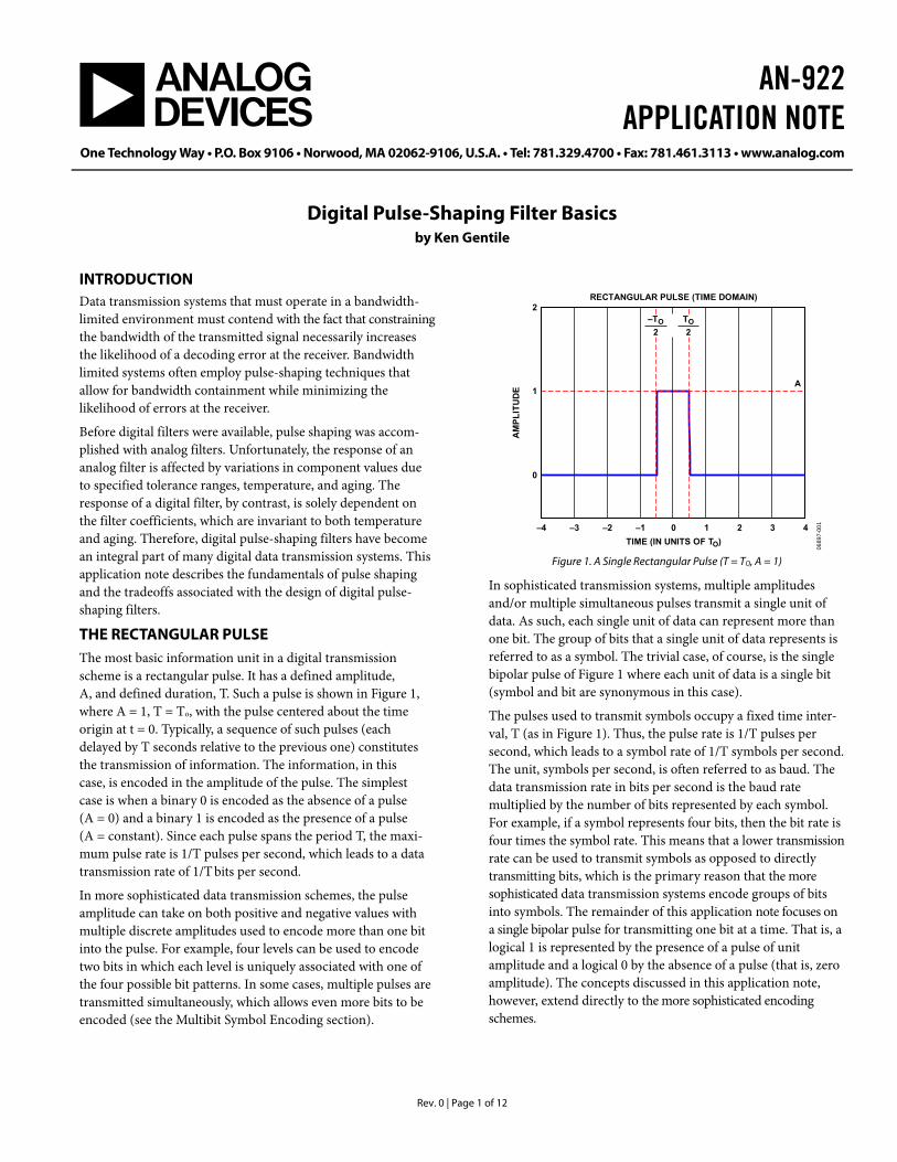
INTRODUCTION Data transmission systems that must operate in a bandwidth-limited environment must contend with the fact that constraining the bandwidth of the transmitted signal necessarily increases the likelihood of a decoding error at the receiver. Bandwidth limited systems often employ pulse-shaping techniques that allow for bandwidth containment while minimizing the likelihood of errors at the receiver.
Before digital filters were available, pulse shaping was accom-plished with analog filters. Unfortunately, the response of an analog filter is affected by variations in component values due to specified tolerance ranges, temperature, and aging. The response of a digital filter, by contrast, is solely dependent on the filter coefficients, which are invariant to both temperature and aging. Therefore, digital pulse-shaping filters have become an integral part of many digital data transmission systems. This application note describes the fundamentals of pulse shaping and the tradeoffs associated with the design of digital pulse-shaping filters.
THE RECTANGULAR PULSE The most basic information unit in a digital transmission scheme is a rectangular pulse. It has a defined amplitude, A, and defined duration, T. Such a pulse is shown in Figure 1, where A = 1, T = To, with the pulse centered about the time origin at t = 0. Typically, a sequence of such pulses (each delayed by T seconds relative to the previous one) constitutes the transmission of information. The information, in this case, is encoded in the amplitude of the pulse. The simplest case is when a binary 0 is encoded as the absence of a pulse (A = 0) and a binary 1 is encoded as the presence of a pulse (A = constant). Since each pulse spans the period T, the maxi-mum pulse rate is 1/T pulses per second, which leads to a data transmission rate of 1/T bits per second.
In more sophisticated data transmission schemes, the pulse amplitude can take on both positive and negative values with multiple discrete amplitudes used to encode more than one bit into the pulse. For example, four levels can be used to encode two bits in which each level is uniquely associated with one of the four possible bit patterns. In some cases, multiple pulses are transmitted simultaneously, which allows even more bits to be encoded (see the Multibit Symbol Encoding section).
–TO2
TO2
2
1
0
–4 –3 –2 –1 0 1 2 3 4A
MPL
ITU
DE
TIME (IN UNITS OF TO)
RECTANGULAR PULSE (TIME DOMAIN)
A
0689
7-00
1
Figure 1. A Single Rectangular Pulse (T = TO, A = 1)
In sophisticated transmission systems, multiple amplitudes and/or multiple simultaneous pulses transmit a single unit of data. As such, each single unit of data can represent more than one bit. The group of bits that a single unit of data represents is referred to as a symbol. The trivial case, of course, is the single bipolar pulse of Figure 1 where each unit of data is a single bit (symbol and bit are synonymous in this case).
The pulses used to transmit symbols occupy a fixed time inter-val, T (as in Figure 1). Thus, the pulse rate is 1/T pulses per second, which leads to a symbol rate of 1/T symbols per second. The unit, symbols per second, is often referred to as baud. The data transmission rate in bits per second is the baud rate multiplied by the number of bits represented by each symbol. For example, if a symbol represents four bits, then the bit rate is four times the symbol rate. This means that a lower transmission rate can be used to transmit symbols as opposed to directly transmitting bits, which is the primary reason that the more sophisticated data transmission systems encode groups of bits into symbols. The remainder of this application note focuses on a single bipolar pulse for transmitting one bit at a time. That is, a logical 1 is represented by the presence of a pulse of unit amplitude and a logical 0 by the absence of a pulse (that is, zero amplitude). The concepts discussed in this application note, however, extend directly to the more sophisticated encoding schemes.
AN-922
Rev. 0 | Page 2 of 12
TABLE OF CONTENTS Introduction ...................................................................................... 1 The Rectangular Pulse ..................................................................... 1 Spectrum of a Rectangular Pulse.................................................... 3 The Raised Cosine Filter.................................................................. 3 Pulse Shaping .................................................................................... 4 Digital Pulse-Shaping Filters........................................................... 5
Group 1 Plots: Error at the Edge of the Pass Band........................7 Group 2 Plots: Error at the Nyquist Frequency.............................8 Group 3 Plots: Minimum Stop Band Attenuation ........................9 Multibit Symbol Encoding ............................................................ 10 References........................................................................................ 11
AN-922
Rev. 0 | Page 3 of 12
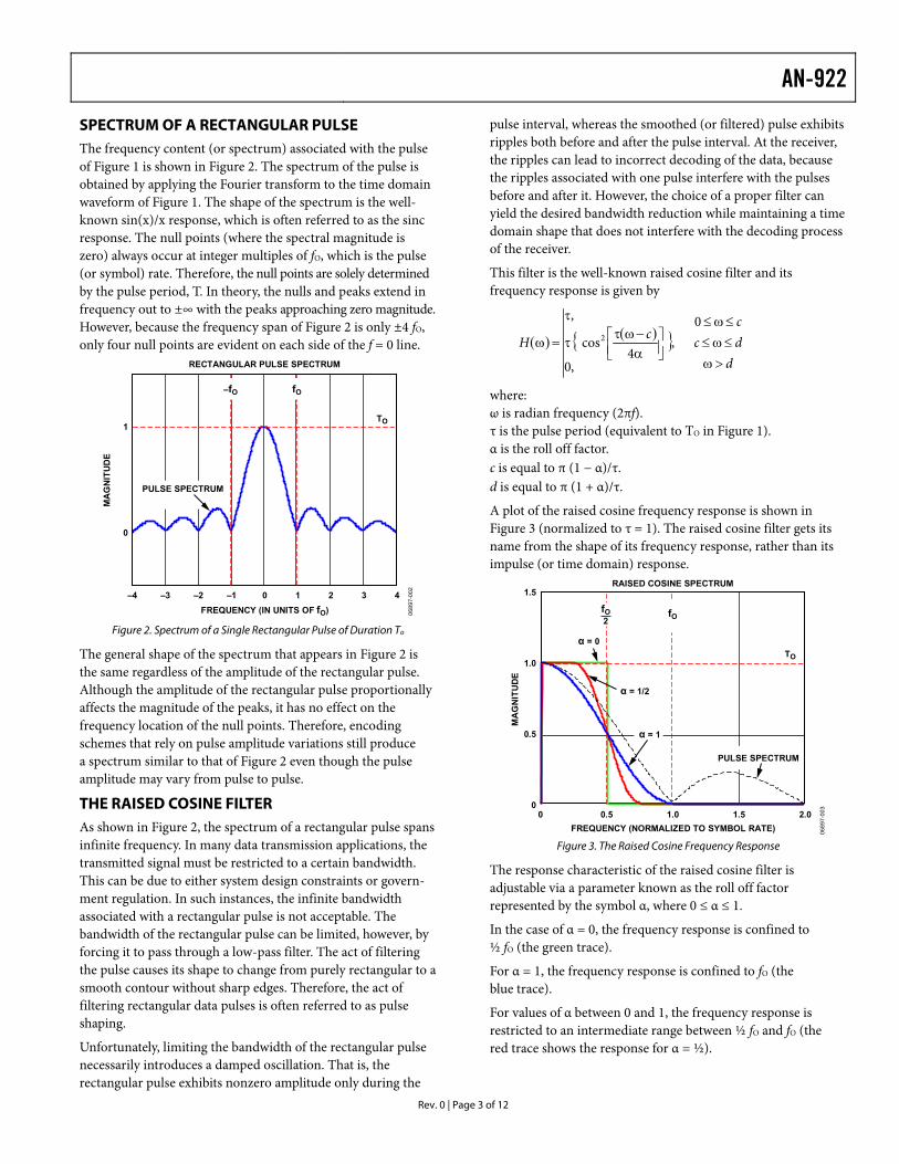
SPECTRUM OF A RECTANGULAR PULSE The frequency content (or spectrum) associated with the pulse of Figure 1 is shown in Figure 2. The spectrum of the pulse is obtained by applying the Fourier transform to the time domain waveform of Figure 1. The shape of the spectrum is the well-known sin(x)/x response, which is often referred to as the sinc response. The null points (where the spectral magnitude is zero) always occur at integer multiples of fO, which is the pulse (or symbol) rate. Therefore, the null points are solely determined by the pulse period, T. In theory, the nulls and peaks extend in frequency out to ±∞ with the peaks approaching zero magnitude. However, because the frequency span of Figure 2 is only ±4 fO, only four null points are evident on each side of the f = 0 line.
1
0
–4 –3 –2 –1 0 1 2 3 4
MA
GN
ITU
DE
FREQUENCY (IN UNITS OF fO)
RECTANGULAR PULSE SPECTRUM
TO
–fO fO
PULSE SPECTRUM
0689
7-00
2
Figure 2. Spectrum of a Single Rectangular Pulse of Duration To
The general shape of the spectrum that appears in Figure 2 is the same regardless of the amplitude of the rectangular pulse. Although the amplitude of the rectangular pulse proportionally affects the magnitude of the peaks, it has no effect on the frequency location of the null points. Therefore, encoding schemes that rely on pulse amplitude variations still produce a spectrum similar to that of Figure 2 even though the pulse amplitude may vary from pulse to pulse.
THE RAISED COSINE FILTER As shown in Figure 2, the spectrum of a rectangular pulse spans infinite frequency. In many data transmission applications, the transmitted signal must be restricted to a certain bandwidth. This can be due to either system design constraints or govern-ment regulation. In such instances, the infinite bandwidth associated with a rectangular pulse is not acceptable. The bandwidth of the rectangular pulse can be limited, however, by forcing it to pass through a low-pass filter. The act of filtering the pulse causes its shape to change from purely rectangular to a smooth contour without sharp edges. Therefore, the act of filtering rectangular data pulses is often referred to as pulse shaping.
Unfortunately, limiting the bandwidth of the rectangular pulse necessarily introduces a damped oscillation. That is, the rectangular pulse exhibits nonzero amplitude only during the
pulse interval, whereas the smoothed (or filtered) pulse exhibits ripples both before and after the pulse interval. At the receiver, the ripples can lead to incorrect decoding of the data, because the ripples associated with one pulse interfere with the pulses before and after it. However, the choice of a proper filter can yield the desired bandwidth reduction while maintaining a time domain shape that does not interfere with the decoding process of the receiver.
This filter is the well-known raised cosine filter and its frequency response is given by
( ) { ( ) }d
dcc
cH>ω
≤ω≤≤ω≤
⎥⎦⎤
⎢⎣⎡
α−ωτ
τ
τ
=ω0
,0
,4
cos
,2
where: ω is radian frequency (2πf). τ is the pulse period (equivalent to TO in Figure 1). α is the roll off factor. c is equal to π (1 − α)/τ. d is equal to π (1 + α)/τ.
A plot of the raised cosine frequency response is shown in Figure 3 (normalized to τ = 1). The raised cosine filter gets its name from the shape of its frequency response, rather than its impulse (or time domain) response.
1.0
0.5
1.5
00 0.5 1.51.0 2.0
MA
GN
ITU
DE
FREQUENCY (NORMALIZED TO SYMBOL RATE)
RAISED COSINE SPECTRUM
TO
fO
α = 0
α = 1
PULSE SPECTRUM
α = 1/2
fO2
0689
7-00
3
Figure 3. The Raised Cosine Frequency Response
The response characteristic of the raised cosine filter is adjustable via a parameter known as the roll off factor represented by the symbol α, where 0 ≤ α ≤ 1.
In the case of α = 0, the frequency response is confined to ½ fO (the green trace).
For α = 1, the frequency response is confined to fO (the blue trace).
For values of α between 0 and 1, the frequency response is restricted to an intermediate range between ½ fO and fO (the red trace shows the response for α = ½).
AN-922
Rev. 0 | Page 4 of 12
The dashed black trace is the spectrum of a rectangular pulse and is included for the sake of comparison.
There are three significant frequency points associated with the raised cosine response. The first is known as the Nyquist frequency, which occurs at ½ fO (that is, ½ the pulse rate). According to communication theory, this is the minimum possible bandwidth that can be used to transmit data without loss of information. Note that the raised cosine response crosses through the ½ amplitude point at ½ fo regardless of the value of α. The second significant frequency point is the stop band frequency (fSTOP) defined as the frequency at which the response first reaches zero magnitude. It is related to α by:
2)1( O
STOPf
f α+=
The third, and final, significant frequency point is the pass band frequency (fPASS) defined as the frequency at which the response first begins to depart from its peak magnitude. The raised cosine response is perfectly flat from f = 0 (DC) to fPASS, where:
2)1( O
PASSf
f α−=
Sometimes it is desirable to implement the raised cosine response as the product of two identical responses, one at the transmitter and the other at the receiver. In such cases, the response becomes a square-root raised cosine response since the product of the two responses yields the desired raised cosine response. The square-root raised cosine response is given below. Note that the variable definitions are the same as for the raised cosine response.
( ) { ( ) }d
dcc
cH>ω
≤ω≤≤ω≤
⎥⎦⎤
⎢⎣⎡
α−ωτ
τ
τ
=ω0
,0
,4
cos
,
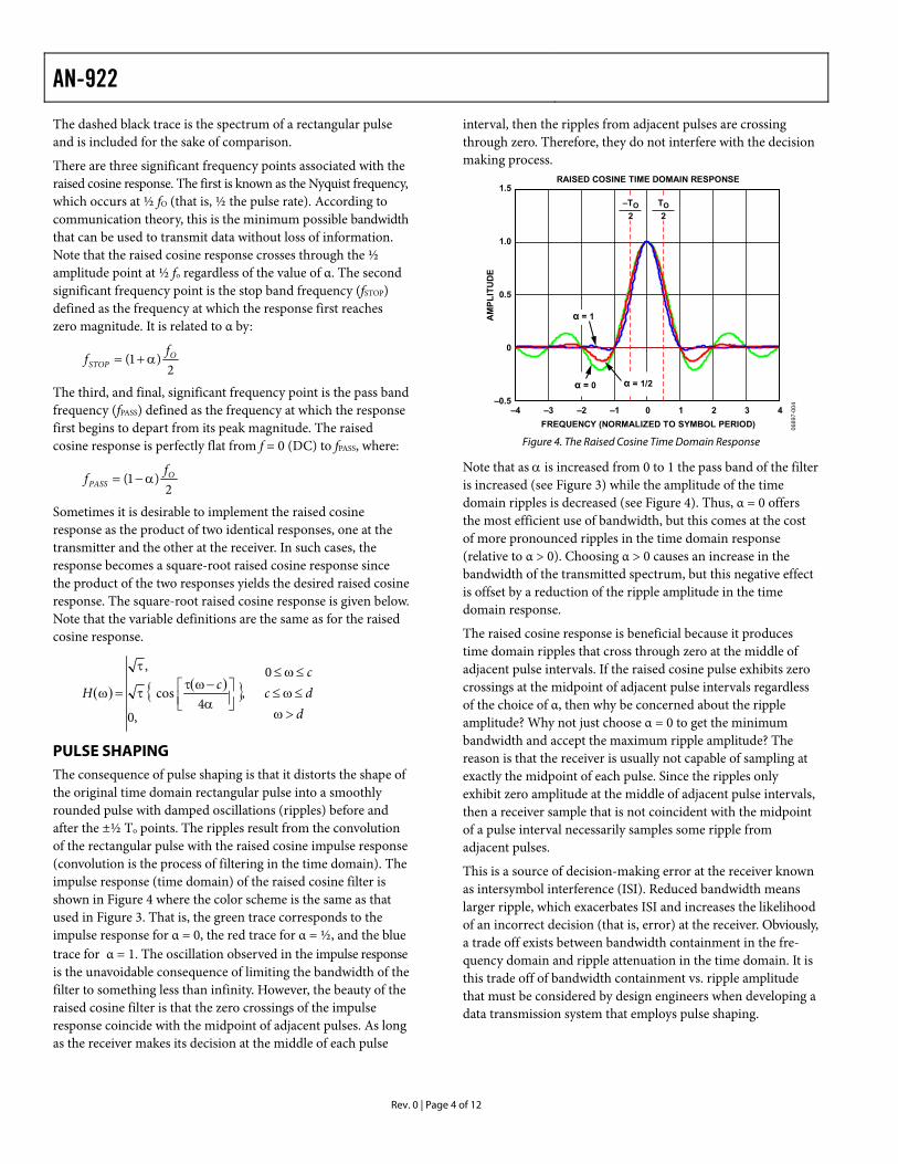
PULSE SHAPING The consequence of pulse shaping is that it distorts the shape of the original time domain rectangular pulse into a smoothly rounded pulse with damped oscillations (ripples) before and after the ±½ To points. The ripples result from the convolution of the rectangular pulse with the raised cosine impulse response (convolution is the process of filtering in the time domain). The impulse response (time domain) of the raised cosine filter is shown in Figure 4 where the color scheme is the same as that used in Figure 3. That is, the green trace corresponds to the impulse response for α = 0, the red trace for α = ½, and the blue trace for α = 1. The oscillation observed in the impulse response is the unavoidable consequence of limiting the bandwidth of the filter to something less than infinity. However, the beauty of the raised cosine filter is that the zero crossings of the impulse response coincide with the midpoint of adjacent pulses. As long as the receiver makes its decision at the middle of each pulse
interval, then the ripples from adjacent pulses are crossing through zero. Therefore, they do not interfere with the decision making process.
1.0
0.5
0
1.5
–0.5–4 –3 –2 –1 0 1 2 3 4
AM
PLIT
UD
E
FREQUENCY (NORMALIZED TO SYMBOL PERIOD)
RAISED COSINE TIME DOMAIN RESPONSE
–TO2
TO2
α = 0 α = 1/2
α = 1
0689
7-00
4
Figure 4. The Raised Cosine Time Domain Response
Note that as α is increased from 0 to 1 the pass band of the filter is increased (see Figure 3) while the amplitude of the time domain ripples is decreased (see Figure 4). Thus, α = 0 offers the most efficient use of bandwidth, but this comes at the cost of more pronounced ripples in the time domain response (relative to α > 0). Choosing α > 0 causes an increase in the bandwidth of the transmitted spectrum, but this negative effect is offset by a reduction of the ripple amplitude in the time domain response.
The raised cosine response is beneficial because it produces time domain ripples that cross through zero at the middle of adjacent pulse intervals. If the raised cosine pulse exhibits zero crossings at the midpoint of adjacent pulse intervals regardless of the choice of α, then why be concerned about the ripple amplitude? Why not just choose α = 0 to get the minimum bandwidth and accept the maximum ripple amplitude? The reason is that the receiver is usually not capable of sampling at exactly the midpoint of each pulse. Since the ripples only exhibit zero amplitude at the middle of adjacent pulse intervals, then a receiver sample that is not coincident with the midpoint of a pulse interval necessarily samples some ripple from adjacent pulses.
This is a source of decision-making error at the receiver known as intersymbol interference (ISI). Reduced bandwidth means larger ripple, which exacerbates ISI and increases the likelihood of an incorrect decision (that is, error) at the receiver. Obviously, a trade off exists between bandwidth containment in the fre-quency domain and ripple attenuation in the time domain. It is this trade off of bandwidth containment vs. ripple amplitude that must be considered by design engineers when developing a data transmission system that employs pulse shaping.
AN-922
Rev. 0 | Page 5 of 12
DIGITAL PULSE-SHAPING FILTERS Raised cosine filters are frequently implemented as digital rather than analog filters. A digital implementation means that the filter is subject to the constraints of a Nyquist system. That is, the filter sample rate must be twice that of the input band-width in order to avoid aliasing. If a digital pulse shaping filter operates at a sample rate of fO (the symbol rate), then the maximum input bandwidth must be limited to ½ fO. This poses a problem because Figure 3 shows that the required bandwidth is greater than ½ fO for α > 0 and can extend to fo for α = 1. The implication is that digital pulse-shaping filters must oversample the symbol pulses by at least a factor of two in order to accommodate bandwidths as high as fO.
Although digital filters typically produce a desired frequency domain response, they actually perform the filtering task in the time domain. That is, the digital filter coefficients (taps) define the impulse response of the filter (a time domain characteristic), which produces the desired frequency response. Therefore, the digital filter design task is greatly simplified with knowledge of the desired impulse response rather than the frequency response. To this end, the impulse response of the raised cosine filter is given in the following equation.
( )
⎟⎟⎟⎟⎟
⎠
⎞
⎜⎜⎜⎜⎜
⎝
⎛
⎟⎠⎞
⎜⎝⎛
τα
−
⎟⎠⎞
⎜⎝⎛
τπα
×
⎟⎟⎟⎟
⎠
⎞
⎜⎜⎜⎜
⎝
⎛
⎟⎠⎞
⎜⎝⎛
τπ
⎟⎠⎞
⎜⎝⎛
τπ
= 221
cossin
t
t
t
t
th
The variable definitions are the same as for the raised cosine frequency response, except that the time variable, t, replaces the frequency variable, ω. Although h(t) is indeterminate for t = 0 and undefined for t = ±τ/(2α), it can be shown that:
( ) 10 =h
and
⎟⎠⎞
⎜⎝⎛
απα
=⎟⎠⎞
⎜⎝⎛
ατ
±2
sin22
h
Likewise, the impulse response of the square-root raised cosine filter is given by
( )
( ) ( )
⎥⎥⎥⎥
⎦
⎤
⎢⎢⎢⎢
⎣
⎡
⎟⎠⎞
⎜⎝⎛
τα
−
⎟⎠⎞
⎜⎝⎛
τα−π
ατ
+⎟⎠⎞
⎜⎝⎛
τα+π
⎟⎟⎠
⎞⎜⎜⎝
⎛τπ
α= 241
1sin4
1cos4
t
tt
t
th
Again, h(t) is undefined at t = 0, but it can be shown that
( ) ⎥⎦⎤
⎢⎣⎡
⎟⎠⎞
⎜⎝⎛ −
πα+⎟⎟
⎠
⎞⎜⎜⎝
⎛τ
= 14110h
It turns out that h(t) is also undefined at t = ± τ/(4α), but without remedy. Therefore, avoid designing a square-root raised cosine filter with any taps that coincide with this value of t.
Generally, digital pulse-shaping filters are implemented as finite impulse response (FIR) filters rather than as infinite impulse response (IIR) filters for several reasons.
• FIR filters can be easily designed with linear phase response, which can be of paramount importance in applications that must guarantee constant group delay.
• FIR filters do not suffer from limit cycles, which often plague IIR designs. Limit cycles are small oscillations that persist at the output of the filter even when the input signal is removed.
• FIR filters are intrinsically stable because they do not incorporate feedback. The IIR architecture, on the other hand, does have feedback so the choice of coefficients has an impact on stability. In fact, an IIR filter can oscillate if care is not taken to ensure an unconditionally stable design.
• If the filter is implemented in hardware (as opposed to software), FIR filters lend themselves to a polyphase architecture, which significantly reduces the amount of hardware required. This is important because an IIR filter generally requires fewer filter coefficients (or taps) than an FIR filter with a similar frequency response characteristic. Since the amount of hardware required to implement the filter is directly proportional to the number of taps, FIR filters tend to be more hardware intensive. However, the hardware reduction offered by the polyphase option tends to make the IIR hardware advantage less significant.
For the sake of brevity, only the FIR implementation is considered in this application note. However, regardless of whether one chooses a FIR or IIR digital filter implementation, the filter response is, at best, an approximation of the ideal response (raised cosine in this case). The degree to which the filter response matches the ideal response is dependent on two parameters: the amount of over sampling (M) and the number of taps (N).
Generally, N is chosen to be an integer multiple of M when designing a FIR for the purpose of pulse shaping. This guaran-tees that the impulse response of the filter spans an integer number of pulses. As such, the number of filter taps is given by
N = D × M
where D and M are both integers.
The filter order is odd or even based on whether N is odd or even. If a particular filter order is preferred, then it is customary to add 1 to N to yield the desired order. Note that the value of D defines the number of symbols spanned by the impulse response of the filter. Generally, a larger D means a better approximation of the ideal response. Unfortunately, the complexity of the filter is proportional to D, so it is advantageous to use the smallest value of D that meets the filtering requirements. Determination of the smallest acceptable value of D can be a daunting task, especially if the filter must be designed to handle a wide range of α values. This is because the frequency response of the filter
AN-922
Rev. 0 | Page 6 of 12
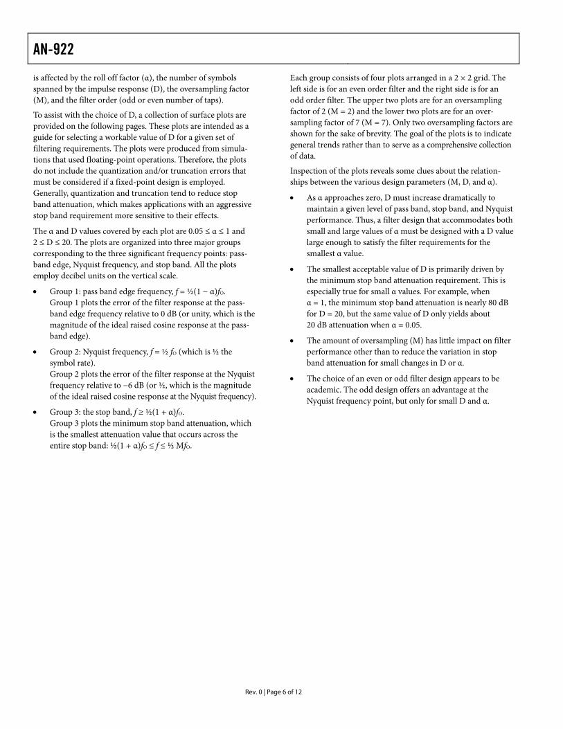
is affected by the roll off factor (α), the number of symbols spanned by the impulse response (D), the oversampling factor (M), and the filter order (odd or even number of taps).
To assist with the choice of D, a collection of surface plots are provided on the following pages. These plots are intended as a guide for selecting a workable value of D for a given set of filtering requirements. The plots were produced from simula-tions that used floating-point operations. Therefore, the plots do not include the quantization and/or truncation errors that must be considered if a fixed-point design is employed. Generally, quantization and truncation tend to reduce stop band attenuation, which makes applications with an aggressive stop band requirement more sensitive to their effects.
The α and D values covered by each plot are 0.05 ≤ α ≤ 1 and 2 ≤ D ≤ 20. The plots are organized into three major groups corresponding to the three significant frequency points: pass-band edge, Nyquist frequency, and stop band. All the plots employ decibel units on the vertical scale.
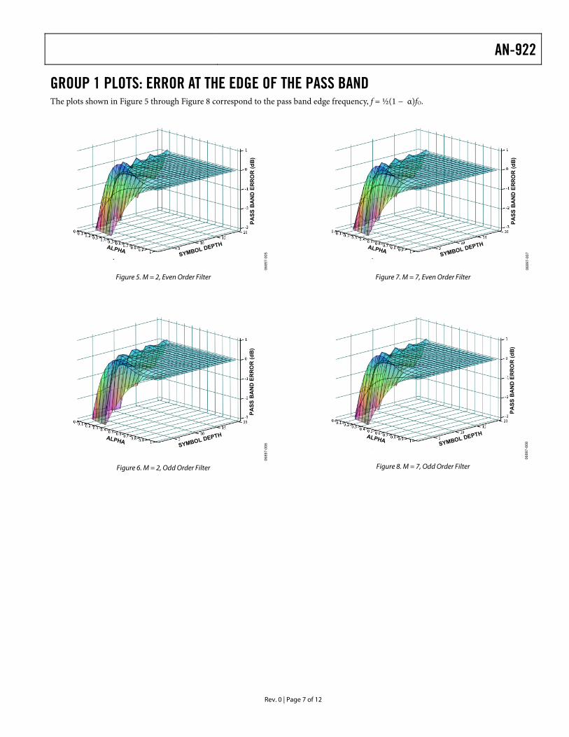
• Group 1: pass band edge frequency, f = ½(1 − α)fO.
Group 1 plots the error of the filter response at the pass-band edge frequency relative to 0 dB (or unity, which is the magnitude of the ideal raised cosine response at the pass-band edge).
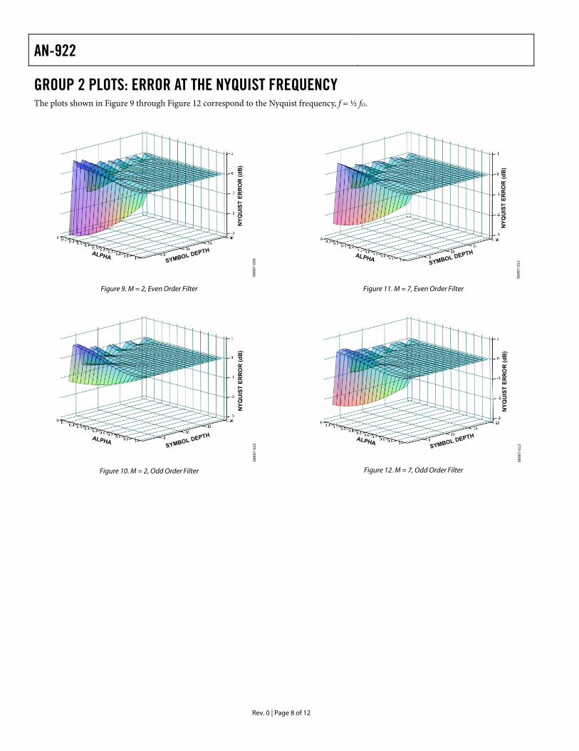
• Group 2: Nyquist frequency, f = ½ fO (which is ½ the symbol rate). Group 2 plots the error of the filter response at the Nyquist frequency relative to −6 dB (or ½, which is the magnitude of the ideal raised cosine response at the Nyquist frequency).
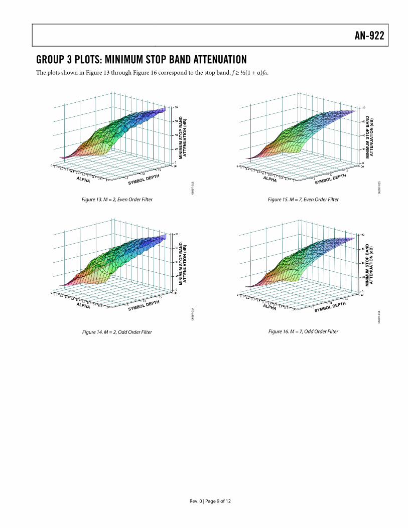
• Group 3: the stop band, f ≥ ½(1 + α)fO. Group 3 plots the minimum stop band attenuation, which is the smallest attenuation value that occurs across the entire stop band: ½(1 + α)fO ≤ f ≤ ½ MfO.
Each group consists of four plots arranged in a 2 × 2 grid. The left side is for an even order filter and the right side is for an odd order filter. The upper two plots are for an oversampling factor of 2 (M = 2) and the lower two plots are for an over-sampling factor of 7 (M = 7). Only two oversampling factors are shown for the sake of brevity. The goal of the plots is to indicate general trends rather than to serve as a comprehensive collection of data.
Inspection of the plots reveals some clues about the relation-ships between the various design parameters (M, D, and α).
• As α approaches zero, D must increase dramatically to maintain a given level of pass band, stop band, and Nyquist performance. Thus, a filter design that accommodates both small and large values of α must be designed with a D value large enough to satisfy the filter requirements for the smallest α value.
• The smallest acceptable value of D is primarily driven by the minimum stop band attenuation requirement. This is especially true for small α values. For example, when α = 1, the minimum stop band attenuation is nearly 80 dB for D = 20, but the same value of D only yields about 20 dB attenuation when α = 0.05.
• The amount of oversampling (M) has little impact on filter performance other than to reduce the variation in stop band attenuation for small changes in D or α.
• The choice of an even or odd filter design appears to be academic. The odd design offers an advantage at the Nyquist frequency point, but only for small D and α.
AN-922
Rev. 0 | Page 7 of 12
GROUP 1 PLOTS: ERROR AT THE EDGE OF THE PASS BAND The plots shown in Figure 5 through Figure 8 correspond to the pass band edge frequency, f = ½(1 − α)fO.
SYMBOL DEPTHALPHAPA
SS B
AN
D E
RR
OR
(dB
)
0689
7-00
5
Figure 5. M = 2, Even Order Filter
SYMBOL DEPTHALPHA
PASS
BA
ND
ER
RO
R (d
B)
0689
7-00
6
Figure 6. M = 2, Odd Order Filter
SYMBOL DEPTHALPHA
PASS
BA
ND
ER
RO
R (d
B)
0689
7-00
7
Figure 7. M = 7, Even Order Filter
SYMBOL DEPTHALPHA
PASS
BA
ND
ER
RO
R (d
B)
0689
7-00
8
Figure 8. M = 7, Odd Order Filter
AN-922
Rev. 0 | Page 8 of 12
GROUP 2 PLOTS: ERROR AT THE NYQUIST FREQUENCY The plots shown in Figure 9 through Figure 12 correspond to the Nyquist frequency, f = ½ fO.
SYMBOL DEPTHALPHA
NYQ
UIS
T ER
RO
R (d
B)
0689
7-00
9
Figure 9. M = 2, Even Order Filter
SYMBOL DEPTHALPHA
NYQ
UIS
T ER
RO
R (d
B)
0689
7-01
0
Figure 10. M = 2, Odd Order Filter
SYMBOL DEPTHALPHA
NYQ
UIS
T ER
RO
R (d
B)
0689
7-01
1
Figure 11. M = 7, Even Order Filter
SYMBOL DEPTHALPHA
NYQ
UIS
T ER
RO
R (d
B)
0689
7-01
2
Figure 12. M = 7, Odd Order Filter
AN-922
Rev. 0 | Page 9 of 12
GROUP 3 PLOTS: MINIMUM STOP BAND ATTENUATION The plots shown in Figure 13 through Figure 16 correspond to the stop band, f ≥ ½(1 + α)fO.
SYMBOL DEPTHALPHAM
INIM
UM
STO
P B
AN
DA
TTEN
UA
TIO
N (d
B)
0689
7-01
3
Figure 13. M = 2, Even Order Filter
SYMBOL DEPTHALPHA
MIN
IMU
M S
TOP
BA
ND
ATT
ENU
ATI
ON
(dB
)
0689
7-01
4
Figure 14. M = 2, Odd Order Filter
SYMBOL DEPTHALPHA
MIN
IMU
M S
TOP
BA
ND
ATT
ENU
ATI
ON
(dB
)
0689
7-01
5
Figure 15. M = 7, Even Order Filter
SYMBOL DEPTHALPHA
MIN
IMU
M S
TOP
BA
ND
ATT
ENU
ATI
ON
(dB
)
0689
7-01
6
Figure 16. M = 7, Odd Order Filter
AN-922
Rev. 0 | Page 10 of 12
MULTIBIT SYMBOL ENCODING
A commonly used multibit pulse-encoding scheme is quad-rature amplitude modulation (QAM). QAM relies on two mechanisms to encode bits. One is the pulse amplitude, which can assume both positive and negative values, and the other is the use of two simultaneous pulses. The latter requires two independent baseband channels, one for each pulse. One channel is referred to as the I, or in-phase, channel and the other as the Q, or quadrature, channel.
QAM comes in a variety of forms depending on the number of bits encoded into each pair of pulses. For example, 16 QAM uses a 4-bit symbol to represent 16 possible symbol values; 64 QAM uses a 6-bit symbol to represent 64 possible symbol values; and 256 QAM uses an 8-bit symbol to represent 256 possible symbol values. Generally, QAM symbols encode an even number of bits (4, 6, 8 and so on), but odd bit schemes, though uncommon, exist as well.
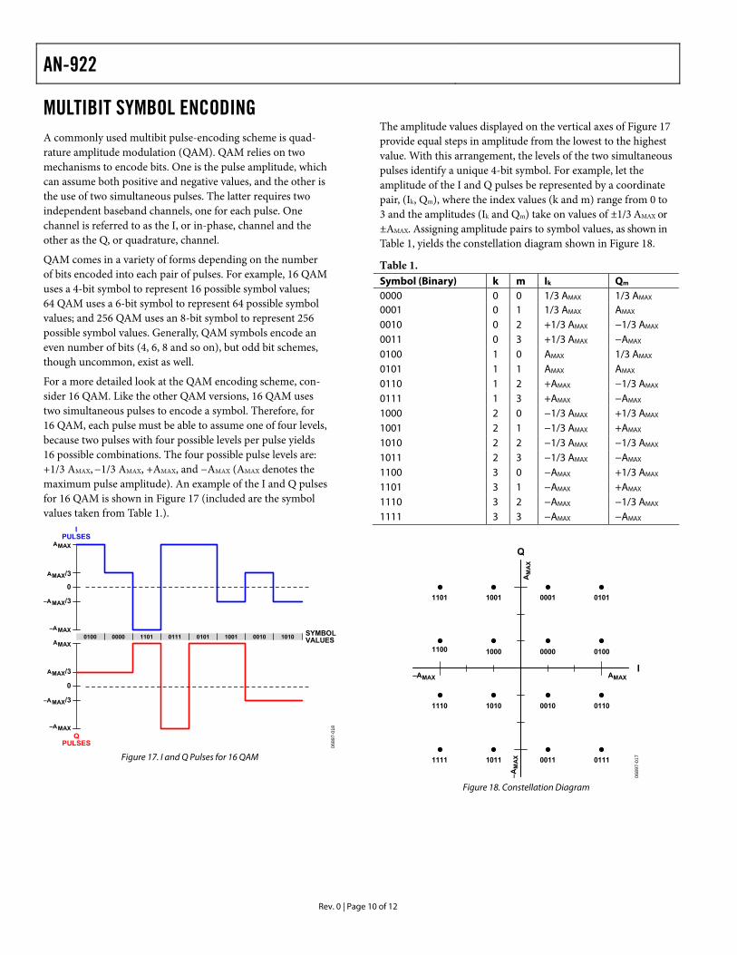
For a more detailed look at the QAM encoding scheme, con-sider 16 QAM. Like the other QAM versions, 16 QAM uses two simultaneous pulses to encode a symbol. Therefore, for 16 QAM, each pulse must be able to assume one of four levels, because two pulses with four possible levels per pulse yields 16 possible combinations. The four possible pulse levels are: +1/3 AMAX, −1/3 AMAX, +AMAX, and −AMAX (AMAX denotes the maximum pulse amplitude). An example of the I and Q pulses for 16 QAM is shown in Figure 17 (included are the symbol values taken from Table 1.).
0689
7-01
8
0
IPULSES
0
–AMAX
–AMAX/3
–AMAX/3
AMAX/3
AMAX/3
AMAX
AMAX
–AMAX
QPULSES
0100 1010001010010101011111010000 SYMBOLVALUES
Figure 17. I and Q Pulses for 16 QAM
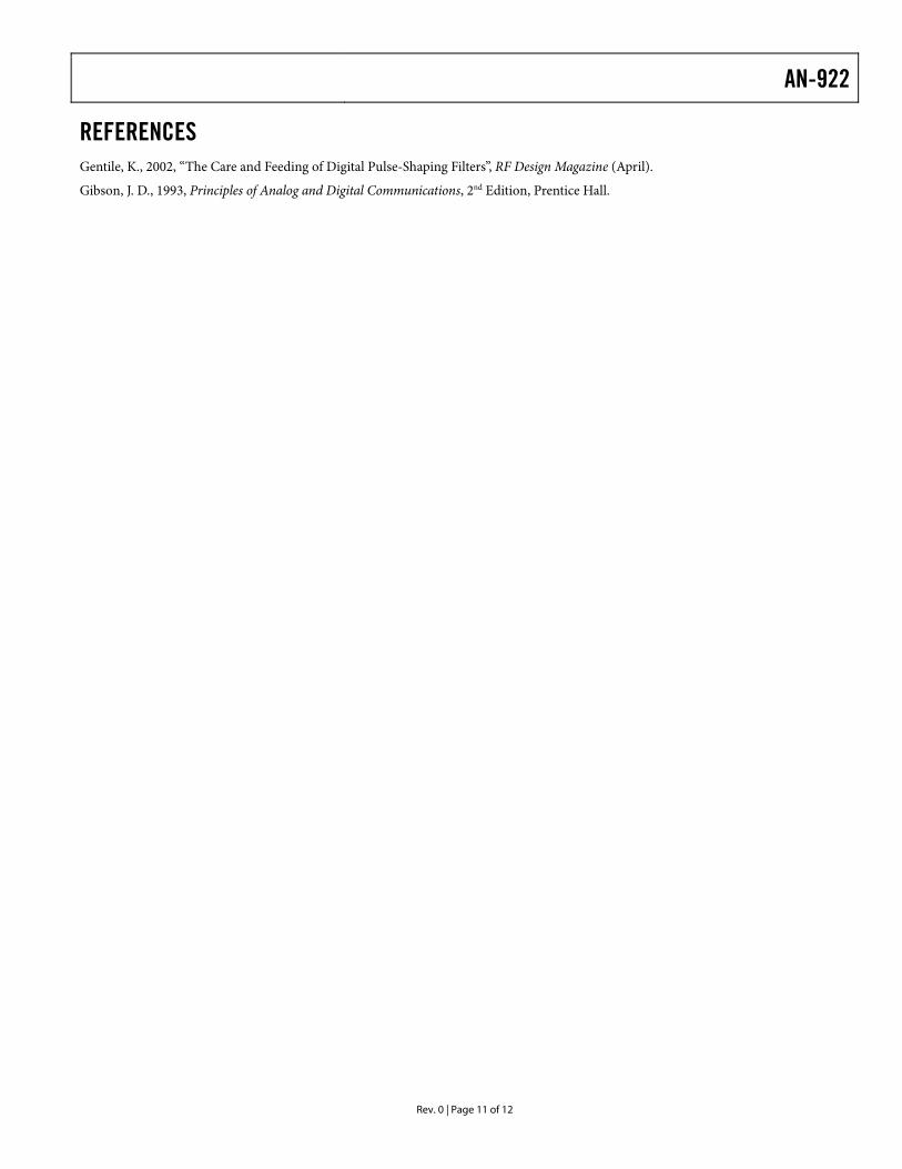
The amplitude values displayed on the vertical axes of Figure 17 provide equal steps in amplitude from the lowest to the highest value. With this arrangement, the levels of the two simultaneous pulses identify a unique 4-bit symbol. For example, let the amplitude of the I and Q pulses be represented by a coordinate pair, (Ik, Qm), where the index values (k and m) range from 0 to 3 and the amplitudes (Ik and Qm) take on values of ±1/3 AMAX or ±AMAX. Assigning amplitude pairs to symbol values, as shown in Table 1, yields the constellation diagram shown in Figure 18.
Table 1. Symbol (Binary) k m Ik Qm 0000 0 0 1/3 AMAX 1/3 AMAX 0001 0 1 1/3 AMAX AMAX 0010 0 2 +1/3 AMAX −1/3 AMAX 0011 0 3 +1/3 AMAX −AMAX 0100 1 0 AMAX 1/3 AMAX 0101 1 1 AMAX AMAX 0110 1 2 +AMAX −1/3 AMAX 0111 1 3 +AMAX −AMAX 1000 2 0 −1/3 AMAX +1/3 AMAX 1001 2 1 −1/3 AMAX +AMAX 1010 2 2 −1/3 AMAX −1/3 AMAX 1011 2 3 −1/3 AMAX −AMAX 1100 3 0 −AMAX +1/3 AMAX 1101 3 1 −AMAX +AMAX 1110 3 2 −AMAX −1/3 AMAX 1111 3 3 −AMAX −AMAX
0689
7-01
7
I
Q
AMAX–AMAX
AM
AX
–AM
AX
0000
0111
0110
0101
0100
0011
0010
0001
1000
1111
1110
1101
1100
1011
1010
1001
Figure 18. Constellation Diagram
AN-922
Rev. 0 | Page 11 of 12
REFERENCES Gentile, K., 2002, “The Care and Feeding of Digital Pulse-Shaping Filters”, RF Design Magazine (April).
Gibson, J. D., 1993, Principles of Analog and Digital Communications, 2nd Edition, Prentice Hall.

AN-922
Rev. 0 | Page 12 of 12
NOTES
©2007 Analog Devices, Inc. All rights reserved. Trademarks and registered trademarks are the property of their respective owners. AN06897-0-9/07(0)