ONE-SIDED WEIGHTED APPROXIMATION

ONE-SIDED WEIGHTED APPROXIMATION

by

Oleksandr Maizlish

A Thesis submitted to the Faculty of Graduate Studies of

The University of Manitoba

in partial fulfilment of the requirements of the degree of

MASTER OF SCIENCE

Department of Mathematics

University of Manitoba

Winnipeg

Copyright c© 2008 by Oleksandr Maizlish

UNIVERSITY OF MANITOBA

DEPARTMENT OF MATHEMATICS

The undersigned hereby certify that they have read and

recommend to the Faculty of Graduate Studies for acceptance a thesis

entitled “One-sided weighted approximation” by Oleksandr Maizlish in

partial fulfillment of the requirements for the degree of Master of Science.

Dated:

Research Supervisor:K. A. Kopotun

Examining Committee:N. Zorboska

Examining Committee:X. Wang

ii

UNIVERSITY OF MANITOBA

Date: August 2008

Author: Oleksandr Maizlish

Title: One-sided weighted approximation

Department: Mathematics

Degree: M.Sc.

Convocation: October

Year: 2008

Permission is herewith granted to University of Manitoba to circulateand to have copied for non-commercial purposes, at its discretion, the abovetitle upon the request of individuals or institutions.

Signature of Author

THE AUTHOR RESERVES OTHER PUBLICATION RIGHTS, ANDNEITHER THE THESIS NOR EXTENSIVE EXTRACTS FROM IT MAYBE PRINTED OR OTHERWISE REPRODUCED WITHOUT THE AUTHOR’SWRITTEN PERMISSION.

THE AUTHOR ATTESTS THAT PERMISSION HAS BEEN OBTAINEDFOR THE USE OF ANY COPYRIGHTED MATERIAL APPEARING IN THISTHESIS (OTHER THAN BRIEF EXCERPTS REQUIRING ONLY PROPERACKNOWLEDGEMENT IN SCHOLARLY WRITING) AND THAT ALL SUCHUSE IS CLEARLY ACKNOWLEDGED.

iii

Abstract

This thesis is devoted to weighted approximation by polynomials on the real line

and deals with what is called one-sided weighted approximation in Approximation

Theory. More precisely, we investigate the existence of a sequence of polynomials

which lie above (or below) a given function and approximate it arbitrarily well.

We present an overview of this subject in the Lp-spaces, starting with the early

works of Freud and ending by the latest results in this area. This branch of weighted

approximation was developed in the last 30-40 years and now contains a big variety of

techniques and approaches. We develop new methods on one-sided approximation in

the L∞-norm and obtain several results. We also discuss a number of open questions

and describe possible directions of future research in this area.

iv

Acknowledgments

The author would like to express his gratitude and profound respect to

Dr. Kirill Kopotun and Dr. Andriy Prymak

for their numerous suggestions.

v

Contents

1 Introduction 1

1.1 Some history of Polynomial Approximation . . . . . . . . . . . . . . . 1

1.2 Preliminaries . . . . . . . . . . . . . . . . . . . . . . . . . . . . . . . 2

1.3 Weighted Approximation on the Real Line . . . . . . . . . . . . . . . 3

2 Weighted unconstrained polynomial approximation on the real line 9

2.1 Rate of approximation . . . . . . . . . . . . . . . . . . . . . . . . . . 9

2.1.1 Notations and Definitions . . . . . . . . . . . . . . . . . . . . 9

2.1.2 Jackson-Favard inequality . . . . . . . . . . . . . . . . . . . . 10

2.1.3 Jackson Theorem . . . . . . . . . . . . . . . . . . . . . . . . . 13

2.2 Restricted Range Inequalities . . . . . . . . . . . . . . . . . . . . . . 16

3 One-Sided Lp Methods 19

3.1 Freud and Nevai’s One-sided L1 method . . . . . . . . . . . . . . . . 19

3.2 Partially one-sided polynomial approximation on the real line and its

applications . . . . . . . . . . . . . . . . . . . . . . . . . . . . . . . . 24

3.2.1 Estimates for certain classes of functions . . . . . . . . . . . . 25

3.2.2 Applications . . . . . . . . . . . . . . . . . . . . . . . . . . . . 26

4 One-Sided L∞ Weighted Approximation 28

5 Conclusions 34

Bibliography 35

vi

Chapter 1

Introduction

1.1 Some history of Polynomial Approximation

Back in the 19-th century during the early industrial revolution, physics, chemistry

and other natural sciences required a development of a new tool in order to construct

new mechanisms, more precise and efficient. Inventions like Watt’s idea of parallel

motion and designing of electric filter networks were supported by new mathemat-

ical observations and methods of approximation (in particular, polynomial approx-

imation). Great contributions were made by the famous Russian mathematicians

Chebyshev and Markov.

At the same time, classical mathematics already investigated the existence of a

continuous nowhere differentiable function, which generated a lot of interest in the

whole mathematical community. Bolzano was the first to construct such a func-

tion. Continuous nowhere differentiable functions might seem to some as pathologi-

cal. This accentuated and intensified the need for analytic approximation of certain

classes of functions. As a result, this led to a fundamental theorem of Approxima-

tion Theory, which was discovered in 1885 by Weierstrass [32], one of the greatest

people in mathematics. Namely, Weierstrass proved that any continuous function

on an interval can be approximated by algebraic polynomials as well as desired,

hence establishing what we now know as the density of polynomials (in the space of

all continuous functions on an interval). Various proofs of the Weierstrass theorem

1

Chapter 1: Introduction 2

were presented by Weierstrass, Picard, Fejer, Landau, de la Valle Poussin, Runge,

Lebesgue, Mittag-Leffler, Lerch, Volterra. The last of the early proofs was due to

Bernstein [4] who is well known by his works on Probability Theory, Constructive

function theory, mathematical foundations of genetics, etc. This proof is quite dif-

ferent from the previous proofs, and has had a profound impact in various areas. In

[4], Bernstein introduced what we today call Bernstein polynomials.

As any great theorem, the Weierstrass Theorem was significant in its influence

on the development of several mathematical areas, one of them being the field of

Approximation Theory. It led to many interesting generalizations such as the Stone-

Weierstrass theorem, the Muntz theorem, the Bohman-Korovkin theorem, which

deal with the density of a given subset in the space of all continuous functions. In

particular, this thesis is devoted to a certain extension of the approximation on an

interval, namely, here we consider weighted approximation on the whole real line.

Finally, we mention that currently many modern directions in pure and applied

mathematics use the methods of approximation. Among them are Numerical analy-

sis, PDE, Learning theory, Geodesy, and more.

1.2 Preliminaries

In this section, we introduce some basic definitions and notations. For more details

and references see, for example, [1, 8].

• By C(S) we denote the set of all continuous functions on S. In particular,

C[a, b] is the space of all continuous functions f on [a, b], equipped with the

norm

‖f‖C[a,b] := maxx∈[a,b]

|f(x)|.

• Let (Ω, µ) be a measure space. By Lp(Ω) we denote the space of all measurable

functions f : Ω→ R such that

‖f‖Lp(Ω) :=

(∫Ω

|f(x)|pdµ(x)

)1/p

<∞.


Everywhere below, we assume that 1 ≤ p ≤ ∞ unless specifically stated oth-

erwise.

• Πn is the set of all algebraic polynomials of degree ≤ n.

• Let (X, ‖ · ‖X) be a (quasi) normed space, and Y ⊂ X be a subspace of X.

The number

EY (f)X := infy∈Y‖f − y‖X

is called the value of best approximation of the element f ∈ X by the subspace

Y . In particular, the value of best approximation of f ∈ C[a, b] by polynomials

of degree ≤ n is

En(f)C[a,b] := EΠn(f)C[a,b] = infP∈Πn

‖f − P‖C[a,b].

An element y∗ ∈ Y is called an element of best approximation of f ∈ X by the

subspace Y , if

EY (f)X = ‖f − y∗‖X .

If X is a Banach space and Y is a finite dimensional subspace of X, then, by

Borel’s Theorem [5] for any f ∈ X, there exists an element of best approxima-

tion of f by the subspace Y .

Let Z be a subset (usually, a cone) of X (for example, Z can be the set of all

monotone polynomials on [a, b]). Then

En(f, Z)X = infy∈Z∩Πn

‖f − y‖X

is the error of approximation of f by polynomials restricted to Z.

• A function f ∈ C(R) is said to be of polynomial growth (at ∞) if there exist a

polynomial P and a constant L > 0 such that |f(x)| ≤ L|P (x)|, for all x ∈ R.

1.3 Weighted Approximation on the Real Line

The origins of weighted approximation come from the manuscript [3] by Bernstein,

where the problem that is now known as Bernstein’s Approximation Problem was

posed.


For a continuous W : R → (0, 1], denote by CW := CW (R) the space of all

continuous functions f : R → R such that limx→±∞

f(x)W (x) = 0, equipped with

the norm ‖f‖W := ‖f‖CW := supx∈R |f(x)W (x)|. We call W a weight function.

Bernstein’s Approximation Problem is stated as follows:

Problem 1.1 (Bernstein’s Approximation Problem). Characterize all weights W

such that, for every f ∈ CW , there exists a sequence of polynomials Pn∞n=0 such

that

limn→∞

‖f − Pn‖W = 0?

In other words, Bernstein’s approximation problem asks for a description of the

class of all weight functions W such that polynomials are dense in CW . This problem

was solved independently by Achieser, Mergelyan, and Pollard in 1950’s (see, e.g.,

[20]).

Recall that a subset of the normed space is called fundamental if the closure of

its linear span is the whole space. The following theorem was presented by Pollard

[28]:

Theorem 1.2 (Solution of Bernstein’s Approximation Problem). Suppose that, for

all n ∈ N, xn ∈ CW . Then in order that xn∞n=0 be fundamental in CW it is necessary

and sufficient that

(i)

+∞∫−∞

log(1/W (t))

1 + t2dt =∞;

and

(ii) there exists a sequence of polynomials Pn∞n=1 such that, for each x,

limn→∞

Pn(x)W (x) = 1 while supn≥1‖Pn‖W <∞.

Since polynomials are unbounded at infinity, it is natural to require W to decay

sufficiently fast at infinity in order to counterweight the growth of every polynomial.

The so-called Freud’s weights Wα(x) = e−|x|α, which are of particular interest in this

thesis, satisfy both conditions (i) and (ii) iff α ≥ 1, and therefore the linear span of


xn, n ∈ N, is dense in CWα iff α ≥ 1. More recent results regarding approximation

with the exponential weights are discussed in s the survey [22] by Lubinsky. Some

important facts on this subject are also mentioned in Chapter 2.

The main goal of this thesis is to investigate a special kind of weighted ap-

proximation, the so-called one-sided weighted approximation. One-sided polynomial

approximation deals with the question on how well one can approximate a given

function by polynomials which lie above (or below) it. Results regarding one-sided

approximation on an interval in various functional spaces are presented in [2, 7, 18].

Below, we discuss a classical unweighted (uniform) approximation on an interval

[a, b] by algebraic polynomials. The rate of one-sided approximation in that case is

equivalent to the rate of the unconstrained approximation. Here is a short proof why

this is true. Let f ∈ C[a, b]. For a fixed n, let Pn be a polynomial of best approx-

imation among all polynomials of degree ≤ n. Weierstrass’s theorem implies that

limn→∞

‖f −Pn‖C[a,b] = 0. For any n ≥ 0, define polynomials Qn := Pn+‖f −Pn‖C[a,b].

Then, the polynomials Qn lie above the function f . Indeed, for all x ∈ [a, b],

Qn(x)− f(x) = Pn(x) + ‖f − Pn‖C[a,b] − f(x) ≥ ‖f − Pn‖C[a,b] − |f(x)− Pn(x)| ≥ 0,

and the error of the one-sided approximation

‖Qn − f‖C[a,b] ≤ ‖Qn − Pn‖C[a,b] + ‖Pn − f‖C[a,b] = 2‖f − Pn‖C[a,b] = 2En(f)C[a,b]

converges to 0 as fast as En(f)C[a,b]. Hence, one constructs one-sided approximation

on an interval by sufficiently lifting Pn.

This approach fails in the case of approximation in the Lp-spaces over a finite

interval, for p <∞. It is impossible to get an upper estimate on the rate of the one-

sided approximation on [−1, 1] even in terms of ‖f‖Lp[−1,1], since for the function

f such that f(x) = 0, x 6= 0, f(0) = 1, its Lp-norm is 0, and according to [17],

infn∈N∪0

infP≥f,P∈Πn

‖P − f‖Lp[−1,1] > 0. Though some kinds of estimates could still be

obtained (see, e.g., [17, 18]).

If one tries to generalize the problem of one-sided approximation to the real line,

the following question arises:


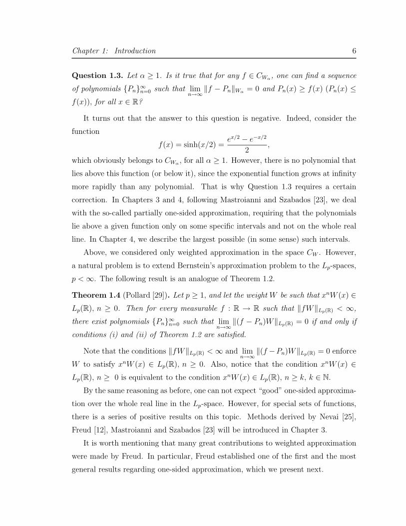
Question 1.3. Let α ≥ 1. Is it true that for any f ∈ CWα, one can find a sequence

of polynomials Pn∞n=0 such that limn→∞

‖f − Pn‖Wα = 0 and Pn(x) ≥ f(x) (Pn(x) ≤f(x)), for all x ∈ R?

It turns out that the answer to this question is negative. Indeed, consider the

function

f(x) = sinh(x/2) =ex/2 − e−x/2

2,

which obviously belongs to CWα , for all α ≥ 1. However, there is no polynomial that

lies above this function (or below it), since the exponential function grows at infinity

more rapidly than any polynomial. That is why Question 1.3 requires a certain

correction. In Chapters 3 and 4, following Mastroianni and Szabados [23], we deal

with the so-called partially one-sided approximation, requiring that the polynomials

lie above a given function only on some specific intervals and not on the whole real

line. In Chapter 4, we describe the largest possible (in some sense) such intervals.

Above, we considered only weighted approximation in the space CW . However,

a natural problem is to extend Bernstein’s approximation problem to the Lp-spaces,

p <∞. The following result is an analogue of Theorem 1.2.

Theorem 1.4 (Pollard [29]). Let p ≥ 1, and let the weight W be such that xnW (x) ∈Lp(R), n ≥ 0. Then for every measurable f : R → R such that ‖fW‖Lp(R) < ∞,

there exist polynomials Pn∞n=0 such that limn→∞

‖(f − Pn)W‖Lp(R) = 0 if and only if

conditions (i) and (ii) of Theorem 1.2 are satisfied.

Note that the conditions ‖fW‖Lp(R) <∞ and limn→∞

‖(f −Pn)W‖Lp(R) = 0 enforce

W to satisfy xnW (x) ∈ Lp(R), n ≥ 0. Also, notice that the condition xnW (x) ∈Lp(R), n ≥ 0 is equivalent to the condition xnW (x) ∈ Lp(R), n ≥ k, k ∈ N.

By the same reasoning as before, one can not expect “good” one-sided approxima-

tion over the whole real line in the Lp-space. However, for special sets of functions,

there is a series of positive results on this topic. Methods derived by Nevai [25],

Freud [12], Mastroianni and Szabados [23] will be introduced in Chapter 3.

It is worth mentioning that many great contributions to weighted approximation

were made by Freud. In particular, Freud established one of the first and the most

general results regarding one-sided approximation, which we present next.


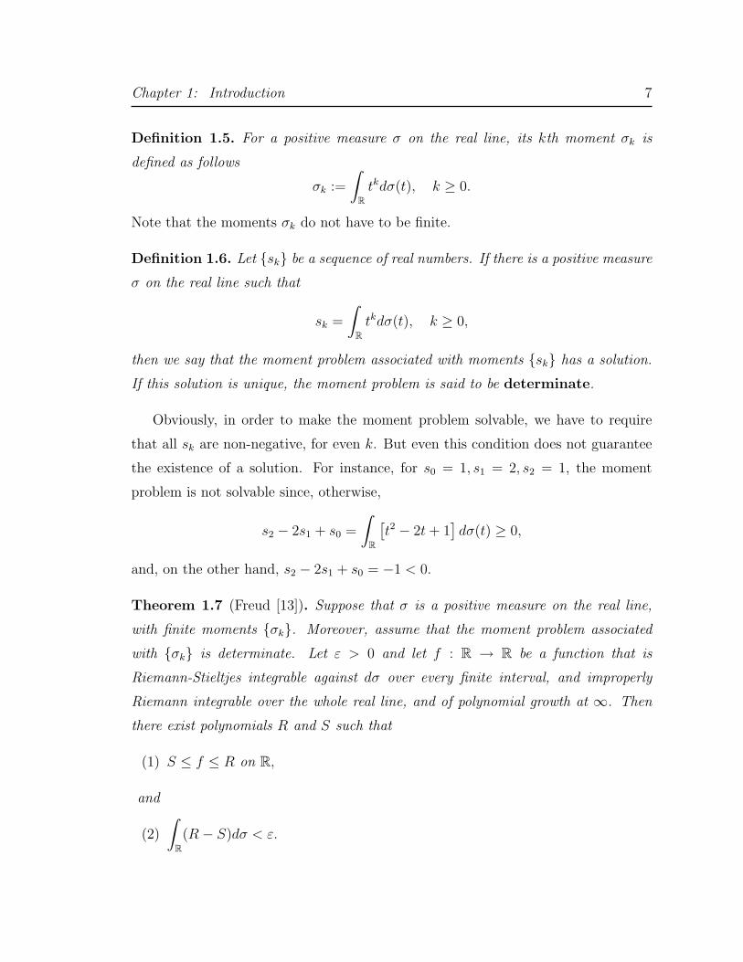
Definition 1.5. For a positive measure σ on the real line, its kth moment σk is

defined as follows

σk :=

∫Rtkdσ(t), k ≥ 0.

Note that the moments σk do not have to be finite.

Definition 1.6. Let sk be a sequence of real numbers. If there is a positive measure

σ on the real line such that

sk =

∫Rtkdσ(t), k ≥ 0,

then we say that the moment problem associated with moments sk has a solution.

If this solution is unique, the moment problem is said to be determinate.

Obviously, in order to make the moment problem solvable, we have to require

that all sk are non-negative, for even k. But even this condition does not guarantee

the existence of a solution. For instance, for s0 = 1, s1 = 2, s2 = 1, the moment

problem is not solvable since, otherwise,

s2 − 2s1 + s0 =

∫R

[t2 − 2t+ 1

]dσ(t) ≥ 0,

and, on the other hand, s2 − 2s1 + s0 = −1 < 0.

Theorem 1.7 (Freud [13]). Suppose that σ is a positive measure on the real line,

with finite moments σk. Moreover, assume that the moment problem associated

with σk is determinate. Let ε > 0 and let f : R → R be a function that is

Riemann-Stieltjes integrable against dσ over every finite interval, and improperly

Riemann integrable over the whole real line, and of polynomial growth at ∞. Then

there exist polynomials R and S such that

(1) S ≤ f ≤ R on R,

and

(2)

∫R(R− S)dσ < ε.


Remark. If W is a weight function and dσ(t) = W (t)dt, the previous theorem

establishes a result on the one-sided L1 weighted polynomial approximation.

There is a certain connection between the theory of orthogonal polynomials and the

moment problem. So-called Hamburger’s and Carleman’s conditions are sufficient

for the moment problem to be solvable and determinate, respectively (see, e.g. [6]).

Chapter 2

Weighted unconstrained

polynomial approximation on the

real line

2.1 Rate of approximation

2.1.1 Notations and Definitions

Although Theorem 1.2 establishes the density of algebraic polynomials in the space

CW , another important question is about the rate of such approximation. In order to

state results in this direction, we first introduce some basic notations and definitions.

• Classes of Weights:

(1) We say that W : R→ (0, 1] is a general weight or general weight function

if W is continuous and satisfies conditions (i), (ii) of Theorem 1.2 as well

as

limx→±∞

xnW (x) = 0, n ≥ 0. (2.1)

(2) We say that W : R→ (0, 1] is a Freud-type weight if W (x) = exp(−Q(x)),

where Q is even and continuous on R, Q′′ is continuous on (0,∞), xQ′(x)

9

Chapter 2: Weighted unconstrained polynomial approximation on the real line 10

is positive and increasing in (0,∞) with limits 0 and ∞ at 0 and ∞,

respectively. In addition, for some A,B > 0,

A ≤ xQ′′(x)

Q′(x)≤ B, x ∈ (0,∞).

We denote by F the class of all Freud-type weights. Note that any Freud-

type weight is a general weight.

(3) Freud’s weights: Wα(x) = exp(−|x|α). Note that Wα ∈ F, for all α > 1.

• For any weight function W , recall that

CW := CW (R) = f ∈ C(R)∣∣ limx→±∞

f(x)W (x) = 0,

and ‖f‖W := ‖f‖CW := supx∈R |f(x)W (x)|.

• Let W be a weight function. For any function f such that ‖fW‖Lp(R) < ∞if p < ∞ and f ∈ CW if p = ∞, let En(f,W )p := infP∈Πn ‖(f − P )W‖Lp(R)

denote the value of best weighted approximation by polynomials of degree ≤ n

in the Lp-norm. For convenience, we denote En(f,W ) := En(f,W )∞.

• Recall that the Gamma and the Beta functions are defined as follows:

Γ(z) =

∫ ∞0

tz−1e−tdt, for Re z > 0,

and

B(x, y) =

∫ 1

0

tx−1(1− t)y−1dt, for Re x, Re y > 0.

2.1.2 Jackson-Favard inequality

Since the general weight function W decays rapidly to 0 (see condition (2.1)), it

turns out that the weighted norm of any polynomial outside of the fixed finite in-

terval can be estimated in terms of the weighted norm of this polynomial inside the

interval. These observations lead to a powerful tool in weighted approximation called

restricted range inequalities. We now introduce Freud’s and Mhaskar-Rakhmanov-

Saff’s numbers, which arise in these inequalities.


Definition 2.1. Let W ∈ F. For n ≥ 1, let qn be the positive root of equation

n = qnQ′(qn). (2.2)

Then qn is called nth Freud’s number. The positive root an of the equation

n =2

π

∫ 1

0

antQ′(ant)√

1− t2dt (2.3)

is called nth Mhaskar-Rakhmanov-Saff’s number.

Note that conditions on the function Q(x) guarantee existence and uniqueness of

such numbers. For instance, for Freud’s numbers, the function xQ′(x) is continuous

on (0,∞), and has limits 0 and ∞ at 0 and ∞, respectively. Therefore, by the

Intermediate Value Theorem, for all n ≥ 1, there exists a solution of n = xQ′(x)

while uniqueness is guaranteed by monotonicity of xQ′(x).

For Freud’s weights Wα(x) = exp(−|x|α), α ≥ 1, and n ≥ 1:

qn = (n/α)1/α, (2.4)

and

an =

(2α−2 Γ(α/2)2

Γ(α)

)1/α

n1/α. (2.5)

Indeed, for Q(x) = xα, α ≥ 1, x ≥ 0, equality (2.2) implies

n = qnαqα−1n ,

and so (2.4) follows. For Mhaskar-Rakhmanov-Saff’s numbers, recalling that

B(x, y) =Γ(x)Γ(y)

Γ(x+ y), Γ(z + 1) = zΓ(z), Γ(1/2) =

√π,

and using equality (2.3) together with the duplication formula Γ(z + 1/2) =


21−2z√πΓ(2z), we obtain

n =2

π

∫ 1

0

antQ′(ant)√

1− t2dt =

2αaαnπ

∫ 1

0

tα√1− t2

dt

[u = t2, dt =du

2√u

]

=αaαnπ

∫ 1

0

u(α−1)/2(1− u)−1/2du =αaαnπB

(α + 1

2,1

2

)=αaαnπ

Γ((α + 1)/2)Γ(1/2)

Γ(α/2 + 1)=αaαnπ

Γ(α + 1)π

2αΓ(α/2 + 1)2

=αaαnαΓ(α)

2α(α/2)2Γ(α/2)2=

aαnΓ(α)

2α−2Γ(α/2)2,

which implies (2.5). Observe that an and qn are both of order n1/α.

We are now ready to state a theorem which provides an estimate for the rate of

weighted (unconstrained) approximation of f in terms of the norm of its derivative.

Recall that a function f : [a, b] → R is said to be absolutely continuous on [a, b] if

for every ε > 0, there is a number δ > 0 such that whenever a sequence of pairwise

disjoint sub-intervals [xk, yk] of [a, b], k = 1, 2, . . . , n, satisfiesn∑k=1

|yk − xk| < δ then

n∑k=1

|f(yk) − f(xk)| < ε. Note that if f is absolutely continuous on [a, b], then its

derivative f ′ exists almost everywhere on [a, b] and is Lebesgue-integrable over [a, b].

Theorem 2.2 (Jackson-Favard inequality). Let α > 1, 1 ≤ p ≤ ∞ and f : R → Rbe absolutely continuous over each finite interval, with ‖f ′Wα‖Lp(R) <∞. Then

En(f,Wα)p ≤ C0ann‖f ′Wα‖Lp(R), (2.6)

where C0 does not depend on f and n.

This theorem was proved by Freud [14], [15] in the case α ≥ 2, and by Levin and

Lubinsky [21] in the case 1 < α < 2. It turns out that (2.6) is no longer valid in

the case α = 1, and therefore this case requires a separate consideration (for more

details see, for example, [22]).

Remark. Throughout this thesis, by C we denote a positive constant, which does

not depend on f and n (and may be different even when they appear in the same

line). By C0, C1, C2, . . . we denote constants which are used more than once.


As a consequence of (2.6), one can derive an estimate for the rate of weighted

approximation of f in terms of f ′. For any polynomial Pn ∈ Πn,

En(f,Wα)p = En(f − Pn,Wα)p ≤ C0ann‖(f ′ − P ′n)Wα‖Lp(R).

This immediately yields

En(f,Wα)p ≤ C0annEn−1(f ′,Wα)p, 1 ≤ p ≤ ∞.

Using iteration, the following corollary followa:

Corollary 2.3. Let α > 1, 1 ≤ p ≤ ∞, r ∈ N. Assume that the (r − 1)-th derivative

of f is locally absolutely continuous and ‖f (r)Wα‖Lp(R) <∞. Then

En(f,Wα)p ≤ Cr0

(ann

)r‖f (r)Wα‖Lp(R).

2.1.3 Jackson Theorem

It is well known that there exist differentiable functions that do not have bounded

derivatives, as well as continuous functions which are not differentiable at all. For

example, the function

f(x) =

x2 sin

(1

x2

), x ∈ R \ 0,

0, x = 0,

is differentiable on R, but f ′ is unbounded in the neighbourhood of x = 0. Thus

‖f ′‖Wα = ∞ and therefore we cannot apply the result of Theorem 2.2. How is it

possible to establish the rate of approximation for such class of functions?

In the case of approximation on an interval, introduction of moduli of continu-

ity and moduli of smoothness by Lebesgue (1909) and De la Vallee Poussin (1919)

resolved this problem. Since then, this tool has been widely used by many mathe-

maticians in different areas and still is in use today. Let

∆rhf(x) :=

r∑k=0

(−1)r−k(r

k

)f(x+ kh), r ∈ N,


be the rth (forward) difference. For a function f ∈ C[a, b], the modulus of

smoothness of order r is defined as follows:

ωr(f ; t) := ω(t; f ; [a, b]) :=

suph∈[0,t]

maxx∈[a,b−rh]

|∆rhf(x)|, t ∈ [0, (b− a)/r],

ω((b− a)/r; f ; [a, b]), t > (b− a)/r.

One can now estimate the rate of approximation of any continuous function in terms

of the above moduli. Such estimates are also called Jackson-type estimates (inequal-

ities).

Theorem 2.4 (Classical Jackson). Let r be a positive integer. Then, for any f ∈C[a, b],

En(f) ≤ C(r)ωr((b− a)/n, f, [a, b]), n ≥ r − 1,

where the constant C(r) depends only on r.

A similar tool and approach is going to be used in our case. For r ≥ 1, define the

rth order weighted modulus of smoothness (with the weight Wα) as follows:

ωr,p(f,Wα, t) := sup0<h≤t

‖(∆rhf)Wα‖Lp[−h1/(1−α),h1/(1−α)]

+ infP∈Πr−1

‖(f − P )Wα‖Lp(R\[−t1/(1−α),t1/(1−α)]).

These moduli were first introduced in the early works of Freud, and then were

used by Ditzian and Totik [11] and Mhaskar [24]. Note that if f is a polynomial of

degree < r, then ωr,p(f,Wα, t) is identically zero. In fact, the weighted moduli can

be defined for wider class of weights from F as well (see, for example, survey [22]).

In order to describe the behavior of moduli ωr,p, recall their basic properties (see

e.g. [9, 10]):

Properties of weighted moduli of smoothness on the real line:

Let α > 1, 1 ≤ p ≤ ∞. Suppose that f ∈ CWα if p = ∞, and fWα ∈ Lp(R) if

p <∞. Then

(i) ωr,p(f,Wα, t) is non-decreasing on [0,+∞).

(ii) limt→0+

ωr,p(f,Wα, t) = 0.


(iii) ωr,p(f,Wα, 2t) ≤ Cωr,p(f,Wα, t), t ≥ 0, where C is a positive constant inde-

pendent of f and t.

(iv) If f (r−1) is locally absolutely continuous and f (r)Wα ∈ Lp(R), then ωr,p(f,Wα, t) ≤Ctr‖f (r)Wα‖Lp(R), t ≥ 0, where C is a positive constant independent of f and

t.

(v) If r > 1, then ωr,p(f,Wα, t) ≤ Cωr−1,p(f,Wα, t), t ≥ 0, where C is a positive

constant independent of f and t.

(vi) Assume that a Markov-Bernstein inequality holds, i.e.,

‖PWα‖Lp(R) ≤ Cn

an‖P ′Wα‖Lp(R),

for all n ≥ 1 and any polynomial P ∈ Πn. Then the Marchaud-type inequality

is true

ωr,p(f,Wα, t) ≤ Atr[∫ B

1

ωr+1,p(f,Wα, u)

ur+1du+ ‖fWα‖Lp(R)

],

for some A,B > 0 independent of f and t.

Remark. For Freud’s weights Wα and 1 ≤ p < ∞, the Markov-Bernstein

inequality holds for α > 1. It was proven by Nevai and Lubinsky in 1987. If

p = ∞, the Markov-Bernstein inequality holds for α ≥ 1 (see, for example,

[24]).

(vii) Suppose that for some 0 < δ < r, ωr,p(f,Wα, t) = O(tδ), t→ 0 + . Let k := [δ]

(integer part of δ). Then f (k) exists a.e. on R, and

ωr−k,p(f(k),Wα, t) = O(tδ−k), t→ 0 + .

If p =∞, f (k) is continuous on R.

The following result is an analogue of the classical Jackson theorem (for finite

intervals) for weighted polynomial approximation on the real line.


Theorem 2.5 (Jackson-type inequality, see e.g. [22]). Let α > 1 and r ≥ 1. If

f ∈ CWα, for p =∞, and fWα ∈ Lp(R), for p <∞, then,

En(f,Wα)p ≤ Cωr,p(f,Wα,ann

), n ≥ r − 1

where C is a positive constant independent of f and n.

Under conditions of Property (vi), i.e., if the Markov-Bernstein inequality holds,

a converse Bernstein-type theorem has the following form (see [9]):

Theorem 2.6. Let 0 < δ < r. Then

ωr,p(f,Wα, t) = O(tδ), t→ 0+⇐⇒ En(f,Wα)p = O((ann

)δ), n→∞.

The previous result provides a constructive characterization of Lipschitz-type

classes in terms of the rate of weighted approximation. Once we know that a function

is smooth enough, we can guarantee a certain rate of approximation, and conversely, if

the convergence of En(f,Wα)p to 0 is sufficiently fast, then it is possible to determine

how smooth the function is.

2.2 Restricted Range Inequalities

Restricted range inequalities play an important role in weighted approximation. For

instance, one uses this tool in order to prove the Jackson-type inequality. According

to Paul Nevai, Freud’s discovery of these inequalities is one of the most significant

of Freud’s contributions to weighted approximation theory.

The following theorem deals with the case p =∞, and will be used in Chapter 4.

Theorem 2.7 (Freud [13]). Let α ≥ 1. Then, for any n ≥ 1 and polynomial P ∈ Πn,

‖PWα‖L∞(R) = ‖PWα‖L∞[−4q2n,4q2n].

Since one of the intermediate steps in the proof of this theorem will be used later,

we mention the main ideas of this proof following [22]. By Tn, we denote the classical


Chebyshev polynomial of degree n, i.e., Tn(x) := cos(n arccosx), x ∈ [−1, 1] (and

uniquely extended to the whole real line).

Proof. We use the fact (see, for example, [24]) that for any polynomial P ∈ Πn,

|Pn(x)| ≤ Tn(|x|)‖P‖L∞[−1,1] ≤ (2|x|)n‖P‖L∞[−1,1], |x| ≥ 1.

Scaling from the interval [−1, 1] to [−q2n, q2n], we get

|Pn(x)| ≤(

2|x|q2n

)n‖P‖L∞[−q2n,q2n] ≤

(2|x|q2n

)nW−1α (q2n)‖PWα‖L∞[−q2n,q2n], |x| ≥ q2n,

where the last inequality follows from the monotonicity of Wα(x) on (0,∞).

Hence,

|Pn(x)Wα(x)| ≤ 2n|x|nWα(x)

qn2nW−1α (q2n)‖PWα‖L∞[−q2n,q2n].

In addition, if x ≥ 4q2n, then

log|x|nWα(x)

qn2nW−1α (q2n) =

∫ x

q2n

n− αuα

udu ≤ −n

∫ 4q2n

q2n

du

u= −n log 4,

since αuα is an increasing function on (0,∞), and αqα2n = 2n.

Together with the previous inequalities this implies that for x ≥ 4q2n,

|Pn(x)Wα(x)| ≤ 2−n‖PWα‖L∞[−q2n,q2n]. (2.7)

For negative values of x, it is enough to consider the polynomial Q(x) := P (−x),

and apply (2.7) for Q. Thus,

‖PWα‖L∞(R) = ‖PWα‖L∞[−4q2n,4q2n].

The proof of Theorem 2.7 shows the exponential decay of PWα outside the interval

[−4q2n, 4q2n], depending on the value of n. An analogue of Theorem 2.7 takes place

in the Lp-spaces [22]:

Theorem 2.8. For any p > 0,α ≥ 1,

‖PnWα(x)‖Lp(R) ≤ (1 + e−An)‖PWα‖Lp[−Bq2n,q2n], (2.8)

where A > 0 and B is large enough.


According to the previous theorem, the Lp norm of the weighted polynomials

“lives” inside the intervals [−Bq2n, Bq2n], with appropriate B. A natural question

arises: what is the best (smallest) B? This problem is deeply discussed in the

monograph of Saff and Totik [30] for general weights. The case of exponential weights

is treated in [24]. The following result allows us to write a strict inequality in (2.8)

(see [24]):

Theorem 2.9. Let W ∈ F, 0 < p <∞ and let P be a polynomial of degree ≤ n+2/p,

which is not identically zero. Then

‖PW‖Lp(R\[−an,an]) < ‖PW‖Lp[−an,an],

and

‖PW‖Lp(R) < 21/p‖PW‖Lp[−an,an],

where an denotes the nth Mhaskar-Rakhmanov-Saff’s number.

Chapter 3

One-Sided Lp Methods

3.1 Freud and Nevai’s One-sided L1 method

One of the methods in proving weighted Jackson-type Theorems is the one-sided L1

method developed by Freud and Nevai. Usually, the L1 method allows to obtain

estimates on the rate of approximation of special functions such as characteristic

functions. After that, using duality and other tools, one can get necessary estimates

in the Lp-spaces, 1 < p ≤ ∞. However, using this approach one loses the property

of one-sidedness, and therefore, this approach is not useful for our purposes. Hence,

we only discuss the L1 method.

Mainly, this method is based on the theory of orthogonal polynomials and Gaus-

sian quadratures. Some important definitions and theorems on this subject are stated

below. A nice survey of this material could be found in Mhaskar’s monograph [24].

For a given general weight function W , define orthonormal polynomials p0, p1, ...

by

pn(x) = pn(W 2, x) = γnxn + . . . , γn > 0,

and such that ∫Rpn(x)pm(x)W 2(x)dx = δmn, (3.1)

where δmn is the Kronecker δ-function, i.e., δmn = 0, if m 6= n, and δmn = 1, if

m = n.

19

Chapter 3: One-Sided Lp Methods 20

Remark. We use the weight W 2 and not W in the definition of orthonormal poly-

nomials. This convention simplifies some formulations later on.

Note that each pn has exactly n simple real zeroes. Indeed, otherwise, pn has at

most n − 1 distinct odd order zeroes y1, . . . , ym, m ≤ n − 1. Then the polynomial

p(x) :=m∏i=1

(x − yi) (p(x) := 1 if m = 0) is of degree less than n and p(x)pn(x) ≥ 0,

for all x ∈ R. Hence, ∫Rp(x)pn(x)W 2(x)dx > 0.

On the other hand, it is well known that the system of orthonormal polynomials

p0, . . . , pn−1 is a basis in Πn−1 (see, for example, [24]). This together with (3.1)

implies that ∫Rp(x)pn(x)W 2(x)dx = 0.

This contradiction yields that pn has exactly n simple zeroes. Denote them by

xnn < x(n−1)n < · · · < x2n < x1n.

Then the nth Christoffel function for W 2 is defined as follows

λn(W 2, x) = infP∈Πn−1

∫R(P (x)W (x))2dx

P 2(x).

As was already mentioned, the system of orthonormal polynomials p0, . . . , pn−1 is

a basis for the space Πn−1. Hence, for any P ∈ Πn−1, we may write

P (x) =n−1∑j=0

cjpj(x), x ∈ R.

Then, using Parseval’s identity, we have∫RP 2(x)W 2(x)dx =

n−1∑j=0

c2j .

Now, Cauchy-Schwarz inequality implies that∫R(P (x)W (x))2dx

P 2(x)=

∫R(P (x)W (x))2dx(n−1∑j=0

cjpj(x)

)2 ≥

n−1∑j=0

c2j

n−1∑j=0

p2j(x)

n−1∑j=0

c2j

=1

n−1∑j=0

p2j(x)

.


Moreover, for any fixed x = x0, if P (x) = kn−1∑j=0

pj(x0)pj(x) for some constant k 6= 0,

then the last inequality becomes equality at x = x0. Thus we proved the following

identity for the Christoffel function

λn(W 2, x) =1

n−1∑j=0

p2j(x)

.

Recall now (see e.g. [19]) that the Gaussian quadrature formula∫Rf(x)W 2(x)dx ≈

n∑j=1

λn(W 2, xjn)f(xjn),

is exact for all polynomials P ∈ Π2n−1 ([24, p.10] ). As an application of the quadra-

ture formula, one can prove the following estimate known as the Posse inequality

(see e.g. [24, Theorem 1.2.3]): for any function f such that its first 2n−1 derivatives

are positive on (−∞, xkn),

n∑j=k+1

λn(W 2, xjn)f(xjn) ≤∫ xkn

−∞f(x)W 2(x)dx ≤

n∑j=k

λn(W 2, xjn)f(xjn).

This can be used to estimate the error of one-sided approximation of characteristic

functions. For A a subset of R, denote

χA(x) :=

1, if x ∈ A,

0, otherwise.

We have the following result.

Lemma 3.1 (see Mhaskar [24, Corollary 1.2.6]). Let W be a general weight function,

n ≥ 1, and ξ ∈ (x(k+1)n, xkn), where x(k+1)n and xkn are the consecutive zeroes of pn.

Then there exist two polynomials Rξ and rξ such that

rξ ≤ χ(−∞,ξ] ≤ Rξ on R,

and ∫R[Rξ(x)− rξ(x)]W 2(x)dx ≤ λn(W 2, xkn) + λn(W 2, x(k+1)n).


Thus, upper estimates for the Christoffel functions immediately yield bounds for

the error of one-sided polynomial approximation. There are several different ways

to estimate Christoffel functions (see, for instance, [26]). For our purposes, we only

mention one quite simple method introduced by Freud [13].

Lemma 3.2 ([22, Lemma 4.2]). If α > 1, then there exist C1, C2 > 0 such that, for

n ≥ 1 and |ξ| ≤ C1an,

λn(W 2α, ξ) ≤ C2

annW 2α(ξ).

Using results of Lemmas 3.1 and 3.2, we follow Lubinsky [22] and construct one-

sided L1 approximation for a special class of functions (of polynomial growth at

infinity).

Theorem 3.3 ([22, Theorem 4.3]). Let α > 1, and let f be of polynomial growth

at ∞. Moreover, suppose that f ′ is continuous, and f ′W 2α ∈ L1(R). Then, for any

n ∈ N, there exist polynomials pn and pn of degree ≤ n such that

pn ≤ f ≤ pn on R,

and∫R(pn(x)− pn(x))W 2

α(x)dx ≤ Cann

(∫R|f ′(x)|W 2

α(x)dx+ ‖f ′W 2α‖L∞(|x|≥Can)

).

Proof. We prove this theorem under the assumption that f ′ is nonnegative on the

real line and moreover, supp(f ′) ⊂ (xnn, x1n), i.e., f ′ = 0 outside (xnn, x1n), where

xnn, x1n are the smallest and the largest zeros of pn(W 2α, x)), respectively. By the

Fundamental Theorem of Calculus

f(x) =f(0) +

∫ x

0

f ′(ξ)dξ

=f(0) +

∫ ∞0

(1− χ(−∞,ξ)(x))f ′(ξ)dξ −∫ 0

−∞χ(−∞,ξ)(x)f ′(ξ)dξ.

Now, using polynomials Rξ and rξ from Lemma 3.1, define

pn(x) = f(0) +

∫ ∞0

(1− rξ(x))f ′(ξ)dξ −∫ 0

−∞rξ(x)f ′(ξ)dξ,


and

pn(x) = f(0) +

∫ ∞0

(1−Rξ(x))f ′(ξ)dξ −∫ 0

−∞Rξ(x)f ′(ξ)dξ.

Conditions f ′ ≥ 0 and rξ ≤ χ(−∞,ξ) ≤ Rξ immediately yield that pn ≤ f ≤ pn on the

whole real line. Observing that

(pn − pn)(x) =

∫R(Rξ − rξ)(x)f ′(ξ)dξ,

we conclude∫R(pn(x)− pn(x))W 2

α(x)dx ≤∫

R

[∫R(Rξ(x)− rξ(x))W 2

α(x)dx

]f ′(ξ)dξ.

Now, Lemmas 3.1 and 3.2 imply that for at least |ξ| ≤ C1an (note that the largest

zero x1n is of the same order as an),∫R(Rξ(x)− rξ(x))W 2(x)dx ≤ C2

annW 2(ξ).

Hence,∫R(pn(x)− pn(x))W 2

α(x)dx ≤ C2ann

∫ C1an

−C1an

f ′(ξ)W 2α(ξ)dξ

+ ‖f ′W 2α‖L∞(|x|≥C1an)

∫|ξ|>C1an

[W−2α (ξ)

∫R(Rξ(x)− rξ(x))W 2

α(x)dx

]dξ.

The first term on the right-hand side has the required form. Using estimates for

Christoffel functions, which are given in details in [16], [24, p.83], one can complete

the proof of the theorem.

Remark. Under the conditions of the previous theorem ‖f ′W 2α‖L∞(|x|≥Can) does not

have to be finite. It is possible to construct a counterexample.

Recall that a function f : [a, b]→ R is said to be of bounded variation if

supn≥1

supa≤x0<...<xn≤b

n∑i=1

|f(xi)− f(xi−1)| <∞.

In 1974, using the same approach as in the proof of the previous theorem Freud

proved the following result.


Theorem 3.4 (Freud [12, p.297]). Let W ∈ F. Assume that for some a, b > 0,

1 + a <Q′(2x)

Q′(x)< 1 + b.

Let r ≥ 0 and f (r) be of bounded variation over every finite interval, and of polynomial

growth at ∞, satisfying for some A,B > 0 and integer m, |f(x)| ≤ A+Bx2m. Then

there exist polynomials pn and pn from Πn such that

pn ≤ f ≤ pn on R, (3.2)

and∫R(pn(x)− pn(x))W 2(x)dx ≤ C

(ann

)r+1(∫

RW 2(x)df (r)(x) + A+B

), (3.3)

where the constant C is independent of f, n, A,B.

Remark 1. The weights Wα = exp(−|x|α), α > 1 satisfy the conditions of Theorem

3.4.

Remark 2. Theorem 3.4 implies an estimate for the rate of unconstrained approx-

imation:

En(f,W 2)1 ≤ C(ann

)r+1(∫

RW 2(x)df (r)(x) + A+B

).

These estimates can be extended to other Lp-spaces, using duality (see e.g. [22]).

3.2 Partially one-sided polynomial approximation

on the real line and its applications

In [23], Mastroianni and Szabados proved a similar result to Theorem 3.4 for a wider

class of functions. Namely, they constructed one-sided approximants for the functions

of exponential growth and presented estimates for the rate of this approximation in

the Lp-norm (1 ≤ p ≤ ∞). The main generalization is that not only functions of

polynomial growth are allowed. On the other hand, the restriction made in [23] is

requiring (3.2) to hold only on some finite intervals instead of the whole real line.

This restriction is necessary in order to include functions of exponential growth.


Obtained results can be used in the applications (estimating the ordinary weighted

best polynomial approximation, Lagrange interpolation, quadrature errors).

3.2.1 Estimates for certain classes of functions

Let W ∈ F be a Freud-type weight, W (x) = exp(−Q(x)). Recall that Mhaskar-

Rakhmanov-Saff numbers an are defined by (2.3), and by x1n > · · · > xnn denote

roots of n-th orthonormal polynomial pn(W ) with respect to W 2.

Theorem 3.5 ([23, Theorem 1]). Let r ≥ 0 be an integer, and let f be such that f (r)

is of bounded variation on each finite subinterval of R. If

n(r+1)/3

∫|t|≥x1n/2

W 2|df (r)(t)| ≤ C

∫RW 2(t)|df (r)(t)| <∞, n ≥ 1, (3.4)

with some absolute constant C > 0, then there exist polynomials rn, Rn ∈ Π2n−1 such

that

rn(x) ≤ f(x) ≤ Rn(x), if |x| ≤ x1n, n ≥ 1,

and

‖(Rn − rn)W 2‖Lp(R) =O

((ann

)r+1/p)∫

RW 2(t)|df (r)(t)|, 1 ≤ p ≤ ∞.

Remark 1. Theorem 1 does not establish a convergent to 0 estimate in the case

r = 0 and p =∞.

Remark 2. Note that condition (3.4) is rather weak, and the class of functions of

exponential growth which satisfy it, is quite rich.

However, when the derivative of the function is not of bounded variation, Theorem

3.5 can’t be applied. The following theorem resolves this problem.

Theorem 3.6 ([23, Theorem 2]). Let r ≥ 1 be an integer, 1 ≤ p ≤ ∞, 0 < µ < 1,

let

bn := an

(1 + λr

(log n

n

)2/3), (3.5)


where λr > 0 is a suitable constant, and let f be such that

exp(γn1/3) max1≤j≤r

‖f (j)W 2‖Lp(|x|≥µan) ≤ ‖f (r)W 2‖Lp(R) <∞, n ≥ 1, (3.6)

with a suitable constant γ > 0. Then there exist polynomials Rn, rn ∈ Π2n−1 such

that

rn(x) ≤ f(x) ≤ Rn(x), if |x| ≤ bn, n ≥ 1

and

‖(Rn − rn)W 2‖Lp(R) =Cr

(ann

)rmax1≤j≤r

‖f (j)W 2‖Lp(R).

In the case p = 1, condition (3.6) is more restrictive than (3.4) in general, since it

requires an “exponential” estimate in the inequality, and not “polynomial” as (3.4)

does. However, (3.6) still allows functions like f(x) = exp(2Q(x)−νQ(x)1/3) (ν > γ),

with exponential growth at ∞.

3.2.2 Applications

In [23], Mastroianni and Szabados also present some applications of obtained results.

Below, the weight function W ∈ F.

As was mentioned before, the following quadrature formula∫Rf(x)W 2(x)dx ≈

n∑k=1

λknf(xk),

becomes an equality whenever f is a polynomial of degree ≤ 2n−1 and xk are zeroes

of pn(W 2). The coefficients

λkn :=

∫Rlkn(x)W 2(x)dx,

where

lkn(x) :=pn(W 2, x)

p′n(W 2, xk)(x− xk),

are called Cotes numbers of the quadrature procedure with respect to weight W 2.

More detailed treatment on this topic can be found in [24, pp.11–13].


The following corollary provides an estimate of the error of such quadrature

formula

en(f) := en(f,W 2) =

∣∣∣∣∣∫

Rf(x)W 2(x)dx−

n∑k=1

λknf(xk)

∣∣∣∣∣ .Corollary 3.7 (Quadrature formula). If ‖f (r)W 2‖L1(R) < ∞ and (3.6) holds with

p = 1, then

en(f) ≤ C(ann

)rmax1≤j≤r

‖f (j)W 2‖L1(R).

Another applications describes the rate of Lagrange interpolation in the L2-

metric.

Definition 3.8. A Lagrange polynomial

L(z; f) := L(z; f ; z1, z2, . . . , zm)

that interpolates a function f at points z1, z2, . . . , zm (interpolation nodes) is defined

as an algebraic polynomial of at most mth order that takes the same values at these

points as the function f , i.e.,

L(zi; f) = f(zi), i = 0, . . . ,m.

Let Ln(f,W ) be the Lagrange interpolation polynomial with nodes at zeroes of

pn(W ). Then the following estimate is valid:

Corollary 3.9 (L2-Lagrange interpolation). If ‖f (r)‖L2(R) < ∞, r ≥ 1, and (3.6)

holds with p = 2 and 0 ≤ j ≤ r, then

‖(f − Ln(f,W ))W‖L2(R) = O((an

n

)r)max1≤j≤r

‖f (j)W‖L2(R).

Chapter 4

One-Sided L∞ Weighted

Approximation

As we have discussed after Question 1.3, direct generalization of the problem of one-

sided approximation on an interval to the problem of one-sided approximation on the

whole real line becomes ill-posed. Therefore, we repose the problem in the following

way.

Problem 4.1. Problem definition:

Does there exist a system of intervals [−dn, dn], n ≥ 1 such that

Condition A. dn →∞, n→∞;

Condition B. For each function f ∈ CWα , α ≥ 1, there exists a sequence of poly-

nomials Pn ∈ Πn, n ≥ 1 such that limn→∞

‖f − Pn‖Wα = 0, and Pn(x) ≥ f(x)

(Pn(x) ≤ f(x)), for all x ∈ [−dn, dn]?

Further, we present the largest possible in some sense sequence of dn, so that

Problem 4.1 has a positive answer. Recall that α ≥ 1 is a parameter in the weight

Wα = exp(−|x|α).

Lemma 4.2. If the sequence dn∞n=1 is such that Condition B is satisfied, then

dn < C3nα, for all n ≥ 1, and for some constant C3 > 0.

28

Chapter 4: One-Sided L∞ Weighted Approximation 29

Proof. Recall that qn := (n/α)1/α, n ≥ 1, is Freud’s number (see (2.4)). We will

prove that dn < 4q2n.

Suppose to the contrary that, for all functions f ∈ CWα and all ε > 0, there

exists n ∈ N and a polynomial Pn of degree ≤ n such that ‖f − Pn‖Wα < ε, and

Pn(x) ≥ f(x), for all x ∈ [−4q2n, 4q2n].

Consider the function

f ∗(x) :=

(1

2

)α(|x|/4)α/4

(Wα(x))−1, x ∈ R,

which is clearly from CWα . Then, there exist n ∈ N and a polynomial P ∗n ∈ Πn such

that ‖f ∗ − P ∗n‖Wα < 1/4 and P ∗n(x) ≥ f ∗(x), for all x ∈ [−4q2n, 4q2n]. In particular,

P ∗n(4q2n)Wα(4q2n) ≥ f ∗(4q2n)Wα(4q2n) =1

2n/2. (4.1)

Now, using restricted range inequality (2.7), we get

P ∗n(4q2n)Wα(4q2n) ≤ 1

2n‖P ∗nWα‖L∞[−q2n,q2n]. (4.2)

Note that

‖P ∗nWα‖L∞[−q2n,q2n] ≤ ‖f ∗ − P ∗n‖Wα + ‖f ∗‖Wα = 1/4 + 1 = 5/4, (4.3)

since maxx∈R

f ∗(x)Wα(x) = f ∗(0)Wα(0) = 1.

Inequalities (4.1),(4.2) and (4.3) imply

1

2n/2≤ 5

2n+2,

which is not true for any n ≥ 1. This contradiction completes the proof.

Note that one can use the function f = −f ∗ in order to obtain the same result

for approximation from below.

We now prove an auxiliary lemma, which will be used in the proofs of the positive

results.

Lemma 4.3. For all α > 1, there exists a positive constant C4 = C4(α) and a

sequence of polynomials Qn ∈ Πn, n ≥ 1 such that


(1) Qn(x) ≥ (Wα(x))−1, for x ∈ [−C4n1/α, C4n

1/α],

and

(2) supn≥1‖Qn‖Wα <∞.

Proof. Define the function f as follows

f(x) :=

(Wα(x))−1, if |x| ≤ λan,

(Wα(λan))−1, if |x| > λan,

where an represents nth Mhaskar-Rakhmanov-Saff’s number defined by equality (2.5)

(an = Ln1/α, L = L(α)), and the parameter λ is to be chosen. Obviously, f is

absolutely continuous over each finite interval and ‖f ′Wα‖L∞(R) < ∞. Hence, one

can apply Theorem 2.2 in order to estimate the rate of approximation of f by Πn:

En(f,Wα) ≤ C0ann‖f ′Wα‖L∞R = C0

ann‖α|x|α−1‖L∞[−λan,λan]

= C0annαλα−1(an)α−1 = αC0λ

α−1aαn

n= αC0L

αλα−1,

and since λα−1 → 0, λ→ 0, we can now choose λ so that

En(f,Wα) = ‖f − Pn‖Wα < 1/2, (4.4)

for some polynomial Pn of degree ≤ n. Therefore, for |x| ≤ λan, we have

|(f(x)− Pn(x))Wα(x)| < 1/2,

which implies

|1− Pn(x)Wα(x)| < 1/2.

Hence

1/2 < Pn(x)Wα(x) < 3/2,

and so for Qn := 2Pn,

Qn > (Wα)−1 on [−λan, λan], and ‖QnWα‖L∞[−λan,λan] < 3.


Finally, for |x| > λan,

|Qn(x)Wα(x)| ≤ 2(|(Pn(x)− f(x))Wα(x)|+ |f(x)Wα(x)|)

< 2(1/2 + 1) = 3.

Note that our approach fails for α = 1.

The following lemma together with Lemma 4.2 prove that dn ∼ n1/α are asymp-

totically the largest possible.

Theorem 4.4. For all α > 1, there exist C4 = C4(α) > 0 such that the system of

intervals [−C4n1/α, C4n

1/α], n ≥ 1 satisfies both Conditions A and B of Problem

4.1.

Proof. Clearly, we only need to prove that Condition B is satisfied for some constant,

whereas Condition A always holds for chosen system of intervals. We use the same

constant C4 introduced in Lemma 4.3.

Let f ∈ CWα be fixed. There exists a sequence of polynomials Pn ∈ Πn, n ≥ 1such that ‖f−Pn‖Wα = En(f,Wα). The polynomialRn(x) := Pn(x)+En(f,Wα)Qn(x)

is of degree ≤ n, where Qn are polynomials constructed in Lemma 4.3. We will now

show that the sequence of polynomials Rn satisfies Condition B, with dn = C4n1/α.

Indeed,

‖f −Rn‖Wα ≤ ‖f − Pn‖Wα + En(f,Wα)‖Qn‖Wα ≤ 4En(f,Wα), (4.5)

which implies that ‖f − Rn‖Wα → 0, n → ∞, since En(f,Wα) → 0, n → ∞, for all

f ∈ CWα .

It remains to show that Rn lies above f on [−C4n1/α, C4n

1/α]. Indeed,

Rn(x)− f(x) = Pn(x)− f(x) + En(f,Wα)Qn(x)

≥ En(f,Wα)Qn(x)− (Wα(x))−1|(Pn(x)− f(x))Wα(x)|

≥ En(f,Wα)(Qn(x)− (Wα(x))−1) ≥ 0,

since Qn(x) > (Wα(x))−1 on [−C4n1/α, C4n

1/α] by Lemma 4.3.

The proof of Theorem 4.4 is now complete.


Inequality (4.5) implies the following Jackson-type estimate for this kind of ap-

proximation.

Corollary 4.5. Let α > 1 and f ∈ CWα. Then, for every n ∈ N, there exists a

polynomial Rn ∈ Πn such that

(1) ‖f − Rn‖Wα ≤ C5ωr,p(f,Wα,ann

), where the constant C5 is independent of f

and n (but depends on α),

(2) Rn(x) ≥ f(x), for all x ∈ [−C4n1/α, C4n

1/α].

Using Lemma 4.4, one can establish a similar result in the weighted Lp norm for

a certain class of functions.

Corollary 4.6. Let α > 1, 0 < p < ∞, and ε > 0. Suppose that f is a continuous

function with f 1+ε ∈ CWα. Then there is a sequence of polynomials Pn ∈ Πn, n ≥ 1and a constant C6 = C6(α) > 0 such that

(1) limn→∞

‖(f − Pn)Wα‖Lp(R) = 0,

and

(2) for all n ≥ 1, Pn(x) ≥ f(x), x ∈ [−C6n1/α, C6n

1/α].

Proof. Note that the condition f 1+ε ∈ CWα implies:

lim|y|→∞

|f((1 + ε)1/αy

)|e−|y|α = lim

|y|→∞

(|f((1 + ε)1/αy

)|1+εe−|(1+ε)1/αy|α

) 11+ε

= 0,

and therefore by Theorem 4.4 there exists a sequence of polynomials Rn ∈ Πn such

that

limn→∞

supy∈R|f((1 + ε)1/αy

)−Rn(y)|Wα(y) = 0, (4.6)

and for any n ∈ N ,

Rn(y) ≥ f((1 + ε)1/αy

), y ∈ [−C4n

1/α, C4n1/α]. (4.7)


Define Pn(x) = Rn

((1 + ε)−1/αx

), n ≥ 1, and denoting x := (1+ε)1/αy and using

(4.6), we get condition

‖(f − Pn)Wα‖Lp(R)

=

(∫R

[|f(x)−Rn

((1 + ε)−1/αx

)| exp(−|x|α)

]pdx

)1/p

=

(∫R(1 + ε)1/α

[|f((1 + ε)1/αy

)−Rn(y)| exp (−(1 + ε)|y|α)

]pdy

)1/p

≤ (1 + ε)1/(αp)‖f((1 + ε)1/αy

)−Rn(y)‖Wα

(∫R

exp(−εp|y|α)dy

)1/p

→ 0, n→∞,

and so (1) is verified. Inequality (4.7) now implies that for all n ≥ 1 and |x| ≤C4(1 + ε)1/αn1/α,

Pn(x) = Rn

((1 + ε)−1/αx

)≥ f

((1 + ε)1/α(1 + ε)−1/αx

)= f(x),

which verifies part (2) of the corollary. The proof is now complete.

Chapter 5

Conclusions

In this thesis, we solved the problem dealing with partially one-sided approximation

in the space CWα , α > 1. We are only aware of one paper on this subject [23] that

contains estimates of such approximation in the weighted Lp norms, but does not

establish the density of polynomials in the most general case. It uses technique and

theory of orthogonal polynomials. In this thesis, a different approach is presented,

which allows to obtain the same rate of partially one-sided approximation as the rate

of arbitrary unconstrained approximation.

It is worth mentioning that the case α = 1 still requires a separate consideration.

Also, a generalization of obtained asymptotical results to the Lp-spaces is a natural

problem. These problems are still open and deserve further investigation.

34

Bibliography

[1] N. I. Akhiezer, Lectures on Approximation Theory , Nauka, Moscow, 1965 [in Russian].

[2] A. Andreev, V. A. Popov, and Bl. Sendov, Jackson’s type theorems for onesided polynomial

and spline approximation, C. R. Acad. Bulgare Sci. 30 (1977), 1533–1536.

[3] S. N. Bernstein, Le probleme de lapproximation des fonctions continues sur tout laxe reel et

lune de ses applications, Bull. Math. Soc. France 52 (1924), 399–410.

[4] S. Bernstein, Demonstration du theoreme de Weierstrass fondee sur le calcul des probabilites,

Comm. Soc. Math. Kharkow 13 (1912/13), 1–2.

[5] Borel E., Lecons sur les Fonctions de Variables Reeles, Gauthier-Villars, Paris, 1905.

[6] T. S. Chihara, Hamburger moment problems and orthogonal polynomials, Trans. Amer. Math.

Soc. 315 (1989), 189–203.

[7] Ronald DeVore, One-sided approximation of functions, J. Approximation Theory 1 (1968),

11–25.

[8] Ronald A. DeVore and George G. Lorentz, Constructive approximation, Grundlehren der Math-

ematischen Wissenschaften [Fundamental Principles of Mathematical Sciences] 303 (1993),

x+449.

[9] Z. Ditzian and D. S. Lubinsky, Jackson and smoothness theorems for Freud weights in Lp (0 <

p ≤ ∞), Constr. Approx. 13 (1997), 99–152.

[10] Z. Ditzian and S. Tikhonov, Ulyanov and Nikolskii-type inequalities, J. Approx. Theory 133

(2005), 100–133.

[11] Z. Ditzian and V. Totik, Moduli of smoothness, Springer, 1987.

[12] Geza Freud, On the theory of one-sided weighted L1-approximation by polynomials, Linear

Operators and Approximation, II, (Proc. Conf., Math. Res. Inst., Oberwolfach, 1974), vol. 25,

1974, pp. 285–303.

[13] , Orthogonal polynomials, Akademiai Kiado/Pergamon Press, 1971.

35

Chapter 5: Bibliography 36

[14] , Markov-Bernstein type inequalities in Lp(−∞,∞), Academic Press, 1976, pp. 369–377.

[15] , On Markov-Bernstein-type inequalities and their applications, J. Approximation The-

ory 19 (1977), 22–37.

[16] G. Freud and P. Nevai, Weighted L1 and one-sided weighted L1 approximation on the real axis,

Magyar Tud. Akad. Mat. Fiz. Oszt. Kozl. 21 (1973), 485–502.

[17] Y. K. Hu, K. A. Kopotun, and X. M. Yu, Constrained approximation in Sobolev spaces, Canad.

J. Math. 49 (1997), 74–99.

[18] V. I. Ivanov, One-sided approximations of functions in Lp metrics (Russian), Dokl. Akad.

Nauk SSSR 232, 760–762.

[19] David Kincaid and Ward Cheney, Numerical analysis. Mathematics of scientific computing.

Second edition., Brooks/Cole Publishing Co., 1996.

[20] P. Koosis, The logarithmic integral I , Cambridge University Press, 1988.

[21] A. L. Levin and D. S. Lubinsky, Canonical products and the weights exp(−|x|α), α > 1, with

applications, J. Approx. Theory 49 (1987), 149–169.

[22] D. S. Lubinsky, A survey of weighted polynomial approximation wi exponential weights, Sur-

veys in Approximation Theory (2007).

[23] G. Mastroianni and J. Szabados, Partially one-sided polynomial approximation on the real line

38 (2001), 313–329.

[24] H. N. Mhaskar, Introduction to the Theory of Weighted Polynomial Approximation, World

Scientific, 1996.

[25] Paul G. Nevai, Orthogonal polynomials, Mem. Amer. Math. Soc. 18 (1979), v+185.

[26] P. Nevai and Freud G., Orthogonal polynomials and Christoffel functions. A case study , J.

Approx. Theory 48 (1986), 167.

[27] Allan Pinkus, Weierstrass and approximation theory (English summary), J. Approx. Theory

107 (2000), 1–66.

[28] H. Pollard, Solution of Bernsteins approximation problem, Proc. Amer. Math. Soc. 4 (1953),

869-875.

[29] Harry Pollard, The Bernstein approximation problem, Proc. Amer. Math. Soc. 6 (1955), 402–

411.

[30] E. B. Saff and V. Totik, Logarithmic potentials with external fields, Springer, 1997.

Chapter 5: Bibliography 37

[31] A. Talbot, Approximation theory or a miss is better than a mile, Inaugural Lecture at Univer-

sity of Lancaster, 1970.

[32] K. Weierstrass, Uber die analytische Darstellbarkeit sogenannter willkurlicher Functionen einer

reellen Veranderlichen, Sitzungsber. Akad. Berlin, 1885.

Documents

ONE-SIDED WEIGHTED APPROXIMATION