Embed Size (px)
Citation preview

McGraw-Hill/Irwin Copyright © 2010 by The McGraw-Hill Companies, Inc. All rights reserved.
One-Sample Tests of Hypothesis
Chapter 10
10-2
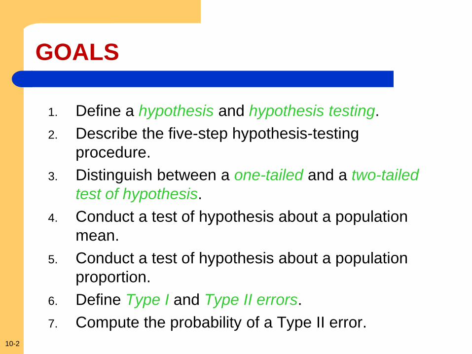
GOALS
1. Define a hypothesis and hypothesis testing.
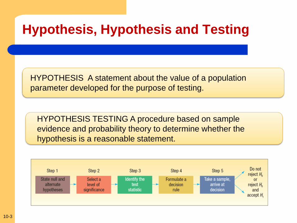
2. Describe the five-step hypothesis-testing
procedure.
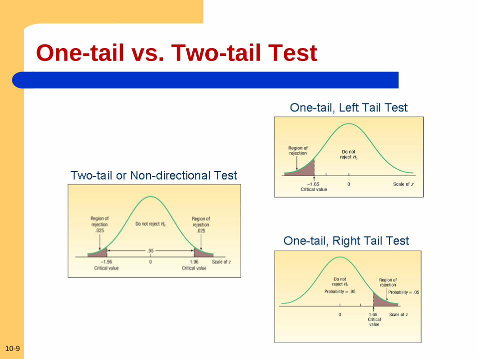
3. Distinguish between a one-tailed and a two-tailed
test of hypothesis.
4. Conduct a test of hypothesis about a population
mean.
5. Conduct a test of hypothesis about a population
proportion.
6. Define Type I and Type II errors.
7. Compute the probability of a Type II error.
10-3
Hypothesis, Hypothesis and Testing
HYPOTHESIS A statement about the value of a population
parameter developed for the purpose of testing.
HYPOTHESIS TESTING A procedure based on sample
evidence and probability theory to determine whether the
hypothesis is a reasonable statement.
10-4
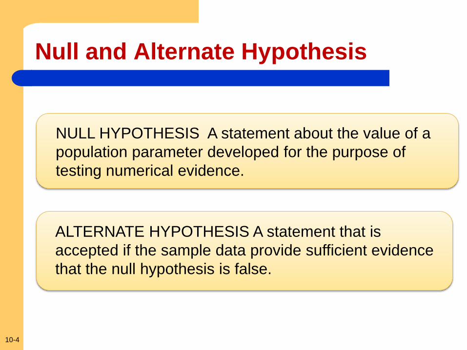
Null and Alternate Hypothesis
NULL HYPOTHESIS A statement about the value of a
population parameter developed for the purpose of
testing numerical evidence.
ALTERNATE HYPOTHESIS A statement that is
accepted if the sample data provide sufficient evidence
that the null hypothesis is false.
10-5
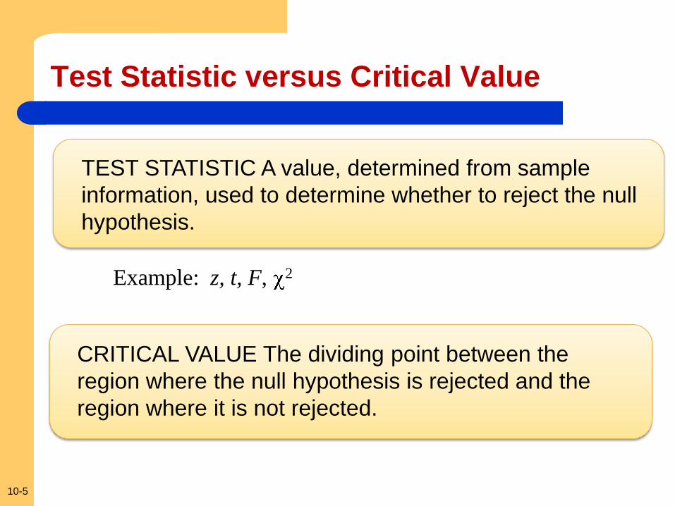
Test Statistic versus Critical Value
TEST STATISTIC A value, determined from sample
information, used to determine whether to reject the null
hypothesis.
CRITICAL VALUE The dividing point between the
region where the null hypothesis is rejected and the
region where it is not rejected.
Example: z, t, F, 2
10-6
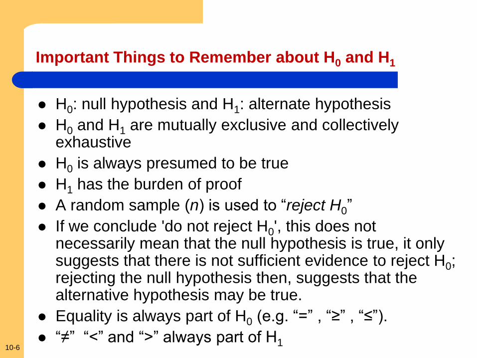
Important Things to Remember about H0 and H1
H0: null hypothesis and H1: alternate hypothesis
H0 and H1 are mutually exclusive and collectively exhaustive
H0 is always presumed to be true
H1 has the burden of proof
A random sample (n) is used to “reject H0”
If we conclude 'do not reject H0', this does not necessarily mean that the null hypothesis is true, it only suggests that there is not sufficient evidence to reject H0; rejecting the null hypothesis then, suggests that the alternative hypothesis may be true.
Equality is always part of H0 (e.g. “=” , “≥” , “≤”).
“≠” “<” and “>” always part of H1
10-7
How to Set Up a Claim as Hypothesis
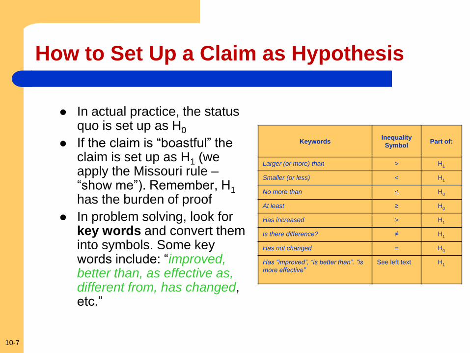
In actual practice, the status quo is set up as H0
If the claim is “boastful” the claim is set up as H1 (we apply the Missouri rule – “show me”). Remember, H1 has the burden of proof
In problem solving, look for key words and convert them into symbols. Some key words include: “improved, better than, as effective as, different from, has changed, etc.”
Keywords Inequality
Symbol Part of:
Larger (or more) than > H1
Smaller (or less) < H1
No more than H0
At least ≥ H0
Has increased > H1
Is there difference? ≠ H1
Has not changed = H0
Has “improved”, “is better than”. “is
more effective”
See left text H1
10-8
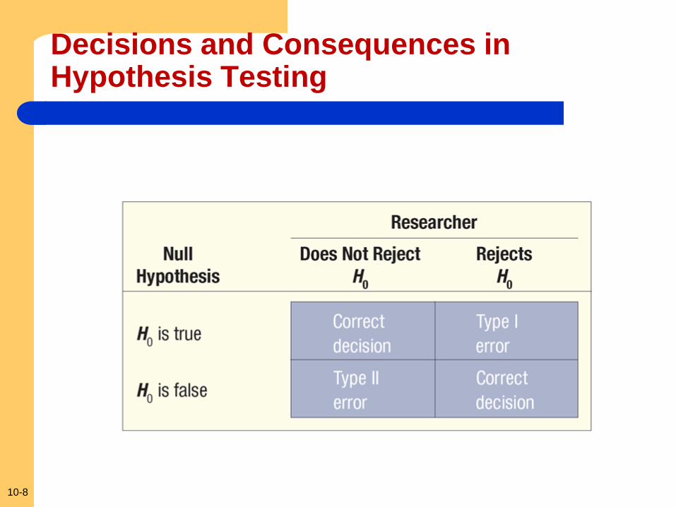
Decisions and Consequences in Hypothesis Testing
10-9
One-tail vs. Two-tail Test
10-10
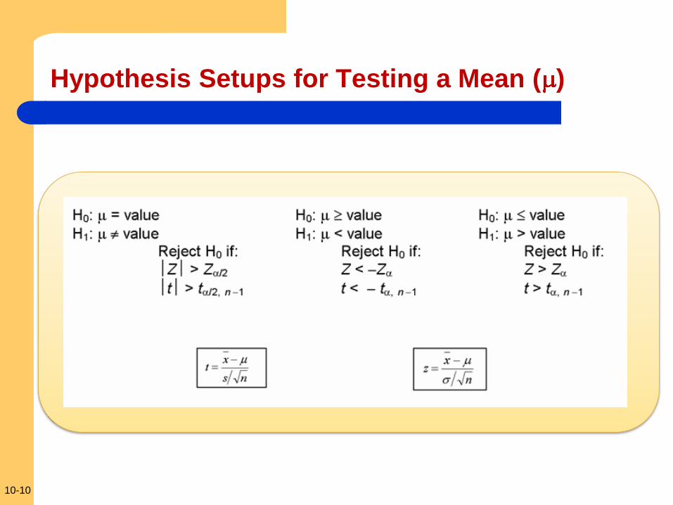
Hypothesis Setups for Testing a Mean ( )
10-11
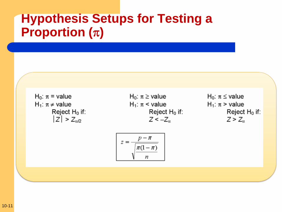
Hypothesis Setups for Testing a Proportion ( )
10-12
Testing for a Population Mean with a Known Population Standard Deviation- Example
Jamestown Steel Company manufactures and assembles desks and other office equipment . The weekly production of the Model A325 desk at the Fredonia Plant follows the normal probability distribution with a mean of 200 and a standard deviation of 16. Recently, new production methods have been introduced and new employees hired. The VP of manufacturing would like to investigate whether there has been a change in the weekly production of the Model A325 desk.
10-13
Testing for a Population Mean with a Known Population Standard Deviation- Example
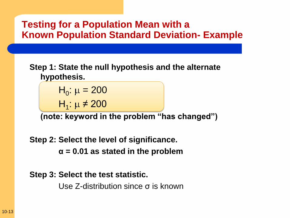
Step 1: State the null hypothesis and the alternate
hypothesis.
H0: = 200
H1: ≠ 200
(note: keyword in the problem “has changed”)
Step 2: Select the level of significance.
α = 0.01 as stated in the problem
Step 3: Select the test statistic.
Use Z-distribution since σ is known
10-14
Testing for a Population Mean with a Known Population Standard Deviation- Example
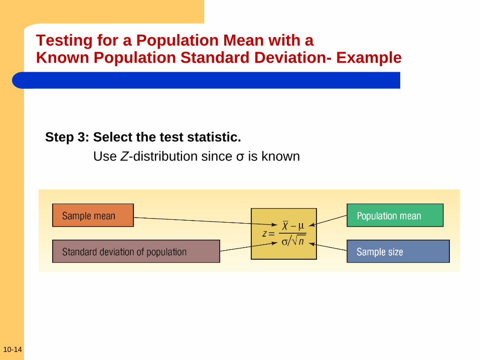
Step 3: Select the test statistic.
Use Z-distribution since σ is known
10-15
Testing for a Population Mean with a Known Population Standard Deviation- Example
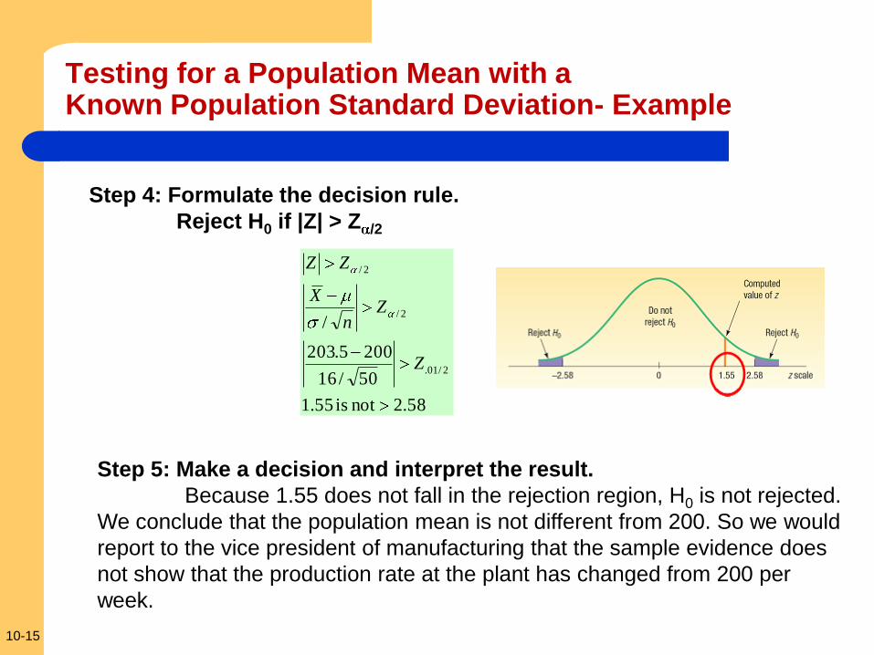
Step 4: Formulate the decision rule.
Reject H0 if |Z| > Z /2
58.2not is 55.1
50/16
2005.203
/
2/01.
2/
2/
Z
Zn
X
ZZ
Step 5: Make a decision and interpret the result.
Because 1.55 does not fall in the rejection region, H0 is not rejected.
We conclude that the population mean is not different from 200. So we would
report to the vice president of manufacturing that the sample evidence does
not show that the production rate at the plant has changed from 200 per
week.
10-16
Suppose in the previous problem the vice
president wants to know whether there has
been an increase in the number of units
assembled. To put it another way, can we
conclude, because of the improved
production methods, that the mean number
of desks assembled in the last 50 weeks was
more than 200?
Recall: σ=16, n=200, α=.01
Testing for a Population Mean with a Known Population Standard Deviation- Another Example
10-17
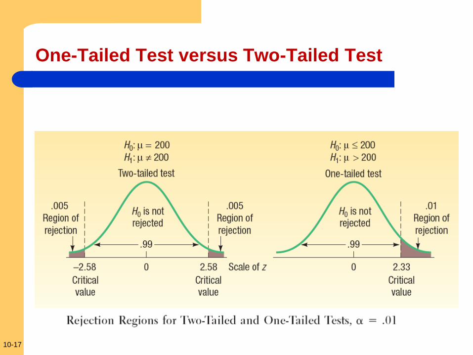
One-Tailed Test versus Two-Tailed Test
10-18
Testing for a Population Mean with a Known Population Standard Deviation- Example
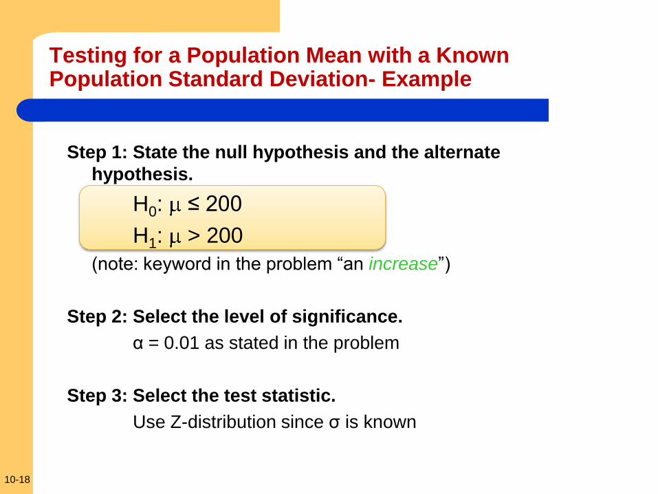
Step 1: State the null hypothesis and the alternate
hypothesis.
H0: ≤ 200
H1: > 200
(note: keyword in the problem “an increase”)
Step 2: Select the level of significance.
α = 0.01 as stated in the problem
Step 3: Select the test statistic.
Use Z-distribution since σ is known
10-19
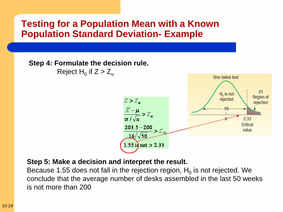
Testing for a Population Mean with a Known Population Standard Deviation- Example
Step 4: Formulate the decision rule.
Reject H0 if Z > Z
Step 5: Make a decision and interpret the result.
Because 1.55 does not fall in the rejection region, H0 is not rejected. We
conclude that the average number of desks assembled in the last 50 weeks
is not more than 200
10-20
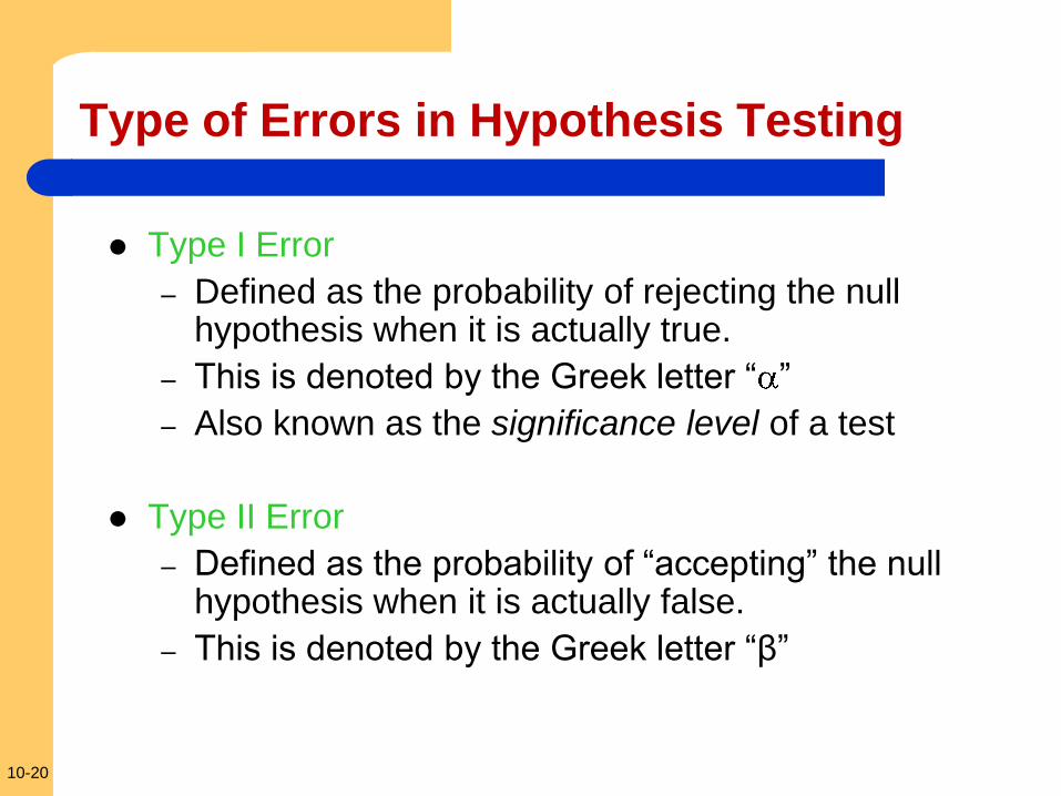
Type of Errors in Hypothesis Testing
Type I Error
– Defined as the probability of rejecting the null hypothesis when it is actually true.
– This is denoted by the Greek letter “ ”
– Also known as the significance level of a test
Type II Error
– Defined as the probability of “accepting” the null hypothesis when it is actually false.
– This is denoted by the Greek letter “β”
10-21
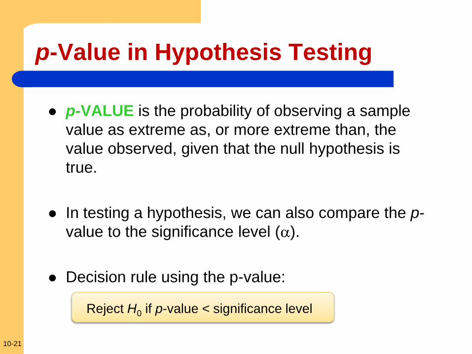
p-Value in Hypothesis Testing
p-VALUE is the probability of observing a sample
value as extreme as, or more extreme than, the
value observed, given that the null hypothesis is
true.
In testing a hypothesis, we can also compare the p-
value to the significance level ( ).
Decision rule using the p-value:
Reject H0 if p-value < significance level
10-22
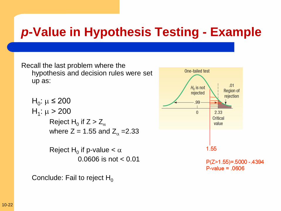
p-Value in Hypothesis Testing - Example
Recall the last problem where the hypothesis and decision rules were set up as:
H0: ≤ 200
H1: > 200
Reject H0 if Z > Z
where Z = 1.55 and Z =2.33
Reject H0 if p-value <
0.0606 is not < 0.01
Conclude: Fail to reject H0
10-23
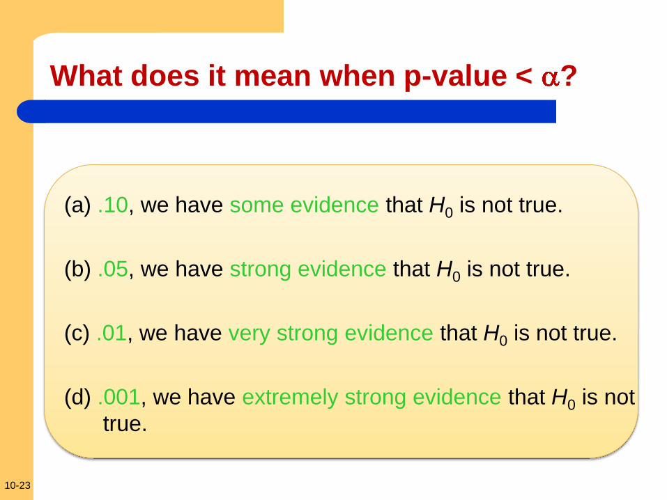
What does it mean when p-value < ?
(a) .10, we have some evidence that H0 is not true.
(b) .05, we have strong evidence that H0 is not true.
(c) .01, we have very strong evidence that H0 is not true.
(d) .001, we have extremely strong evidence that H0 is not
true.
10-24
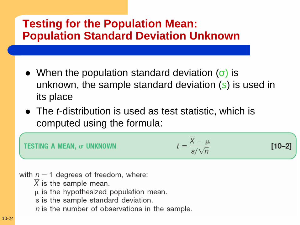
Testing for the Population Mean: Population Standard Deviation Unknown
When the population standard deviation (σ) is
unknown, the sample standard deviation (s) is used in
its place
The t-distribution is used as test statistic, which is
computed using the formula:
10-25
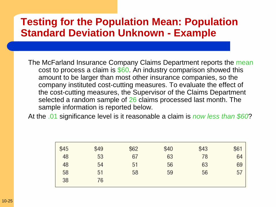
Testing for the Population Mean: Population Standard Deviation Unknown - Example
The McFarland Insurance Company Claims Department reports the mean cost to process a claim is $60. An industry comparison showed this amount to be larger than most other insurance companies, so the company instituted cost-cutting measures. To evaluate the effect of the cost-cutting measures, the Supervisor of the Claims Department selected a random sample of 26 claims processed last month. The sample information is reported below.
At the .01 significance level is it reasonable a claim is now less than $60?
10-26
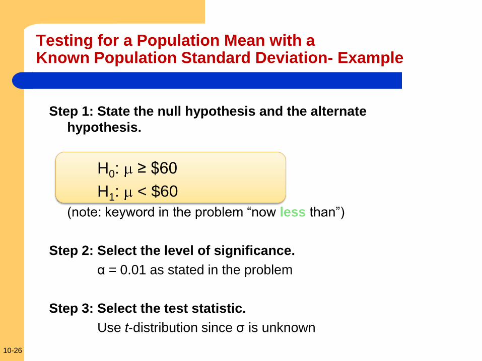
Testing for a Population Mean with a Known Population Standard Deviation- Example
Step 1: State the null hypothesis and the alternate
hypothesis.
H0: ≥ $60
H1: < $60
(note: keyword in the problem “now less than”)
Step 2: Select the level of significance.
α = 0.01 as stated in the problem
Step 3: Select the test statistic.
Use t-distribution since σ is unknown
10-27
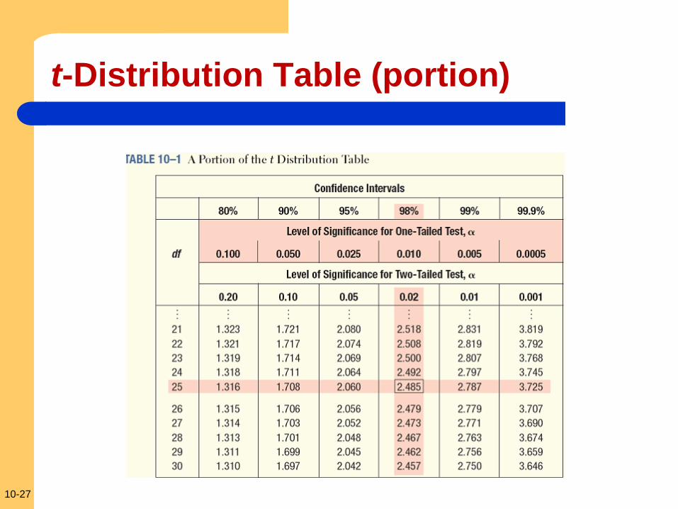
t-Distribution Table (portion)
10-28
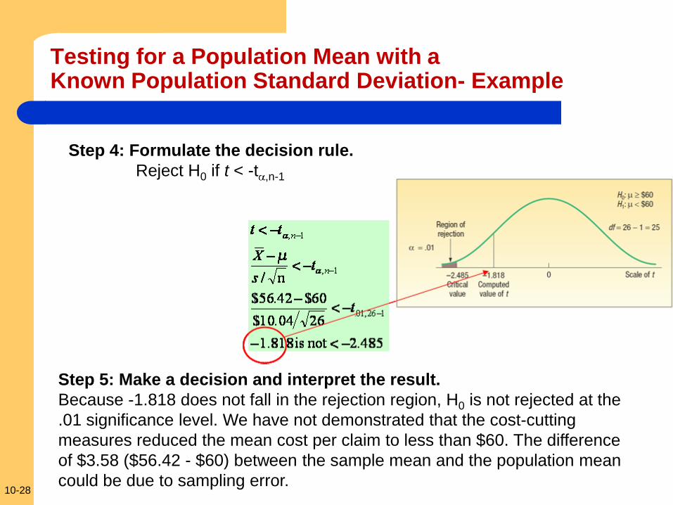
Testing for a Population Mean with a Known Population Standard Deviation- Example
Step 5: Make a decision and interpret the result.
Because -1.818 does not fall in the rejection region, H0 is not rejected at the
.01 significance level. We have not demonstrated that the cost-cutting
measures reduced the mean cost per claim to less than $60. The difference
of $3.58 ($56.42 - $60) between the sample mean and the population mean
could be due to sampling error.
Step 4: Formulate the decision rule.
Reject H0 if t < -t ,n-1
10-29
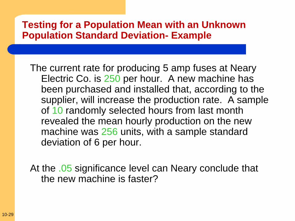
The current rate for producing 5 amp fuses at Neary Electric Co. is 250 per hour. A new machine has been purchased and installed that, according to the supplier, will increase the production rate. A sample of 10 randomly selected hours from last month revealed the mean hourly production on the new machine was 256 units, with a sample standard deviation of 6 per hour.
At the .05 significance level can Neary conclude that the new machine is faster?
Testing for a Population Mean with an Unknown Population Standard Deviation- Example
10-30
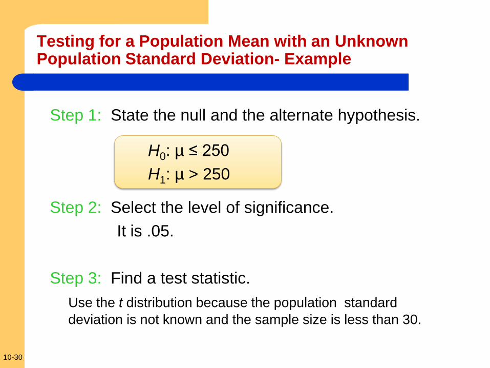
Step 1: State the null and the alternate hypothesis.
H0: µ ≤ 250
H1: µ > 250
Step 2: Select the level of significance.
It is .05.
Step 3: Find a test statistic.
Use the t distribution because the population standard
deviation is not known and the sample size is less than 30.
Testing for a Population Mean with an Unknown Population Standard Deviation- Example
10-31
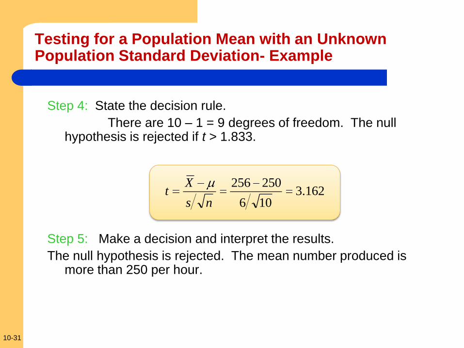
Step 4: State the decision rule.
There are 10 – 1 = 9 degrees of freedom. The null hypothesis is rejected if t > 1.833.
Step 5: Make a decision and interpret the results.
The null hypothesis is rejected. The mean number produced is more than 250 per hour.
162.3106
250256
ns
Xt
Testing for a Population Mean with an Unknown Population Standard Deviation- Example
10-32
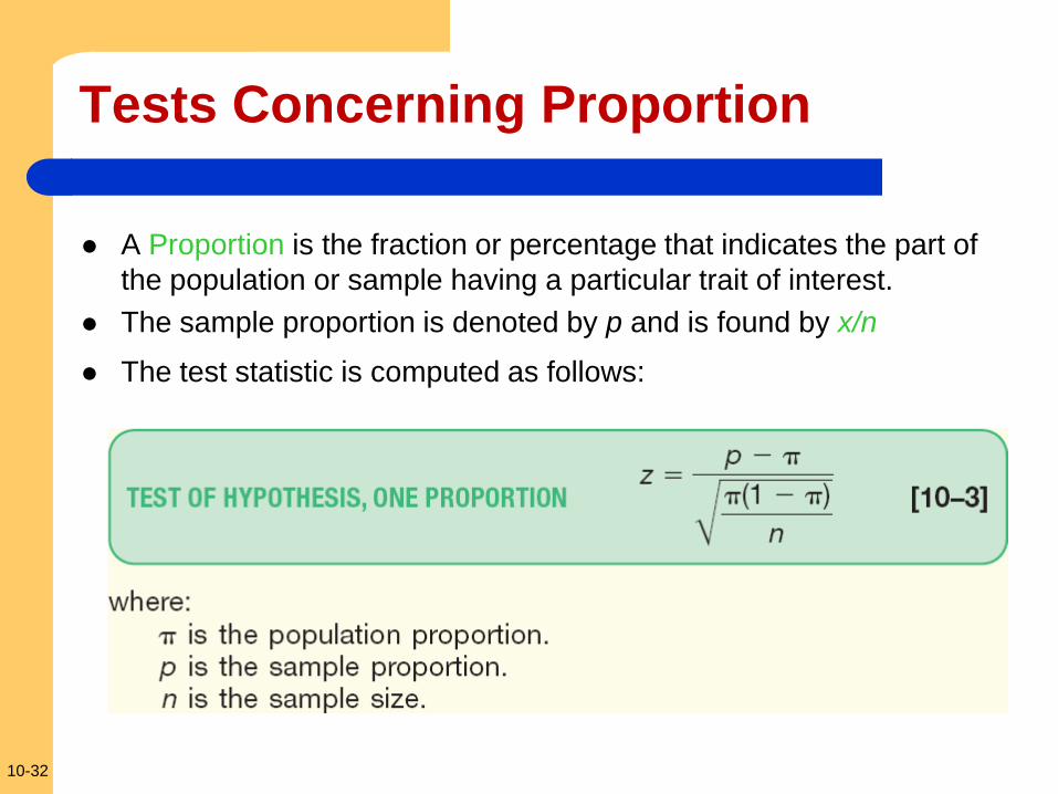
Tests Concerning Proportion
A Proportion is the fraction or percentage that indicates the part of
the population or sample having a particular trait of interest.
The sample proportion is denoted by p and is found by x/n
The test statistic is computed as follows:
10-33
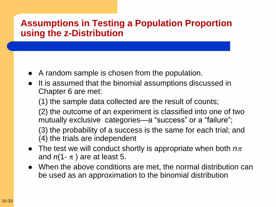
Assumptions in Testing a Population Proportion using the z-Distribution
A random sample is chosen from the population.
It is assumed that the binomial assumptions discussed in Chapter 6 are met:
(1) the sample data collected are the result of counts;
(2) the outcome of an experiment is classified into one of two mutually exclusive categories—a “success” or a “failure”;
(3) the probability of a success is the same for each trial; and (4) the trials are independent
The test we will conduct shortly is appropriate when both n and n(1- ) are at least 5.
When the above conditions are met, the normal distribution can be used as an approximation to the binomial distribution

10-34
Test Statistic for Testing a Single Population Proportion
n
pz
)1(
Sample proportion
Hypothesized
population proportion
Sample size
10-35
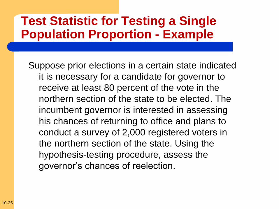
Test Statistic for Testing a Single Population Proportion - Example
Suppose prior elections in a certain state indicated
it is necessary for a candidate for governor to
receive at least 80 percent of the vote in the
northern section of the state to be elected. The
incumbent governor is interested in assessing
his chances of returning to office and plans to
conduct a survey of 2,000 registered voters in
the northern section of the state. Using the
hypothesis-testing procedure, assess the
governor’s chances of reelection.
10-36
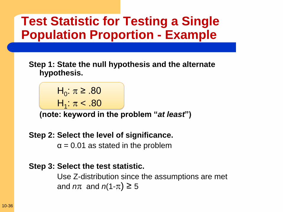
Test Statistic for Testing a Single Population Proportion - Example
Step 1: State the null hypothesis and the alternate hypothesis.
H0: ≥ .80
H1: < .80 (note: keyword in the problem “at least”)
Step 2: Select the level of significance.
α = 0.01 as stated in the problem
Step 3: Select the test statistic.
Use Z-distribution since the assumptions are met
and n and n(1- ) ≥ 5
10-37
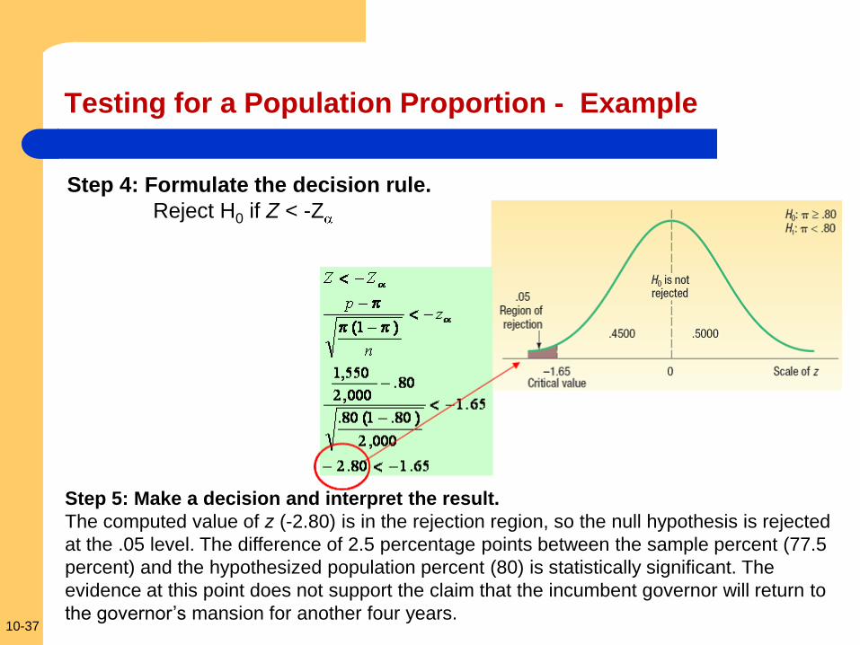
Testing for a Population Proportion - Example
Step 5: Make a decision and interpret the result.
The computed value of z (-2.80) is in the rejection region, so the null hypothesis is rejected
at the .05 level. The difference of 2.5 percentage points between the sample percent (77.5
percent) and the hypothesized population percent (80) is statistically significant. The
evidence at this point does not support the claim that the incumbent governor will return to
the governor’s mansion for another four years.
Step 4: Formulate the decision rule.
Reject H0 if Z < -Z
10-38
Type II Error
Recall Type I Error, the level of significance, denoted by the Greek letter “ ”, is defined as the probability of rejecting the null hypothesis when it is actually true.
Type II Error, denoted by the Greek letter “β”,is
defined as the probability of “accepting” the null hypothesis when it is actually false.
10-39
Type II Error - Example
A manufacturer purchases steel bars to make cotter
pins. Past experience indicates that the mean tensile
strength of all incoming shipments is 10,000 psi and
that the standard deviation, σ, is 400 psi. In order to
make a decision about incoming shipments of steel
bars, the manufacturer set up this rule for the quality-
control inspector to follow: “Take a sample of 100
steel bars. At the .05 significance level if the sample
mean strength falls between 9,922 psi and 10,078
psi, accept the lot. Otherwise the lot is to be
rejected.”
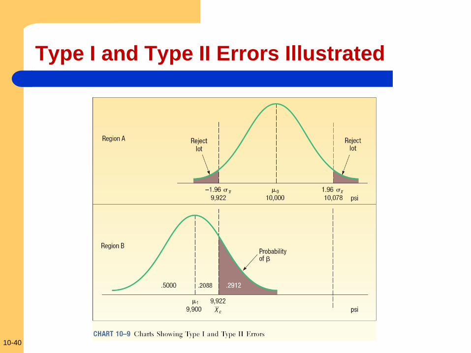
10-40
Type I and Type II Errors Illustrated