One-Machine Scheduling with Unit Jobs and Chain Precedence Relations · Universita degli Studi Roma Tre` Dottorato di Ricerca in Informatica e Automazione XVII Ciclo - 2005 Mara Servilio

Universita degli Studi Roma Tre

Dottorato di Ricerca in Informatica e Automazione

XVII Ciclo – 2005

One-Machine Scheduling with Unit Jobs and Chain

Precedence Relations

Mara Servilio

Universita degli Studi Roma Tre

Dottorato di Ricerca in Informatica e Automazione

XVII Ciclo - 2005

Mara Servilio

One-Machine Scheduling with Unit Jobs and Chain

Precedence Relations

Advisor

Prof. Dario Pacciarelli

Reviewers

Prof. Claudio ArbibProf.ssa Martine Labbe

Author’s address:Mara ServilioDipartimento di Informatica e AutomazioneUniversita degli Studi Roma TreVia della Vasca Navale 79, 00146 Roma, Italye-mail: [email protected], [email protected]: www.di.univaq.it/servilio/hp mara.htm

Contents

Acknowledgements iii

1 Introduction 11.1 A competitive scheduling problem in UMTS

systems . . . . . . . . . . . . . . . . . . . . . . . . . . . . . . . 51.2 A competitive scheduling problem in

Computational Biology . . . . . . . . . . . . . . . . . . . . . . . 101.3 Time-Indexed Formulation of Competitive

Scheduling Problems . . . . . . . . . . . . . . . . . . . . . . . . 13

2 One-machine Scheduling Problem in UMTS Channel Assign-ment 172.1 The problem . . . . . . . . . . . . . . . . . . . . . . . . . . . . 17

2.1.1 Problem formulation . . . . . . . . . . . . . . . . . . . . 172.1.2 Problem complexity . . . . . . . . . . . . . . . . . . . . 19

2.2 Solution algorithms . . . . . . . . . . . . . . . . . . . . . . . . . 212.2.1 A dynamic programming algorithm for β-FCFS . . . . . 212.2.2 A fast lagrangian heuristic for β-FCFS and M-FCFS . . 222.2.3 An iterative greedy-like heuristic . . . . . . . . . . . . . 28

2.3 Computational experience . . . . . . . . . . . . . . . . . . . . . 29

3 Polyhedral study of one-machine scheduling problem: the caseof a single user 333.1 Introduction . . . . . . . . . . . . . . . . . . . . . . . . . . . . . 333.2 PSP1 . . . . . . . . . . . . . . . . . . . . . . . . . . . . . . . . . 383.3 CSP1 . . . . . . . . . . . . . . . . . . . . . . . . . . . . . . . . . 46

4 Polyhedral study of one-machine scheduling problem: the caseof two users 494.1 PSP2 . . . . . . . . . . . . . . . . . . . . . . . . . . . . . . . . . 494.2 SP2 . . . . . . . . . . . . . . . . . . . . . . . . . . . . . . . . . 784.3 CSP2 . . . . . . . . . . . . . . . . . . . . . . . . . . . . . . . . . 79

i

ii CONTENTS

5 Conclusions 87

Acknowledgements

There are many people which supported my activity in the last three yearsand I want to spend few words of thanks for them.First of all, I wish to thank my tutor Claudio Arbib for passing me his enthu-siasm for the research. I thank him for all precious comments and advice, forhis encouragement and support, and for indispensable help in the realizationof this work. I’m also grateful to Martine Labbe for giving me the opportunityto spend four pleasant months in Bruxelles. I learned a lot from her and aconsiderable part of this thesis is due to her contribution. I thank my advisorDario Pacciarelli and Professor Fernando Nicolo for their help, especially inthe first months of my doctoral course: they made for my complete integrationwith the research group of the University of Rome. My special thanks are dueto Gaia Nicosia, Fabrizio Rossi and Stefano Smriglio for their friendship andhelpfulness in answering to all my questions. They have been a very importantguide for me!

There are several other people I’m grateful to: Monia, Fabrizio and Sal-vatore for useful suggestions during our discussions on various topics; all thePhD students of L’Aquila, for making pleasant these three years; Marta, Lu-dovica and Alessandra, for our continuous scientific exchanges and for theirmoral support before I gave my talks. They are great friends for me!

Finally, I want to thank my family for having total trust in all my choice,and Fabio for his infinite patience and love.

Rome, April 30, 2005 Mara Servilio

iii

iv ACKNOWLEDGEMENTS

Chapter 1

Introduction

The scheduling problems arise whenever one has to allocate resources to acti-vities over time. Originally, these problems were solved by general mathema-tical programming tools (linear programming, flows) but, in the seventies, thedevelopment of the computational complexity theory allowed to solve schedu-ling problems in a systematic way, by studying their complexity, some resolu-tive solution algorithms and their applications in to real life.In general, when defining a scheduling problem one specifies the features ofthe system (i.e. the available resources), of the jobs (i.e. the activities whichhave to be performed) and of the objectives that one wants to optimize.Most classical papers on scheduling relate to deterministic, off-line models,and are based on particular assumptions which are not always compatiblewith the real features of the problem; that explains why, in the last few years,it was begun to consider on-line and stochastic scheduling models taking intoaccount the real aspects of the problem.In a classical approach, the jobs belong to a single user which wants to orga-nize and exploit the available resources in the most useful way: in particularthere is a single objective function which has to be optimized. Also in thecase in which there are more objectives, the resolutive solution algorithms aredesigned in a perspective in which a single decision-maker seeks for an optimalschedule of the system.A very different situation is when there are more agents, each with its own setof jobs, in competition for the same resources and there is no “authority” ableto solve possible conflicts among them. In this case, it is necessary to redefine,at least in part, the model so as to offer the possibility of a negotiation amongthe agents in such way that they can obtain a resource allocation admissible.Many disciplines such as Combinatorial Optimization, Game Theory , Ar-tificial Intelligence and Decision Theory provide an approach to multi-agentscheduling problems; in fact, the study of these models has been frequently

1

2 1 Introduction

motivated by the real requirements in different fields. For example, in [3] theAuthors consider the problem in which two different railway societies have tonegotiate the use of a common track. Each society has a set of trains and afixed timetable to respect: the objective of each agent consists in minimizingthe sum of the delay for his own trains.

In multi-agent scheduling models, a fundamental difference arises depen-ding on whether it is possible to transfer utilities among the agents or not;this condition tipically means that all the users which are penalized from acertain allocation can be balanced by money.In this work, we consider the case in which the transfer is not allowed andanalyze a particular class of Combinatorial Otpimization problems known asCompetitive Scheduling problems. In particular, we will discuss more in detailthe situation when two users compete for the same single resource. Approa-ching such problem, we can adopt two slightly different viewpoints: we canoptimize the performance of one user by according to the other an utility atleast equal to a reasonable fixed threshold, or we can determine the set ofall the nondominated schedules, i.e. such that a better schedule for one usernecessarily corresponds to a worse schedule for the other. Since we consider asingle shared resource, the problem is analougous to a single-machine competi-tive scheduling problem. Observe that for competitive scheduling problems weconsider again a single decision-maker, unlike most of multi-agent schedulingproblems.

We introduce the general notation for Competitive Scheduling.Let N be the set of agents, each of them having a set of nonpreemptive jobsto process; for each agent i ∈ N , we denote J i its own set of jobs and J i

j

its own j-th job whose processing time is indicated with pij . Let ni = |J i|;

depending on the situation, each job can be associated with other parametersas a due-date di

j (i.e. the time by which the job j should be completed), arelease date ri

j (i.e. the time before which the job j cannot start processing),a weight wi

j (i.e. the profit/cost for each time unit in which the job j is inprogress). A general schedule σ is an assignment of starting times to eachjob and Ci

j(σ) denotes the completion time of job J ij in the schedule σ. Each

agent i is associated with an utility function f i(σ) which is non-decreasingwhen the completion times increase and the objective of each user consistsin maximizing its own utility function. In certain cases, this function can bereplaced with a cost function and then the objective becomes to minimize it.When necessary, we will use the classical three-field notation for the schedu-ling problems α|β|γ, where α identifies the system and the number of machinesand contains a single entry, β provides the (possible) particular features of thesystem and may contain no entries, a single entry or multiple entries, and γ

identifies the objective function and usually contains a single entry.

3

Possible machine environments specified in the α field are

• Single machine (α = 1);

• Identical machines in parallel (α = Pm);

• Machines in parallel with different speeds (α = Qm);

• Flow shop (α = Fm): there are m machines in series and each job has tobe processed on each one of the m machines. All the job have the samerouting for the processing;

• Job shop (α = Jm): there is the same situation as the flow shop, buteach job has its own route to follow for the processing.

Possible entries in the β field are

• Release dates (β = rj);

• Preemptions (β =prmp): preemptions imply that it is not necessary tokeep a job on a machine until completion;

• Precedence constraints (β = prec);

• Breakdowns (β =brkdwn): breakdowns imply that machines are notcontinuously available.

Finally, possible objective functions specified in the γ field are

• Makespan (γ = Cmax): the makespan is equivalent to the completiontime of the last job to leave the system;

• Total weighted completion time (γ =∑

j wjCj);

• Total weighted tardiness (γ =∑

j wjTj): the tardiness is defined asTj = max{Cj − dj , 0}, where Cj is the completion time of job j and dj

is its due-date;

• Weighted number of tardy jobs (γ =∑

j wjUj).

In the literature, very important contributions regarding Competitive Sche-duling have been recently provided by [1] and [2]. In [1], the Authors considerthe scenario where two users compete to perform their respective jobs on acommon set of resources: they describe the set of nondominated schedules forwhich the users may negotiate and develop a polynomial algorithm to find thisnondominated set. In [2], the same Authors consider the problem of schedu-ling general length jobs with no-precedence relations on a single machine, with

4 1 Introduction

the objective of best compromising between two regular functions of the jobcompletion times. They characterize the complexity of decision problems ari-sing for different combinations of the objective functions for the two users anddifferent system structures and, for some special cases, they enumerate all thenondominated solutions.A similar argument has been approached in [4], where the Authors analyzea one-machine scheduling problem in which two or more agents are involvedand assume that, unlike most scheduling problems, each agent has its ownobjective. This is not the case of traditional models, in which different jobsrepresent different users but individual requirements of each user do not affectthe scheduling criterion. Instead, in [4] the model is characterized by multi-ple scheduling criteria and different objectives each of them associated witha class of agents. In other words, each agent self-selects according to its ownpreferred criterion and the objective consists in optimizing a weighted averageof the criteria. In this work, three main criteria are considered: minimizingmakespan, minimizing maximum lateness and minimizing total weighted com-pletion time and it is proved that, unlike the case in which only one of thesecriteria is considered, when a mix of them is minimized the problem becomesNP-hard. Further, some dominance properties which hold for the problemhave been provided.

On the other hand, we mention that multi-agent scheduling problems havebeen extensively studied by [13] and [16] in the manufacturing systems; in thisarea, all the elements of the manufacturing process (machines, jobs, workers...)can play the role of agents, each of them having the aim to maximize its ownproductivity.In [20] a decentralized scheduling problem is considered; it consists in allocat-ing resources for distributed computing systems whose nature of computationcan be decentralized. For example, think to a problem of scheduling networkaccess for programs representing different users on the internet scenario: allthe modules of the system represent independent users, each of them havingcompeting requirements and localized informations about their needs.The independence among the users can be managed by treating the modulesas agents which have the autonomy to decide how exploit their resources andwhich can communicate each other, by messages, some of their private in-formations. A decentralized solution is to manage message passing, to reachclosure and to realize the final schedule. These problems can be solved bymarket mechanisms; in [20], the Authors show how some results in economictheory can be applied to decentralized scheduling, describe a specific problemof this kind and provide a formal economic model of it.

This research was motivated by two main applications.The first concerns a two-users competitive scheduling problem arose in a Uni-

1.1. A COMPETITIVE SCHEDULING PROBLEM IN UMTS

SYSTEMS 5

versal Mobile Telecommunication System (UMTS) developed within the Euro-pean IST project FUTURE [6]. The project contributes to the specication ofthe 3rd generation mobile communication system developed by the EuropeanTelecommunications Standard Institute. In particular, it aims at adopting therecent advances of the internet scene in UMTS by exploring the applicabilityof native internet protocols in 3G, and investigating and developing enhancedQuality of Service (QoS) strategies for a packet based UMTS.We consider the procedures in charge of assigning the channel capacity to themobile terminals (users). These procedures are part of the scheduling functionimplemented in downlink by the system. Since the system includes two users,a competitive scheduling problem arises in which one wants to maximize or theon-time packets transmitted to one user while guaranteeing certain amountsof on-time packets to the other, or the total on-time traffic for each user, orthe worst between the total on-time traffic of the two users.

The second application concerns an alignment problem in ComputationalBiology, where the main objective is to compare two (or more) biological ob-jects which consist of a set of elements arranged in a linearly ordered structureand to align them by determining subsets of corresponding elements in each.Typical examples are the alignments of genomic sequences or proteins.

1.1 A competitive scheduling problem in UMTS

systems

The introduction of UMTS telecommunication systems is a very innovativeevent which allows to reach a lot of objectives such that the convergencebetween fixed and mobile networks and the availability of a large range of ser-vices called “multimedia communication”. The main functionality of UMTSnetworks is the capacity to support wideband service data, symmetric andasymettric communications, real-time and non-real-time services and packetswitched traffic which allows to simultaneously transmit data with differentbit-rates.

Since a UMTS system satisfies a lot of services having very different fea-tures, it is essential that the network associates each of them with a certainQuality of Service which allows to univocally identify the requirements of thetransport service that one can use.In a UMTS system it is possible to distinguish four different QoS classes:

• Conversational Class: the main services provided by this class are thecommunications among two or more users. Then, it is used to transmitreal-time data and is very susceptible to the transfer time; in particular,for this class a very short transfer delay is tolerated since the qualityrequirements are determined by the human perceptions.

6 1 Introduction

• Streaming Class: it is used to transmit real-time data both video andaudio kinds and it allows a transfer delay greater than the conversationalclass.

• Interactive Class: the typical services satisfied by this class are the webbrowsing, the research in a database and the access to a certain server.Then, the main requirements of the interactive class are a reasonabletransfer delay and a transparent data transmission having a minimumerror rate.

• Background Class: it is used to satisfy services such as e-mail and SMStransfer or files download. Since they do not belong to a real-time traffic,this class is not as suscetible to the transfer delay as the others, but itrequires a maximum reliability and integrality of the data transmission.

A UMTS system operates via protocols associated with distinct layers, sothat the communication within a layer is transparent with respect to all thelower level layers. The UMTS radio interface is made up of three main layers:

• Physical Layer (L1)

• Data Link Layer (L2)

• Network Layer (L3)

In particular, in the layer L2 we distinguish further sub-levels as MediumAccess Control (MAC), Radio Link Control (RLC), Packet Data ConvergenceProtocol (PDCP) and Broadcast/Multicast Control (BMC).The physical layer (PHY) is the lowest layer in the ISO/OSI reference modeland it supports all the functionalities allowing the transmission on the physicalstratum; in particular, it provides the transfer of the useful traffic to MAC andall the higher levels.

In this work, we consider the communication from MAC module to physi-cal layer. We distinguish between the downlink and the uplink communicationdepending on wheter a message is transmitted from MAC to physical layer atgateway side or at user side, respectively.The data transfer between MAC and PHY protocols occurs via transportchannels which are associated with a transport format, i.e. an appropriatecombination of scrambling, interleaving and bit rate to apply to each informa-tion which has to be transmitted.

We focus on the communication from gateway to user (in the following, thedownlink communication) at the gateway side (white arrow in Figure 1.1a);the data are transmitted by a unique transport channel, named Downlink


SYSTEMS 7

Shared CHannel (DSCH). In the FUTURE demonstrator, the message formatrelevant to this communication is the one reported in Figure 1.1b.

Figure 1.1: a) layers involved and b) message format in the downlink communicationbetween MAC and PHY.

The useful traffic information is contained in the DSCH section of the message.According to the traffic load, the length of this section can be 5120, 2560 or0 bits. Every Trasmission Time Interval (TTI, corresponding to 40 msec) a

8 1 Introduction

message exchange occurs between the MAC and the PHY protocols, see Figure1.1a, yielding a bit rate of 128, 64 or 0 Kbit/sec depending on the differentlength of the DSCH sections. For further details, see [5].

A relevant issue in FUTURE is that, unlike previous projects on the samesubject, different services and applications can simultaneously be provided totwo mobile users (say A and B) by a unique physical channel per satellitebeam. Since the services may have different QoS requirements, a need arisesto coordinate the radio resource utilization. Such a need is particularly de-manding in downlink because in this case the DSCH can be accessed by bothmobile terminals, and not only has the scheduler to select suitable transportformats to maximize the ratio between useful traffic and signalling, but alsohas to specify how the channel is to be shared. Since multiplexing is performedusing orthogonal variable spreading factor codes, the DSCH capacity can beassigned in four ways only: either the channel is completely dedicated to oneuser, or completely dedicated to the other, or equally divided between the two,or finally not assigned. Note that the access mode to the DSCH (at most twousers per TTI) can be applied to an arbitrary number of active users: far frombeing a limit, this practice avoids an excessive packet segmentation and thederived overhead.

Deciding at each TTI how to assign the DSCH capacity to users is thetask of a module called Capacity Planner. Figure 1.2 illustrates the inte-ractions between the Capacity Planner and the other modules of the FUTUREscheduling function, in particular the Short-term Scheduler which is in chargeof packet segmentation and of selecting the most suitable transport format forthe communication.


SYSTEMS 9

Figure 1.2: System architecture: interactions between the Capacity Planner andother modules.

10 1 Introduction

Packets are stored in two groups of 13 queues (logical channel) each.A group corresponds to a user and a logical channel to a specific applica-tion type. For each user, the Capacity Planner constructs blocks of 2560bits(corresponding to half channel capacity, 64Kbit/sec) by selecting packetsfrom the logical channels; then, depending on the traffic, it assigns a numberof blocks between 0 and 2 to each TTI. Each packet is associated with its time-to-leave, that is, with the number of TTIs that may expire before the packetis considered late, and the arrival time of the packet plus the time-to-leavedefines the packet due-date. Once a block is assigned to a TTI, the numberof on-time packets (or the total number of on-time bits) is completely deter-mined. Since this measure can be associated with every pair (block, TTI),computing an optimum plan means finding an assignment of blocks to TTIswhich maximizes the on-time traffic of the two users. This step involves thesolution of a competitive scheduling problem which is the subject of our study.

Whatever be the algorithm employed by the Capacity Planner to schedulethe channel to the users, it must agree to the following specific implementationrequirement

The order in which data-packets are sent by the transmitter (gateway) mustbe preserved at the receiver (mobile terminal), because no two packets relevantto the same application can be swapped in time.

Since blocks are formed by taking the packets of each application from therelevant queue in their order of arrival, a strict order is defined among theblocks of each user (the blocks of the two users are however ranked indepen-dently on each other). Then, by the above requirement any feasible scheduleof blocks to TTIs must fulfill two conditions:

No-cross Condition. The input and output orders are to be consistent: if blocki is assigned to the s-th TTI of the planning horizon, block j to the t-th, andi precedes j, then necessarily s < t.

No-loss Condition. No block is to be lost: if block i is assigned to the s-th TTIof the planning horizon, block j to the t-th, and there is a block k betweeni and j, then k must necessarily be assigned to some TTI (between the s-thand the t-th).

In this thesis, we will study the combinatorial aspects of the one-machinecompetitive scheduling problem illustrated in this section.

1.2 A competitive scheduling problem in

Computational Biology

Computational Biology expanded greatly in the last years, following the con-

1.2. A COMPETITIVE SCHEDULING PROBLEM IN

COMPUTATIONAL BIOLOGY 11

siderable development of computers which are adopted in several biology labo-ratories to store and manage genomic data; in fact, the use of computers allowsto very quickly complete a lot of projects in this field that otherwise would re-quire long time. One of the most important projects in Computational Biologywas the Human Genome Project which ended in 2001 in the announcement ofthe sequencing of the human genome.

Actually, we distinguish between bioinformatics problems which concernstorage, organitation and distribution of large amounts of genomic data, andComputational Biology which is implemented to solve problems of interpre-tation and analysis of genomic data. In particular, this young science allowsto model biological processes in the cell, to remove experimental errors fromgenomic data, to interpret data and to provide theories regarding their bio-logical interactions.After that biological problem is reformulated in mathematical terms, Com-binatorial Optimization and, particularly, Operations Research is adopted tosolve it, especially in the case in which this problem is NP-hard. Branch-and-Cut, Branch-and-Price and Lagrangian Relaxation are the most adoptedtechniques for Computational Biology problems formulated by Integer Linearor Quadratic Programming.

In this thesis, we study a problem whose a particular case, well-known asAlignment Problem, has been extensively examined in Computational Biology.One can distinguish between sequence and structure alignment problem: theformer constists in comparing more biological objects comprised of elementswhich are arranged in a linearly ordered structure, and in finding a correspon-dence among the elements in each object. This correspondence must preservethe order of elements: this means that, if i-th element in the first object is incorrespondence with j-th element in the second object, then a correspondencebetween an element following i and an element preceding j cannot exist.In mathematical terms, given two biological objects, the former comprisedof n elements and the latter of m, we consider the complete bipartite graphGnm = (V, U, E), where |V | = n, |U | = m and E = V × U . An alignmentcorresponds to a noncrossing matching on Gnm, i.e. a matching in which notwo edges cross.

On the other hand, a typical structure alignment problem in Computa-tional Biology is the Contact Map Overlap (COM) problem, which aims tocompare the structure of different proteins. The proteins are linear chains ofamino acids, or residues, whose type and sequence guarantee a natural distin-ction among them. Each protein folds into a three-dimensional structure and,in this way, it determines its functioning and interaction with other molecules.The comparison among proteins belonging to very different families allows toidentify functional and structural similarity which coulds contain a lot of in-

12 1 Introduction

formations about their common evolution. In order to compare two differentstructures, it is necessary to align them in some way. We observe that se-quence and structure alignments are computationally very different: in fact,the structure alignment is a three-dimensional computational problem and ismore complex than the sequence alignment which is one-dimensional.In general, when a protein folds it may happen that two residues which werenot adjacents in the original sequence, are very close each other in the newspace. The three-dimensional structure of a general protein with n residuesis represented by a contact map, i.e. a 0-1, symmetric, n × n matrix whoseentries equal 1 in correspondence with a pairs of residues which are in con-tact, i.e. that are within a fixed small distance in the protein’s fold, but arenot adjacents in the original sequence. Then, given two folded proteins, theproblem consists in determining an alignment between their residues in orderto establish which among them are equivalents. The aim is to determine thebest alignment in correspondence of which there is the largest set of commoncontacts.In terms of graphs, we consider two undirected graphs G1 = (V, E1) andG2 = (U, E2) and denote a general edge as an ordered pair (i, j). An align-ment of V and U corresponds to a noncrossing matching M on Gnm. If twoedges e = (v1, v2) ∈ E1 and f = (u1, u2) ∈ E2 are such that lines l = {v1, u1}and h = {v2, u2} belong to M , then we say that l and h generate the sharing(e, f). The CMO problem constists in finding an alignment which maximizesthe number of sharings. Exploiting the noncrossing condition for the align-ment problem, it is possible to define the compatibility among sharings. Givenedges e = (v1, v2), e

′= (v

′1, v

′2) ∈ E1 and f = (u1, u2), f

′= (u

′1, u

′2) ∈ E2, we

say that sharings (e, f) and (e′, f

′) are compatible if lines {v1, u1}, {v2, u2},

{v′1, u

′1} and {v′

2, u′2} are noncrossing. At this point, if one defines a new

graph GSC (Sharings Conflict Graph) where each node is associated with apairs {e, f}, for each e ∈ E1 and f ∈ E2, and there exsists an edge betweentwo nodes if and only if the corresponding pairs are not compatible sharings,then the CMO problem can be reduced to a Stable Set problem on GSC . In[11], the Authors provide a rigourous algorithm for structure comparison; inparticular, they develop an effective integer linear programming formulationfor CMO problem and a Branch-and-Cut strategy to solve it; the main inno-vation of this work is the effective use of integer programming method in thefield of biomolecular structure comparison.

1.3. TIME-INDEXED FORMULATION OF COMPETITIVE

SCHEDULING PROBLEMS 13

1.3 Time-Indexed Formulation of Competitive

Scheduling Problems

A lot of scheduling problems are formulated as integer programs by usingtime-indexed variables, i.e. variables indexed by {i, t} where i denotes a joband t a time period in which the job can be processed. In this work, weinvestigate the time-indexed formulation for a nonpreemptive single-machinescheduling problem with precedence constraints and emphasize the competi-tive aspect.

A time-indexed formulation for nonpreemptive single-machine schedulingproblems has been widely studied in [17], where the Authors examine thegeneral problem of choosing jobs over time to allocate on a single machine,taking into account the resource constraints. The time-indexed formulation is

max / min∑

j

∑

t

fj(t)xjt

∑

t

xjt ≤ 1 ∀j

∑

j

∑

s

aj(t − s)xjs ≤ bt ∀t

xjt ∈ {0, 1} ∀j, ∀t

where xjt equal 1 if job j is started in period t and 0 otherwise, fj(t) denotesthe profit/cost associated with the allocation of job j in time t, aj(t − s) isthe amount of resource used by job j after t− s periods and bt is the availableamount of resource in period t.

A special version of this problem is studied in [18], where bt equal 1 foreach period t, pj denotes the processing time of general job j and aj(t − s)equal 1 if 0 ≤ t− s < pj and 0 otherwise. Given a certain time horizon T , thescheduling model is

14 1 Introduction

min∑

j

T−pj+1∑

t=1

fj(t)xjt

T−pj+1∑

t=1

xjt = 1 ∀j

∑

j

t∑

s=t−pj+1

xjs ≤ 1 ∀t ≤ T

xjt ∈ {0, 1} ∀j, ∀t ≤ T − pj + 1

Further special cases can be considered if due-date dj and release date rj areintroduced for each job j; also different objectives, such as weighted start timesor weighted tardiness, can be examined.The first constraint in the above model means that all the jobs in the sy-stem must be assigned to exactly one period in the time horizon; often, thisconstraint makes difficult the study of the problem, especially in a polyhedralapproach. For this reason, in [18] the Authors relax these inequalities bysubstituting them with

T−pj+1∑

t=1

xjt ≤ 1 ∀j

The new constraint means that each job can be assigned to at most one period.Observe that the relaxed time-indexed formulation of this scheduling problemis characterized by set packing constraints.

Frequently, in the real time applications it is necessary to assume thatthe jobs must fulfill some precedence relations among them; in [15], the Au-thors express the fact that job j precedes job k in each feasible schedule byintroducing either the condition

xjt −T−pk+1∑

s=t+pj

xks ≥ 0 ∀t = 1, . . . , T − pj + 1

or the inequality

T−pj+1∑

t=1

(t − 1)xjt + pj −T−pk+1∑

t=1

(t − 1)xkt ≤ 0

Plugging one of them into the original problem, the resulting model is chara-cterized by set packing inequalities plus an add constraint.

1.3. TIME-INDEXED FORMULATION OF COMPETITIVE

SCHEDULING PROBLEMS 15

In this work, we analyze two different competitive scenarios and provide atime-indexed formulation for both of them.

We consider n users competing to assign their own jobs Jk = {1, . . . , nk},k = 1, . . . , n, over time on a common single machine. In the first scenario,we suppose that n = 2 and maximize f1(σ) by guaranteeing that the valuef2(σ) ≥ b, where b is a fixed non-negative threshold (if we minimize theobjective function, then f2(σ) ≤ b). For each job j ∈ Jk , k = 1, 2, we define aprocessing time pk

j and a profit/cost fkj (t) associated with the assignment of

job j ∈ Jk to period t. If we assume that not all the jobs must be assigned (i.e.an optimal schedule may not be complete), then the time-indexed formulationof the problem is

max∑

j∈J1

T−p1j+1∑

t=1

f1j (t)xjt

∑

j∈J2

T−p2j+1∑

t=1

f2j (t)yjt ≥ b

T−p1j+1∑

t=1

xjt ≤ 1 ∀j ∈ J1

T−p2j+1∑

t=1

yjt ≤ 1 ∀j ∈ J2

∑

j∈J1

t∑

s=t−p1j+1

xjs ≤ 1 ∀t = 1, . . . , T

∑

j∈J2

t∑

s=t−p2j+1

yjs ≤ 1 ∀t = 1, . . . , T

xjt ∈ {0, 1} ∀j ∈ J1, ∀t ≤ T − p1j + 1

yjt ∈ {0, 1} ∀j ∈ J2, ∀t ≤ T − p2j + 1

where xjt and yjt are the variables associated with user 1 and 2, respectively.Also this model is characterized by set packing inequalities plus an add con-straint (the first, in the above formulation) which is, in this case, a knapsackconstraint.

In the second scenario, we solve the scheduling problem by maximizing/minimizingthe amount f1(σ)+f2(σ). Then, the knapsack constraint disappears from thetime-indexed formulation, the objective function is modified and the model isdescribed by set packing constraints, only.

16 1 Introduction

Then, the correspondence between time-indexed one-machine scheduling(1S) and set packing (SP) formulations is as follows

1S ⇔ SP1S + prec ⇔ SP + add constraint1S + prec + competitive relations ⇔ SP + knapsack constraint

In this thesis, unlike in [18] and [15] we will study both the competitiveversions of the one-machine scheduling problem above introduced. Moreover,we will assume that each job has a unit processing time and include chain-like precedence constraints; in [15], the Authors studied the non-competitiveversion with general processing times and general precedence relations, butfor the special model whose formulation is in terms of completion times.

The work is divided into two fundamental parts. In the former (Chapter 2),we will study the complexity of the first scenario of the competitive schedulingproblem and present different resolutive approachs to solve it and its particu-lar cases, also taking into account the real-time constraints originated by theapplications. In the latter (Chapters 3, 4), we will propose a polyhedral studyof the second scenario of the problem. In particular, after that different caseshave been listed, we examine the dimension of the polyhedron defined as theconvex hull of feasible assignments of each problem and determine some facet-defining inequalities for it.

Chapter 2

One-machine SchedulingProblem in UMTS ChannelAssignment

In this chapter we formulate and discuss the competitive scheduling problemsolved by the Capacity Planner in the UMTS application, as described in §1.1.

2.1 The problem

In §2.1.1 two general formulations of the problem are specialized through pro-perties of objectives and solutions inherited by the application. In §2.1.2 thecomplexity of the resulting problems is investigated.

2.1.1 Problem formulation

Let A, B be disjoint sets of n1, n2 jobs with unit processing times and T bea set of m unit time slots. In our application,

• each set of jobs corresponds to a distinct user (A or B);

• a job corresponds to a block of segmented data-packets: packets in ablock may belong to different applications activated by the relevant user,and may have different due dates;

• each time slot corresponds to half TTI (20 ms).

From now on we will assume that a strict order is defined between the elementsof A (of B, of T ).

The function σ : A ∪ B → T represents a competitive schedule whichassigns a set of jobs to a set of slots. In a feasible schedule not all the jobs (the

17

18 2 One-machine Scheduling Problem in UMTS Channel Assignment

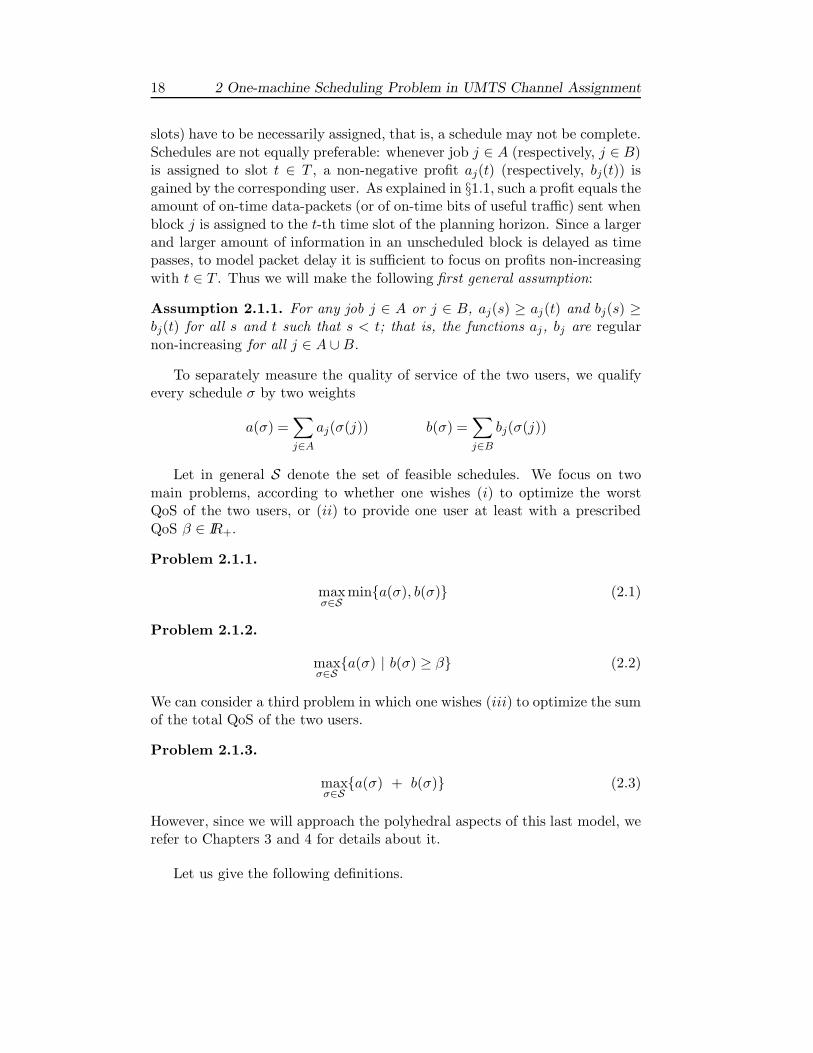
slots) have to be necessarily assigned, that is, a schedule may not be complete.Schedules are not equally preferable: whenever job j ∈ A (respectively, j ∈ B)is assigned to slot t ∈ T , a non-negative profit aj(t) (respectively, bj(t)) isgained by the corresponding user. As explained in §1.1, such a profit equals theamount of on-time data-packets (or of on-time bits of useful traffic) sent whenblock j is assigned to the t-th time slot of the planning horizon. Since a largerand larger amount of information in an unscheduled block is delayed as timepasses, to model packet delay it is sufficient to focus on profits non-increasingwith t ∈ T . Thus we will make the following first general assumption:

Assumption 2.1.1. For any job j ∈ A or j ∈ B, aj(s) ≥ aj(t) and bj(s) ≥bj(t) for all s and t such that s < t; that is, the functions aj, bj are regularnon-increasing for all j ∈ A ∪ B.

To separately measure the quality of service of the two users, we qualifyevery schedule σ by two weights

a(σ) =∑

j∈A

aj(σ(j)) b(σ) =∑

j∈B

bj(σ(j))

Let in general S denote the set of feasible schedules. We focus on twomain problems, according to whether one wishes (i) to optimize the worstQoS of the two users, or (ii) to provide one user at least with a prescribedQoS β ∈ IR+.

Problem 2.1.1.

maxσ∈S

min{a(σ), b(σ)} (2.1)

Problem 2.1.2.

maxσ∈S

{a(σ) | b(σ) ≥ β} (2.2)

We can consider a third problem in which one wishes (iii) to optimize the sumof the total QoS of the two users.

Problem 2.1.3.

maxσ∈S

{a(σ) + b(σ)} (2.3)

However, since we will approach the polyhedral aspects of this last model, werefer to Chapters 3 and 4 for details about it.

Let us give the following definitions.

2.1. THE PROBLEM 19

Definition 2.1.1. A schedule σ is active if for all r, s, t ∈ T with r < s < t,σ(i) = r and σ(j) = t for some i, j ∈ A∪B imply σ(k) = s for some k ∈ A∪B.

Definition 2.1.2. A schedule σ is first-come first-served with respect to anordered set of jobs J ⊆ A ∪ B if

(i) for all i, j ∈ J, σ(i) = r, σ(j) = t and i < j imply r < t;

(ii) for all i, j, k ∈ J, σ(i) = r, σ(j) = t and i < k < j imply σ(k) = s forsome s ∈ T .

Independently on the problem considered, by Assumption 2.1.1 we canlimit our attention to active schedules. Moreover, by the No-cross and No-loss Conditions of §1.1 every feasible schedule has to be first-come first-servedwith respect to both A and B. Summarizing, we can make a second generalassumption:

Assumption 2.1.2. The set S of feasible solutions consists of all the first-come first-served active schedules of sets J ⊆ A ∪ B. Since aj(t), bj(t) ≥ 0for all j and t, we limit our attention to sets J with m = min{n1 + n2, m}elements.

The corresponding restricted Problem 2.1.1 and Problem 2.1.2 will be inthe following referred to as:

• Maximin First-Come First-Served Problem (M-FCFS);

• β First-Come First-Served Problem (β-FCFS).

2.1.2 Problem complexity

Problem 2.1.2 is NP-hard for general processing times and non-FCFS schedules[2]. However, in our case one may expect to exploit unit processing times andthe properties of feasible schedules, as well as the regularity of aj(t), bj(t), inthe design of a polynomial exact algorithm. Unfortunately, these propertiesdo not help simplify the problem:

Theorem 2.1.1. Problems 2.1.1 and 2.1.2 are NP-hard even when aj(t) =bj(t) = wt for all j ∈ A ∪ B and t ∈ T .

Proof. . Let us first prove the theorem for Problem 2.1.2, by reduction fromSubset Sum [7]: given a set K of n items with sizes wk, k = 1, . . . , n, and aninteger z find a subset X of K with w ≤

∑k∈X wk ≤ z, where w = 1

2

∑k∈K wk.

Construct an instance of Problem 2.1.2 by setting A = B = T = K, β = w,and aj(t) = bj(t) = wt for any t ∈ T and j ∈ A or j ∈ B. Call σX a solution


of this instance where the set J of scheduled jobs of B is assigned to X ⊆ T :then

b(σX) =∑

j∈B

bj(σX(j)) ≥ β

if and only if∑

t∈X wt ≥ w. On the other hand,

a(σX) =∑

j∈A

aj(σX(j)) =∑

t∈T−X

wt = 2w −∑

t∈X

wt ≥ 2w − z

if and only if∑

t∈X wt ≤ z. The reduction for Problem 2.1.1 is immediatelyderived from the formulation of Subset Sum as a maximization problem

maxX⊆K

{∑

k 6∈X

wk|∑

k 6∈X

wk ≤∑

k∈X

wk}

Proposition 2.1.1. For any schedule σX of the instance of Problem 2.1.2 con-structed in Theorem 2.1.1 there exists a complete FCFS schedule σX assigningJ ⊆ B to X and such that

a(σX) = a(σX)

b(σX) = b(σX)

In fact in the instance used in the reduction, the bj(t)’s are all equal to wt

(t = 1, . . . , n). Thus we have the following

Corollary 2.1.1. Both problems M-FCFS and β-FCFS are NP-hard, evenwhen aj(t) = bj(t) = wt for all j ∈ A ∪ B and t ∈ T .

Observation 2.1.1. Since we do not lose generality by assuming w1 ≥ w2 ≥. . . ≥ wn, both functions aj(t) and bj(t) used in the reduction are regular.Hence all the problems considered are NP-hard even if aj(t) and bj(t) respectAssumption 2.1.1 for all j ∈ A ∪ B.

Observation 2.1.2. In the reduction one has ai(t) ≤ aj(t) and bi(t) ≤ bj(t)for any t whenever i < j. Considering Assumption 2.1.1, it turns out thatmatrices A = {aj(t)} and B = {bj(t)} are double graded. Therefore, thisproperty does not help simplifying the problem. We will however show (Propo-sition 2.2.3) that it can be exploited under additional assumptions.

2.2. SOLUTION ALGORITHMS 21

2.2 Solution algorithms

In this section we describe (§2.2.1) a pseudo-polynomial dynamic program-ming algorithm for M-FCFS and β-FCFS, indicate special polynomial casesof Problem 2.1.2, illustrate (§2.2.2) fast lagrangian heuristics for M-FCFS andβ-FCFS, and develop (§2.2.3) a very fast greedy-like heuristic for M-FCFSand β-FCFS to be used as a computational benchmark (see Section 2.3).About the lagrangian heuristics, our approach is similar to that proposed by[9] for the constrained minimum spanning tree problem: based on particularproperties of data and solutions, we develop an efficient combinatorial algo-rithm to solve the lagrangian dual and crossover to feasible solutions; butunlike [9], in our case the lagrangian approach does not lead to a guaranteedapproximation, since one cannot exploit a matroid structure of the relaxedproblem.

2.2.1 A dynamic programming algorithm for β-FCFS

Definition 2.1.2 has the following consequence on the optimal solutions of β-FCFS.

Proposition 2.2.1. Suppose that in an optimal solution of β-FCFS the schedu-led jobs of B are assigned to S ⊆ T , and let S = {s1 < s2 < . . .}, T − S ={t1 < t2 < . . .}. Then there exists an optimal solution which assigns the firstjob of A (of B) to t1 (to s1), the second to t2 (to s2), and so on.

Proof. Since β-FCFS seeks for FCFS schedules, by (ii) of Definition 2.1.2 thesewill assign the first |T − S| jobs of A. Let then σ be an optimal solution, andlet j be the first job of A assigned to tk , k 6= j. As σ is FCFS, one has k > jand therefore σ does not assign tj to any job in A ∪ B. But since aj(t) isregular, aj(tj) ≥ aj(tk); hence a schedule σ∗ obtained from σ by assigning jobj to tj is optimal as well. The same argument applies to B.

Based on Proposition 2.2.1 we can solve β-FCFS by the following O(m2β)recursion, where m = min{n1 + n2, m}. Let a(k, h, γ) denote the maximumvalue of a solution assigning k jobs, h of which belonging to B, and such thatthe profit for B is ≥ γ. Then

a(k, h, γ) = max{a(k − 1, h− 1, γ − bh(k)), a(k− 1, h, γ)+ ak−h(k)} (2.4)

with the stipulation that a(k, h, γ) is not defined if such a solution does notexist, and under the initial conditions

a(k, k, γ) = 0 (2.5)


for all k and γ such that γ ≤∑k

j=1 bj(j) (a necessary condition for the exi-stence of at least one solution returning to B a profit ≥ γ).

M-FCFS can be solved through formulæ (2.4)-(2.5) by halting the recursionas soon as a(k, h, γ) ≥ γ. The recursion can be extended to u > 2 users, atthe price of increasing the complexity to O(muβu−1).

Formulæ (2.4)-(2.5) give an efficient exact algorithm under specific as-sumptions:

Proposition 2.2.2. M-FCFS and β-FCFS can be solved in O(m2n2) timewhen, for any j ∈ B, bjt = b ≥ 0 for t ∈ T .

Observation 2.2.1. Proposition 2.2.2 can easily be generalized to the casebjt = b ≥ 0 for t ≤ dj and bj(t) = 0 for t > dj.

Moreover, we have the following

Proposition 2.2.3. Under the assumption of Proposition 2.2.2, an optimalschedule fulfilling (i) but not necessarily (ii) of Definition 2.1.2 can be foundin O(m2n2) time when A = {aj(t)} is double graded.

Proof. It is easy to see that if A is double graded, then there always existsan optimal solution which fulfils (ii) of Definition 2.1.2, and can therefore befound by formulæ (2.4)-(2.5).

2.2.2 A fast lagrangian heuristic for β-FCFS and M-FCFS

We next present a lagrangian heuristic for β-FCFS and M-FCFS. For thegeneral description of lagrangian heuristics we refer to [8]. This approachlooks suitable whenever the (NP-hard) problem consists of a polynomiallysolvable problem with some side constraints. Although β-FCFS and M-FCFSfall within this cathegory, the real-time requirement can represent a severebarrier for the applicability of lagrangian heuristics. In this section we illu-strate how the properties of β-FCFS and M-FCFS can be exploited to speed-upthe key steps of the method so as to cope with the real-time requirement.

Let S be the set of all complete FCFS schedules of A∪B. The two problemsare:

max{a(σ) | σ ∈ S, b(σ) ≥ a(σ)} (M-FCFS)max{a(σ) | σ ∈ S, b(σ) ≥ β} (β-FCFS)

The lagrangian relaxations of β-FCFS and M-FCFS obtained dualizing theside constraint read as follows:

L1(λ) = max{(1− λ)a(σ) + λb(σ) | σ ∈ S} (2.6)


L2(λ) = max{a(σ) + λb(σ)− λβ | σ ∈ S} (2.7)

and minλ≥0 Li(λ) is the lagrangian dual problem.We show how the following three tasks can be performed efficiently:

1. solving the lagrangian relaxations (2.6)-(2.7) for any given λ ≥ 0;

2. adjusting one solution to (2.6)-(2.7), for any fixed λ ≥ 0, so as to obtaina feasible solution to β-FCFS;

3. computing the optimal multiplier, i.e., solving the lagrangian dual pro-blem;

The solutions quality found for β-FCFS by our implementation and thecomputational times are discussed in Section 2.3.

Solving the lagrangian relaxation

Let L1(k, t) and L2(k, t) respectively denote the instances of problems (2.6)and (2.7)constructed by taking the first t − k rows and t columns ofA = {ai(t)}i∈A,t∈T and the first k rows and t columns of B = {bi(t)}i∈B,t∈T .For any given λ ≥ 0, k = 1, . . . , n2, t = 1, . . . , m denote as Li(λ, k, t) (i = 1, 2)the optimal value for Li(k, t) (notice that by Definition 2.1.2-(ii) such a valueis not defined for k > t).

Let us first focus on problem (2.6).First observe that for λ > 1 one clearly has

L1(λ) = λ

m∑

j=1

bj(j)

where m = min{n2, m}. To compute L1(λ) for 0 ≤ λ ≤ 1, associate L1(λ, k, t)with a node (k, t) of a square grid, k = 0, 1, . . . , m, t = 0, 1, . . . , m, k ≤ t.The horizontal edges of the grid are of the form (k− 1, t− 1) → (k, t) and areweighted by λbk(t); the vertical ones are of the form (k, t− 1) → (k, t) and areweighted by (1− λ)at−k(t) (see Figure 2.1, where s = m − m).


Figure 2.1: The grid graph used in the computation of L1(λ, k, t).

Based on this construction one can easily prove the following

Theorem 2.2.1. For any λ ≥ 0

L1(λ, k, t) = max { L1(λ, k, t− 1) + (1 − λ)at−k(t); (2.8)L1(λ, k− 1, t− 1) + λbk(t) }

for k = 1, . . . , m, t = 1, . . . , m, k ≤ t where

L1(λ, 0, 0) = 0 (2.9)

L1(λ, 0, t) = (1 − λ)t∑

i=1

ai(i) for t = 1, . . . , m


Proof. By Definitions 2.1.1-2.1.2, the schedules in S are in a one-to-one corre-spondence with the directed paths of the grid originating in node (0, 0) (suchas the bold one in Figure 2.1): in particular, if edge (k−1, t−1) → (k, t) (edge(k, t − 1) → (k, t)) belongs to the path, then the k-th job of B (the (t − k)-thjob of A) is assigned to slot t. Thus a schedule maximizing (1−λ)a(σ)+λb(σ)corresponds to a path with maximum weight: the thesis follows.

Theorem 2.2.1 allows to solve problem (2.6) in O(mm) time. Problem(2.7) can be solved in a similar way and within the same time bound. It issufficient to set

fkt(λ) = L2(λ, k, t)− λβ

and give to the vertical edges of the grid having the form (k, t− 1) → (k, t) aweight equal to at−k(t). Then one has

fkt(λ) = max{fk,t−1(λ) + at−k(t); fk−1,t−1(λ) + λbk(t)} (2.10)

for k = 1, . . . , m, t = 1, . . . , m, k ≤ t where

f00(λ) = 0 (2.11)

f0t(λ) =t∑

i=1

ai(i)

for t = 1, . . . , m.

Observation 2.2.2. The above method can be extended to u > 2 users. Ingeneral, for u users the time complexity of the algorithm is O(mu−1m). Foran arbitrary number of users, problems (2.6)-(2.7) polynomially reduce from1|chains; pj = 1|

∑Tj and are therefore NP-hard [12].

Let now S(λ) be the ordered set of nodes touched by a maximum path ofthe grid from node (0, 0) to node (m, m). (Note that the k-th node of S(λ)has the form (i, k − 1).) The following property of maximum paths can beused in both problems to fasten the search of the lagrangian dual solution, see§2.2.2.

Theorem 2.2.2. Suppose 0 ≤ λ1 < λ2, and let (p, h) and (q, h) be the(h + 1)-st nodes of S(λ1) and S(λ2), respectively. Then p ≤ q.

Proof. Let πi denote the maximum path associated with λi. Indirectly, assumethat there exists a node (i, r) ∈ S(λ1) ∩ S(λ2) such that(i, r) → (i + 1, r + 1) ∈ π1 and (i, r) → (i, r + 1) ∈ π2. Let (j, s) be the firstnode ≥ (i, r) in S(λ1) ∩ S(λ2): such a node certainly exists since both pathsend in (m, m). Thus, (j, s− 1) → (j, s) ∈ π1 and (j − 1, s− 1) → (j, s) ∈ π2.


Let π′1 and π′

2 denote the subpaths of π1 and π2 from node (i, r) to node(j, s), and call ai (call λibi) the total weight of the vertical (horizontal) edgesof π′

i. Since the horizontal (vertical) edges of π′1 lie all above (on the right

of) the horizontal (vertical) edges of π′2, and both aj(t) and bj(t) are regular

non-increasing, one has

a1 ≤ a2, b1 ≥ b2

Referring to problem (2.6) (to problem (2.7)), the Bellman’s condition andthe optimality of π1 for λ = λ1 imply

(1− λ1)a1 + λ1b1 ≥ (1− λ1)a2 + λ1b2 (imply a1 + λ1b1 ≥ a2 + λ1b2)

that is,λ1

1 − λ1≥ a2 − a1

b1 − b2(λ1 ≥ a2 − a1

b1 − b2)

Similarly, for π2 and λ = λ2

λ2

1 − λ2≤ a2 − a1

b1 − b2(λ2 ≤ a2 − a1

b1 − b2)

contradicting λ1 < λ2.

Crossover to feasible solutions of β-FCFS

A solution σ to the lagrangian relaxation (2.7) of β-FCFS corresponding toa fixed λ may violate the constraint b(σ) ≥ β. The mechanism used in ourimplementation in order to convert σ into a feasible solution to β-FCFS ishere addressed.

For k = 1, . . . , l, let Rk (Sk) denote the k-th maximal subset of consecutivetime slots assigned by σ to A (to B), and Ak (Bk) the corresponding subsetof consecutive jobs, where

• every element of Rk precedes every element of Sk, for k = 1, . . . , l;

• every element of Rh (respectively, Sh, Ah, Bh) precedes every elementof Rk (respectively, Sk, Ak , Bk), for h < k;

and R1 or Sl (or both) may be empty. Observe that the elements of Ak × Rk

and Bk × Sk define square submatrices of A and B whose diagonal entries,summed up over i, respectively give a(σ) and b(σ).

Let Ak = (i + tk , . . . , i + tp), Bk = (j + tp + 1, . . . , j + tq) be the jobs of Aand B assigned to the consecutive sets Rk = (tk , . . . , tp), Sk = (tp + 1, . . . , tq),respectively (i, j ≥ 0). Let us give the following definition:


Definition 2.2.1. A swap consists of assigning the first job of Bk (i.e.,j + tp + 1) to some slot h ∈ Rk, and job i + h ∈ Ak to the first slot of Sk

(i.e., tp + 1).

For h = tk , a swap results therefore in moving tk from Rk to Sk−1, andtp + 1 from Sk to Rk. For h 6= tk , the outcome is that of splitting Rk, Ak

and inserting new (singleton) subsets Sk, Bk between the two parts obtained.Hence, after this operation the number of subsets Rk, Sk, Ak and Bk is eitherunchanged or increased by 1.

By construction, any solution obtained by swap from a feasible solution toproblem (2.7) remains feasible. Moreover, being aj(t) and bj(t) regular, aftera swap a(σ) is reduced by |∆a| and b(σ) is increased by |∆b| (for the sake ofpresentation the formulæ of |∆a| and |∆b| are omitted).

In our implementation, a feasible solution to β-FCFS is obtained by asequence of greedily chosen swaps ordered by non-decreasing |∆a|

|∆b| .

Solving the lagrangian dual

Theorem 2.2.2 allows to carry out the computation of the multiplier λ∗ mini-mizing Li(λ) by a standard binary search. This technique improves the overallalgorithm efficiency: in fact solving the lagrangian relaxation requires lesserand lesser time as the search interval is narrowed, since by Theorem 2.2.2 thenumber of states enumered by the recursive search reduces at each subgradientiteration. In our application this is a key issue to cope with the real-time re-quirements.

As observed in §2.2.2, for M-FCFS one has λ∗ ∈ [0, 1]. For β-FCFS we canprove the following

Theorem 2.2.3. An upper bound λmax to the optimal multiplier for β-FCFScan be computed in O(m) time.

Proof. Let σmax be an optimal solution to

maxσ∈S

{a(σ) | b(σ) =m∑

i=1

bi(i)}

Since L2(λ) is piecewise linear, we can assume λmax greater than or equalto the leftmost λ for which

L2(λ) = (b(σmax) − β)λ + a(σmax)

Let ti = min{σmax(i) + 1, σmax(i + 1)− 1}. Then for λ ≤ λmax

L2(λ) ≤ (b∗ − β)λ + a∗


whereb∗ = b(σmax) − min

1≤i≤m{bi(σmax(i)− bi(ti)}

a∗ =∑

i∈A

ai(i)

Hence

λmax ≤ a∗ − a(σmax)b(σmax) − b∗

.

and, as the computation of the latter bound reduces to that of σmax, the thesisfollows.

2.2.3 An iterative greedy-like heuristic

Scheduling problems with strict real-time constraints are generally solved bylist scheduling heuristics, see [10]. The structure of the problems consideredallows however a slightly more sophisticated approach.

Let m = min{n1 + n2, m} and λ ∈ IR+. The following O(m) greedy-likeheuristic yields a feasible solution to β-FCFS, provided that λ is sufficientlylarge and such a solution exists.

1. t := 1, i := 1, j := 1 (i and j respectively denote the job of A and B

candidate to be assigned to the current time slot t ∈ T );

2. if λbj(t) ≥ ai(t), then σ(j) := t and j := j + 1 (that is, t is assigned toj ∈ B); otherwise σ(i) := t and i := i+1 (that is, t is assigned to i ∈ A);

3. if j > n2 (i > n1) then assign the remaining slots to A (to B) and stop.

4. t := t + 1; if t ≤ m, then go to step 2, otherwise stop.

Theorem 2.2.4. Let σ1 and σ2 be the output of the above heuristic for λ1

and λ2. Then λ1 ≤ λ2 implies a(σ1) ≥ a(σ2) and b(σ1) ≤ b(σ2).

Proof. By the regularity of aj(t) and bj(t), to prove a(σ1) ≥ a(σ2) it is suffi-cient to show that for any i ∈ A, σ1(i) ≤ σ2(i). Indirectly, let i be the firstjob of A such that s = σ1(i) > σ2(i). Suppose that at the t-th iteration ofthe greedy-like heuristic with parameter λ2 the incumbent jobs are i ∈ A andsome j ∈ B, and let

ai(t) > λ2bj(t)

that is, σ2(i) = t. Since σ2 is FCFS, at time t job i is preceded by the first(i − 1) jobs of A and the first (j − 1) jobs of B (therefore t = i + j − 1).Similarly, in σ1 job i ∈ A is preceded by the first (i− 1) jobs of A and the first(j − 1) + (s − t) jobs of B. Since σ1(k) ≤ σ2(k) for all k ∈ A with k < i, at

2.3. COMPUTATIONAL EXPERIENCE 29

the t-th iteration of the greedy-like heuristic with parameter λ2 the incumbentjobs are i ∈ A and j ∈ B, and

ai(t) ≤ λ1bj(t)

i.e. λ1 > λ2 (contradiction). A similar argument proves the second inequality.

By Theorem 2.2.4, the greedy-like heuristic can be applied within a di-chotomic search in the interval [λmin, λmax] seeking for the maximum value ofa(σ). For M-FCFS, one can set λmin = 0, λmax = 1.

For β-FCFS it is readily seen that the significant values of λ belong to

Λ = {ai(t)bj(t)

| i ∈ A, j ∈ B, t ∈ T}

and therefore one can set λmax = max{λ | λ ∈ Λ}. A tighter value for λmax

can however be obtained by observing that, among all the schedules σ returnedby the heuristic, the minimum a(σ) corresponds to σ(j) = j for j ∈ B, j ≤ mand σ(i) = n2 + i for i ∈ A, 0 < i ≤ n− m. It is easy to see that the heuristicreturns σ for λmax corresponding to the maximum in

Λ = {a1(t)bj(t)

| j ∈ B, t ∈ T}

(Note that λmax can be computed when reading the ai(t)’s and bj(t)’s, thusits computation does not affect the heuristic asymptotic complexity.)

2.3 Computational experience

The computational experience has two major purposes: (i) evaluating thequality of the solutions obtained by the lagrangian heuristic (LH) described in§2.2.2 and by the iterative greedy-like heuristic (IGH) described in §2.2.3, and(ii) checking whether the computational times of heuristics are compatible ornot with the real-time constraint.

In the proposed experiments a time horizon of 3.36 seconds, i.e., 168 TTI,is considered. The experience refers to the solution of β-FCFS (Problem 2.1.2).A fairness criterion is used to establish the threshold value β, which is fixedto half the maximum overall profit reachable by B in absence of A. Typicalfeatures of the FUTURE test bed are summarized in Table 2.1, where theacronym PDU, standing for Packet Data Unit, indicates the standard unitobtained by the Short-term Scheduler after packet segmentation and padding(see §1.1). Constant within a block, the PDU size may vary from block toblock depending on the chosen transport format (see [5]).


service typology voice, ftpPDU size for voice (bit) 560, 960PDU size for ftp (bit) 1200, 1530, 2030

Table 2.1: test bed features.

Thirty instances of β-FCFS are here considered, with the characteristicslisted in Table 2.2. For each user A, B we report the number of PDUs, theirtype (ftp, m = mixed (ftp and voice), v = voice) and the number of datablocks obtained after segmentation.

The algorithms were implemented in language ’C’, compiler Visual C/C++6.0, and the experiments carried out on a PC Pentium III 900 Mhz with 768Mb RAM.

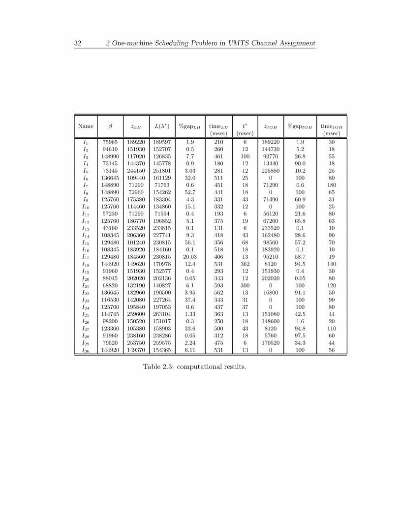
The results are reported in Table 2.3 which contains, for each instance, thefixed threshold β, the best solution zLH found by algorithm LH, the optimalsolution L2(λ∗) of the lagrangian dual problem, the percentage gap L2(λ

∗)−zLH

L2(λ∗),

the time spent by LH to solve the lagrangian dual, the time t∗ spent by LHto find the best feasible solution, the best solution zIGH found by algorithmIGH, the percentage gap L2(λ

∗)−zIGH

L2(λ∗) and the computation time for IGH.Let us begin with discussing the quality of the solutions obtained by LH

and IGH. Under this respect, LH outperforms IGH in all instances. In twothird of the instances tested (remarkably, I4, I9, I10, I12, I21, I22, I24, I28, I30),the advantage of LH is quite relevant. In seven of such instances, IGH fails infinding a feasible solution with a positive profit for user A. In eleven instances,%gapLH is smaller than 2%, and is very unsatisfactory (i.e., over 50%) in twoinstances only (I8, I15, where the performance of IGH is even worse).

Regarding the computation times we observe what follows. A time limitT1 = 150 msec imposed by voice (the most popular and time stringent ap-plication) was considered. A weaker time limit, often considered satisfactoryin multi-application settings, is T2 = 10% of the planning horizon, i.e., 0.336seconds.

The computation of the optimal value of the lagrangian dual by LH exceedsT1 in all instances but one (I13), can be carried out within T2 in eleven cases,and in the worst case (I21) takes 593 msec. Nevertheless, looking at the t∗

column, one observes that the best feasible solution found by LH is alwayscomputed largely within T1, except two cases: I18 and I21.

The behaviour of IGH is more robust. In fact, IGH finds a feasible solutionto β-FCFS within T1 in all instances but one (I7). Nevertheless, in twenty fivecases (83.3% of the instances) IGH takes more time than that required by LH

2.3. COMPUTATIONAL EXPERIENCE 31

Name #PDUs packet type #blocks #PDUs packet type #blocksA A A B B B

I1 148 m 97 130 m 74I2 130 m 74 148 m 97I3 196 m 75 273 m 169I4 196 m 75 196 m 75I5 170 ftp 150 196 m 75I6 273 m 169 170 ftp 170I7 437 m 310 273 m 169I8 262 v 131 273 m 169I9 145 m 129 262 v 131I10 117 v 60 262 v 131I11 437 m 310 117 v 60I12 170 ftp 150 262 v 131I13 257 m 102 117 v 43I14 257 m 159 145 m 129I15 273 m 121 273 m 121I16 262 v 89 145 m 129I17 145 m 129 273 m 121I18 148 m 97 170 ftp 150I19 130 m 74 262 v 89I20 148 m 105 130 m 99I21 196 m 75 437 m 289I22 170 ftp 105 170 ftp 170I23 262 v 131 170 ftp 105I24 257 v 129 262 v 131I25 170 ftp 126 170 ftp 100I26 196 m 75 273 m 86I27 148 m 97 257 v 129I28 257 v 124 262 v 89I29 170 ftp 170 162 m 84I30 145 m 129 170 ftp 150

Table 2.2: instance characteristics.

to find its best feasible solution.This well behaviour of LH is motivated by: (i) the multiplier adjustment

guided by the lagrangian relaxation rapidly converges to values yielding (throughthe algorithm of Section 2.2.2) better feasible solutions than the correspondingmechanism used by IGH; (ii) Theorem 2.2.2 allows to speed up the solutionof the lagrangian relaxation via a dichotomic search.

Based on this discussion, LH looks promising for application in real timesytems, though its implementation would require an additional effort concer-ning the development of suitable protocols and hardware supports.


Name β zLH L(λ∗) %gapLH timeLH t∗ zIGH %gapIGH timeIGH

(msec) (msec) (msec)

I1 75965 189220 189597 1.9 210 6 189220 1.9 30I2 94610 151930 152707 0.5 260 12 144730 5.2 18I3 148990 117020 126835 7.7 461 100 92770 26.8 55I4 73145 144370 145778 0.9 180 12 13440 90.0 18I5 73145 244150 251801 3.03 281 12 225880 10.2 25I6 136645 109440 161129 32.0 511 25 0 100 80I7 148890 71290 71763 0.6 451 18 71290 0.6 180I8 148890 72960 154262 52.7 441 18 0 100 65I9 125760 175380 183304 4.3 331 43 71490 60.9 31I10 125760 114460 134860 15.1 332 12 0 100 25I11 57230 71290 71594 0.4 193 6 56120 21.6 80I12 125760 186770 196852 5.1 375 19 67260 65.8 63I13 43160 233520 233815 0.1 131 6 233520 0.1 10I14 108345 206360 227741 9.3 418 43 162480 28.6 90I15 129480 101240 230815 56.1 356 68 98560 57.2 70I16 108345 183920 184160 0.1 518 18 183920 0.1 10I17 129480 184560 230815 20.03 406 13 95210 58.7 19I18 144920 149620 170978 12.4 531 362 8120 94.5 140I19 91960 151930 152577 0.4 293 12 151930 0.4 30I20 88045 202020 202136 0.05 343 12 202020 0.05 80I21 68820 132190 140827 6.1 593 300 0 100 120I22 136645 182960 190500 3.95 562 13 16800 91.1 50I23 116530 142080 227264 37.4 343 31 0 100 90I24 125760 195840 197053 0.6 437 37 0 100 80I25 114745 259600 263104 1.33 363 13 151080 42.5 44I26 98200 150520 151017 0.3 250 18 148600 1.6 20I27 123360 105380 158903 33.6 500 43 8120 94.8 110I28 91960 238160 238286 0.05 312 18 5760 97.5 60I29 79520 253750 259575 2.24 475 6 170520 34.3 44I30 144920 149370 154365 6.11 531 13 0 100 56

Table 2.3: computational results.

Chapter 3

Polyhedral study ofone-machine schedulingproblem: the case of a singleuser

3.1 Introduction

In integer programming, a typical approach in order to study a general problemconsists in finding a linear inequality description of the set of feasible points.Given a discrete optimization problem, min{cx : x ∈ S} where S ⊆ Zn

+, letus define P = {x ∈ IRn

+ : Ax ≤ b}, where A ∈ IRm×n and b ∈ IRm. We saythat P is a formulation of the original problem if and only if P ∩ Zn

+ = S. Ingeneral, it is possible to have infinite formulations associated with the sameproblem and could be very important to determine the best among them.One possible criterio to establish if formulation P1 is better than P2 consistsin solving the linear relaxation of the original problem whose solution is abound for the optimum (in particular, if we minimize the objective functionthe solution is a lower bound). Solving the linear relaxation, we calculate thevalue LB(P ); on the other hand, we can implement some heuristic to finda feasible solution x of the integer problem. The gap (x − LB(P )) certifiesthe quality of the solution. Obviously, the gap depends on the formulation;since a small gap implies a good solution, we are interested in formulationsassociated with a large lower bound. Then, if the lower bound associated withP1 is greater than the lower bound associated with P2, we conclude that P1 isbetter than P2. However, we can immediately see that this criterio dependson the objective function which is not known a priori.In alternative way, we say that P1 is better than P2 if and only if P1 ⊆ P2. The

33

34 3 Polyhedral Study: the case of a single user

set of all points that are convex combinations of points in S, i.e. the convexhull of S, conv(S), corresponds to the only formulation contained in all theother possible formulations of the original problem. Then, the objective of thepolyhedral study consists in completely describing the convex hull associatedwith the current problem: it makes to solve the linear programming problemmin{cx : x ∈ conv(S)} which is computationally easy.The total description of conv(S) can be very hard to achieve and involvesalso the study of the dimension of the convex hull. We remember that ageneral polyhedron P ⊆ IRn is of dimension d, dim(P ) = d, if the maximumnumber of affinely independent points in P is d + 1; if dim(P ) = n, then P isfull-dimensional.

To completely describe conv(S) means that we have to establish whichamong the inequalities in Ax ≤ b are indeed necessary and which not forformulating the problem.Given a general polyhedron P , we say that inequality ax ≤ a0 is valid for Pif it is satisfied by all the points in P . Given the valid inequality ax ≤ a0,the set F = {x ∈ P : ax = a0} is a face of P and we say that this inequalityrepresents F . If F 6= ∅ and F 6= P , then F is a proper face of P ; further, whenF 6= ∅ we say that inequality ax ≤ a0 supports P .We can count out of the description of conv(S) all the inequalities that arenot a support of it.In general, for a proper face F of P it happens that dim(F ) < dim(P ); ifdim(F )=dim(P )-1, then F is a maximal face or facet-defining inequality ofP . In correspondence with any facet, some inequalities exist which representP and one among them is necessary in the description of P . Instead, everyinequality representing a face F such that dim(F ) < dim(P )-1 can be removedfrom the description of P .Then, the main task of the polyhedral study consists in deciding which amongthe valid inequalities of S ⊆ Zn

+ are facets of conv(S). If we assume thatconv(S) is full-dimensional, we have two different approaches to prove thisresult depending on whether we use the definition or not. In the first case,we have to find n points in S verifying the current inequality and prove thatthey are affinely independent. Otherwise, we can suppose that there exist anhyperplane πTx = π0 containing S and select k ≥ n points in S; since thesepoints belong also to the hyperplane, we solve the associated systems. If theonly solution implies that the hyperplane coincides with the current inequality,then the result is proved. In this thesis, we will use the latter approach in orderto prove that a valid inequality is a facet.

It is possible that some inequalities are valid for lower dimensional restric-tions of S but not for S. Then, we can apply a particular procedure, calledlifting, for deriving new inequalities which are valid for S. Further, if they are

3.1. INTRODUCTION 35

also facets for some restrictions by the lifting we can try to change them infacets for S. However, observe that it is not always the case that inequalitiesvalid for restrictions are valid also for the original polyhedron.Lifting with general integer variables is computationally harder than liftingwith 0-1 variables, since in the first case the lifting procedure involves theresolution of a nonlinear integer problem. Then, from now on we assume thatS ⊆ {0, 1}n.We can illustrate the lifting principle as follows:

1. Let Sk = S ∩ {x ∈ {0, 1}n : x1 = k} for k ∈ {0, 1}. Suppose that∑ni=2 aixi ≤ α0 is valid for S0.

2. If S1 = ∅, then x1 ≤ 0 is a valid inequality for S.

3. If S1 6= ∅, then α1x1 +∑n

i=2 aixi ≤ α0 is valid for any α1 ≤ α0−γ whereγ = max{

∑ni=2 aixi : x ∈ S1}.

4. If∑n

i=2 aixi ≤ α0 is a facet of conv(S0) and α1 = α0 − γ, then α1x1 +∑ni=2 aixi ≤ α0 is a facet of conv(S).

The parameter α1 is called lifting coefficient.In general, we can start from a valid inequality for the set S∩{x ∈ {0, 1}n :

xk = 0, for some k ∈ {1, . . . , n}} and add variables xk by different sequenceseach of them may provide distinct facets. We refer to this procedure as sequen-tial lifting. Alternately, we can consider another procedure called simultaneouslifting: in this case, the coefficients of all variables that are to be lifted aresimultaneously considered, yielding inequalities that cannot be obtained bysequencial lifting. For more details on the lifting principle, see [14].Once all the facets have been calculated, we can use a lot of techniques to showthat they completely describe conv(S). Here we present seven approaches al-lowing to prove that the polyhedron P = {x ∈ {0 − 1}n : Ax ≤ b} describesconv(S).

1. Show that the matrix A, or the pair (A,b) have special structure gua-ranteeing that P =conv(S).

2. Show that points x ∈ P with fractional components are not extremepoints of conv(S) (we remember that x is an extreme point of a generalpolyhedron P if there do not exist x1 and x2 in P , x1 6= x2 such thatx = λx1 + (1 − λ)x2, λ ∈ (0, 1)).

3. Show that for all c ∈ IRn, the linear program zLP = max{cx : Ax ≤ b}has an optimal solution x∗ ∈ S.


4. Show that for all c ∈ IRn, there exists a point x∗ ∈ S and a feasiblesolution u∗ of the dual problem wLP = min{ub : uA = c, u ≥ 0} withcx∗ = u∗b. Note that this implies that the condition of the approach 3is satisfied.

5. Show that if ax ≤ a0 defines a facet of conv(S), then it must be identicalto one of the inequalities defining P .

6. Show that for any c ∈ IRn, c 6= 0, the set of optimal solutions M(c) tothe problem max{cx : x ∈ S} lies in {x : aix = bi} for some i = 1, . . . , m,where aix ≤ bi for i = 1, . . . , m are the inequalities defining P .

7. A set of linear inequalities Ax ≤ b is called Total Dual Integral (TDI)if, for all c ∈ Zn for which the linear program max{cx : Ax ≤ b} has afinite optimal value, the dual linear program min{yb : yA = c, y ≥ 0}has an optimal solution with y integral. If Ax ≤ b is TDI, b is an integervector, and P has vertices, then all vertices of P are integer.Exploiting the above definition and result, verify that Ax ≤ b is TDI.

In this work, we prove the argument by using the second approach in theabove list.

In this second part of the thesis, we will provide a polyhedral study of themax-sum competitive scheduling problem 2.1.3 illustrated in §2.1.1. Differentversions of this problem are considered, depending on the total number n ofusers in the system and on whether a feasible schedule must or may not becomplete.Given the sets of jobs and time-slots

Jk = {1, 2, . . . , nk}, k = 1, . . . , n and T = {1, 2, . . . , m}

we assume m ≥ n1 + . . . + nn. Moreover, i → j ⇔ i < j for any i, j ∈ Jk.Since the same index can denote jobs in different Jk , the superscript k will beused when necessary.

A time-indexed formulation is based on time-discretization. Since we con-sider the planning horizon T , we define 0-1 variables xk

jt for any job in Jk,k = 1, . . . , n, and for any slot t in T . Each variable specifies the assignmentof a job to a slot: precisely, xk

jt = 1 if and only if j ∈ Jk is assigned to t ∈ T .The time-indexed formulation for the general case of Problem 2.1.3 is

3.1. INTRODUCTION 37

maxm∑

k=1

∑

j∈Jk

∑

t≥j

fkj (t)xk

jt (3.1)

n∑

t=j

xkjt ≤ 1 j ∈ Jk, ∀k (3.2)

m∑

k=1

t∑

j=1

xkjt ≤ 1 t ∈ T (3.3)

xkjt −

t−1∑

s=j−1

xkj−1,s ≤ 0 j ∈ Jk, j 6= 1 t ≥ j, ∀k (3.4)

xkjt ≥ 0 j ∈ Jk, t ≥ j, ∀k (3.5)

xkjt integer j ∈ Jk, t ≥ j, ∀k (3.6)

where fkj (t) is the revenue obtained by scheduling, and therefore comple-

ting, j ∈ Jk at time t. Inequalities (3.4) represent the precedence relationsamong the jobs of Jk: if j is not the first job of Jk and is scheduled at timet, then j − 1 must be scheduled at least at time t − 1. Notice that a job (atime slot) does not need to be assigned to a time slot (a job): this variantof the problem is called Partial Scheduling Problem, PSPn (the index refersto the number of chains). To require that all jobs are scheduled, one has toreplace the sign ’≤’ with ’=’ in constraints (3.2): this variant is here referredto as Complete Scheduling Problem, CSPn. A variant of Complete Schedulingis finally when n > 1, m =

∑nk : such a variant is the Shuffling Problem,

SPn.In particular, we are interested in finding the description of the polytope

defined as the convex hull of all vectors fulfilling assignment and precedenceconstraints and having integer components. The polyhedron will be studiedin the following cases:

• n = 1, m ≥ n1 (P/CSP1)

• n = 2, m ≥ n1 + n2 (PSP2)

• n = 2, m > n1 + n2 (CSP2)

• n = 2, m = n1 + n2 (SP2)

A dynamic programming algorithm which finds an optimal solution can beprovided for several variants of the max-sum problem. We here report CSP1,CSP2 and SP2.


1. For CSP1, let f(j, s) denote the utility of an optimal solution assigningexactly j jobs of J1 to s ≥ j slots. Then

f(j, s) = max{f(j, s− 1); f(j − 1, s− 1) + f1j (s)} (3.7)

under the initial conditions f(0, s) = 0 for each s ∈ T and f(j, s) = −∞,for all j ∈ J1 and s < j. The computation requires O(n1m) time.

2. For CSP2, consider an optimal assigment of exactly j jobs in J1 and ofexactly k jobs in J2 to s ≥ j+k slots. The corresponding utility f(j, k, s)is inductively computed as:

f(j, k, s) = max{f(j−1, k, s−1)+f1j (s); f(j, k−1, s−1)+f2

k(s); f(j, k, s−1)}(3.8)

under the initial condition f(0, 0, s) = 0 for all s ∈ T . The computationrequires O(n1n2m) time.

3. For SP2, suppose that in an optimal assignment of s ≤ m slots, k slotsare assigned to (the first k jobs of) J2 and the remaining to J1. Thecorresponding utility f(k, s) is inductively computed as:

f(k, s) = max{f(k, s− 1) + f1s−k(s); f(k − 1, s− 1) + f2

k (s)} (3.9)

under the initial condition f(0, 0) = 0. Observe that f(k, s) is definedfor k ≤ s ≤ k + n1 and the computation requires O(m2) time. Formula(3.9) can be extended to P/CSP2 if fk

j (t) is non-negative regular (i.e.,non-increasing with t).

The remainder of this chapter is organized as follows:in section 3.2 we will study PSP1. We will give a time-indexed formulation ofthe problem, prove that the polyhedron defined as the convex hull of feasibleschedules is full-dimensional and completely describe it by showing that eachits vertex is integer. However, we will study some peculiar properties of theconflict graph associated with this problem. In section 3.3 we will study CSP1.We will illustrate an alternative technique to study the polyhedron associatedwith the convex hull based on the reformulation of the recursion procedureused to solve it. This approach can be applied since the problem is solvablein polynomial time.

3.2 PSP1

In this section, we study the polyhedron when only one user is in the system.The notation is simplified as follows: J1 = A, x1

jt = xjt, fj(t) = aj(t) for allj ∈ A and t ∈ T .

3.2. PSP1 39

The time-indexed formulation is

max∑

i∈A

∑

t≥i

ai(t)xit (3.10)

∑

t≥i

xit ≤ 1 i ∈ A (3.11)

∑

i≤t

xit ≤ 1 t ∈ T (3.12)

xit −t−1∑

s=i−1

xi−1,s ≤ 0 i ∈ A, i 6= 1, t ≥ i (3.13)

xit ≥ 0 i ∈ A, t ≥ i (3.14)xit integer i ∈ A, t ≥ i (3.15)

We observe that xit is defined only for t ≥ i.The assignment constraints (3.11) ((3.12)) state that each job (slot) can beassigned at most once, and the precedence constraints (3.13) state that prece-dence conditions must be satisfied.

Theorem 3.2.1. The precedence inequalities (3.13) can be reinforced to yieldthe following valid inequalities

t∑

s=i

xis −t−1∑

s=i−1

xi−1,s ≤ 0 (3.16)

for all i ∈ A, i 6= 1, and t ≥ i.

Proof. Lift variables according to the following sequence S1, . . . , S5:

S1 = {xjs : j = 1, . . . , i− 2, s ≥ j}S2 = {xis : s = i, . . . , t − 1}S3 = {xi−1,s : s = t, . . . , m}S4 = {xis : s = t + 1, . . . , m}S5 = {xjs : j = i + 1, . . . , n1, s ≥ j}

Set the lifting coefficients of S1, S3, S4, S5 to 0; those of S2, to 1. Observethat this procedure can be applied in the general case when n users are in thesystem, and then inequalities (3.16) express the precedence constraints in ageneral formulation.

Observation 3.2.1. Inequalities (3.11) are redundant for i 6= 1. Similarly,inequalities xii ≥ 0 are redundant for i 6= n1.


Proof. Inequalities (3.11) (for i = 1), (3.16) (for i = 2) and (3.14) imply

m∑

s=2

x2s ≤m−1∑

s=1

x1s ≤m∑

s=1

x1s ≤ 1

i.e., inequality (3.11) for i = 2, and so on. Moreover, inequality (3.16) fori = t = n1 writes

xn1−1,n1−1 ≥ xn1n1

Being the right-hand side ≥ 0 implies xn1−1,n1−1 ≥ 0, and so on.This result can be extended to the general case when n users are in the system.

Observation 3.2.2. Inequalities (3.12) are dominated.

Proof. From (3.11) written for i = 1 and non-negativity we have 1 ≥∑m

s=1 x1s ≥∑ts=1 x1s. Then by (3.16)

1 ≥t∑

s=1

x1s ≥ x1t +t∑

s=2

x2t ≥ x1t + x2t +t∑

s=3

x2t ≥ . . . ≥t∑

j=1

xjt.

From the observations and lifting, the time-indexed formulation of PSP1

rewrites

max∑

i∈A

∑

t≥i

ai(t)xit

∑

t≥1

x1t ≤ 1 i ∈ A (3.17)

t∑

s=i

xit −t−1∑

s=i−1

xi−1,s ≤ 0 i ∈ A, i 6= 1, t ≥ i

xit, xn1,n1 ≥ 0 i ∈ A, t > i (3.18)xit integer i ∈ A, t ≥ i

From now on, let S be the set of constraints (3.17), (3.16) and (3.18), andPS the convex hull of S.

Theorem 3.2.2. PS is full-dimensional.

3.2. PSP1 41

Proof. Suppose that PS = {x ∈ PS : πTx = 0}. Let us show that π = 0.Let eij denote the (i, j)-th unit vector, i.e. eij

ij = 1 and eijpq = 0 for all

(p, q) 6= (i, j) and define

x1s = e1s s ∈ T

xis =i−1∑

h=1

ehh + eis i ∈ A : i ≥ 2, s ∈ T : s ≥ i

Since the above vectors belong to S and have integer components, it followsπTxis = 0 for all i ∈ A and s ∈ T : s ≥ i. We then obtain

i−1∑

h=1

πhh + πis = 0 i ∈ A, s ≥ i

Hence, πis = 0.

In the following, we give a complete description of the inequalities definingPS .

Theorem 3.2.3. Inequalities∑

s≥1

x1s ≤ 1

xit ≥ 0 i ∈ A, t > i

xn1n1 ≥ 0

induce facets of PS .

Proof. See [18]

Theorem 3.2.4. Inequalities (3.16) induce facets of PS .

Proof. For i ∈ A, t ∈ T , let

Fit = {x ∈ PS :t∑

s=i

xis =t−1∑

s=i−1

xi−1,s}

Suppose that πTx = 0 for all x ∈ Fit. We next show that there exists somecostant α ∈ IR+ such that

πTx = (t∑

s=i

xis −t−1∑

s=i−1

xi−1,s) · α.


As in Theorem 3.2.2 take

x1s = e1s s ∈ T

xjs =j−1∑

h=1

ehh + ejs j ∈ A : j ≥ 2, s ∈ T : s ≥ j

These vectors belong to Fit, hence πTxjs = 0, and we obtain

πjs = 0 for 1 ≤ j ≤ i − 2, s ≥ j

Solving then the system πTxis = 0 for i ≤ s ≤ t, we get

πis = −πi−1,i−1 for i ≤ s ≤ t

Define then

ui−1,s =i−2∑

h=1

ehh + ei−1,s + eit

for i − 1 ≤ s ≤ t − 1, and solve πTui−1,s = 0. Hence

πi−1,s = −πit for i − 1 ≤ s ≤ t − 1

Finally, taking xjs for j > i, s ≥ j, and

vi−1,s =i−2∑

h=1

ehh + ei−1,s ∀s ∈ T : s ≥ t

wis =i−2∑

h=1

ehh + ei−1,t + eis ∀s ∈ T : s > t

and solving the associated systems, we see that the remaining components ofπ equal 0, and the thesis follows.

Theorem 3.2.5. Let Q denote the polytope defined by inequalities (3.17),(3.16) and (3.18). Then Q = PS .

Proof. Let x∗ be a fractional vertex of Q. Let us show that x∗ is not anextreme point of Q.

For all i ∈ A, lett(i) = min{t : x∗

it > 0}

From the precedence constraints, it follows that i < j implies t(i) < t(j). Infact

0 =t(i)−1∑

s=i

x∗is ≥

t(i)∑

s=i+1

x∗i+1,s ≥ . . . ≥

t(i)+(j−i−1)∑

s=j

x∗js

3.2. PSP1 43

Then, each of the previous sums equals 0 (from the non-negativity constraints)and t(j) > t(i) + (j − i − 1) ≥ t(i).

Let y be defined as

yit(i) = dx∗it(i)e yit = 0 ∀t 6= t(i)

for i ∈ A and t ∈ T , t ≥ i. It is immediately seen that y ∈ Q.Let then z be defined as

zit(i) =x∗

it(i)

1 − λ− λ

1 − λzit =

x∗it

1 − λ∀t 6= t(i)

for i ∈ A, t ∈ T , t ≥ i and for 0 < λ < 1, λ = min{x∗it : x∗

it > 0}. Let us showthat also z ∈ Q.

i) Trivially, z verifies inequalities (3.18).

ii) z verifies inequality 3.17. In fact, since x∗ ∈ Q, one has

m∑

s=1

z1s = z1t(1)+∑

s6=t(1)

z1s =x∗

1t(1)

1 − λ− λ

1 − λ+

∑s6=t(1) x∗

1s

1 − λ=

∑s≥1 x∗

1s

1 − λ− λ

1 − λ≤ 1

iii) z verifies (3.16). In fact

t−1∑

s=i−1

zi−1,s =

∑t−1s=i−1 x∗

i−1,s−λ

1−λ if t(i − 1) ≤ t − 1 (a)∑t−1s=i−1 x∗

i−1,s

1−λ = 0 if t(i − 1) > t − 1 (b)

and similarly

t∑

s=i

zis =

{ ∑ts=i x∗

is−λ1−λ if t(i) ≤ t (c)∑t

s=i x∗is

1−λ = 0 if t(i) > t (d)

Using these last inequalities, (a)−(d), and the fact that if t(i−1) ≤ t−1then

∑t−1s=i−1 x∗

i−1,s ≥∑t

s=i x∗is, one concludes that z satisfies (3.13).

Finally, we have x∗ = λy + (1− λ)z, which completes the proof.

We conclude this section by observing that polyhedral properties of as-signment problems can also be derived from the definition of conflict graph.The conflict graph G = (V, E) associated with an istance of PSP1 is con-structed as follows:

• each vertex of V is in a one-to-one correspondence with the variablesxjt, for j ∈ A, t ≥ j;


• two vertices in V are adjacent if and only if the corresponding variablesare incompatible, namely, cannot be set both to 1 in a feasible solu-tion. The incompatibility between variables xis and xjt can be checkedthrough the bipartite graph B = (A ∪ T, E), where jt ∈ E correspondsto xjt, and the vertices in A and T are sorted according to the job prece-dence relation and to time. Then, xis and xjt are incompatible if andonly if

(a) either the corresponding edges in A are adjacent,

(b) or cross each other,

(c) or there are more job-vertices between i and j than slot-verticesbetween s and t.

Theorem 3.2.6. Let G denote the conflict graph of PSP1. Then G is perfect.

Proof. Draw B in IR2 by associating the vertices of A and T with n1 andm equidistant points of two parallel axes r1, r2, and connecting with straightsegments the points corresponding to adjacent vertices of B. Construct thena new bipartite graph B = (A ∪ T , E) as follows. Prolong each segment jt

beyond t until all the convergent segments intersect, and draw a third axis r3

parallel to r1 and crossing all the prolonged segments. Then, E (T ) is the setof all the (points of r3 belonging to some) prolonged segment. An example ofconstruction is drawn in Figure 3.1.

Clearly, two edges in E cross each other if and only if are obtained ex-tending two edges of E for which one of (a), (b), (c) holds. Hence the conflictgraph G is the segment-intersection graph of B, which is weakly triangulatedand therefore perfect [11].Observe that the theorem can be extended to PSPn, i.e. to the case in whichn users are in the system.

Now, every feasible solution to PSP1 corresponds to a stable set of G.The converse, however, is not true: the stable set S = {22, 33, . . . , n1n1}corresponds to x22 = x33 = . . . = xn1n1 = 1, which is not feasible because doesnot schedule job 1 and therefore does not fulfill the precedence constraint. Infact, feasible solutions of PSP1 correspond to maximal stable sets of G. Hence,Theorem 3.2.6 allows us to transform PSP1 in a maximum weighted stable setproblem on G for which there exists a formulation with integer optimum,provided that the utilities ait are ≥ 0 for all i ∈ A and t ∈ T .

3.2. PSP1 45

Figure 3.1: Constructing graph B from B


3.3 CSP1

A time-indexed formulation for CSP1 is obtained from (3.10)-(3.15) by definingvariables xit for i ∈ A and t ∈ T , t ≤ i+m−n1 , and replacing the sign ’=’ for’≤’ in (3.11). For this reason, the convex hull of the feasible solutions of CSP1

is not full-dimensional. To describe it we must therefore resort to a differenttechnique from that used for PSP1.This technique is based on a reformulation of the recursion (3.7) in terms oflinear programming. The main steps of this method are as follows:

1. Consider the recursion formula which solves the integer linear problem.

2. By associating a variable to each value in the recursion, formulate alinear program .

3. Consider the dual of the linear program formulated in Step 2. This newproblem corresponds to a reformulation of the original problem and itsvariables can be reinterpreted as the original 0-1 variables.

4. From the dynamic procedure, an optimal solution of the dual problemcorresponds to an optimal sequence of decisions in the recursion. Then,the linear program has an optimal integer solution.

For more details about this technique, see [19].

Associate a variable yjt with each value f(j, t) in formula (3.7), and definethe following linear program

min yn1m (3.19)yjt − yj,t−1 ≥ 0 ∀j ∈ A, ∀t > j

y1t ≥ a1t ∀t ≥ 1yjt − yj−1,t−1 ≥ ajt ∀j ∈ A − {1}, ∀t ≥ j

An optimal solution y∗ to (3.19) is such that y∗jt = f(j, t) for j ∈ A, t ∈ T, t ≥j. Let uj,t−1, w1t and wjt be the dual variables associated with the constraintsof program (3.19). The dual reads

3.3. CSP1 47

maxn1∑

j=1

∑

t≥j

ajtwjt (3.20)

wjj − ujj − wj+1,j+1 = 0 ∀j ∈ A − {n1}wn1n1 − un1n1 = 0

uj,t−1 + wjt − ujt − wj+1,t+1 = 0 ∀j ∈ A − {n1},j < t < j + m − n1

un1 ,t−1 + wn1t − un1t = 0 n1 < t < m

uj,j+m−n1−1 + wj,j+m−n1 = 0 ∀j ∈ A − {n1}un1 ,m−1 + wn1m = 1

ujt ≥ 0 ∀j ∈ A, ∀t > j

wjt ≥ 0 ∀j ∈ A, ∀t ≥ j

Programs (3.19) and (3.20) have totally unimodular constraint matrices,so the extreme points of the latter polyhedron have all integer components.Moreover, solving (3.20) corresponds to finding an optimal solution to (3.10)-(3.15). To prove this, we show that the polyhedron associated with CSP1

can be obtained by projecting the polyhedron defined by the constraints ofprogram (3.20) into the subspace defined by u = 0. The projection procedureis described hereafter.

Projection 1

1. Rewrite the first dual constraint as

wjj − ujj − wj+1,j+1 = 0

for 1 ≤ j < n1.

2. For 1 ≤ j < n1 and j < s < j + m − n1 − 1, rewrite the third dualconstraint as

uj,s−1 + wjs − ujs − wj+1,s+1 = 0

and sum up for s = j + 1, . . . , t. Adding then the first dual constraintone gets:

s+1∑

h=j+1

xj+1,h −s∑

h=j

xjh ≤ 0

i.e., inequalities (3.16).


Projection 2

1. Rewriting the third dual constraints for j ∈ A

uj,s−1 + wjs − ujs − wj+1,s+1 = 0

and summing them up for s ∈ T, s ≥ j, we obtain

j+m−n1∑

h=j

wjh =j+m−n1+1∑

h=j+1

wj+1,h

2. Rewriting the fourth dual constraints

un1 ,s−1 + wn1s − un1s = 0

summing them up for s ≥ n1 and adding the result to the sixth dualconstraint

un1 ,m−1 + wn1m = 1

one getsm∑

h=n1

wn1h = 1

Putting together the last equation and the one obtained at step 1, weend up with

j+m−n1∑

h=j

wjh = 1 (3.21)

Given that (3.10) is equal to the objective function of(3.20) when x = w, wehave proved the following result.

Theorem 3.3.1. Inequalities (3.16) and (3.21) plus non-negativity constraintsxjt ≥ 0 (j ∈ A, j 6= n1, j < t < j + m − n1) and xn1t ≥ 0 (t ≥ n1) completelydescribe the polyhedron of CSP1.

Proof. Constraints of (3.20) constitute a complete description of its integerhull and its projection on the subspace defined by u = 0 corresponds to theappropriate constraints. See above.

Chapter 4

Polyhedral study ofone-machine schedulingproblem: the case of twousers

In this chapter we will suppose that n = 2 and separately cover the study ofPSP2, SP2 and CSP2. In 4.1, we will give a time-indexed formulation for PSP2,prove that the polyhedron defined as the convex hull of its feasible solutionsis full-dimensional, classify several valid inequalities with integral coefficientsand show that they are facets of this polytope. In 4.2 we will study SP2 anduse the technique of dynamic programming reformulation in order to describeseveral facets-inducing inequalities of the corresponding polyhedron. Finally,in 4.3 we will extend the facets obtained for SP2 to the convex hull of feasiblesolutions of problem CSP2.

4.1 PSP2

In this section, we study the polyhedron when two users are in the system.The notation is as follows:

• J1 = A, x1it = xit, f1

i (t) = ai(t) for all i ∈ A and t ∈ T

• J2 = B, x2jt = yjt, f2

j (t) = bj(t) for all j ∈ B and t ∈ T

Recalling Theorem (3.2.1) and Observation (3.2.1), the time-indexed for-mulation for PSP2 is

49

50 4 Polyhedral Study: the case of two users

max∑

i∈A

∑

t≥i

ai(t)xit +∑

j∈B

∑

t≥j

bj(t)yjt (4.1)

∑

t≥1

x1t ≤ 1 (4.2)

∑

t≥1

y1t ≤ 1 (4.3)

min{n1,t}∑

i=1

xit +min{n2,t}∑

j=1

yjt ≤ 1 ∀t ∈ T (4.4)

t∑

s=i

xis −t−1∑

s=i−1

xi−1,s ≤ 0 ∀i ∈ A, i 6= 1, t ≥ i (4.5)

t∑

s=j

yjs −t−1∑

s=j−1

yj−1,s ≤ 0 ∀j ∈ B, j 6= 1, t ≥ j (4.6)

xit, xn1n1 ≥ 0 ∀i ∈ A, t > i (4.7)yjt, yn2n2 ≥ 0 ∀j ∈ B, t > j (4.8)

xit integer ∀i ∈ A, t ≥ i (4.9)yjt integer ∀j ∈ B, t ≥ j (4.10)

Let S be the polyhedron defined by inequalities (4.2)-(4.8) and PS the convexhull of all vectors in S having integer components xit, yjt.

Theorem 4.1.1. PS is full-dimensional.

Proof. Suppose that PS = {z ∈ PS : πTz = 0}. Let us show that π = 0.Let z = (x,y) and denote as πA

it the first ((m + 1)n1 − n1(n1+1)2 ) components

of π (corresponding to A), and as πBjt the remaining ((m + 1)n2 − n2(n2+1)

2 )components (corresponding to B). For unit vectors, use the same notation asin Theorem 3.2.4.

For all i ∈ A, i ≥ 2, define

z1tA = (e1t, 0) ∀t ∈ T

zitA = (

i−1∑

h=1

ehh + eit, 0) ∀t ∈ T, t ≥ i

Since the above vectors belong to S and their components are integer, thenπTzit

A = 0 for i ∈ A and t ∈ T , t ≥ i, and it follows

i−1∑

h=1

πAhh + πA

it = 0

4.1. PSP2 51

Hence, πAit = 0, for all i ∈ A and t ≥ i.

In a similar way, for all j ∈ B, j ≥ 2, define

z1tB = (0, e1t) ∀t ∈ T

zjtB = (0,

j−1∑

h=1

ej−1,j−1 + ejt) ∀t ∈ T, t ≥ j

From πTzjtB = 0, for all j ∈ B and t ≥ j it follows

j−1∑

h=1

πBhh + πB

jt = 0

Hence, πBjt = 0 and the theorem is proved.

Observe that the result of Theorem 4.1.1 holds for PSPn.

Theorem 4.1.2. Inequalities

∑

s≥1

x1s ≤ 1

∑

s≥1

y1s ≤ 1

xit, xn1n1 ≥ 0 ∀i ∈ A, ∀t > i

yjt, yn2n2 ≥ 0 ∀j ∈ B, ∀t > j

induce facets of PS .

Proof. See [18].

Theorem 4.1.3. Inequalities (4.5) and (4.6) induce facets of PS .

Proof. Similar to Theorem 3.2.4. In fact, one can separately repeat the pro-cedure illustrated in the theorem for both users.

None of the facet-defining inequalities found so far involves variables associatedwith both A and B. The first family of inequalities with nonzero coefficientsin both sets of variables is given by the following theorem.

Theorem 4.1.4. Inequalities (4.4) induce facets of PS .


Proof. For all t ∈ T , let

Ft = {z = (x,y) ∈ PS :min{n1,t}∑

i=1

xit +min{n2,t}∑

j=1

yjt = 1}

and let πTz = π0 be any hyperplane containing Ft. We next show that

πT z = π0(min{n1 ,t}∑

i=1

xit +min{n2,t}∑

j=1

yjt)

Definez1t

A = (e1t, 0) z1tB = (0, e1t)

Since these vectors belong to Ft and have integer components, we solve πTz1tA =

π0 and πTz1tB = π0 and, for all t ∈ T obtain

πA1t = πB

1t = π0

For all i = 1, . . . , min{n1, t}, s ≥ i, s 6= t and j = 1, . . . , min{n2, t}, k ≥ j,k 6= t, define

zisA = (

i−1∑

h=1

ehh + eis, 0) + (0, e1t)

zjkB = (e1t, 0) + (0,

j−1∑

h=1

ehh + ejk)

again, plugging zisA , zjk

B into πTz = π0 and solving, one gets

πAis = πB

jk = 0

For all i = 2, . . . , min{n1, t} and j = 2, . . . , min{n2, t}, take now zitA and

zjtB as in Theorem 4.1.1. Then

πAit = πB

jt = π0

Finally, if min{n1, t} = t (min{n2, t} = t), then solve πTzisA = π0 (πTzjs

B =π0) for all i > t (j > t) and s ≥ i (s ≥ j). Hence

πAis = 0 (πB

js = 0)

4.1. PSP2 53

Now, we derive next facet-inducing inequalities of PS . The following ine-qualities have the expression

x(S1) + y(S2) ≤ 1 (4.11)

where Sk ⊆ Jk × T . That is, in a feasible schedule at most one variable ofS1 ∪S2 can be set to 1. Subsets Sk are chosen in such a way that if inequality(4.11) is violated by a solution, then so are the precedence constraints.


t∑

s=i

xis +t∑

s=t−i+1

yt−i+1,s ≤ 1 (4.12)

for i ∈ A, i ≥ 2 and t ∈ T , t ≥ i, and

t∑

s=j

yjs +t∑

s=t−j+1

xt−j+1,s ≤ 1 (4.13)

for j ∈ B, j ≥ 2 and t ∈ T , t ≥ j, induce facets of PS.

Proof. For i ∈ A, i ≥ 2 and t ∈ T , t ≥ i, let

Fit = {z = (x,y) ∈ PS :t∑

s=i

xis +t∑

s=t−i+1

yt−i+1,s = 1}

and let πT z = π0 be any hyperplane containing Fit. We next show that

πT z = π0[t∑

s=i

xis +t∑

s=t−i+1

yt−i+1,s]

For i ≤ s ≤ t and t − i + 1 ≤ h ≤ t, take the vectors zisA and zt−i+1,h

B as inTheorem (4.1.1). Since they belong to Fit and their components are integer,we solve πTzis

A = π0 and πTzt−i+1,hB = π0 and obtain

πAis = π0 −

i−1∑

h=1

πAhh i ≤ s ≤ t

πBt−i+1,h = π0 −

i−1∑

h=1

πBhh t − i + 1 ≤ h ≤ t

For 2 ≤ s ≤ t + 1 − i, define

z1sA = (

i−1∑

h=0

e1+h,s+h, 0)


and again, for 2 ≤ k ≤ i − 1 and k < s ≤ t + k − i

zksA = (

k−1∑

h=1

ehh +i−k∑

h=0

ek+h,s+h , 0)

Since k +1 ≤ s ≤ t+k− i, then i+1 ≤ s+ i−k ≤ t and all the above vectorsbelong to Fit. Solving the associated systems, for 1 ≤ k ≤ i − 1 it follows

πAkk = πA

k,k+1 = . . . = πk,t+k−1

In similar way, for 2 ≤ s ≤ i define

z1sB = (0,

t−i∑

h=0

e1+h,s+h)

and, for 2 ≤ j ≤ t − i and j < s ≤ i + j − 1

zjsB = (0,

j−1∑

h=1

ehh +t−i−j+1∑

h=0

ej+h,s+h)

Solving the systems, for 1 ≤ j ≤ t − i it follows

πBjj = πB

j,j+1 = . . . = πBj,t+j−1

For 1 ≤ k ≤ i− 1 and 1 ≤ j ≤ t − i, define

zkkA = (

k∑

h=1

ekk, 0) + (0,

t−i+1∑

h=1

eh,k+h)

zjjB = (0,

j∑

h=1

ehh) + (i∑

h=1

eh,j+h, 0)

and, plugging zkkA , zjj

B into πTz = π0, one gets

πAkk = 0 πB

jj = 0

for k ∈ A, k ≤ i − 1, and j ∈ B, j ≤ t − i. Exploiting these values of π, onerewrites

πAks = 0 k ≤ s ≤ t − i + k

πBjs = 0 j ≤ s ≤ i + j − 1

for k ∈ A, k ≤ i − 1, and j ∈ B, j ≤ t − i.

4.1. PSP2 55

For t − i + 2 ≤ s ≤ m, define

z1sA = (0,

t−i+1∑

h=1

ehh) + (e1s, 0)

and again, for 2 ≤ k ≤ i − 1 and t + k − i + 1 ≤ s ≤ m

zksA = (0,

t−i+1∑

h=1

ehh) + (k−1∑

h=1

eh,t−i+1+h + eks, 0)

Solving πTzksA = π0, one obtains

πAks = 0

for k ∈ A, k ≤ i − 1 and t + k − i + 1 ≤ s ≤ m.In similar way, for i + 1 ≤ s ≤ m define

z1sB = (

i∑

h=1

ehh, 0) + (0, e1s)

and again, for 2 ≤ j ≤ t − i and i + j ≤ s ≤ m

zjsB = (

i∑

h=1

ehh, 0) + (0,

j−1∑

h=1

eh,i+h + ejs)

Solving the associated systems, one gets

πBjs = 0

for j ∈ B, j ≤ t − i and i + j + 1 ≤ s ≤ m.For t + 1 ≤ s ≤ m, define

zisA = (0,

t−i+1∑

h=1

ehh) + (i−1∑

h=1

eh,t−i+h+1 + eis, 0)

zt−i+1,sB = (

i∑

h=1

ehh, 0) + (0,

t−i∑

h=1

eh,i+h + et−i+1,s)

Solving the associated systems, it follows that all the components of π corre-sponding to the above vectors equal 0.

Finally, for k ∈ A, k ≥ i + 1 and s ∈ T , s ≥ k define

zksA = (

k−1∑

h=1

ehh + eks, 0)


and obtainπA

ks = 0

In similar way, for j ∈ B, j ≥ t − i + 2 and s ∈ T , s ≥ j define

zjsB = (0,

j−1∑

h=1

ehh + ejs)

and obtainπB

js = 0

From the values of πAit and πB

jt the result follows. In similar way, one obtainsinequalities (4.13).

The support graph of inequality (4.12) is depicted in Figure 4.1. Firstobserve that at most one variable corresponding to a “left” (“right”) edgecan take value 1 because the corresponding job cannot be assigned more thanonce. Now, if two variables, say xis and yt−i+1,s

′ (yjs and xt−j+1,s′ ), i.e.

corresponding to one left and one right edge, take value 1, the number of timeslots before max{s, s′} is not large enough to schedule all the jobs precedingjobs i (j) of user A (B) and job t − i + 1 (t − j + 1) of user B (A).This interpretation holds for all the inequalities that we are going to present.


xit +t∑

s=i+1

xi+1,s + yt−i,t +t∑

s=t−i+1

yt−i+1,s ≤ 1 (4.14)

for i ∈ A and t ∈ T , t ≥ i + 2, and

yjt +t∑

s=j+1

yj+1,s + xt−j,t +t∑

s=t−j+1

xt−j+1,s ≤ 1 (4.15)

for j ∈ B and t ∈ T , t ≥ j + 2, induce facets of PS .

Proof. For i ∈ A and t ∈ T , t ≥ i + 2, let

Fit = {z = (x,y) ∈ PS : xit +t∑

s=i+1


s=t−i+1

yt−i+1,s = 1}


πTz = π0[xit +t∑

s=i+1


s=t−i+1

yt−i+1,s]

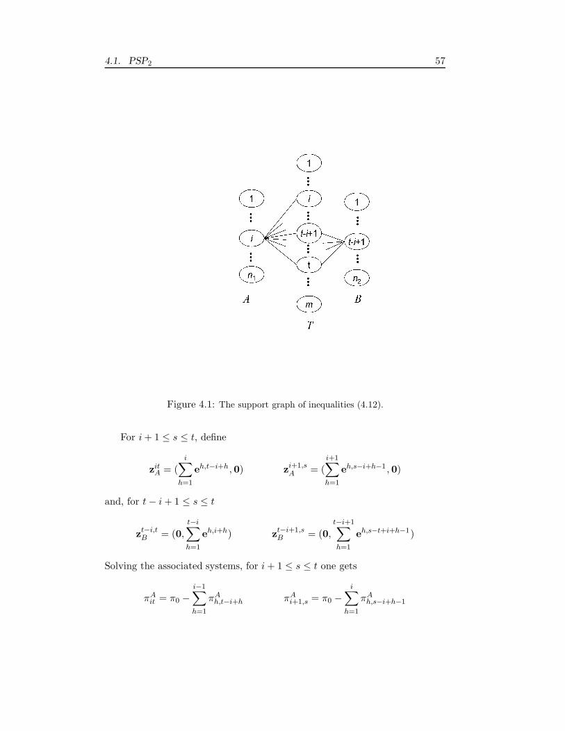
4.1. PSP2 57

Figure 4.1: The support graph of inequalities (4.12).

For i + 1 ≤ s ≤ t, define

zitA = (

i∑

h=1

eh,t−i+h , 0) zi+1,sA = (

i+1∑

h=1

eh,s−i+h−1 , 0)

and, for t − i + 1 ≤ s ≤ t

zt−i,tB = (0,

t−i∑

h=1

eh,i+h) zt−i+1,sB = (0,

t−i+1∑

h=1

eh,s−t+i+h−1)

Solving the associated systems, for i + 1 ≤ s ≤ t one gets

πAit = π0 −

i−1∑

h=1

πAh,t−i+h πA

i+1,s = π0 −i∑

h=1

πAh,s−i+h−1


and, for t − i + 1 ≤ s ≤ t

πBt−i,t = π0 −

t−i−1∑

h=1

πBh,i+h πB

t−i+1,s = π0 −t−i∑

h=1

πBh,s−t+i+h−1

For s ∈ T and k ∈ A, k ≥ i + 3, define

zi+1,sA = zit

A + (ei+1,s, 0) s ≥ t + 1

zi+2,sA = zi+1,i+1

A + (ei+2,s, 0) s ≥ i + 2

zksA = zi+1,i+1

A + (k−1∑

h=i+2

ehh + eks, 0) s ≥ k

and, for k ∈ B, k ≥ t − i + 3,

zt−i+1,sB = zt−i,t

B + (0, et−i+1,s) s ≥ t + 1

zt−i+2,sB = zt−i+1,t−i+1

B + (0, et−i+2,s) s ≥ t − i + 2

zksB = zt−i+1,t−i+1

B + (0,k−1∑

h=t−i+2

ehh + eks) s ≥ k

Solving the associated systems, it follows that all the components in π corre-sponding to the above vectors equal 0.

For s ∈ T and k ∈ A, 2 ≤ k ≤ i − 1, define

z1sA = (e1s, 0) + zt−i,t

B s ≤ i

zksA = (

k−1∑

h=1

ehh + eks, 0) + zt−i,tB k ≤ s ≤ i

ziiA = (

i∑

h=1

ehh, 0) + zt−i,tB

and again, for k ∈ B, 2 ≤ k ≤ t − i − 1

z1sB = (0, e1s) + zit

A s ≤ t − i

zksB = (0,

k−1∑

h=1

ehh + eks) + zitA k ≤ s ≤ t − i

zt−i,t−iB = (0,

t−i∑

h=1

ehh) + zitA

Solving the associated system, it follows that all the components in π corre-sponding to the above vectors equal 0.

4.1. PSP2 59

For s ∈ T , define again

zisA = (

i+1∑

h=1

eh,s−i+h , 0) i + 1 ≤ s ≤ t − 1

zisA = (

i−1∑

h=1

ehh + eis, 0) + zt−i,tB s ≥ t + 1

zt−i,sB = (0,

t−i+1∑

h=1

eh,s−t+i+h) t − i + 1 ≤ s ≤ t − 1

zt−i,sB = zit

A + (0,t−i−1∑

h=1

ehh + et−i,s) s ≥ t + 1

Also in this case, all the components in π corresponding to the above vectorsequal 0.

For s ∈ T and k ∈ A, 2 ≤ k ≤ i − 1 define

z1sA = (e1s, 0) + (0,

i∑

h=1

ehh +t−2i+1∑

h=1

ei+h,s+h)

i + 1 ≤ s ≤ 2i− 1

zksA = (

k−1∑

h=1

eh,i−k+h+1 + eks, 0) + (0,i−k+1∑

h=1

ehh +t−2i+k+1∑

h=2

ei−k+h,s+h−1)

i + 1 ≤ s ≤ 2i− k

and again, for k ∈ B, 2 ≤ k ≤ t − i − 1

z1sB = (0, e1s) + (

t−i∑

h=1

ehh +2i−t+1∑

h=1

et−i+h,s+h , 0)

t − i + 1 ≤ s ≤ 2t − 2i− 1

zksB = (0,

k−1∑

h=1

eh,t−i−k+h+1 + eks) + (t−i−k+1∑

h=1

ehh +2i−t+k+1∑

h=2

et−i−k+h,s+h−1 , 0)

t − i + 1 ≤ s ≤ 2t − 2i− k

Solving the associated system, it follows that all the components in π corre-sponding to the above vectors equal 0.

For s ∈ T and k ∈ A, 2 ≤ k ≤ i − 1 define

z1sA = e1s +

s−1∑

h=1

fhh +t−i+1∑

h=s

fh,h+1


2i ≤ s ≤ t − i + 1

zksA =

k−1∑

h=1

eh,s−k+h + eks +s−k∑

h=1

fhh +t−i+1∑

h=s−k+1

fh,h+k

2i − k + 1 ≤ s ≤ t − i + k

and again, for 2 ≤ k ≤ i − 1

z1sA = e1s + zt−i+1,t−i+1

B

s ≥ t − i + 2

zksA =

k−1∑

h=1

eh,t−i+h+1 + eks + zt−i+1,t−i+1B

s ≥ t − i + k + 1

In symilar way, for k ∈ B, 2 ≤ k ≤ t − i − 1 define

z1sB = f1s +

s−1∑

h=1

ehh +i+1∑

h=s

eh,h+1

2t − 2i ≤ s ≤ i + 1

zksB =

k−1∑

h=1

fh,s−k+h + fks +s−k∑

h=1

ehh +i+1∑

s−k+1

eh,h+k

2t − 2i− k + 1 ≤ s ≤ i + k

and again, for 2 ≤ k ≤ t − i − 1

z1sB = f1s + zi+1,i+1

A

s ≥ i + 2

zksB =

k−1∑

h=1

fh,i+h+1 + fks + zi+1,i+1A

s ≥ i + k + 1

Solving the associated system, one gets that all the components in π corre-sponding to the above vectors equal 0.

From the components of π just computed, one writes

πAit = πA

k+1,s = π0 πBt−k,t = πB

t−k+1,h = π0

for s, h ∈ T , i + 1 ≤ s ≤ t and t − i + 1 ≤ h ≤ t, and the theorem is proved.For inequalities (4.15), the proof is analougous.

4.1. PSP2 61

Figure 4.2: The support graph of inequalities (4.14).

Here again at most one x-variable (y-variable) appearing in (4.14) or (4.15)can take value 1. Further if one x-variable and one y-variable take value 1, thenthere are not enough time slots to schedule the previous jobs. The supportgraph of inequality (4.14) is depicted in Figure 4.2.


min{n1 ,t}∑

j=i

xjt +t−i∑

j=1

yjt +t∑

s=t−i+1

yt−i+1,s ≤ 1 (4.16)

for i ∈ A, i ≥ 2 and t ∈ T , 1 ≤ t − i ≤ n2 − 1, and

min{n2 ,t}∑

i=j

yit +t−j∑

i=1

xit +t∑

s=t−j+1

xt−j+1,s ≤ 1 (4.17)

for j ∈ B, j ≥ 2 and t ∈ T , 1 ≤ t − j ≤ n1 − 1, induce facets of PS.


Proof. For i ∈ A, i ≥ 2 and t ∈ T , t > i, let

Fit = {z = (x,y) ∈ PS :t∑

j=i

xjt +t−i∑

j=1

yjt +t∑

s=t−i+1

yt−i+1,s = 1}


πTz = π0[t∑

j=i

xjt +t−i∑

j=1

yjt +t∑

s=t−i+1

yt−i+1,s]

Suppose that min{n1, t} = n1 (if it is not, the procedure is analogous).Define the vector

z1tB = (0, e1t)

belonging to Fit and having integer components. Solving the system πTz1tB =

π0, one obtainsπB

1t = π0

For k ∈ A and s ∈ T , s ≥ k and s 6= t, define

zksA = (

k−1∑

h=1

ehh + eks, 0) + (0, e1t)

and solve πTzksA = π0. It follows

πAks = 0

For k ∈ A, i ≤ k ≤ min{n1, t} = n1, define

zktA = (

k−1∑

h=1

ehh + ekt, 0)

and solve πTzktA = π0. It follows

πAkt = π0

For j ∈ B, j ≤ t − i and s ∈ T , j + 1 ≤ s ≤ t − 1, define

zjjB = (

t−j∑

h=1

eh,j+h, ) + (0,

j∑

h=1

ehh)

zjsB = (

s−j∑

h=1

ehh +t−s∑

h=1

es−j+h,s+h , 0) + (0,

j∑

h=1

eh,s−j+h)

4.1. PSP2 63

Solving πTzjsB = π0, it follows

πBjs = 0 j ≤ s ≤ t − 1

For j ∈ B, 2 ≤ j ≤ t − i + 1, define

zjtB = (0,

j−1∑

h=1

ehh + ejt)

and, for s ∈ T , t − i + 1 ≤ s ≤ t − 1

zt−i+1,sB = (0,

t−i∑

h=1

ehh + et−i+1,s)

Plugging zjtB , zt−i+1,s

B into πTz = π0, one gets

πBjt = π0 πB

t−i+1,s = π0

For k ∈ A, 1 < k ≤ i − 1, define

z1tA = (e1t, 0) + (0,

t−i+1∑

h=1

ehh)

zktA = (

k∑

h=1

eh,t−k+h , 0) + (0,

t−i+1∑

h=1

ehh)

Solving πTzktA = π0, it follows

πAkt = 0 k ≤ i − 1, k 6= 1

For j ∈ B, 1 < j ≤ t − i + 1 and s ∈ T , s ≥ t + 1, define

z1sB = (

t∑

h=1

ehh, 0) + (0, e1s)

zjsB = (0,

j−1∑

h=1

eh,t−j+h+1 + ejs)

Solving πTzjsB = π0, it follows

πBjs = 0

Finally, for j ∈ B, j ≥ t − i + 2 and s ∈ T , s ≥ j, defining

zjsB = (0,

j−1∑

h=1

ehh + ejs)


and solving πTzjsB = π0, one obtains

πBjs = 0

and the theorem is proved. For inequalities (4.17), the proof is analougous.

The interpretation to these inequalities is similar to that of the previousones.

A further family of facets contains inequalities of the form

−xit + x(S1) + y(S2) ≤ 1 or − yjt + x(S1) + y(S2) ≤ 1 (4.18)

for suitable values of t ∈ T and any i ∈ A, j ∈ B. The meaning of inequalities(4.18) is the same as (4.11), but now the number of 1’s in S1 ∪ S2 depends onxit or yjt.


−yjt +t−1∑

h=t−j

xt−j,h + xt−j,s + ys−t+j,s +s∑

h=s−t+j+1

ys−t+j+1,h ≤ 1 (4.19)

for j ∈ B, j 6= n2, s, t ∈ T , t ≥ j + 2 and s > t, and

−xit +t−1∑

h=t−i

yt−i,h + yt−i,s + xs−t+i,s +s∑

h=s−t+i+1

xs−t+i+1,h ≤ 1 (4.20)

for i ∈ A, i 6= n1, t ∈ T , t ≥ i + 2 and s > t, induce facets of PS .

Proof. For more semplicity, the theorem is proved for j = 1. For any j ∈ B,the proof is analogous.

For s, t ∈ T , t ≥ 3 and s > t, let

F s1t = {z = (x,y) ∈ PS : −y1t+xt−1,t−1+xt−1,s+ys−t+1,s+

s∑

h=s−t+2

ys−t+2,h = 1}

and let πTz = π0 be any hyperplane containing F s1t. We next show that

πT z = π0(−y1t + xt−1,t−1 + xt−1,s + ys−t+1,s +s∑

h=s−t+2

ys−t+2,h).

In the rest of the proof, assume that s < 2t − 3 (if it is not, the theorem canbe proved in a symilar way).

4.1. PSP2 65

Defining

z1tB = (

t−1∑

h=1

ehh, 0) + (0,

s−t+1∑

h=1

eh,t+h−1)

and solving πTz1tB = π0, one obtains

πB1t = π0 −

t−1∑

h=1

πAhh −

s−t+1∑

h=2

πBh,t+h−1

For j ∈ B, j ≥ 2, and k ∈ T define

z1kB = (

t−1∑

h=1

ehh, 0) + (0, e1k) k ≥ t + 1

zjkB = (

t−1∑

h=1

ehh, 0) + (0,

j∑

h=1

eh,k−j+h) k ≥ t + j

Solving the associated systems, it follows

πB1k = π0 −

t−1∑

h=1

πAhh k ≥ t + 1 (4.21)

πBjk = 0 k ≥ t + j

For k ∈ T , s − t + 2 ≤ k ≤ s, defining

zs−t+1,sB = (0,

s−t∑

h=1

ehh + es−t+1,s)

zs−t+2,kB = (0,

s−t+1∑

h=1

ehh + es−t+2,k)

and solving the associated systems, one gets

πBs−t+1,s = π0 −

s−t∑

j=1

πBjj πB

s−t+2,k = π0 −s−t+1∑

h=1

πBhh

For j ∈ B, j ≥ s − t + 3 and k ∈ T , j ≤ k ≤ t + j − 1 define

zs−t+2,s+1B = (0,

s−t∑

h=1

ehh + es−t+1,s + es−t+2,s+1)

zjkB = (0,

j−1∑

h=1

ehh + ejk)


and solve the associated systems. It follows

πBs−t+2,s+1 = πB

jk = 0

For j ∈ B, 2 ≤ j ≤ s − t + 1, and k ∈ T , j ≤ k ≤ s − t + 1 define

z1kB = (

t−1∑

h=1

eh,s−t+h+1 , 0) + (0, e1k) k ≤ s − t + 1

zjkB = (

t−1∑

h=1

eh,s−t+h+1 , 0) + (0,

j−1∑

h=1

ehh + ejk)

Plugging the above vectors into πTz = π0, it follows

πB1k = π0 −

t−1∑

h=1

πAh,s−t+h+1 k ≥ 1 (4.22)

πBjk = 0

Exploting the components of π just obtained and substituting them in theexpression of πB

s−t+1,s and πBs−t+1,h, for s − t + 2 ≤ h ≤ s, one gets

πBs−t+1,s = πB

s−t+2,h = π0 − πB11 (4.23)

For j ∈ B, j ≤ s − t + 1, and k ∈ T , define

zjkB = (

k−j∑

h=1

ehh +t−1∑

h=k−j+1

eh,s−t+h+1, 0) + (0,

j∑

h=1

eh,k−j+h)

s − t + j + 1 ≤ k ≤ t + j − 2

zjkB = (0,

j−1∑

h=1

ehh + ejk +s−t+2∑

h=j+1

eh,t+h−2)

j 6= 1, s − t + 2 ≤ k ≤ s − t + j

and again, for 2 ≤ j ≤ s − t

zj,t+j−1B = (

t−2∑

h=1

eh,h+1 + et−1,s, 0) + (0, e11 +j∑

h=2

eh,t+h−1)

Solving the associated systems, one obtains that the only components of π

different from 0 are

πB1k = π0 −

k−1∑

h=1

πAhh −

t−1∑

h=k

πAh,s−t+h+1 (4.24)

πB2,t+1 = π0 − πB

11 −t−2∑

h=1

πAh,h+1 + πA

t−1,s (4.25)

4.1. PSP2 67

for s− t + 2 ≤ k ≤ t− 1. Substituting them in the expression of πB1t, it follows

πB1t = π0 −

t−1∑

h=1

πAhh − πB

2,t+1 − πBs−t+1,s (4.26)

One concludes that, thus far, the components of π whose value is differentfrom 0 are represented by (4.21)-(4.26).

Now, define the vectors

zt−1,t−1A = (

t−1∑

h=1

ehh, 0)

zt−1,sA = (

t−2∑

h=1

ehh + et−1,s, 0)


πAt−1,t−1 = πA

t−1,s = π0 −t−2∑

h=1

πAhh

For j ∈ A, j ≥ t, and k ∈ T , k ≥ j, consider

zjkA = (

j−1∑

h=1

ehh + ejk, 0)

and solve the system πTzjkA = π0. One gets

πAjk = 0

For j ∈ A, 2 ≤ j ≤ t − 1, and k ∈ T , k ≥ s − t + j + 2, define

z1kA = (e1k, 0) + (0,

s−t+2∑

h=1

ehh) k ≥ s − t + 3

zjkA = (

j∑

h=1

eh,k−j+h , 0) + (0,

s−t+2∑

h=1

ehh)

Solving the associated systems and exploiting the components of π previouslyobtained, it follows

πAjk = 0 j ≤ t − 1, k ≥ s − t + j + 2


For j ∈ A, 2 ≤ j ≤ 2t − s − 3, and k ∈ T , j ≤ k ≤ s − t + j + 1, defineagain

z1kA = (e1k, 0) + (0,

s−t+2∑

h=1

eh,t+h−2) k ≤ s − t + 2

zjkA = (

j∑

h=1

eh,k−j+h , 0) + (0,s−t+2∑

h=1

eh,t+h−2)

and solve the systems obtained plugging the above vectors into πTz = π0.Exploiting also the values of the others components of π, it follows

πA1k = π0 − πB

1,t−1 − πBs−t+2,s k ≤ s − t + 2 (4.27)

πAjk = 0

Substituting the above components in the expressions of πAt−1,t−1 and πA

t−1,s,it follows


t−1,s = π0 −t−2∑

h=2t−s−2

πAhh

Finally, for j ∈ A, 2t − s − 2 ≤ j ≤ t − 2, and k ∈ T , k ≤ t − 2, define

zjkA = (

j∑

h=1

eh,k−j+h , 0) + (0,

s−t+2∑

h=1

eh,t+h−2)

z2t−s−2,t−1A = (

2t−s−3∑

h=1

ehh + e2t−s−2,t−1, 0) + (0,

s−t∑

h=1

eh,2t−s+h−2 + es−t+1,s)

and, for j ∈ A, 2t − s − 1 ≤ j ≤ t − 2

zjkA = (

t−k+j−2∑

h=1

ehh +j∑

h=t−k+j−1

eh,h+k−j , 0) +

(0,

k−j∑

h=1

eh,j−k+t+h−2 +s−t∑

h=k−j+1

eh,t+h−1 + es−t+1,s)

t − 1 ≤ k ≤ s − t + j − 1

zjkA = (

t−k+j−2∑

h=1

ehh +j∑

h=t−k+j−1

eh,h+k−j , 0) + (0,

s−t∑

h=1

eh,2t−s+h−2 + es−t+1,s)

k = s − t + j, s − t + j + 1

4.1. PSP2 69

and again, for t ≤ k ≤ s − 1

zt−1,kA = (

t−1∑

h=1

eh,k−t+h+1 , 0) + (0,

k−t+1∑

h=1

ehh +s−t+1∑

h=k−t+2

eh,t+h−1)

Solving the associated systems, taking into account of the values previouslycomputed, one gets that the only components of π different from 0 are

πA2t−s−2,t−1 = π0 − πA

11 − πB1,2t−s−1 − πB

s−t+1,s (4.28)

πAj,t−1 = π0 − πA

11 − πB1j − πB

s−t+1,s (4.29)

πAjk = π0 − πA

11 − πB1,2t−s−1 − πB

s−t+1,s (4.30)t ≤ k ≤ s − t + j + 1

πAt−1,k = π0 − πA

1,k−t+2 − πB11 − πB

s−t+1,s (4.31)t ≤ k ≤ s − 1

for j ∈ A, 2t − s − 1 ≤ j ≤ t − 2. Substituting them in the expressions ofπA

t−1,t−1 and πAt−1,s, it follows


t−1,s = π0 (4.32)

Then, equalities (4.21)-(4.32) identify all the components of π whose value isdifferent from 0. Plugging them into πTz = π0, one concludes that for k ∈ T

such that s − t + 2 ≤ k ≤ s


t−1,s = π0

πBs−t+1,s = πB

s−t+1,k = π0 k ∈ T, s− t + 2 ≤ k ≤ s

πB1t = −π0

and all the remaining components equal 0. Then, the thesis follows.For inequalities (4.20) the proof is analogous.

Again at most one y-variable (x-variable) having coefficient equal to 1can take value 1. Further, if yjt = 0 (xit = 0) but there exists t

′ ≤ t − 1such that yjt

′ = 1 (xit′ = 1) then the number of remaining time slots is not

sufficient to schedule one job of each user and having an assignment variableappearing in the constraints plus all the previous jobs. Finally, if

∑ts=1 yjs = 0

(∑t

s=1 xis = 0), then the precedence constraints imply that none of the jobsof user B (A) having an assignment variables appearing in the constraint canbe scheduled.

The last family of facets we describe has the form

x(S1) + y(S2) ≤ 2


and derives from odd holes of the conflict graph G. To construct such a graph,observe that in PSP2 an incompatibility may arise not only between variablesxis and xjt, or yis and yjt (cases (a), (b), (c) of Section 3.2), but also betweenxis and yjt, precisely when

(d) j ≤ s − i, t = s, or

(e) j ≥ t − i + 1 and s ∈ T , j ≤ s ≤ j + i− 1.

Consider then the 5-holes on G having the form

H ′ = {xit, xi,t+1, xi+1,t+2, yt−i,t, yt−i,t+2}H ′′ = {yjs, yj,s+1, yj+1,s+2, xs−j,s, xs−j,s+2}

for i ∈ A, i ≤ n1 − 2, t ∈ T , i + 1 ≤ t ≤ m − 2, j ∈ B, j ≤ n2 − 2 and s ∈ T ,j + 1 ≤ s ≤ m − 2.

Hence, inequalities

xit + xi,t+1 + xi+1,t+2 + yt−i,t + yt−i,t+2 ≤ 2yjs + yj,s+1 + yj+1,s+2 + xs−j,s + xs−j,s+2 ≤ 2

are valid for PS . Let

f ′(i, t) = xit + xi,t+1 + xi+1,t+2 + yt−i,t + yt−i,t+2

f ′′(j, s) = yjs + yj,s+1 + yj+1,s+2 + xs−j,s + xs−j,s+2

for all i ∈ A, i ≤ n1 − 2, t ∈ T , i + 1 ≤ t ≤ m − 2, j ∈ B, j ≤ n2 − 2 ands ∈ T , j + 1 ≤ s ≤ m − 2.


f ′(i, t)+t∑

s=i+1

xi+1,s+min{t+2,n1}∑

j=i+3

xj,t+2+min{n2 ,t−i+2}∑

j=t−i+1

t+1∑

s=j

yjs+min{n2 ,t−i−1}∑

j=t−n1+2

yj,t+2 ≤ 2

(4.33)for i ∈ A, i ≤ n1 − 2 and t ∈ T , i + 1 ≤ t ≤ m − 2, and

f ′′(j, s)+s∑

h=j+1

yj+1,h+min{s+2,n2}∑

h=j+3

yh,s+2+min{n1 ,s−j+2}∑

i=s−j+1

s+1∑

h=i

xih+min{n1 ,s−j−1}∑

h=s−n2+2

xh,s+2 ≤ 2

(4.34)for j ∈ B, j ≤ n2 − 2 and s ∈ T , j + 1 ≤ s ≤ m − 2, induce facets of PS .

4.1. PSP2 71

Proof. For i ∈ A, i ≤ n1 − 2 and t ∈ T , i + 1 ≤ t ≤ m − 2, let

Fit = {z = (x,y) ∈ PS : z verifies inequalities (4.33) with sign ’=’}

and let πTz = π0 be any hyperplane containing Fit. We next show that

πT z = 2π0(f ′(i, t)+t∑

s=i+1

xi+1,s+min{t+2,n1}∑

j=i+3

xj,t+2+t−i+2∑

j=t−i+1

t+1∑

s=j

yjs+t−i−1∑

j=t−n1+2

yj,t+2)

For more semplicity, choose i ∈ A and t ∈ T in such way that t + 2 = n1

(if it is not, the theorem can be proved in symilar way).Define

zitA = (

i−1∑

h=1

ehh + eit + ei+1,t+1 + ei+2,t+2, 0)

and observe that the components whose value is 1 in the above vector corre-spond to nodes in the conflict graph G identifying a chord of H ′. Solving thesystem πTzit

A = π0, it follows

πAit = π0 −

i−1∑

j=1

πAjj − πA

i+1,t+1 − πAi+2,t+2

For k ∈ B, 2 ≤ k ≤ t − i and s ∈ T , define

z1sB = zit

A + (0, e1s) i ≤ s ≤ t − 1

zksB = zit

A + (0,

k−1∑

h=1

eh,i+h−1 + eks) i + k − 1 ≤ s ≤ t − 1

and solve the associated systems. Exploiting the just obtained value of πAit ,

one getsπB

ks = 0

for k ∈ B, k ≤ t − i, and s ∈ T , i + k − 1 ≤ s ≤ t − 1.For k ∈ B, k ≥ 2, and s ∈ T define

z1sB = zit

A + (0, e1s) s ≥ t + 3

zksB = zit

A + (0,

k−1∑

h=1

eh,t+h+2 + eks) s ≥ t + k + 2

and plug the above vectors into πTz = π0. Solving the associated systems,one obtains

πBks = 0


for k ∈ B and s ∈ T , s ≥ t + k + 2.Define again

zi,t+1A = (

i∑

h=1

eh,t−i+h+1, 0) + (0,

t−i−1∑

h=1

ehh + et−i,t+2)

Solving πTzi,t+1A = π0, it follows

πAi,t+1 = π0 −

i−1∑

h=1

πAh,t−i+h+1 −

t−i−1∑

h=1

πBhh − πB

t−i,t+2

For k ∈ B, k ≥ t − i + 2, define

zt−i+1,sB = zi,t+1

A + (0, et−i+1,s) t + 3 ≤ s ≤ 2t − i + 2

zksB = zi,t+1

A + (0,k+i−t−1∑

h=1

et−i+h,t+h+2 + eks) k + i + 2 ≤ s ≤ t + k + 1

and solve the associated systems, exploiting also the value of πAi,t+1. It follows

πBks = 0

for k ∈ B, k ≥ t − i + 1, and s ∈ T , k + i + 2 ≤ s ≤ t + k + 1.For k ∈ A, k ≥ i + 2, and s ∈ T define

zi+1,sA = zi,t+1

A + (ei+1,s, 0) s ≥ t + 3

zksA = zi,t+1

A + (k−i−1∑

h=1

ei+h,t+h+2 + eks, 0) s ≥ t + k − i + 2

Solving the associated systems, one gets

πAks = 0

for k ∈ A, k ≥ i + 1 and s ∈ T , s ≥ t + k − i + 2.Defining again

zi+2,t+2A = (

i∑

h=1

ehh +t−i∑

h=1

ei+1,t+1 + ei+2,t+2, 0) + (0,t−i∑

h=1

eh,i+h)

zt−i,t+2B = (

i−1∑

h=1

eh,t−i+h−1 + eit, 0) + (0,t−i−1∑

h=1

ehh + et−i,t+2)

4.1. PSP2 73

and solving the associated systems, one obtains

πAi+2,t+2 = π0 −

i∑

h=1

πAhh − πA

i+1,t+1 −t−i∑

h=1

πBh,i+h

πBt−i,t+2 = π0 −

t−i−1∑

h=1

πBhh −

i−1∑

h=1

πAh,t−i+h−1 − πA

it

For k ∈ A, k ≥ i + 2, define

zi+1,t+1A = zt−i,t+2

B + (ei+1,t+1, 0)

zk,t+k−i+1A = zt−i,t+2

B + (ei+1,t+1 +k−i∑

h=2

ei+h,t+h+1, 0)

and solve the associated systems in order to get

πAk,t+k−i+1 = 0

for all k ∈ A, k ≥ i + 2.Defining

zi+1,t+2A = zt−i,t

B + (e(i + 1, t + 2), 0)

zt−i,tB = (

i−1∑

h=1

eh,t−i+h−1 + ei,t+1, 0) + (0,

t−i−1∑

h=1

ehh + et−i,t)

from the associated systems, one gets

πAi+1,t+2 = 0

πBt−i,t = π0 −

t−i−1∑

h=1

πBhh −

i−1∑

h=1

πAh,t−i+h−1 − πA

i,t+1

For k ∈ B, k ≥ t − i + 2 define

zt−i+1,t+2B = zt−i,t

B + (0, et−i+1,t+2)

zk,k+i+1B = zt−i,t

B + (0,

k+i−t∑

h=1

et−i+h,t+h+1)


πBk,k+i+1 = 0


Again, for s ∈ T , i + 1 ≤ s ≤ t defining

zi+1,sA = (

i∑

h=1

eh,s−i+h−1 + ei+1,s + ei+2,t+2, 0)

and solving πTzi+1,sA = π0, one obtains

πAi+1,s = π0 −

i∑

h=1

πAh,s−i+h−1 − πA

i+2,t+2

For k ∈ B, 2 ≤ k ≤ t − i − 1, and s ∈ T , s ≤ t − i − 1 define

z1sB = zi+1,i+s+1

A + (0, e1s)

zksB = zi+1,t

A + (0,k−1∑

h=1

ehh + eks)

Solving the systems πTz1sB = π0 and πTzks

B = π0, it follows

πB(k, s) = 0

for k ∈ B, k ≤ t − i − 1, and s ∈ T , s ≤ t − i − 1.For k ∈ B, 2 ≤ k ≤ t − i and s ∈ T , s = t, t + 1 define

z1sB = zi+1,i+1

A + (0, e1s)

zksB = zi+1,i+k

A + (0,k−1∑

h=1

ehh + eks)

and solve the associated systems in order to obtain

πBkd = 0

for k ∈ B, k ≤ t − i, and s ∈ T , s = t, t + 1.For s ∈ T , t − i + 3 ≤ s ≤ t, define

zt−i+1,t−i+1B = (

i∑

h=1

eh,t−i+h+1 , 0) + (0,

t−i∑

h=1

ehh + et−i+1,t−i+1)

zt−i+1,t−i+2B = (

i∑

h=1

eh,t−i+h+1 , 0) + (0,

t−i∑

h=1

ehh + et−i+1,t−i+2)

zt−i+1,sB = (

s+i−t−1∑

h=1

eh,t−i+h +i∑

h=s+i−t

eh,t−i+h+1, 0) + (0,

t−i∑

h=1

ehh + et−i+1,s)

4.1. PSP2 75

and solve the associated systems, obtaining

πBt−i+1,t−i+1 = π0 −

t−i∑

h=1

πBhh −

i∑

h=1

πAh,t−i+h+1

πBt−i+1,t−i+2 = π0 −

t−i∑

h=1

πBhh −

i∑

h=1

πAh,t−i+h+1

πBt−i+1,s = π0 −

t−i∑

h=1

πBhh −

s+i−t−1∑

h=1

πAh,t−i+h −

i∑

h=s+i−t

πAh,t−i+h+1

Now, defining

zt−i+1,t+1B = (0,

t−i+1∑

h=1

eh,i+h)

and solving πTzt−i+1,t+1B = π0, one gets

πBt−i+1,t+1 = π0 −

t−i∑

h=1

πBh,i+h

and again, for k ∈ A, 2 ≤ k ≤ i − 1, and s ∈ T , s ≤ i, define

z1sA = zt−i+1,t+1

B + (e1s, 0)

zksA = zt−i+1,t+1

B + (k−1∑

h=1

ehh + eks, 0)

ziiA = (

i∑

h=1

ehh, 0)


πAks = 0

for k ∈ A, k ≤ i − 1, and s ∈ T , s ≤ i. Using the same definition as for theabove vectors also for k ∈ A, 2 ≤ k ≤ i, and s ∈ T , s ≥ t+2, by the associatedsystems it follows

πAks = 0

For s ∈ T , t − i + 2 ≤ s ≤ t + 1, define

zt−i+2,sB = (0,

t−i+2∑

h=1

eh,s−t+i+h−2)


and solve πTzt−i+2,sB = π0 in order to have

πBt−i+2,s = π0 −

t−i+1∑

h=1

πBh,s−t+i+h−2

and again, for k ∈ A, 2 ≤ k ≤ i − 1, and s ∈ T

z1sA = zt−i+2,t−i+2

B + (e1s, 0) t − i + 3 ≤ s ≤ t + 1

zksA = zt−i+2,t−i+2

B + (k−1∑

h=1

eh,t−i+h+2 + eks, 0) t − i + k + 2 ≤ s ≤ t + 1

solving the associated systems, one gets

πAks = 0

For k ∈ B, 4 ≤ k ≤ n2 + i − t, and s ∈ T , defining

zt−i+3,sB = zt−i+2,t−i+2

B + (0, et−i+3,s) t − i + 3 ≤ s ≤ t + 3

zt−i+k,sB = zt−i+2,t−i+2

B + (0,

t−i+k−1∑

h=1

ehh + et−i+k,s) t − i + k ≤ s ≤ t + k

and solving the associated systems, it follows that all the components corre-sponding to the above vectors equal 0.

Again, for j ∈ A, i + 3 ≤ j ≤ n1, and k ∈ B, k ≤ t − i − 1, define

zj,t+2A = (

i∑

h=1

ehh +j−i∑

h=1

ei+h,t+i−j+h+2 , 0) (4.35)

zk,t+2B = (

i∑

h=1

eh,t−i+h, 0) + (0,

k−1∑

h=1

ehh + ek,t+2)

and, solving the associated systems, one gets

πAj,t+2 = π0 −

i∑

h=1

πAh,h −

j−i−1∑

h=1

πAi+h,t+i−j+h+2

πBk,t+2 = π0 −

k−1∑

h=1

πBhh −

i∑

h=1

πAh,t−i+h

In the following, group by different families Fi the vectors allowing tocompute the values of the remaining components of π.

4.1. PSP2 77

1. For k ∈ A, k ≤ i− 1, and s ∈ T , i+1 ≤ s ≤ t− i+k, family F1 contains

zisA = (

i∑

h=1

eh,s−i+h , 0) + (0,s−i∑

h=1

ehh +t−i+1∑

h=s−i+1

eh,i+h)

i + 1 ≤ s ≤ t − 1

zksA = (

k∑

h=1

eh,s−k+h , 0) + (0,

s−k∑

h=1

ehh +t−i+1∑

h=s−k+1

eh,i+h)

zk,t−i+k+1A = (

k∑

h=1

eh,t−i+h+1, 0) + (0,t−i+1∑

h=1

ehh + et−i+2,t+1)

Solving the associated systems, from all the components of π previouslycalculated, it follows

πAks = 0

2. For k ∈ A, k ≥ i + 2, and s ∈ T , k + 1 ≤ s ≤ t + 1, family F2 contains

zkkA = (

k∑

h=1

ehh, 0) + (0,t−i∑

h=1

eh,k+h)

zksA = (

k−1∑

h=1

ehh + eks, 0) + (0,

s−k∑

h=1

eh,k−1+h + es−k+1,s+1)

Solving the associated systems, one obtains

πAks = π0 − πA

i+1,i+1 − πBt−i,t+2

3. For s ∈ T , family F3 contains vectors

zt−i−1,sB = (0,

t−i−2∑

h=1

eh,h+1 + et−i−1,s + et−i,t + et−i+1,t+1)

t − i ≤ s ≤ t − 3

zt−i,sB = (0,

t−i−1∑

h=1

ehh + et−i,s + et−i+1,t + et−i+2,t+1)

t − i ≤ s ≤ t − 2

Plugging them into πTz = π0 and solving the systems, one has that allthe resulting components of π equal 0.

4. For k ∈ B, 3 ≤ k ≤ t − i, and s ∈ T , t + 3 ≤ s ≤ 2t − i − k + 1, familyF4 contains

zksB = (

i+3∑

h=1

eh,t−i+h−1 , 0) + (0,k−1∑

h=1

ehh + eks)


Solving the associated systems, one obtains that components πBks equal

0.

5. For k ∈ B, k ≤ t− i− 2, and s ∈ T , t− i ≤ s ≤ i− 1, family F5 contains

zksB = (

i−1∑

h=1

ehh + eit + ei+1,t+1 + ei+2,t+2, 0) + (0,

k∑

h=1

eh,s−k+h)

Solving the associated systems, it follows that all the components of π

corresponding to the above vectors equal 0.

6. Finally, for k ∈ A, k ≥ i + 4, and s ∈ T , t + 3 ≤ s ≤ t + k − i, family F6

contains

zksA = (

k−1∑

h=1

ehh + eks, 0)

By the associated systems, it follows that all the components of π cor-responding to the above vectors equal 0.

At this point, solving the system containing all the equalities associatedwith components of π different from 0 but (4.35), one obtains that thesecomponents equal π0

2 . Replacing them in (4.35) and in the equalities in familyF2, it follows that all the remaining components equal 0 and the theorem isproved.For inequalities (4.34) the proof is analogous.

Finding the general form of all facet-defining inequalities corresponding tomaximal cliques of the conflict graph G and those obtained by lifting odd-holes inequalities is an open problem. We observe that by Theorem 3.2.6 nosubgraph of G induced by vertices corresponding to x (the y) variables onlycontains an odd hole.

4.2 SP2

For the shuffling problem, a time-indexed formulation is obtained from (4.1)-(4.10) by replacing first and second set of inequality constraints by equalities.Note that in this case xit (yjt) is defined only for i ∈ A (j ∈ B) and t ∈ T ,i ≤ t ≤ i + n2 (j ≤ t ≤ j + n1).

As usual, denote as PS the convex hull of feasible solutions to SP2. Somefacet-inducing inequalities of PS can be found through the same techinque asin section 3.3. Associate a variable zjt with each f(j, t) in formula (3.9), andconsider the resulting linear program

4.3. CSP2 79

min zn2m (4.36)z0j − z0,j−1 ≥ ajj j ∈ B

zjt − zj,t−1 ≥ at−j,t j ∈ B, t > j

zjt − zj−1,t−1 ≥ bjt j ∈ B, t ≥ j

Let wt−j,t and vjt be the dual variables associated with program (4.36). Thedual is

max∑

j∈J2

∑

t≥j

(at−j,twt−j,t + bjtvjt) (4.37)

wjj − v1,j+1 − wj+1,j+1 = 0 j ∈ B

vjt + wt−j,t − vj+1,t+1 − wt−j+1,t+1 = 0 j ∈ B − {n2}, t ≥ j

vn2t + wt−n2,t − wt−n2+1,t+1 = 0 t ≤ n − 1vn2n + wn−n2 ,n = 1

vjt, wt−j,t ≥ 0 j ∈ B, t ≥ j

Comparing the objective function of (4.1) to that of (4.37), one obtains wit =xit for all i ∈ A, and vjt = yjt for all j ∈ B. Observe that the solutions toSP2 are therefore in a one-to-one correspondence with (s, t)-paths of a directedacyclic grid G constructed as follows (see Figure 4.3)

• there exists a node (j, t) for each j ∈ B ∪ {0} and j ≤ t ≤ j + n1;

• s = (0, 0), t = (n2, m);

• the horizontal edges of the graph are of the form (j − 1, t − 1) → (j, t)and are weighted by bjt;

• the vertical edges are of the form (j, t− 1) → (j, t) and are weighted byat−j,t.

Being G acyclic, the convex hull of its (s, t)-paths is {z ∈ IRd|Ez = et, z ≥0}, where E is obtained by removing row s from the node-arc incidence matrixof G and d is equal to (m + 1)

∑2k=1 nk −

∑2k=1

nk(nk+1)2 .

4.3 CSP2

Problem CSP2 generalizes SP2 to the case in which m > n1 + n2. Observethat, in this case variable xit (yjs) is defined if and only if i ≤ t ≤ i + m − n1

(j ≤ s ≤ j + m − n2). Consider an optimal assigment of exactly i jobs in A


Figure 4.3: Directed acyclic graph (grid)

and of exactly j jobs in B to t ≥ i+j slots and denote as zjit the corresponding

utility. Writing the constraints derived by formula (3.8) one gets the linearprogram

min zn2n1m (4.38)

zjis − zj

i−1,s−1 ≥ ais i ∈ A, j ∈ B ∪ {0}, i + j ≤ s ≤ i + m − n1

zjis − zj−1

i,s−1 ≥ bjs j ∈ B, i ∈ A ∪ {0}, i + j ≤ s ≤ j + m − n2

zjis − zj

i,s−1 ≥ 0 i ∈ A, j ∈ B ∪ {0}, i + j ≤ s ≤ max{i + m − n1, j + m − n2}

Let wjis, vj

is and ujis be the dual variables associated with the constraints in

program . For i ∈ A, j ∈ B and s ≥ i + j, the dual is

4.3. CSP2 81

max(∑

i∈A

∑

s≥i

ais

s−i∑

j=0

wjis +

∑

j∈B

∑

s≥j

bjs

s−j∑

i=0

vjis) (4.39)

vjis + w

jis + u

ji,s−1 − v

j+1i,s+1 − w

ji+1,s+1 − u

jis = 0 i 6= n1 (4.40)

vjis + wj

is + uji,s−1 − vj+1

i,s+1 − wji+1,s+1 − uj

is = 0 j 6= n2 (4.41)vn2n1s + wn2

n1s + un2n1,s−1 − un2

n1s = 0 s ≤ m − 1 (4.42)vn2n1m + wn2

n1m + un2n1 ,n−1 = 1 (4.43)

wjis, v

jis, u

jis ≥ 0 (4.44)

Comparing to each other the objective functions of (4.1) to that (4.39), oneobtains

t−i∑

j=0

wjit = xit t ≤ i + m − n1 and

t−j∑

i=0

vjit = yjt j ≤ j + m − n2

for each i ∈ A and j ∈ B.Similarly to Section 4.2, a partial description of the convex hull PS of CSP2 isthen derived by projecting the polyhedron of program (4.39) into the subspace(w,v, z) = (w,v, 0).

Projection 1

1. Rewriting the first dual constraints for job n2 ∈ B

wn2is + vn2

is + un2i,s−1 − wn2

i+1,s+1 − un2is = 0

and summing them up for s ∈ [n2, m], and i ∈ [0, s− n2] one obtains

m∑

s=n2

s−n2∑

i=0

vn2is = 1

2. Rewriting the first dual constraints for each j ∈ [1, n2 − 1]

wjis + v

jis + u

ji,s−1 − w

ji+1,s+1 − v

j+1i,s+1 − uj

n1s = 0

and summing them up for s ∈ [j, j + m − n2) and i ∈ [0, s− j] one gets

j+m−n2∑

s=j

s−j∑

i=0

vjis =

j+1+m−n2∑

s=j+1

s−j−1∑

i=0

vj+1is


Putting together the last equation and the one obtained at Step 1, oneends up with

∑

s≥j

s−j∑

i=0

vjis = 1.

Simmetrically, for each i ∈ A one obtains

∑

s≥i

s−i∑

j=0

wjis = 1

From the correspondence between original and dual variables, it follows∑

s≥j

yjs = 1 ∀j ∈ B

∑

s≥i

xis = 1 ∀i ∈ A

i.e. the assignment constraints on the jobs.

Projection 2

1. Suppose that n2 > n1, rewrite the first dual constraints for slot t ∈ T ,t ≥ n2 + 1

whit + vh

it + uhi,t−1 − wh

i+1,t+1 − vh+1i,t+1 − uh

it = 0

and sum them up for i ∈ A, i ∈ [0, min{t, n1}], and h ∈ [0, t − i]. Theresulting equation is

min{t,n1}∑

i=max{1,t−m+n1}

xit +min{t,n2}∑

j=max{1,t−m+n2}

yjt +n2∑

j=0

min{t−1−j,n1}∑

i=0

uji,t−1

=min{t+1,n1}∑

i=max{1,t+1−m+n1}

xi,t+1 +min{t+1,n2}∑

j=max{1,t+1−m+n2}

yj,t+1 +n2∑

j=0

min t−j,n1∑

i=0

ujit

2. In particular, rewriting the equation of Step 1. for t = m it follows

xn1m + yn2m +n2∑

j=0

min{m−j,n1}∑

i=0

uji,n−1 = 1

4.3. CSP2 83

and one concludes

min{t,n1}∑

i=max{1,t−m+n1}

xit +min{t,n2}∑

j=max{1,t−m+n2}

yjt ≤ 1 (4.45)

for each t ∈ T , t ≥ n2 + 1, i.e. a particular case of the assignmentconstraints on the slots. Observe that, if n1 ≥ n2 one uses a similarprojection procedure for t ∈ T , t ≥ n1 + 1.

Projection 3

1. Rewriting the first dual constraints for job n2 ∈ B

wn2it + vn2

it + un2i,t−1 − wn2

i+1,t+1 − un2it = α

and summing them up for t ∈ [n2 + 1, m], and i ∈ [0, t− n2] it follows

∑

t≥n2+1

t−n2∑

i=0

vn2it = 1 − (wn1

1,n2+1 + un20n2

)

i.e. ∑

t≥n2+1

yn2t ≤ 1. (4.46)

Simmetrically, ∑

t≥n1+1

xn1t ≤ 1. (4.47)

2. For each j ∈ B, j 6= n2, rewrite the first dual constraints

wjit + v

jit + u

ji,t−1 − w

ji+1,t+1 − v

j+1i,t+1 − u

jit = α

and summing them up for t ∈ [j + h, m], for each h = 1, . . . , m− j, andi ∈ [0, t− j] it follows

∑

t≥j+h

t−j∑

i=0

vjit =

∑

t≥j+h+1

t−j−1∑

i=0

vj+1it +

n1∑

i=min{j,n1}

(wji,j+m−n2+1+uj

i,j+m−n2)−(

min{h,n1}∑

i=1

wji,j+h+

min{h−1,n1}∑

i=0

uji,j+h)

Observe that


• If j ≥ n1, then∑n1

i=min{j,n1}(wji,j+m−n2+1 + uj

i,j+m−n2) = 0 and one

concludes∑

t≥j+h

t−j∑

i=0

vjit ≤

∑

t≥j+h+1

t−j−1∑

i=0

vj+1it ;

• If j < n1, then variables wji,j+m−n2+1 and uj

i,j+m−n2are defined if

and only if j+m−n2+1 ≥ i+m−n1. Since i+m−n1 ≥ j+m−n1, itfollows that the above variables are defined if and only if n1 ≤ n2−1.Otherwise, one again gets

∑

t≥j+h

t−j∑

i=0

vjit ≤

∑

t≥j+h+1

t−j−1∑

i=0

vj+1it .

3. Suppose n1 ≤ n2 − 1. The first dual constraints for job n1 ∈ A and slotm − n2 + n1 + 1 ∈ T is

wjn1 ,m−n2+n1+1 + uj

n1,m−n2+n1= uj

n1 ,m−n2+n1+1

for each j < n2. Considering the same constraints for n1 ∈ A and s ∈ Tand summing up for s ∈ [m − n2 + n1 + 2, m], it follows

ujn1 ,m−n2+n1+1 = −

m∑

s=m−n2+n1+2

wjn1s ≤ 0.

4. Rewriting the first constraints for each slot s ∈ [j +m−n2 +1, m−n2 +n1 + 1]

wjis + u

ji,s−1 − w

ji+1,s+1 + u

ji+1,s = 0

and summing for i ∈ [min{j, n1}, n1], one gets

n1∑

i=min{j,n1}

(wjis +uj

i,s−1) =n1∑

i=min{j+1,n1}

(wji,s+1 +uj

is) ∀j ∈ B, j 6= n2

and concludes thatn1∑

i=min j,n1

(wji,j+m−n2+1 + uj

i,j+m−n2) = uj

n1 ,m−n2+n1+1 ≤ 0.

Then, for each j ∈ B, j 6= n2, it follows

∑

t≥j+h

t−j∑

i=0

vjit ≤

∑

t≥j+h+1

t−j−1∑

i=0

vj+1it

4.3. CSP2 85

i.e.∑

t≥j+h

yjt ≤∑

t≥j+h+1

yjt ∀j ∈ B, j 6= n2, ∀h = 1, . . . , m− j. (4.48)

which correspond to a particular case of the precedence constraints.

Simmetrically∑

t≥i+h

xit ≤∑

t≥i+h+1

xit ∀i ∈ A, i 6= n1, ∀h = 1, . . . , m− i. (4.49)

We conclude that

Theorem 4.3.1. Inequalities (4.45), (4.48), (4.49) and the job assignmentconstraints induce facets of PS .


Chapter 5

Conclusions

Studying single-machine scheduling problem, with or without precedence con-straints, is a fundamental topic investigated in a wide range of fields, especiallyin Operations Research. Depending on the particular scenario, the problemcan be conveniently formulated and several solution algorithms can be deve-loped.

In this work, we have examined two different versions of a competitivesingle-machine scheduling problem (multi-criteria, single decision-maker) withlike-chain precedence constraints and provided both a computational comple-xity investigation and a polyhedral study.In the first version, we have emphasized the competitive aspects of the model.We have considered a two-user competitive scheduling problem concerningthe allocation of two disjoint sets of unit jobs to one machine so that eitherthe worst utility is optimized (M-FCFS Problem) or the utility of one useris maximized while a minimum satisfaction level is guaranteed to the other(β-FCFS Problem). We have proved that, for separable and regular objectivefunctions of the jobs completion times the problems are NP-hard. However,we have proposed a lagrangian heuristic able to cope with a several real-timerequirements. The lagrangian dual associated with the relaxation has beensolved by a simple binary search. Further, in the case in which the solutionobtained by the heuristic is not-feasible for the original problems, we havedeveloped a very fast crossover-algorithm to adjust the current solution. Thepeculiar structure of data and feasible schedules allowed to obtain a very goodperformance of the algorithm, compared to a greedy-like heuristic on a set ofpractical instances.The main contribution of this combinatorial study consists in proposing a fastlagrangian algorithm able to compute good solutions for competitive schedu-ling problems with real-time requirements since, in general, a lagrangian re-laxation is not a suitable tool to solve problems with time restrictions.

87

88 5 Conclusions

A polyhedral study has been provided for the second version of the pro-blem, where we have optimized the sum of the total utility of each user inthe system. Unlike the previous problem, this case is solvable in polynomialtime and we have described a dynamic programming solution algorithm. Inparticular, we have distinguished between two further subproblems dependingon the fact that one or two users are in the system, and investigated somemathematical properties of them.For the case of a single user, we have completely described the polyhedrondefined as the convex hull of all feasible solutions by showing that each vertexis integer. The facets describing the polyhedron have been obtained by twodifferent techniques, depending on whether optimal schedules must or maybe complete: in the first case (CSP1 Problem), since the polyhedron of theconvex hull is not full-dimensional we have used a particular technique basedon a reformulation of the dynamic recursion formula; instead, in the secondcase (PSP1 Problem), we have proved that the polyhedron is full-dimensionaland used a well known standard technique.For the case of two users, we have computed a considerable number of facet-defining inequalities and partially described the polyhedron of the convex hull.As for one user, the polyhedron is full-dimensional when optimal schedules arepartial (PSP2 Problem), and not full-dimensional when optimal schedules arecomplete (CSP2 and SP2 Problems). Then, we have used both the techniquesjust named in order to obtain the facets.The main contribution of this polyhedral study consists in including the prece-dence constraints in the time-indexed formulation of a single-machine schedu-ling problem and having a description of the polytope defined as the convexhull of feasible solutions. In fact, before this work a similar polyhedron wasinvestigated but either precedence relations were not considered or the originalproblem was formulated in terms of completion times instead of time-indexedvariables. The fact that this description is complete when only one user isin the system is a very important result which made easier the study for twousers.

At present, further research should aim at using the facet-defining inequa-lities obtained from the polyhedral study to improve the bound provided bylinear relaxation of the minimum satisfaction constraint (β-FCFS Problem).Our idea consists in adding valid inequalities, and studying the computationalfeatures of both linear and lagrangian relaxations with the aim of devising anefficient implicit enumeration algorithm.

Bibliography

[1] A. Agnetis, P. Mirchandani, D. Pacciarelli, A. Pacifici, NondominatedSchedules for a Job-Shop with Two Competing Users, Computationaland Mathematical Organization Theory 6:2 (2000): 191 - 217

[2] A. Agnetis, P. Mirchandani, D. Pacciarelli, A. Pacifici, Scheduling Prob-lems with Two Competing Users, Dipartimento di Informatica e Au-tomazione, Universita ”Roma Tre”, RT-DIA-67-01(2001), and OperationResearch, forthcoming

[3] P.J. Brewer and C.R. Plott, A Binary Conflict Ascending Price (BICAP)Mechanism for the Decentralized Allocation of the Right to Use RailroadTracks, Intarnational Journal of Industrial Organization, 1996, 14, pp.857-886

[4] K.R. Baker and J.C. Smith, A Multiple-Criterion Model for MachineScheduling, Journal of Scheduling, 6: 7-16 (2003)

[5] M. Albani, C. Arbib, V. Arvia, G. Ciaschetti, F. Del Sorbo, L. Dimopolou,A. Giralda, S-H. Oh, G. Politis, J.M. Sanchez, D.C. Schultz, G. Sciasciaand M. Servilio, FUTURE Deliverable D03.02 – Software Implementationof the FUTURE QoS Procedures, April 2002.

[6] FUTURE project web site: http://www.ebanet.it/future.htm

[7] M.R. Garey and D.S. Johnson, Computers and Intractability: A Guideto the Theory of NP-Completeness, Freeman & Co., S. Francisco, 1979.

[8] F.W. Glover and M. Laguna, Tabu Search, McGraw-Hill, 1995.

[9] M.X. Goemans and R. Ravi, The Constrained Minimum Spanning TreeProblem, Proc. Scandinavian Workshop on Algorithmic Theory, LectureNotes in Computer Science 1097, Springer-Verlag, 1996, pp. 66-75.

[10] L.A. Hall, Approximation Algorithms for Scheduling, in D.D. Hochbaum:Approximation Algorithms for NP-Hard Problems, PWS Publishing Com-pany, Boston, MA, 1997.

89

90 BIBLIOGRAPHY

[11] G. Lancia, R. Carr, B. Walenz and S. Istrail, 101 Optimal PDB StructureAlignments: a Branch-and-Cut Algorithm for the Maximum Contact MapOverlap Problem, Proceedings of the fifth annual international conferenceon Computational biology (2001) 193-202

[12] J.Y-T. Leung and G.H. Young, Preemptive Scheduling to MinimizeWeighted Flow Time, Information Processing Letters 34 (1990) 47-50.

[13] G.Y. Lin and J.J. Solberg, Integrated shop floor control using autonomousagents, IIE Transactions, 1992, (24), 3, pp. 57-71

[14] G.L. Nemhauser and L.A. Wolsey, Integer and Combinatorial Optimiza-tion, Wiley, New York (1988)

[15] M. Queyranne and A.S. Schulz, Polyhedral Approaches to MachineScheduling, Technical Report 408/1994, Department of Mathematics,Technical University of Berlin

[16] J.P. Sousa and C. Ramos, A distributed architecture and negotiationprotocol for scheduling in manufacturing systems, Computers in Industry,1991, (38), 2, pp. 103-113

[17] J.P. Sousa and L.A. Wolsey, Time Indexed Formulations of Non-Preemptive Single-Machine Scheduling Problems, Mathematical Pro-gramming: Series A, v.54, n.3, pp.353-367, 1992

[18] J.M. van den Akker, C.P.M. van Hoesel and M.W.P. Savelsbergh, A Poly-hedral Approach to Single-Machine Scheduling Problems, MathematicalProgramming (1999) 541-572

[19] L. Wolsey, Strong Formulations for Mixed Integer Programming: A Sur-vey, Mathematical Programming 45 (1989) 173-191

[20] M.P. Wellman, W.E. Walsh, P.R. Wurman and J.K. MacKie-Mason, Auc-tion Protocols for Decentralized Scheduling, Games and Economic Behav-ior (2001), 35, pp. 271-303

Documents

One-Machine Scheduling with Unit Jobs and Chain Precedence Relations · Universita degli Studi Roma Tre` Dottorato di Ricerca in Informatica e Automazione XVII Ciclo - 2005 Mara Servilio